Persistent C II Absorption in the Normal Type Ia Supernova 2002fk

Abstract

We present well-sampled $UBVRIJHK$ photometry of SN 2002fk starting 12 days before maximum light through 122 days after peak brightness, along with a series of 15 optical spectra from -4 to +95 days since maximum. Our observations show the presence of C II lines in the early-time spectra of SN 2002fk, expanding at  11,000 km s${}^{-1}~{}$and persisting until  8 days past maximum light with a velocity of $\sim$9,000 km s${}^{-1}~{}$. SN 2002fk is characterized by a small velocity gradient of $\dot{v}_{Si~{}II}=26$ km s^-1 day^-1, possibly caused by an off-center explosion with the ignition region oriented towards the observer. The connection between viewing angle of an off-center explosion and the presence of C II in the early time spectrum suggests that the observation of C II could be also due to a viewing angle effect. Adopting the Cepheid distance to NGC 1309 we provide the first $H_{0}$ value based on near-IR measurements of a Type Ia supernova between 63.0$\pm$0.8 ($\pm$ 2.8 systematic) and 66.7$\pm$1.0 ($\pm$ 3.5 systematic) km s^-1 Mpc${}^{-1}~{}$, depending on the absolute magnitude/decline rate relationship adopted. It appears that the near-IR yields somewhat lower (6-9%) $H_{0}$ values than the optical. It is essential to further examine this issue by (1) expanding the sample of high-quality near-IR light curves of SNe in the Hubble flow, and (2) increasing the number of nearby SNe with near-IR SN light curves and precise Cepheid distances, which affords the promise to deliver a more precise determination of $H_{0}$.

1 INTRODUCTION

Type Ia supernovae (SNe) have proven to be extremely useful as extragalactic distance indicators in the optical (Hamuy et al., 2006; Hicken et al., 2009; Folatelli et al., 2010) thanks to the relation between peak luminosity and decline rate (Phillips, 1993), which allows the standardization of their luminosities, and in the near infrared (Wood-Vasey et al., 2008; Krisciunas et al., 2004b, c) where they behave almost as standard candles (Kattner et al., 2012). Photometric observations of SNe Ia have delivered Hubble diagrams with unrivaled low dispersions (0.15 mag), which permits one to determine precise values for fundamental cosmological parameters such as the Hubble constant and the deceleration parameter. It was this technique that led in 1998 to the surprising discovery that the Universe is in a state of accelerated expansion caused by a mysterious dark energy that comprises 70% of the energy content of the Universe (Riess et al., 1998; Perlmutter et al., 1999). Measuring the equation of state parameter of the dark energy and its evolution with time constitutes one of the most important astrophysical challenges today.

Since the discovery of the accelerated expansion, extensive surveys and follow-up programs have increased the number of SNe Ia by more than an order of magnitude. Furthermore, the quality of the follow–up observations (light curves, early–time optical spectra, near-infrared (near-IR) spectra, nebular spectroscopy, polarization) has significantly increased. As a consequence of the increase in the statistical samples available and the degree of details observed, several indications of diversity have emerged within the family of SNe Ia that manifest in differences in several observables, most notably, early time velocity gradients (Benetti et al., 2004), the presence of unburned material, late-time nebular velocity shifts (Maeda et al., 2010a, c), line polarization (Leonard et al., 2005; Wang & Wheeler, 2008), high-velocity components of spectral lines (Kasen et al., 2003; Thomas et al., 2004; Gerardy et al., 2004; Mazzali et al, 2005), and interstellar line strengths (Sternberg et al., 2011; Foley et al., 2012d; Förster et al., 2012; Phillips et al., 2013). At this point the use of SNe Ia for the determination of cosmological parameters and the equation of state of the dark energy is dominated by systematics (see e.g. Kessler et al., 2009; Conley et al., 2011). Among the most important sources of systematics are the extinction by dust in the SN host galaxies (Folatelli et al., 2010, and references therein) and our lack of understanding of the explosion mechanisms and the progenitor system (see e.g. Hillebrandt & Niemeyer, 2000; Röpke et al., 2012; Maoz et al., 2014).

SNe Ia are believed to result from the nuclear burning of a C+O white dwarf (WD). Given that carbon is not produced in the explosion, it provides unique evidence of the original composition of the star before explosion. For this reason the amount and distribution of the unburned carbon material is fundamental to understand the burning process of the star. Until recently only a handful of normal SNe Ia have shown carbon. Thanks to large surveys that have discovered and followed–up SNe Ia from very early phases, carbon has been found in nearly 30% of the SNe before maximum light (Parrent et al., 2011; Thomas et al., 2011b; Folatelli et al., 2012; Silverman & Filippenko, 2012b), and even more frequently within the class of very luminous and low expansion velocities objects thought to be the result of a super–Chandrasekhar–mass WD (Howell et al., 2006; Thomas et al., 2007; Yamanaka et al., 2009; Scalzo et al., 2010; Silverman et al., 2010).

Additional multi-wavelength and multi-epoch observations of SNe Ia will be required to establish a scenario connecting the observed diversity among SNe Ia. Here we present a contribution to this subject through extensive optical and near-IR observations for the normal Type Ia SN 2002fk obtained in the course of the “Carnegie Type II Supernova Survey” (CATS, hereafter) (Hamuy et al., 2009). While our optical data are complementary to the photometry published by the Lick Observatory Supernova Search (LOSS, Riess et al., 2009b; Ganeshalingam et al., 2010), and by the Center for Astrophysics (CfA) Supernova Program (CfA3 sample, Hicken et al., 2009), our near-IR data provide one of the earliest near-IR light curves for a Type Ia SN. The exceptional coverage of the maximum both in the optical and the near-IR light curves together with the Cepheid distance recently measured by Riess et al. (2011a, 2009a), makes SN 2002fk one of the most suitable SNe Ia for calibration of the Hubble constant. The completeness of the light curves also affords the opportunity to test independent methods for the determination of the host galaxy reddening using a mixture of B Vand V-near–IR colors. In addition, we present 15 optical spectra obtained from $-4$ to $+95$ days since maximum in the $B$-band, which are complemented by spectra obtained by the CfA Supernova Program (Blondin et al., 2012) and the Berkeley Supernova Ia Program (BSNIP, Silverman et al., 2012a). The spectra provide clear evidence for unburned carbon. SN 2002fk is a very well observed SNe Ia showing carbon lines in pre-maximum spectra and the only one where such lines persist several days past peak brightness. Thus, these observations provide important clues to our understanding of the explosion mechanisms for normal SNe Ia.

This paper is organized as follows: in section 2 we describe the photometric and spectroscopic observations and data reductions; in section 3 we present the photometric data and the determination of reddening caused by dust; in section 4 we show the spectroscopic evolution of SN 2002fk; in section 5 we calculate the Hubble constant using the photometry presented here complemented by LOSS and CfA3 photometry, and the distance to NGC 1309 (Riess et al., 2011a); we discuss our results and present our conclusions in section 6. In an upcoming paper (Zelaya et al., 2014) we will present spectropolarimetric observations of SN 2002fk.

2 OBSERVATIONS AND DATA REDUCTION

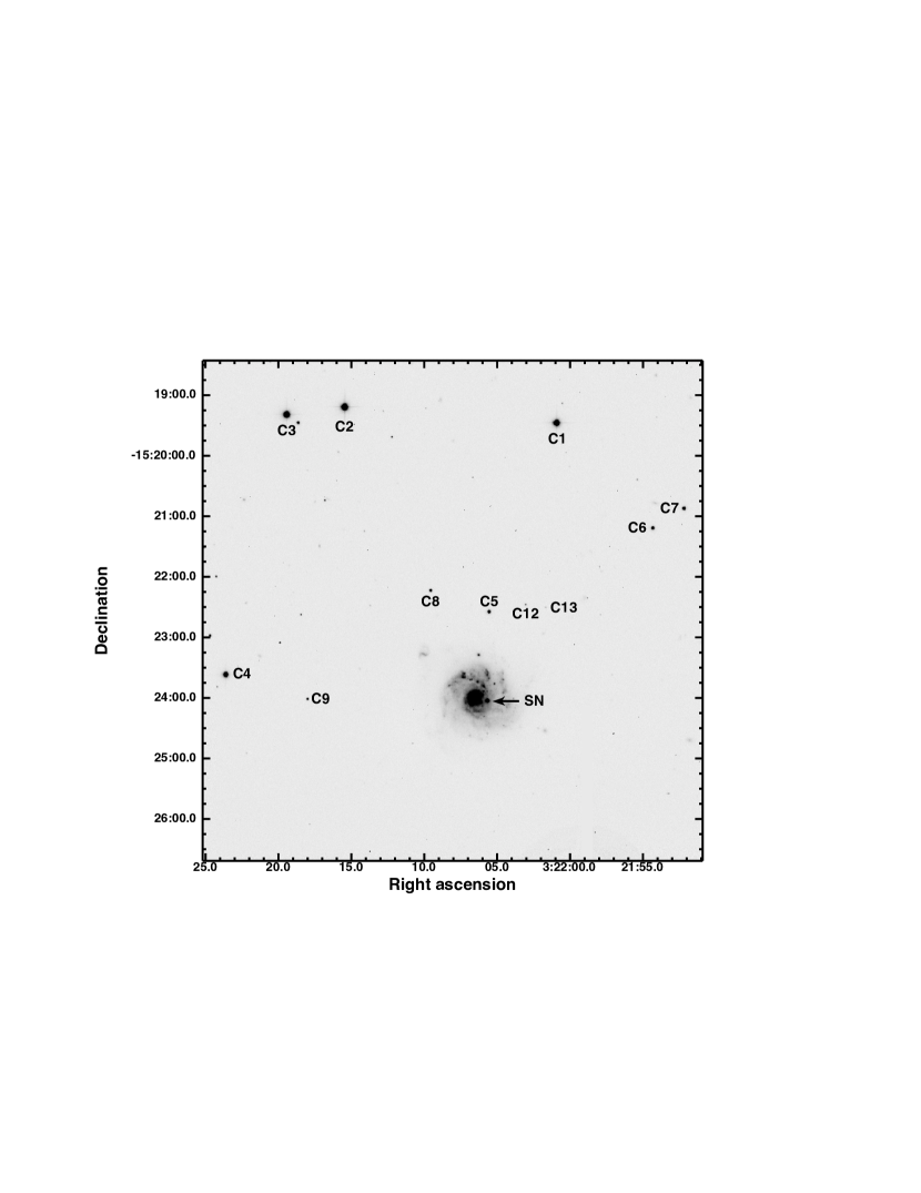
Figure 1: Field of SN 2002fk observed with the Swope telescope. North is up and east is to the left. SN 2002fk is marked with an arrow and eleven stars of the local standard stars used to derive differential photometry are labeled.

SN 2002fk was discovered independently by Kushida, R. (2002) and by Wang & Qiu (2002) at $V\simeq 15.0$ mag on 2002 September 17.7. The supernova was located at $\alpha$=03:22:05.71 and $\delta$=-15:24:03.2 (J$2000$), $3.6^{\prime\prime}$ south and $12.6^{\prime\prime}$ west of the host galaxy NGC 1309 (see Figure 1). NGC 1309 is an SA(s)bc galaxy with a heliocentric recession velocity of 2,136 km s${}^{-1}~{}$obtained from neutral hydrogen line measurements (Koribalski et al., 2004). Ayani & Yamaoka (2002) classified SN 2002fk as a Type Ia from an optical spectrum obtained on 2002 September 20.

2.1 Instrumental Settings

The optical imaging of SN 2002fk was obtained with UBVRI Johnson-Kron-Cousins filters using the Swope 1 m telescope, the Wide Field Re-imaging CCD Camera (WFCCD) on the 2.5 m du Pont telescope, and the Low-Dispersion Survey Spectrograph (LDSS-2) on the 6.5 m f/11 Magellan Clay telescope, all at Las Campanas Observatory (LCO). A few additional optical images were obtained with the 0.9 m and 1.5 m telescopes at Cerro Tololo Inter-American Observatory (CTIO). For galaxy subtraction, we used images obtained with the Direct CCD Camera on the 2.5 m du Pont telescope. Additional observations with the Panchromatic Robotic Optical Monitoring and Polarimetry Telescope (PROMPT) at CTIO were obtained for the single purpose of calibrating a photometric sequence of local standards around SN 2002fk.

IR images of SN 2002fk were obtained with $JHK_{s}$ filters with the Swope telescope IR Camera (C40IRC) and the Wide Field IR Camera (WIRC) on the du Pont telescope. In Table 1 we summarize the instruments used for the optical and IR imaging.

Optical spectroscopy of SN 2002fk was obtained with five instruments: LDSS-2 and the B&C Spectrograph on the LCO Baade telescope, the WFCCD and Modular Spectrograph on the LCO du Pont telescope, and FORS1-PMOS on the ESO (European Southern Observatory) Very Large Telescope located on Cerro Paranal. In Table 2 we summarize the instruments used for the spectroscopic follow-up and their main characteristics. More details about these instruments are given by Hamuy et al. (2009).

2.2 Optical Photometry Reduction

We reduced the optical images using a custom IRAF script package, as described by Hamuy et al. (2009). We processed the raw images through bias subtraction and flat fielding. As long as sky flats were available, we corrected small gradients in dome flat illumination ($\thicksim 1\%$). To reduce any possible galaxy contamination in our photometry we subtracted the host galaxy from our SN images using high quality template images obtained with the Direct CCD Camera on the du Pont telescope after the SN had vanished on 2005 February 13. This instrument delivers a typical point-spread-function (PSF) of $0.7^{\prime\prime}$ (full width at half-maximum intensity), thus providing templates with better image quality than any of the SN+galaxy images. To secure high quality image subtractions, we employed the same $UBV(RI)_{KC}$ filter set of the Swope telescope (which was used on the majority of our optical observations; see Table 5). Differential PSF photometry was made on the galaxy-subtracted images using the sequence of local standards (Figure 1), calibrated against Landolt (1992) photometric standards observed during several photometric nights. Systematic errors introduced by using template images taken with the du Pont telescope are considered in Appendix A.

The Landolt stars were employed to derive the following photometric transformations from instrumental to standard magnitudes,

$$U~{}=~{}u~{}+~{}ct_{u}~{}(u~{}-~{}b)~{}+~{}zp_{u}$$ (1)

$$B~{}=~{}b~{}+~{}ct_{b}~{}(b~{}-~{}v)~{}+~{}zp_{b}$$ (2)

$$V~{}=~{}v~{}+~{}ct_{v}~{}(v~{}-~{}i)~{}+~{}zp_{v}$$ (3)

$$R~{}=~{}r+~{}ct_{r}~{}(v~{}-~{}r)~{}+~{}zp_{r}$$ (4)

$$I~{}=~{}i+~{}ct_{i}~{}(v~{}-~{}i)~{}+~{}zp_{i}$$ (5)

In these equations $UBVRI$ (left-hand side) are the published magnitudes in the standard system Landolt (1992), $ubvri$ (right-hand side) correspond to the natural system magnitudes, $ct_{j}$ to the color term, and $zp_{j}$ to the zero-point for filter $j(j=u,b,v,r,i)$.

These transformations were then applied to 11 pre-selected stars in the field of the SN in order to establish a sequence of local standards, which is presented in Table 3. In Appendix B we perform a detailed analysis of our photometric calibration and a comparison with that obtained by LOSS (Ganeshalingam et al., 2010) and CfA3 (Hicken et al., 2009).

Having established the photometric calibration of the SN 2002fk field, we carried out differential photometry between the SN and the local standards. For all five optical cameras we employed average color terms determined on multiple nights (listed in Table 4), solving only for the photometric zero-points. The resulting $UBVRI$ magnitudes covering 130 days of evolution of SN 2002fk are summarized in Table 5.

2.3 Near-IR Photometry Reduction

The vast majority (21/24) of the near-IR photometric observations were obtained with WIRC on the du Pont telescope. WIRC has four different detectors. Usually only two of the detectors were used to observe. The observing strategy consisted in taking five dithered images of the object with detector 1, while detector 2 was used to take $sky$ images. Then the detectors were switched, i.e. the SN was observed on detector 2 while detector 1 was used to take $sky$ images. The observations were reduced following standard procedures with a slighty modified version of the Carnegie Supernova Project (CSP) WIRC pipeline (written in IRAF, Hamuy et al., 2006; Contreras et al., 2010). We had to modify the pipeline to work without dark and bias because these calibrations were not taken during the observations of SN 2002fk. The pipeline first masks detectable sources in the sky frames and then combines them to create a final sky frame for each detector. Then the pipeline subtracts the final sky image from the science images to get a bias/dark/sky subtracted science frame. In order to correct for pixel–to–pixel gain variations we divide science images by a flat field constructed from the subtraction of a flat-off from a flat-on image and normalize the result. For nights where flats were not taken we used the best calibration images from the two closest nights. In addition to this, the pipeline masks cosmetic defects and saturated objects and combines the dithered frames from each detector to deliver a final science image per detector.

Classic-Cam on the 6.5 m Baade telescope was used on three nights to obtain near-IR images. Since all calibrations (dark, bias, flat) were taken with this instrument, we performed the standard data reduction. First we subtracted the bias and the dark from all frames. Then we created a flat field for each night subtracting the flat–off from the flat–on image and normalized the result. Finally, we corrected pixel–to–pixel variations dividing all science images by the flat fields.

We obtained galaxy subtraction templates, using the WIRC/du Pont configuration, on 2003 November 2 and 11 after the SN had vanished. We perfomed differential PSF photometry of the SN in the WIRC galaxy–subtracted images with respect to four near-IR local sequence stars around SN 2002fk. We calibrated these four local standards stars with respect to Persson et al. (1998) standards using aperture photometry. The Persson standard star images were taken close in time and airmass to the SN field, so it was not necessary to correct for atmospheric extinction. Photometry of the local sequence was obtained in four photometric nigths with WIRC. In Table 6 we present our $JHK_{s}$ photometry for the local sequence along with the 2MASS magnitudes for comparison. Within the uncertainties our photometry is in good agreement with the 2MASS values. This is an encouraging result considering that the Persson et al. (1998) system is not identical to the 2MASS photometric system (Skrutskie et al., 2006).

In the small field-of-view of Classic-Cam only star c5 was observed along with the SN. This precluded us from subtracting the galaxy templates and performing PSF photometry, so we ended up measuring aperture photometry of the SN with respect to c5 alone. Table 7 presents the resulting $JHK_{S}$ photometry for SN 2002fk which covers 115 days of its evolution since discovery.

2.4 Spectroscopy

A total of 15 spectra of SN 2002fk were obtained, as summarized in Table 2. We obtained five spectra with the 6.5 m Magellan Baade telescope using LDSS-2. For these observations, a 300 line mm^-1 grism blazed at $5000$ Å  was employed, covering from 3600 to 9000 Å with a resolution of 14 Å. Three spectra were observed with the Baade telescope using the B&C Spectrograph. This instrument uses a SITe $1752\times 572$ pixel CCD with 300 line mm^-1 grating blazed at $5000$ Å. The wavelength range obtained was 3200 to 9200 Å with a resolution of 7 Å. Three times we used the du Pont telescope with the WFCCD instrument in its spectroscopic long-slit mode. A 400 line mm^-1 blue grism was employed, covering the wavelength range from 3800 to 9200 Å with a resolution of 8 Å. We also obtained one spectrum with the Las Campanas Modular Spectrograph on the du Pont telescope, covering from 3790 to 7270 Å with a resolution of 7 Å. With all four instruments (WFCCD, LDSS-2, B&C, and Modular Spectrograph) we observed the SN and the standard stars with the slit aligned along the parallactic angle (Filippenko, 1982) to reduce the effects of atmospheric dispersion. Additional information about the instruments and observing modes are presented in Hamuy et al. (2009).

Three of our spectra of SN 2002fk were obtained in polarimetric mode with the FORS1 instrument on the ESO VLT UT3 telescope on 2002 October 1st, 5th, and 14th. For each of the three epochs observed, four exposures were taken with the retarder plate at position angles of 0, 22.5, 45 and 67.5 degrees. The exposure times were 720 sec on October 1st, 720 sec on October 5th, and 600 sec on October 14th. Grism GRIS_300V was used with no order separation filter. This provides a dispersion of 2.59 Å pix^-1, and the resulting wavelength range 3300–8500 Å. The spectral resolution with a 1^′′ slit was 12.25 Å, which we measured using the [OI] 5577 sky emission line. Additional observations of a flux standard, EG21, were performed at position angle 0 degrees to calibrate the flux level. We followed a standard data reduction procedure using IRAF. A single intensity spectrum was obtained for each epoch, combining the four angle spectra with two beams each, in the following way:

$${F_{tot}=\frac{\sum\frac{spec_{i}}{specerr_{i}^{2}}}{\sum\frac{1}{specerr_{i}^{2}}}}$$ (6)

with i=0, 22, 45 and 67, where $spec_{i}$ is the sum of the two beams corresponding to ordinary and extraordinary rays, at each angle, and $specerr_{i}$ is the quadratic sum of the errors per beam for each of the four angles. Here we present the intensity spectra alone, and we postpone the spectropolarimetric reduction details and results for an upcoming paper (Zelaya et al., 2014).

Despite having observed the SN along the parallactic angle, we checked the spectrophotometric quality of our spectra by convolving them with the standard $BV(RI)_{KC}$ bandpasses described by Bessell (1990) and computing synthetic magnitudes. In general, this comparison shows very good agreement within $0.01$-$0.03$ mag between the observed and synthetic colors, thus demonstrating the excellent quality of our spectra. Having checked the relative spectrophotometry we proceeded to apply a low–order wavelength dependent correction to make all of our spectra fully consistent with the photometry.

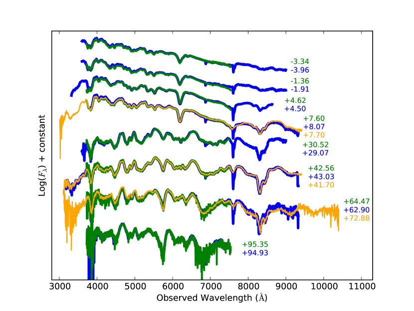
Figure 2: Comparison between our spectra (blue), the CfA (green, Blondin et al., 2012), and the BSNIP (orange, Silverman et al., 2012a) spectra taken at similar epochs. The phase is indicated on the right for each spectrum.

Optical spectra of SN 2002fk were recently published by the CfA Program (Blondin et al., 2012) and the Berkeley Supernova Ia Program (BSNIP, Silverman et al., 2012a). CfA obtained 23 spectra covering from $-3$ to $+120$ days since maximum in $B$ and BSNIP obtained five spectra from $+8$ to $+150$ days after $B$ maximum. In Figure 2 we compare our spectra (blue) taken with the CfA (green) and the BSNIP (orange) spectra observed within one day from ours. As can be seen, the agreement is excellent, with only very small differences with the first two CfA spectra. All of these data will be used subsequently in our study.

3 LIGHT CURVES OF SN 2002fk

3.1 Optical Light Curves

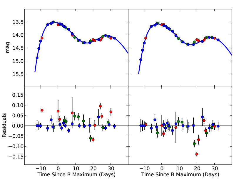
Figure 3: Upper left. $I$-band light curve of SN 2002fk (red=CATS, blue=LOSS, green=CfA3) before applying the photometric offset found in the calibration of the local standards. Bottom left. Magnitude residuals from the polynomial fit (blue line). Upper right. $I$-band light curve of SN 2002fk after applying the photometric offset caused by systematic differences in the local standards, along with a polynomial fit (blue line). Bottom left. Magnitude residuals from the polynomial fit.

Optical photometry of SN 2002fk has been previously published by LOSS (Riess et al., 2009b; Ganeshalingam et al., 2010) and by the CfA Supernova Program (CfA3 sample, Hicken et al., 2009). These data have good sampling, most notably the LOSS observations that begin $11.8$ days before $B$-band maximum. These datasets are a valuable complement to our optical photometry. However, since we have detected systematic differences between the CATS, LOSS, and CfA3 photometric calibrations it has proven necessary to apply offsets to the LOSS and CfA3 photometry in order to bring all measurements to the same CATS photometric system, as described in Appendix B. In doing so, we added in quadrature to the LOSS and CfA3 uncertainties those from the photometric offsets. Adding these offsets (summarized in Table 8) decrease significantly the differences in the $R$- and $I$–band SN magnitudes among the three datasets (as illustrated in Figure 3 for the $I$–band), but has no noticeable effects in the $B$- and $V$–bands.

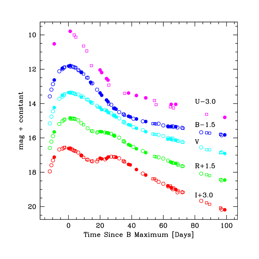
Figure 4: Optical light curves of SN 2002fk. Filled circles are our observations, open circles correspond to LOSS measurements, and open squares to CfA3 data. Photometry of LOSS and CfA3 were shifted by the offsets given in Table 8 to bring them into our CATS photometric system (as discussed in Appendix B).

Figure 4 presents the $UBVRI$ light curves of SN 2002fk, including CATS (filled circles) and the LOSS (open circles) and CfA3 data (open squares) after applying the corresponding photometric offsets. A polynomial fit to the B-band light curve around maximum brightness yields $B_{max}=13.30\pm 0.03$ mag on JD $2,452,547.8\pm 0.5$ and a decline rate parameter $\Delta m_{15}=1.02$ $\pm 0.04$ which is close to the fiducial value adopted by Phillips et al. (1999) and Folatelli et al. (2010) for SNe Ia. Polynomial fits to the other lightcurves yield $U_{max}=12.69\pm 0.07$ mag on JD $2,452,546.0\pm 1.5$, $V_{max}=13.37\pm 0.03$ mag on JD $2,452,548.5\pm 0.5$, $R_{max}=13.36\pm 0.03$ mag on JD $2,452,549.2\pm 0.5$, and $I_{max}=13.57\pm 0.03$ mag on JD $2,452,545.8\pm 0.5$. $V$ and $R$ peak roughly one day after $B$, whilst $U$ and $I$ peak two days before $B$. This is consistent with the typical behavior of SNe Ia. Bright Type Ia SNe usually show a secondary maximum in $R$ and $I$, and in the near-IR bands. A polynomial fit to the secondary peaks yields $R_{2^{nd}~{}max}=14.14\pm 0.03$ on JD $2,452,568.3\pm 0.5$ and $I_{2^{nd}~{}max}=14.08\pm 0.03$ on JD $2,452,575.4\pm 0.5$. Errors in peak magnitudes include the uncertainty due to differences in filter transmissions (S-corrections; see Appendix C).

A small bump $\sim 0.15$ mag is present in the $I$-band light curve of SN 2002fk located $\sim 20$ days past maximum and $\sim 7.5$ days before the secondary maximum. This is seen in Figure 3 which shows the individual $I$-band data points and the residuals from a polynomial fit. The left panels correspond to the original CATS, LOSS, and CfA3 data, while the right panels correspond to the same data after applying the photometric offsets. Although the bump in question is supported by three photometric points (two from CATS and one from CfA3), each one with a 3-7 $\sigma$ significance, we cannot rule out the possibility that it is an artifact due to the combination of photometry taken with different filters and detectors.

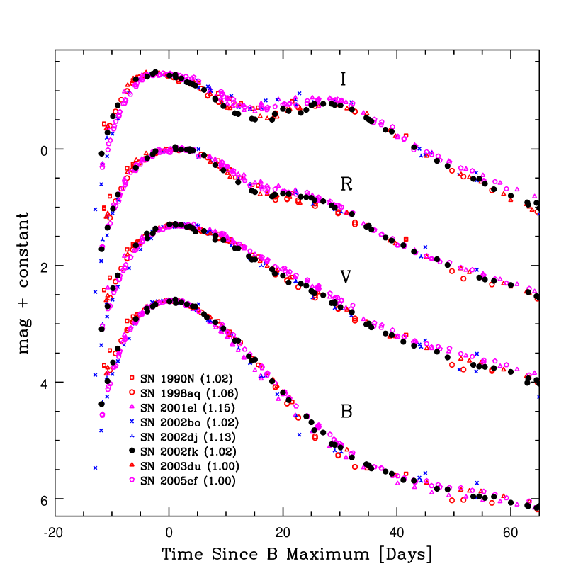
Figure 5: $BVRI$ light curves of SN 1990N, SN 1998aq, SN 2001el, SN 2002bo, SN 2002dj, SN 2002fk, SN 2003du, and SN 2005cf, (Lira et al., 1998; Riess et al., 2005; Krisciunas et al., 2003; Benetti et al., 2004; Pignata et al., 2008; Stanishev et al., 2007; Wang et al., 2009) selected for their similar decline rates, normalized to peak brightness. $\Delta m15$ is given in parenthesis for each SN.

In Figure 5 we compare the $BVRI$ light-curves of SN 2002fk and other SNe with similar $\Delta m15$. Despite their similar decline rates, we notice small yet real departures from a commom photometric behavior, namely: 1) a dispersion in the rise branch, where SN 2002bo, SN 2002dj, and SN 2005cf show faster rise times, in agreement to what was found by Pignata et al. (2008) and Ganeshalingam et al. (2011) where high-velocity gradient objects (as defined by Benetti et al., 2005) generally show shorter rise times; 2) the small bump $\sim 0.15~{}mag$ in the $I$–band light curve of SN 2002fk that peaks $20$ days past maximum in $B$; 3) small differences in the time and amplitude of the secondary peaks in $R$ and $I$ (see also Krisciunas et al., 2001; Folatelli et al., 2010; Burns et al., 2011).

3.2 Near-IR Light Curves

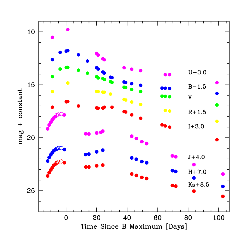
Figure 6: Our optical and Near-IR photometry of SN 2002fk. In $JHK$ bands open symbols are data obtained with Classic-Cam, whilst filled symbols correspond to WIRC observations.

Figure 6 shows our optical and near-IR light curves of SN 2002fk. Our near-IR observations begin 12 days before $B$-maximum, among the earliest $JHK$ photometry ever obtained for a SN Ia, and extend through 102 days past maximum which is exceptional for a SN Ia (Krisciunas et al., 2004b; Wood-Vasey et al., 2008; Folatelli et al., 2010). The photometric coverage is remarkably good before and close to peak brightness, through the near-IR minimum, and at late times. The second near-IR peak, on the other hand, is not so well sampled. Polynomial fits to the IR light curves around maximum brightness yield $J_{max}=13.76\pm 0.02$ on JD $2,452,544.3\pm 0.5$, $H_{max}=13.98\pm 0.02$ on JD $2,452,543.5\pm 0.5$, and $K_{max}=13.76\pm 0.02$ on JD $2,452,544.2\pm 0.5$.

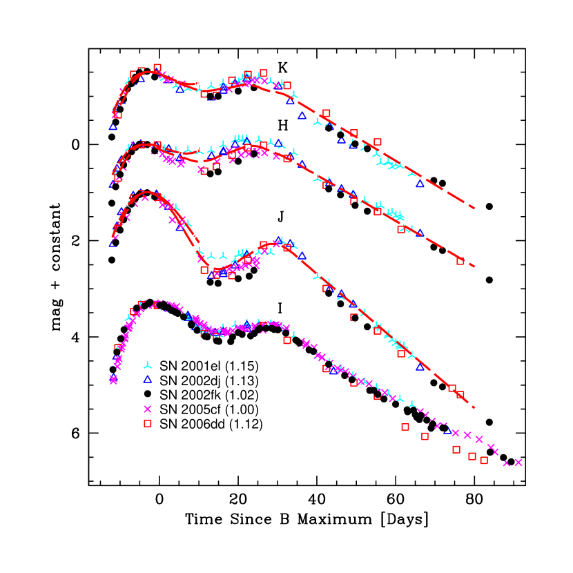
Figure 7: $IJHK$ light curves of SN 2001el (cyan), SN 2002dj (blue), SN 2002fk (black), SN 2005cf (magenta), and SN 2006dd (red), selected for their similar decline rates, normalized to peak brightness. We chose to compare the templates of Krisciunas et al. (2004b) (dotted-dashed line) and Wood-Vasey et al. (2008) (dashed line). $\Delta m15$ is given in parenthesis for each SN.

In Figure 7 we compare the $IJHK$-band light curves of SN 2002fk, SN 2001el (Krisciunas et al., 2003), SN 2002dj (Pignata et al., 2008), SN 2005cf (Wang et al., 2009), and SN 2006dd (Stritzinger et al., 2010) normalized to peak magnitudes in each band. These are well-studied SNe with very complete optical and near-IR light curves and with similar $\Delta m_{15}$ values. We also show in dotted-dashed lines the templates from Krisciunas et al. (2004b) and in dashed lines the templates from Wood-Vasey et al. (2008). In all bands SN 2002fk has a faster rise to peak than both templates. After maximum it is evident that SN 2002fk has a more pronounced minimum in all $IJHK$ bands compared with the other SNe and a deeper minimum than the Wood-Vasey et al. (2008) and Krisciunas et al. (2004b) templates. Although the secondary peak was not covered by our observations in $JHK$, the observations suggest a well defined secondary maximum, clearly distinguishable from the first peak and from the minimum between the peaks. The differences in the light curves become much smaller around the secondary peak, after which all five SNe show good agreement in their decline rates.

Kasen (2006) showed that the near–IR secondary maximum is related to the ionization evolution of the iron group elements, in particular to the transition of the iron/cobalt gas from double to singly ionized. In his scenario the mixing of ⁵⁶Ni outward increases the velocity extent of the iron core. This hastens the ocurrence of the near–IR secondary maximum. In SN 2002fk the secondary peak does not occur earlier than in the remaining SNe, so a large mixing of ⁵⁶Ni is unlikely. Higher metallicity progenitors should produce a higher fraction of stable iron group material (Timmes et al, 2003). Kasen (2006) showed that a large amount of iron group material would cause the recombination wave to reach the iron–rich layers relatively earlier, thus producing an earlier secondary maximum. Given that in SN 2002fk the secondary peak was not observed to occur earlier, greater than normal progenitor metallicity is also unlikely. In his models, Kasen (2006) presented evidence that a higher contrast between the peaks and the minima is expected in hotter SNe (i.e. those with relatively greater ⁵⁶Ni mass) because the transition wave from double to single ionized iron takes a longer time to reach the iron core. Perhaps then, the deep minimum observed in SN 2002fk is produced by a higher than normal ejecta temperature, and the $I$-band bump $\sim$20 days past maximum could be due to asymmetries in the distribution of iron group elements.

3.3 Reddening Determination

Given the early and complete optical and near-IR light curves of SN 2002fk we can estimate the amount of dust reddening (Galactic + host galaxy) using different colors, assuming the standard Galactic extinction law of Cardelli et al. (1989).

Firstly, we estimate the reddening towards SN 2002fk from its late-time $(B-V)$ colors using the standard Lira–Phillips relation (Lira, 1996; Phillips et al., 1999), which yields $E(B-V)_{Lira}=0.066\pm 0.019$. The slope of SN 2002fk is in good agreement with the Lira relation within the dispersion. Secondly, we use the near maximum optical colors versus decline rate relations (Phillips et al., 1999), which yields $E(B-V)_{B_{max}-V_{max}}=0.009\pm 0.044$ and $E(B-V)_{V_{max}-I_{max}}=0.082\pm 0.038$. Thirdly, we estimate the reddening using the $V-$ near-IR colors by minimizing $\chi^{2}$ between the observed $V-H$ and $V-K$ colors with respect to the Krisciunas et al. (2004b) zero-reddening templates. From these fits we obtain $E(B-V)_{V-H}=0.014\pm 0.037$ and $E(B-V)_{V-K}=0.075\pm 0.036$. Within the uncertainties these results are consistent with the optical methods.

In table 9 we summarize our results. The weighted mean of the reddening using these five different methods is $E(B-V)=0.057$ with a dispersion of $0.036$ mag. This value is close to the measured Galactic reddening towards SN 2002fk, namely $E(B-V)=0.035$ mag (Schlafly & Finkbeiner, 2011), which implies that the host galaxy reddening was low. As shown by Phillips et al. (2013), the equivalent width of Na I D is not a reliable indicator of host dust extinction in SNe Ia. According to these authors, only the absence of detectable Na I D absorption in a high signal-to-noise ratio spectrum can be used to infer low dust extinction. The fact that we detect a weak (0.018 Å) Na I D absorption in our highest signal-to-noise spectra at the redshift of the host galaxy is consistent with the small dust reddening inferred from the SN colors.

3.4 Optical Colors

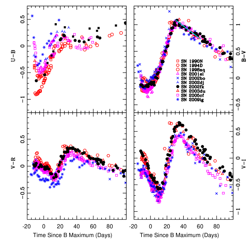
Figure 8: Optical colors of SN 2002fk (in black). For comparison, in red are shown the LVG SN 1990N, SN 1994D, SN 1998aq, and SN 2003du. In magenta are shown the LVG SN 2001el and SN 2005cf with strong HV Ca II near maximum, and in blue the HVG SN 2002bo, SN 2002dj and SN 2009ig.

Figure 8 shows dust corrected color curves of well observed “normal” SNe Ia with similar $\Delta m_{15}$ to SN 2002fk. We dereddened the color curves using the recalibrated Galactic extinction maps of Schlegel et al. (1998) presented by Schlafly & Finkbeiner (2011) and the host galaxy reddening derived from the Lira–Phillips relation (Lira, 1996; Phillips et al., 1999). In all cases we transformed reddening into extinction at different filters using the standard Galactic extinction law of Cardelli et al. (1989) with $R_{V}=3.1$, with the warning that the use of $R_{V}=3.1$ can introduce systematic offsets for heavily reddened SNe like SN 2002bo (Phillips et al., 2013), with the effect being largest in $V-I$. In red are shown SN 1990N (Lira et al., 1998), SN 1994D (Patat et al., 1996), SN 1998aq (Riess et al., 2005), SN 2003du (Stanishev et al., 2007) which are LVG SNe. In magenta we show SN 2001el (Krisciunas et al., 2003) and SN 2005cf (Wang et al., 2009) both of which are LVG with strong high velocity Ca II lines near maximum light. Finally in blue are SN 2002dj (Pignata et al., 2008), SN 2002bo (Benetti et al., 2004), and SN 2009ig (Foley et al., 2012a) which are HVG SNe.

In the upper left panel of Figure 8 we show the $U-B$ color curves. Overall, we see an evident dispersion amounting to several tenths of a magnitude, despite all SNe having been corrected for dust reddening. We see a progression in color before and near maximum, where the LVG SNe display the bluest colors, the LVG SNe with strong high-velocity (HV) Ca II lines have intermediate colors, and the HVG SNe are the reddest. What is more remarkable is the difference in shape between the two most complete $U-B$ color curves. While SN 1998aq grows steadily redder in $U-B$ during the first 30 days, SN 2005cf shows a dramatic blueing at early epochs followed by an upturn seven days before maximum. The evolution of SN 2002fk is similar to SN 1994D, evolving with a linear trend from very blue $U-B$ colors at pre-maximum epochs to redder colors at about 30 days past maximum. It is important to note at this point, that even though the dispersion in $U-B$ colors can be significantly affected by systematic errors in dust reddening corrections, the differences in shape cannot be accounted by this effect. Although filter transmission variations can reach a few tenths of a magnitude in the $U$-band, the differences observed at early epochs reach even one magnitude, so we believe they are real and not a result of filter mismatches or sky transmission.

The upper right panel of Figure 8 shows the $B-V$ colors. Overall, the color evolution of SN 2002fk is that of a normal Type Ia. The four SNe with the earliest observations (SN 1994D, SN 2002bo, SN 2005cf, SN 2003du, and SN 2009ig) all show clear evidence for un upturn around 5 days before maximum that indicates an evolution from red to blue at the very early epochs. Even though the sample is small, this seems to be a generic feature of SNe Ia. This behavior was already noted by Hamuy et al. (1991) in SN 1981D, based on early-time observations obtained with photographic plates (see their Fig. 5). Promptly after maximum all SNe grow redder for a period of $\sim$30 days, after which they all grow bluer which corresponds to the linear tail of the optical light curves. As a reference we show with solid line the Lira law (in cyan). Within the uncertainties it appears that all SNe share a common slope at these epochs, but we observe small systematic offsets of $\sim$0.08 mag for some individual objects. Considering that the use of different instrumental bandpasses can introduce systematic errors $\sim$0.05 mag at these epochs (Stritzinger et al., 2002), it appears that there are some small yet significant intrinsic color differences among SNe Ia during the phase corresponding to the Lira law.

The $V-R$ colors are shown in the lower left panel of Figure 8. The evolution of SN 2002fk has a normal shape compared to the other SNe. However, we see an intrinsic scatter at the level of 0.4 mag among the different objects, with SN 2002fk and SN 1998aq being among the reddest objects. SN 2005cf and SN 2001el, which are LVG objects with strong HV Ca II lines, are in the middle of the distribution, while the HVG objects are among the bluest objects. Note that this is the opposite trend that we observe in $U-B$. This apparent gradient in $V-R$ color is specially noticeable 10 days before B maximum. At later times this gradient still seems to be present, but there is more scatter in the photometry.

In the lower right of Figure 8 we show the $V-I$ color curves. We see evidence for a divergent behaviour at the very earliest epochs. We can separate the SNe in two groups before maximum; the SN 2002fk-like SNe (LVG SNe without strong Ca II before maximum) showing a steady evolution from red to blue; the SN 2005cf-like group (LVG SNe with strong Ca II lines); and the HVG SNe, that show a downturn at day $\sim$-7. At about ten days before maximum, the former are nearly 0.3 mag redder then the latter. An interesting case is SN 2009ig which belongs to the HVG group (Foley et al., 2012a) and is slightly redder than SN 2005cf, but at $\sim$-15 days shows redder colors than the remaining SN 2005cf-like objects. The early-time dichotomy observed in $V-I$ is reminiscent of what happens in $U-B$. Interestingly, both the $U$ and $I$ bands share the presence of Ca II lines, namely the Ca II H&K lines at 3951 Å and the Ca IR triplet at 8579 Å. However, as demostrated by Cartier et al. (2011) the strength of the Ca II lines cannot completely explain the dichotomy observed in $U-B$ and $V-I$. About 10 days past $B$ maximum all SNe grow redder through 40 days after peak. Later on, all SNe grow bluer. Although the slope is similar we observe significant offsets that exceed the potential systematic errors due to the use of different instrumental bandpasses (Stritzinger et al., 2002).

3.5 $V~{}-$ near-IR Colors

Figure 9 shows the dereddened $V~{}-$ near-IR colors of SN 2002fk. For comparison we show the $V~{}-$ near-IR color curves of SN 2001el (Krisciunas et al., 2003), SN 2002dj (Pignata et al., 2008), SN 2003du (Stanishev et al., 2007), SN 2005cf (Wang et al., 2009), and SN 2006dd (Stritzinger et al., 2010). These are well studied SNe with similar $\Delta m_{15}$, early, and complete near-IR light curves. As in Section 3.4, we corrected the colors making use of the Galactic extinction maps of Schlafly & Finkbeiner (2011), the Lira–Phillips relation to estimate host galaxy reddening, and the Cardelli et al. (1989) extinction law to transform from color excess to extinction in specific bandpasses. We caution the reader that our choice of $R_{V}=3.1$ may introduce significant offsets in the $V$–near-IR colors of heavily reddened objects with a lower value of $R_{V}$.

We show in Figure 9 the $V~{}-$ near-IR templates of Krisciunas et al. (2004b). In dotted-dashed lines are shown the loci for slow decliners while dashed lines correspond to the loci of mid-range decliners. In the top panel we show the $V-J$ colors. SN 2002fk declines from blue to red at a similar rate as the locus of slow decliners, but is offset by $\sim$0.2 mag to redder colors. At early epochs SN 2002fk is similar to SN 2002dj, SN 2003du, and SN 2006dd. After ten days since maximum SN 2002fk is similar to SN 2001el, and SN 2005cf.

The middle panel of Figure 9 shows the $V-H$ color curves. Here SN 2002fk fits the locus of the mid-range decliners at early epochs but after ten days SN 2002fk is $\sim$0.2 mag bluer than the template. At early times SN 2002fk has similar colors to SN 2002dj, SN 2003du, SN 2005cf, and SN 2006dd. SN 2002dj and SN 2006dd resemble the mid-range decliners template. After 10 days since maximum, the evolution of SN 2002fk continues to be similar to SN 2005cf.

The $V-K$ color curve is shown in the botton panel of Figure 9. SN 2002fk matches the template quite well, although at early epochs it is slighty redder than the locus of the mid-range decliners. SN 2002dj is very similar to SN 2002fk, whereas SN 2001el, SN 2003du, and SN 2005cf show colors that better fit the locus of the slow decliners.

4 OPTICAL SPECTRA

Figure 10 shows 15 optical spectra of SN 2002fk that span from four days before B maximum to 95 days past peak. Near maximum, SN 2002fk shows the characteristic Si II $\lambda 6355$ absorption, Ca II H&K lines, the Ca II near-IR triplet, the W-shaped S II lines, and Si III $\lambda 4560$. Nugent et al. (1995) found a correlation between peak luminosity and R(Si II), the ratio of the intensities of Si II $\lambda 5972$ to Si II $\lambda 6355$ lines near maximum, which is interpreted as a temperature effect. For SN 2002fk we measure R(Si II) = 0.189 $\pm$ 0.002, corresponding to a bright SN with a hot ejecta (see section 5, Nugent et al., 1995). Further evidence that SN 2002fk was hotter than normal can be drawn from the blue B Vcolors, and from the Si III $\lambda 4560$ and $\lambda 5740$ absorption lines before maximum, which are usually present in the early spectra of bright SNe.

A relatively weak yet evident absorption is present at $\sim 6400$ Å, which we identify as C II $\lambda 6580$. This line was previously identified by Blondin et al. (2012) in a spectrum taken $-3.34$ days since maximum. Support for this identification comes from two additional lines at $\sim 4600$ Å and $\sim 7000$ Å which can also be attributed to C II. Remarkably, the C II $\lambda 6580$ feature persists until several days past maximum, which is unprecedented in normal SNe Ia (see Parrent et al., 2011; Thomas et al., 2011b; Folatelli et al., 2012; Silverman & Filippenko, 2012b). Otherwise, the post-maximum evolution of SN 2002fk is consistent with that of a Branch-normal Type Ia SNe (see section 4.1 below).

4.1 Temporal Evolution of the Spectra

In Figure 11 we compare the spectra of SN 2002fk with three well-observed SNe with similar $\Delta m15$: SN 1998aq (Branch et al., 2003), SN 2003du (Stanishev et al., 2007), and SN 2005cf (Wang et al., 2009; Bufano et al., 2009), the prototypical Branch-normal SN 1994D (Patat et al., 1996), and the super–Chandra candidate SN 2006gz (Hicken et al., 2007). We choose -4, 0, +25 and +95 days after maximum light as comparison epochs. All the spectra are in the host galaxy rest-frame and were reddening corrected as described in Section 3.4.

In the top-left of Figure 11 we show the spectra of SN 2002fk at $\sim-4$ days. The spectrum is characterized by lines of singly ionized intermediate-mass elements (Si, S, Mg, and Ca), higher-ionized lines of Si III, C II, and a strong absorption at $\sim 3750$ Å  that could correspond either to high-velocity Ca II H&K, Si II $\lambda 3858$, or a blend of both (see Section 4.4). At this epoch the spectrum of SN 2002fk is similar to SN 2003du with both SNe showing strong Si III absorption lines. Also the super–Chandra candidate SN 2006gz shows prominent Si III lines. Like SN 2002fk, SN 2006gz also shows strong C II $\lambda 6580$ absorption, which is broader than the ones in SN 2002fk. If the HV Ca II lines are present in SN 2002fk, they are slightly stronger than the ones observed in SN 1994D, but not as remarkable as the HV Ca II lines present in SN 2005cf at this epoch.

In the top-right panel of Figure 11 we show the spectrum of SN 2002fk near maximum light. At this epoch SN 2002fk and SN 1998aq share similar spectral shape and features and both SNe show Si III lines comparable to the lines present in SN 2006gz. Additionally, SN 2002fk shows normal Ca II, and maybe weak HV Ca II lines. In contrast SN 2005cf shows strong HV Ca II lines. Remarkably, SN 2002fk still shows clear C II $\lambda 6580$ and $\lambda 7234$ absorption lines.

In the bottom-left of Figure 11 we show the spectrum of SN 2002fk at $\simeq+25$ days since maximum. This epoch corresponds to the beginning of the transition from the photospheric to the nebular phase and the spectra are becoming dominated by absorption of iron–peak elements (Fe II, Co II, Cr II, etc). The similarity of all the spectra at this epoch is impressive. However, it is interesting to mention that the Na I absorption in SN 2002fk is slightly stronger than in the others. In the bottom-right of Figure 11 we show the spectrum of SN 2002fk and other SNe at $\simeq+95$ days since maximum. At this epoch the transition from photospheric to nebular phase is almost complete, and all the spectra are very similar showing forbidden emission lines of iron elements (i.e. [Fe III], [Co III]). SN 2002fk is particularly similar to SN 1998aq, and still has a slightly stronger Na I absorption line.

4.2 Photospheric Expansion Velocity

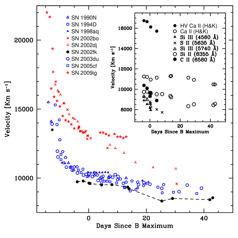
Figure 12: Time evolution of the photospheric expansion velocity derived from Si II $\lambda 6355$. Red simbols correspond to HVG SNe and blue simbols to LVG SNe. Black dots correspond to SN 2002fk, the black asterisc is the velocity of Si II $\lambda 16~{}910$ obtained by Marion et al. (2003) from a near-IR spectrum taken 12 days before maximum. In the inset we show the time evolution of other optical lines in SN 2002fk.

In Figure 12 we show the photospheric expansion velocity of SN 2002fk measured from the minimum of the Si II $\lambda 6355$ line, and a comparison with other SNe Ia. The Si II $\lambda 6355$ line is thought to trace the position of the photosphere (Benetti et al., 2005). In red we plot three HVG SNe: SN 2002bo (Benetti et al., 2004), SN 2002dj (Pignata et al., 2008) and SN 2009ig (Foley et al., 2012a; Marion et al., 2013). In blue we show the five best observed LVG SNe: SN 1990N (Leibundgut et al., 1991), SN 1994D (Patat et al., 1996), SN 1998aq (Branch et al., 2003), SN 2003du (Stanishev et al., 2007) and SN 2005cf (Wang et al., 2009). For SN 2002fk we measure a velocity gradient of $\dot{v}=26.3$ km s^-1 day^-1 between $-4$ and $+14$ days since maximum, which falls in the low end of the distribution of SNe Ia (Benetti et al., 2005). We also measure the velocity ten days after maximum $v_{10}$ $\sim$ 9,400 km s^-1. Compared to the Benetti et al. (2005) sample, SN 2002fk falls  $3\sigma$ below the mean (<$v_{10}$>$\sim$10,300 km s^-1 $\pm$ 300 km s^-1). From $\dot{v}$ and $v_{10}$ we unambiguously classify SN 2002fk as a LVG SN. Note that in the sample of near-IR spectra of SNe Ia presented by Marion et al. (2003), SN 2002fk also stands out for its anomalously low velocity measured from the Mg II $\lambda~{}10910$ absorption.

In the inset of Figure 12 we show velocities measured from other prominent lines in the spectrum. Compared to Si II $\lambda 6355$, the Si III $\lambda 4560$, S II $\lambda 5635$, and Si III $\lambda 5740$ lines show lower velocities and higher velocity gradients, implying that they form below and recede faster into the SN ejecta. We observe that Ca II $H\&K$ possibly has two components (see Section 4.4 for a detailed discussion). The main photospheric absorption is located at $v\sim$ 11,150 km s^-1 and shows a flat evolution compared to Si II $\lambda 6355$. It is possible that a detached high–velocity Ca II component is observed four days before maximum with $v\sim$ 16,700 km s^-1, and could be observed on day +5 with $v\sim$ 15,700 km s^-1 (see Figure 10). This is similar to the velocity evolution of the Ca II lines in HVG SNe.

Before maximum light the minimum of the C II $\lambda 6580$ absorption line is formed at higher velocites than Si II $\lambda 6355$ (i.e. at larger radii in the SN ejecta), but near maximum light and thereafter the C II absorption minimum is measured deeper in the ejecta than Si II. This means that there is a significant amount of unburned C II at the same position, in velocity space, where the intermediate mass elements (IME) are located. The absorption minimum of C II $\lambda 6580$ goes deeper in the ejecta with time, which could be due to emission coming from the red side of the Si II $\lambda 6355$ line (see Folatelli et al., 2012). Although the velocity estimation from the minimum of the C II lines has larger associated uncertainties owing to the weakness of the lines, the fact that both the C II $\lambda 6580$ and $\lambda 7234$ lines have similar velocities suggests that our measurements are correct. Previous studies of Parrent et al. (2011) and Folatelli et al. (2012) have shown that the C II $\lambda 6580$ line is found at higher velocities than the Si II $\lambda 6355$ line, and the velocity gradient of these two lines is roughly the same (i.e. they are parallel in velocity versus time since maximum), which is different from what we observe in SN 2002fk.

4.3 Presence of Unburned Material

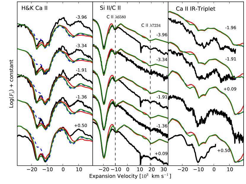
Figure 13: SYN++ models of the SN 2002fk spectra. Data are shown in black. Left panel: The blue–dashed lines correspond to models of $H\&K$ Ca II lines using $T_{exc}$ of Si II $\sim 12,500~{}K$, which is close to $T_{phot}$, with no HV Ca II component. In red we show models using $T_{exc}$ of Si II $\sim 7,000~{}K$, and in green we show models using $T_{exc}$ of Si II $\sim 12,500~{}K$, which is close to $T_{phot}$, and including a HV Ca II component. The x–axis is the expansion velocity measured with respect to the $H\&K$ Ca II line. Middle panel: in red we show models using $T_{exc}$ of Si II $\sim 7,000~{}K$. In green we show models using $T_{exc}$ of Si II $\sim 12,500~{}K$, which is close to $T_{phot}$, and including a HV C II component to get a better fit to the red side of the Si II line. The x–axis is the velocity measured with respect to C II $\lambda 6580$. Right panel: as in the left panel but for the Ca II IR–triplet. The x–axis is the expansion velocity measured with respect to the Ca II triplet. The phase of each spectrum is on the right side of each panel.

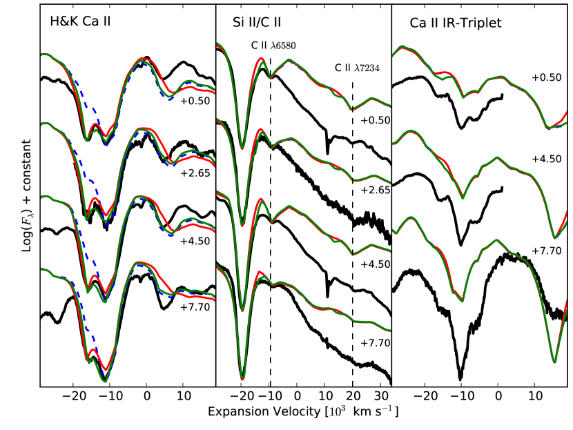
Figure 14: SYN++ models of the SN 2002fk spectra. In all three panels we show the same models as in Figure 13 but for later phases. The phase of each spectrum is on the right side of each panel.

Nearly 30% of all SNe Ia show evidence of C II $\lambda 6580$ before maximum (Parrent et al., 2011; Thomas et al., 2011b; Folatelli et al., 2012; Silverman & Filippenko, 2012b). In the middle panels of Figures 13 and 14 we present a series of spectra of SN 2002fk from $-3.96$ to $+7.70$ days since $B$–band maximum. The x–axis shows the expansion velocity measured with respect to C II $\lambda 6580$. The presence of C II is confirmed by the simultaneous detection of C II $\lambda 6580$ and $\lambda 7234$ lines at the same expansion velocities ($\sim$ 10,000 km s^-1). The detection of both lines at several epochs, together with a possible detection of C II $\lambda 4745$ in our first two epochs with a similar velocity, gives us confidence in identifying these features as C II.

Both C II $\lambda 6580$ and $\lambda 7234$ become weaker and shift to the red with time. Our latest detection of C II $\lambda 7234$ is at $+4.50$ days past B maximum while the C II $\lambda 6580$ absorption is detectable even at $+8.07$ days. Notably, this is the latest detection of C II in a normal SN Ia and, as discussed in Section 4.2, it is clear indication of the presence of unburned material mixed with IME’s if a homologous expansion of the ejecta is assumed.

4.4 Spectral Modeling

We used SYN++ (Thomas et al., 2011a), an updated version of SYNOW (Fisher et al., 1997) written in C++, to model the spectra. We modeled our data, CfA, and BSNIP spectra from $-3.96$ to $+7.70$ days since maximum.

In SYN++, one computes a spectrum by specifying the location and optical depth for a given set of ions. The input parameters for SYN++ are the photospheric velocity, the optical depth, the e-folding length of the opacity profile, the maximum and minimum cut–off velocity for each ion, and the Boltzmann excitation temperature for parameterizing line strengths.

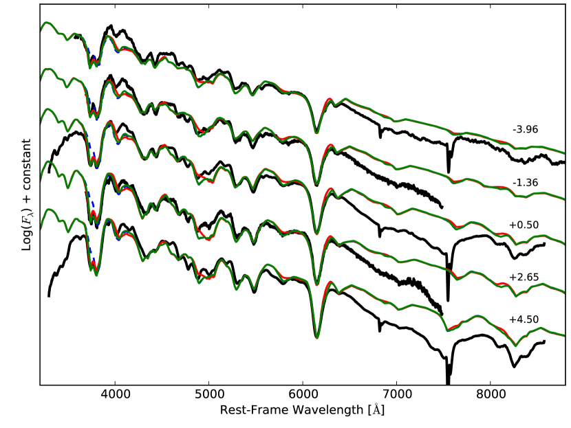
Figure 15: SYN++ models of the observed spectra of SN 2002fk spectra, shown in black. The blue–dashed lines correspond to models using $T_{exc}$ of Si II $\sim 12,500~{}K$ with no HV components. In red we show models using $T_{exc}$ of Si II $\sim 7,000~{}K$ with no HV components, and in green we show models using $T_{exc}$ of Si II $\sim 12,500~{}K$, and including HV components of Ca II, and C II. These are the same models of Figure 13, now showing the full spectral range for representative phases. The phase of each spectrum is on the right side.

Recently Foley (2013) presented convincing evidence, though not definitive, that the absorption on the blue side of the $H\&K$ Ca II line could be produced by Si II $\lambda 3858$, challenging the traditional interpretation that this absorption is caused by a HV Ca II line. Here we attempt to test both hypotheses. To do this we fit a SYN++ model to all the spectra from $-3.96$ to $+7.70$ days since $B$–band maximum. In Figure 15 we present some examples of our models which overall provide good fits to the observed spectra. We began our modeling by fitting only the photospheric lines, especially Si II and Ca II. The characteristic blackbody temperature ($T_{phot}$) in our models was $\sim 12,800~{}K$, and we set the excitation temperature ($T_{exc}$) of most of the ions at $500~{}K$ below $T_{phot}$. For the high ionizaton lines like Si III and Fe III we set $T_{exc}$ to be the same as $T_{phot}$. Then, in order to get a good fit to the absorption on the blue side of the $H\&K$ line without appealing to a HV Ca II line, we had to modify $T_{exc}$ for Si II to $\sim 7000~{}K$. We note that small variations around this value can change dramatically the strength of Si II $\lambda 3858$ but not the strength of Si II $\lambda 6355$. Alternatively, we also modeled this feature by adding a HV Ca II component with $T_{exc}$ set equal to the rest of the ions without modifying the rest of the parameters. Both approaches produce equally good models (see Figures 13, 14, and 15).

The Foley (2013) approach requires fewer parameters and reproduces the observations equally well. Remarkably, the velocity and optical depth of Si II $\lambda 6355$ proved quite insensitive to $T_{exc}$. However, the low $T_{exc}$ required to fit the Si II $\lambda 3858$ line seems slighty odd for a relatively bright SN with low R(Si II) (i.e. hot ejecta) and high ionization lines like Si III and Fe III. Additionally, there is strong evidence that supports the presence of HV Ca II in “normal” SNe Ia (Kasen et al., 2003; Gerardy et al., 2004; Mazzali et al, 2005; Stanishev et al., 2007; Tanaka et al., 2008; Childress et al., 2014). These features are clearly observed at very early phases ($\sim-7$ days) in both Ca II $H\&K$ and the Ca II IR–triplet, but near maximum they are not always easy to identify (Mazzali et al, 2005). We conclude that, while both Si II $\lambda 3858$ and HV Ca II produce equally good fits to the data within the SYN++ framework, more realistic radiative transfer models will be necessary to distinguish which line is responsible for the absorption on the blue side of the $H\&K$ line.

As can be seen in Figures 13 and 14, the red side of the Si II $\lambda 6355$ profile is not properly fit by Si II alone (shown in red). To obtain a better fit we added a C II HV component (shown in green). In the case of our spectra, which are not corrected for telluric absorption, this feature on the red side of the Si II profile could be due to the lack of such corrections. However, the CfA spectra obtained on days -3.34 and -1.36, which do include corrections for telluric lines, are best modelled with a HV C II component. Interestingly, the HV C II is at nearly the same velocity of the HV Ca II ($\sim$ 16,000 km s^-1). The presence of a HV C II was previously suggested by Fisher et al. (1997), and is not completely unexpected since unburned carbon material should be present in the outer layers of SNe Ia. We flag the presence of HV C II as possible but not as certain.

5 DETERMINATION OF THE HUBBLE CONSTANT USING THE CEPHEID DISTANCE TO NGC 1309

With the relative Cepheid distance between NGC 1309 and NGC 4258 of Riess et al. (2011a) ($\mu_{NGC~{}1309}-\mu_{NGC~{}4258}=3.276\pm 0.05$), the maser distance to NGC 4258 of Humphreys et al. (2013) ($\mu_{NGC~{}4258}=29.40\pm 0.06$), the peak brightness and reddening of SN 2002fk derived in Section 3.3, it is straightforward to calculate the Hubble constant ($H_{0}$) via the formula $H_{0}=10^{0.2(M_{max}^{1.1}+25-\alpha)}$, where $M_{max}^{1.1}$ is the absolute magnitude of SN 2002fk corrected for reddening and $\Delta m15$, and $\alpha$ is the corresponding zero point of the Hubble diagram. In the optical ($BVI$), we adopt the decline rate versus luminosity ($\Delta m15$/$M_{max}$) relations and zero points from Phillips et al. (1999), who employ the same prescription that we use here for luminosity and reddening corrections. In the near-IR ($JHK$) we adopt $\Delta m15$/$M_{max}$ relations and zero points derived from two independent analysis of nearly the same near-IR CSP observations, one by Folatelli et al. (2010) and the other by Kattner et al. (2012).

In Table 10 we summarize all the adopted parameters and the resulting values for $H_{0}$. The statistical uncertainty in $H_{0}$ was computed from a Monte Carlo simulation. Our code computes $10,000$ simulated values of $H_{0}$ assuming a Gaussian distribution in peak magnitude, reddening, $\Delta m15$, the slope of the $\Delta m15$/$M_{max}$ relationship, and the zero point of the Hubble diagram. The systematic error includes 0.08 mag in distance modulus to NGC 1309, 0.03 mag in the photometric zero point, and the intrinsic dispersion in the $\Delta m15$/$M_{max}$ relationship from Phillips et al. (1999), Folatelli et al. (2010), and Kattner et al. (2012).

As can be seen in Table 10, the $H_{0}$ values that we derive from the optical bands ($BVI$) are very consistent with each other, allowing us to combine them into an $BVI$ average of $H_{0}(BVI)=69.6\pm{2.1}~{}(\pm 5.0$ systematic) km s^-1 Mpc${}^{-1}~{}$, where the systematic error includes 0.08 mag in distance modulus to NGC 1309, 0.03 mag in the photometric zero point, and the intrinsic dispersion in the $\Delta m15$/$M_{max}$ relationship including the variance in each band and band-to-band covariances. Our value is 0.8 $\sigma$ lower than the one published by Riess et al. (2011a), $H_{0}=73.8\pm{2.4}$ km s^-1 Mpc${}^{-1}~{}$, from eight SNe Ia with precise Cepheid distances. This is due to the fact that SN 2002fk lies in the bright side of their luminosity distribution. In fact, using the values listed in Table 3 of Riess et al. (2011a) and their Eq. (4), we find $H_{0}=68.5$ km s^-1 Mpc${}^{-1}~{}$for this same SN, in very good agreement with our determination. Thus, using SN 2002fk alone to determine $H_{0}$ is expected to yield a lower value than the fit to all eight SNe in their sample.

Table 10 shows that our near-IR estimate of $H_{0}$ is sensitive to the adopted calibration: using Kattner et al. (2012), we obtain $H_{0}(JH)=66.7\pm{1.0}~{}(\pm 3.5$ systematic) km s^-1 Mpc${}^{-1}~{}$, whereas if we employ Folatelli et al. (2010) we get $H_{0}(JHK)=63.0\pm{0.8}~{}(\pm 2.8$ systematic) km s^-1 Mpc${}^{-1}~{}$. This discrepancy is mainly due to the different zero points obtained from their analysis, 0.17 and 0.07 mag in $J$ and $H$, respectively (see Table 10), which arise from the different techniques employed to measure peak magnitudes. While Kattner et al. (2012) directly measured peak magnitudes based on a cubic-spline interpolation to seven exquisitely observed SNe with observations starting before maximum, Folatelli et al. (2010) included peak magnitudes extrapolated from a template light curve fit. As mentioned by Kattner et al. (2012) the large diversity in early time near-IR light curve shapes can lead to significant errors when fitting template light curves to derive peak brightnesses.

Despite the differences in $H_{0}$ caused by the near-IR calibration adopted, it appears that the near-IR yields somewhat lower (6-9%) $H_{0}$ values than the optical. How significant is this difference? Given that the systematic error for this particular SN is almost fully correlated band to band (owing to the same Cepheid distance and the fact that the intrinsic dispersion of SNe Ia is correlated band to band), the significance can be estimated from the statistical uncertainty alone, which yields 1.2 and 2.9 $\sigma$ for Kattner et al. (2012) and Folatelli et al. (2010), respectively. It will be essential to further examine this issue by expanding the sample of near-IR SN light curves with good sampling near maximum, which should lead to a more robust determination of the zero point of the Hubble diagram and the $\Delta m15$/$M_{max}$ relationship. Such effort should be rewarded with a significantly more precise determination of $H_{0}$: as can be seen in Table 10, the near-IR yields smaller statistical uncertainties due to a smaller sensitivity to extinction, decline rate correction, and higher precision in the zero point of the Hubble diagram. As opposed to the optical bands where the zero point is subject to inaccuracies caused by the heterogeneity in the various photometric systems employed, our near-IR zero point is based in a single homogeneous Carnegie photometric dataset, an essential ingredient in lowering the statistical uncertainty in $H_{0}$.

An independent value of $H_{0}=69.77^{+2.07}_{-2.07}$ was obtained by Sullivan et al. (2011) by combining the SNLS3 data with the full WMAP7 power spectrum and the Sloan Digital Sky Survey luminous red galaxy power spectrum (DR7). Similarly, Mehta et al. (2012) obtained $H_{0}=69.8\pm 1.2$ by fitting a $\Lambda CDM$ model to the DR7 and WMAP7 data. Studies of galaxy clustering from the SDSS–III Data Release 8 (DR8) yield $H_{0}=70.5\pm 1.6$ (Ho et al., 2012). More recently, the first results based on the Planck satellite measurements of the CMB temperature and lensing-potential power spectra find a low value of $H_{0}=67.3\pm 1.2$ (Ade et al., 2014). All these experiments reveal some tension with the $H_{0}=73.8\pm 2.4$ value obtained by Riess et al. (2011a). Our analysis provides the first determination of $H_{0}$ from near-IR SNe Ia data, and suggests that the near-IR could help to alleviate this tension.

6 DISCUSSION AND CONCLUSIONS

We present early and complete optical ($BVRI$) and near-IR ($JHK$) light-curves of SN 2002fk starting 12 days before maximum light through 122 days past maximum, along with a series of 15 optical spectra from -4 to +95 days since maximum. Our study reveals the following distinguishing properties of SN 2002fk:

$\bullet$ Low decline rate ($\Delta m15$=1.02) of the B lightcurve, consistent with a higher than average peak luminosity ($M_{B}$=-19.49).

$\bullet$ Negligible host galaxy reddening as inferred from the observed colors.

$\bullet$ Slightly bluer than average $B-V$ color near maximum.

$\bullet$ Presence of Si II 6355 with a relatively low (9,500 km s${}^{-1}~{}$) expansion velocity near maximum, and a small velocity gradient, $\dot{v}_{Si~{}II}=26$ km s^-1 day^-1.

$\bullet$ Blue $U-B$ and a red $V-I$ early-time color, expected for LVG SNe Ia (Cartier et al., 2011).

$\bullet$ Presence of C II lines in the early-time spectra expanding at  11,000 km s${}^{-1}~{}$persisting until  8 days past maximum light with a velocity $\sim$9,000 km s${}^{-1}~{}$, and possible HV component with 16,000 km s${}^{-1}~{}$.

$\bullet$ Possible presence of a HV Ca II $H\&K$ component in the early-time spectra expanding at $\sim 16,000$ km s${}^{-1}~{}$and persisting until $\sim$ 8 days past maximum, with similar velocity of a possible HV C II component (an alternative explanation for the HV Ca II is Si II $\lambda 3858$; see Foley, 2013).

In the off-center explosion models of Maeda et al. (2010c), SNe Ia with low Si II velocity gradients are those with the ignition region oriented towards the observer. Therefore, we expect a negative (blueshifted) velocity shifts of the [Fe II] $\lambda 7155$ and [Ni II] $\lambda 7378$ nebular lines ($V_{neb}$). Silverman et al. (2013) have recently shown that this is indeed the case for SN 2002fk ($V_{neb}=-2060$ km s${}^{-1}~{}$), lending support to the Maeda et al. (2010c) models, the Cartier et al. (2011) relations (see their Fig. 2), and Förster et al. (2012) work. Parrent et al. (2011) and Folatelli et al. (2012) have noted that SNe showing C II in their spectra are grouped preferentially in the bottom of the Si II expansion velocity distribution. Our observations of SN 2002fk are consistent with such findings. The connection between viewing angle of an off-center explosion and the presence of C II in the early time spectrum suggests that the observation of C II could be also due to a viewing angle effect. A possible explanation could be that when the ignition region is directed towards us, the burning front leaves some pockets of unburned material in the direction of the observer. Our observations indicate also that SN 2002fk is quite luminous and somewhat bluer than normal, which might also be a signature of an ignition region oriented towards the observer.

The possible presence of a HV Ca II component in the early-time spectra expanding at $\sim 16,000$ km s${}^{-1}~{}$persisting until $\sim$ 8 days past maximum, at a similar velocity of a possible detection of a HV C II component, suggests that these HV features may arise from density enhanced regions containing a mixture of Ca II and C II.

Our photometry shows good agreement with the optical magnitudes published by Riess et al. (2009b), except in the $I$-band where we find an offset of 0.07 mag. We do not have an explanation for this worrisome discrepancy except that LOSS employed an $I$ filter with an extended red tail compared to the standard bandpass.

Adopting the Cepheid distance to NGC 1309 recently measured by Riess et al. (2011a) and Humphreys et al. (2013), we derive optical and near-IR absolute magnitudes for SN 2002fk. Using the $BVI$ absolute magnitude/decline rate calibration of Phillips et al. (1999) we solve for the Hubble constant, obtaining a consistent value of $H_{0}=69.6\pm 2.1$ ($\pm~{}5.0$ systematic), which is 0.8 $\sigma$ lower than the one published by Riess et al. (2011a), $H_{0}=73.8\pm 2.4$ from eight SNe Ia with precise Cepheid distances. This is due to the fact that SN 2002fk lies on the bright side of their luminosity distribution.

We proceed in a similar manner for the $JHK$ absolute magnitudes to derive the first $H_{0}$ value based on near-IR measurements of a SN Ia. As opposed to the optical method that relies on many different photometric calibrations containing significant systematic differences (as shown in Appendix B), the near-IR has the great advantage that it is founded on a homogeneous Carnegie photometric dataset including (1) the Persson standards (Persson et al., 2002), (2) the CSP Hubble diagram (Folatelli et al., 2010; Kattner et al., 2012), and (3) the calibrating CATS SN 2002fk. Our near-IR $H_{0}$ values rely on two CSP different absolute magnitude/decline rate relationships. Using the Kattner et al. (2012) relation, we obtain $H_{0}(JH)=66.7\pm{1.0}~{}(\pm 3.5$ systematic) km s^-1 Mpc${}^{-1}~{}$, whereas employing Folatelli et al. (2010) we get $H_{0}(JHK)=63.0\pm{0.8}~{}(\pm 2.8$ systematic) km s^-1 Mpc${}^{-1}~{}$. This discrepancy is mainly due to the different zero points obtained from their analysis, 0.17 and 0.07 mag in $J$ and $H$, respectively, which arise from the different techniques employed to measure peak magnitudes. More importantly, it appears that the near-IR yields somewhat lower (6-9%) $H_{0}$ values than the optical, with a significance of 1.2 and 2.9 $\sigma$ depending on the near-IR calibration adopted. It is essential to further examine this issue by (1) expanding the sample of high-quality near-IR light curves of SNe in the Hubble flow, and (2) increasing the number of nearby SNe with near-IR SN light curves and precise Cepheid distances, which affords the promise to deliver a more precise determination of $H_{0}$.

Appendix A CROSS-CAMERA SUBTRACTIONS

Since our template images in $UBVRI$ were acquired with a different instrument than the ones used for the SN imaging (see Table 1), there is a potential systematic error caused by our cross-camera subtractions. To assess this error we performed the following intrepid test: we subtracted the $V$ template from the $B$ SN images, the $B$ template from the $V$ SN images, the $V$ template from the $R$ SN images, and the $R$ template from the $I$ SN images. Then we measured instrumental magnitudes with a 3 arcsec aperture both in the crossed subtracted images and those performed with the same filter. The magnitude differences yielded by this test amounted to 0.001-0.003 mag. Given that these cross subtractions involve wavelength differences $\sim$1,000 Å between templates and SN images, the actual error caused by using templates that differ by $\sim$10 Å in central wavelenghts (as in our case) from the SN images can be ignored. In the near-IR this potential uncertainty does not exist because the templates images were obtained with the same instrument employed for the SN.

Appendix B LOCAL STANDARDS & PHOTOMETRIC ZERO POINTS

Given that there are other sources of optical photometry available in the literature for SN 2002fk, it is necessary to verify the compatibility of the individual photometric calibrations before attempting to merge the photometry. Initially we started this exercise by comparing the magnitudes of the four local standard stars in common (stars 5, 6, 7, 8) between us (LCO/Swope) and LOSS. To our surprise we discovered very good agreement in BVR but a significant systematic offset $\sim$0.07 mag in the $I$-band. When we noticed this discrepancy, we proceeded to obtain additional measurements of the local standards with the CTIO/0.9-m telescope (two nights) and the CTIO/PROMPT telescopes (two nights) under photometric conditions. Given that we found very good agreement ($\leq$0.015 mag) in $BVRI$ among all three calibrations and a reasonable ($\sim$0.06 mag) consistency in the $U$-band between LCO/Swope and CTIO/0.9–m (no $U$ measurements could be obtained with CTIO/PROMPT) we decided to combine all of our $UBVRI$ values into the single CATS calibration, which is presented in Table 3.

Our internal consistency can be seen in detail in Table 8 which summarizes the differences in each filter between the magnitudes of the local standard stars measured with our three instruments (LCO/Swope, CTIO/0.9-m, CTIO/PROMPT) and our average CATS calibration. We find excellent agreement in $BVRI$ ($\leq$0.015 mag). This is remarkable considering that the CTIO/PROMPT data were reduced with a completely independent pipeline by one of us (GP). In the $U$-band the $\sim$0.06 mag difference between LCO/Swope and CTIO/0.9–m (no $U$ measurements could be obtained with CTIO/PROMPT) is not surprising given that $U$–band photometry is generally difficult to calibrate as a result of filter mismatches or differences in the sky transmission (i.e. effective bandpass), and large systematic differences are common.

Having demonstrated our own internal consistency (with the above mentioned caveat in $U$) we return to the issue of comparing our photometry with the external measurements of the local standards obtained by LOSS (Riess et al., 2009b; Ganeshalingam et al., 2010) and CfA3 (Hicken et al., 2009). This comparison is presented in Table 8 which gives magnitude differences between the local standard stars measured by CATS, LOSS, and CfA3. Overall we found good agreement between LOSS and CATS ($\leq$0.02 mag), with the notable exception of the $I$-band where the LOSS magnitudes are systematically brighter by $\sim 0.07$ mag. We do not have an explanation for this worrisome discrepancy except that LOSS employed on the Nickel telescope an $I$ filter with an extended red tail compared to the standard bandpass [see Fig. 1 in Ganeshalingam et al. (2010)]. Perhaps this is also the cause of the systematic differences $\sim$0.1 mag in the $I$–band between LOSS and CfA2 (Jha et al., 2006) reported by Ganeshalingam et al. (2010) for some SNe. When we compare CATS and CfA3, we find better agreement in $I$ (CfA3 is between CATS and LOSS). However, what is more concerning is that CfA3 is consistently brighter than CATS by $\sim 0.03-0.04$ mag in all $UBVRI$ filters. While LOSS is halfway between CATS and CfA3 in $B$, LOSS is much closer to CATS than CfA3 in $V$ and $R$. We cannot claim which one is correct, but the advantage of the CATS calibration is that it was obtained with three different cameras, two independent pipelines, and two reducers.

Based on this analysis, we adopt a systematic uncertainty of $0.03$ mag for our photometric zero points. Unfortunately, we cannot apply this approach to the near-IR because the 2MASS magnitudes are not sufficiently precise. Hence, we adopt the same uncertainty of $0.03$ mag.

Appendix C S-CORRECTIONS

SN magnitudes obtained with different instruments can potentally lead to significant systematic errors due to the non-stellar nature of the SN spectrum. These effects, a.k.a. S-terms, were computed by Stritzinger et al. (2002) for the normal Type Ia SN 1999ee. As shown in their Fig. 4, the S-corrections change with time as the SN spectrum evolves. The systematic errors for the CTIO/0.9-m camera are generally small in $BVRI$, from 0.01 mag near maximum to 0.04 mag at late times ($\sim$60 days past maximum), suggesting that this instrument provides a good match to the standard system (Bessell, 1990), while for the YALO instrument the systematic errors are larger ($\sim$0.05-0.08 mag) owing to significant instrumental departures from the standard bandpasses. In order to quantify this effect in SN 2002fk, we took advantage of the fact that the object was measured with seven different instruments allowing us to calculate magnitude differences among all of them after removing the systematic differences caused by the photometric zero-points. This empirical approach showed that the S-terms amount to 0.02 mag at maximum light and 0.03 mag at later epochs (40-80 days after peak), allowing us to to attach a systematic error to our $BVRI$ photometry. Its is encouraging that this empirical approach yields similar values to those computed by Stritzinger et al. (2002) for the CTIO/0.9-m camera. Likewise, in the near-IR we estimate the systematic errors caused by the S-terms to be 0.02 mag at maximum, from a comparison of the SN magnitudes measured with Baade/Classic-Cam and du Pont/WIRC. We cannot apply this technique at later times in the near-IR since SN 2002fk was observed with a single instrument, but we can safely adopt the 0.03 uncertainty measured in the optical. Most likely, this is an upper limit to the systematic errors in the near-IR, considering that the instrument detector and filters used with WIRC and Classic-Cam were essentially the same as those employed by Persson et al. (1998) in the establishment of the standard system.

Table 1: Photometric Observations of SN 2002fk.

Observatory	Telescope	Instrument	Detector	Plate Scale	Filters
				(arcsec pixel-1)
LCO	Swope	CCD	SITe 2048$\times$3150	0.435	$UBV(RI)_{KC}$
LCO	du Pont	WFCCD	Tek 2048$\times$2048	0.774	$BV(I)_{KC}$
LCO	du Pont	CCD	Tek 2048$\times$2048	0.259	$UBV(RI)_{KC}$
LCO	Baade	LDSS-2	SITe 2048$\times$2048	0.380	$BV(R)_{KC}$
CTIO	0.9m	CCD	2048$\times$2048	0.396	$UBV(RI)_{KC}$
CTIO	1.5m	CCD	2048$\times$2048	0.440	$BV(RI)_{KC}$
CTIO	PROMPT	CCD	Alta U47 E2V 1024$\times$1024	0.600	$BV(RI)_{KC}$
LCO	du Pont	WIRC	HAWAII-1 1024$\times$1024	0.196	$J_{S}HK_{S}$
LCO	Baade	Classic-Cam	NICMOS3 256$\times$256	0.094	$J_{S}HK_{S}$

Table 2: Spectroscopic Observations of SN 2002fk.

Date(UT)	JD	Phase	Instrument/	Wavelength	Resolution	Exposure
	-2,400,000	(days)	Telescope	Range (Å)	(Å)	(s)
2002 Sep 26	52543.84	-3.96	LDSS-2/Baade	3600 - 9000	14	120
2002 Sep 28	52545.89	-1.91	LDSS-2/Baade	3600 - 9000	14	200
2002 Sep 30	52547.89	0.09	WFCCD/du Pont	3800 - 9200	8	200
2002 Oct 01	52548.31	0.50	FORS1-PMOS/VLT	3330 - 8500	12	2880
2002 Oct 05	52552.32	4.50	FORS1-PMOS/VLT	3330 - 8500	12	2880
2002 Oct 08	52555.87	8.07	WFCCD/du Pont	3800 - 9200	8	200
2002 Oct 14	52561.36	13.54	FORS1-PMOS/VLT	3330 - 8500	12	2400
2002 Oct 14	52561.83	14.03	LDSS-2/Baade	3600 - 9000	14	60
2002 Oct 25	52573.15	25.35	LDSS-2/Baade	3600 - 9000	14	120
2002 Oct 29	52576.87	29.07	LDSS-2/Baade	3600 - 9000	14	90
2002 Nov 11	52589.82	42.02	B&C Spec./Baade	3200 - 9200	7	300
2002 Nov 12	52590.83	43.03	B&C Spec./Baade	3200 - 9200	7	200
2002 Nov 28	52606.75	58.95	B&C Spec./Baade	3200 - 9200	7	200
2002 Dec 02	52610.70	62.90	WFCCD/du Pont	3800 - 9200	8	450
2003 Jan 03	52642.73	94.93	Mod. Spec./du Pont	3790 - 7270	7	450

Table 3: $UBRVI$ Photometric Sequence Around SN 2002fk.

Star	$U$	$N$	$B$	$N$	$V$	$N$	$R$	$N$	$I$	$N$	LOSS	CfA3
											name	name
c1	13.604(0.018)	4	13.424(0.016)	4	12.705(0.014)	4	12.322(0.015)	4	11.951(0.014)	4	-	-
c2	14.337(0.020)	4	13.386(0.016)	4	12.346(0.014)	4	11.752(0.015)	4	11.279(0.014)	4	-	-
c3	13.248(0.013)	4	13.278(0.025)	4	12.718(0.014)	4	12.366(0.016)	4	12.065(0.014)	4	-	-
c4	14.313(0.014)	4	14.230(0.019)	4	13.620(0.013)	4	13.281(0.008)	4	12.961(0.008)	4	-	-
c5	16.197(0.009)	6	16.330(0.013)	8	15.771(0.006)	8	15.424(0.007)	8	15.077(0.005)	8	4	4
c6	16.419(0.010)	6	16.437(0.013)	8	15.820(0.006)	8	15.447(0.006)	8	15.080(0.006)	8	2	5
c7	16.209(0.011)	6	16.276(0.008)	8	15.759(0.005)	8	15.429(0.010)	8	15.102(0.006)	8	1	6
c8	17.519(0.018)	6	17.555(0.013)	8	16.948(0.008)	8	16.595(0.007)	8	16.237(0.008)	8	3	3
c9	$\cdots$	4	19.083(0.028)	4	17.842(0.021)	4	17.069(0.010)	4	16.425(0.007)	4	-	-
c10	$\cdots$	4	16.329(0.016)	4	15.780(0.014)	4	15.425(0.015)	4	15.122(0.010)	4	-	-
c11	$\cdots$	4	15.221(0.016)	4	14.669(0.014)	4	14.310(0.015)	4	14.013(0.010)	4	-	-

Note. — Errors given in parenthesis, are 1$\sigma$ statistical uncertainties. For each star we indicate N, the number of photometric nights used to calibrate them.

Table 4: Color Terms for the five Optical Cameras

Telescope	$U$	$B$	$V$	$R$	$I$
Swope/CCD	+0.177	+0.053	-0.054	+0.021	+0.052
du Pont/WFCCD	$\cdots$	+0.125	-0.045	$\cdots$	+0.010
Clay/LDDS-2	$\cdots$	+0.132	+0.046	$\cdots$	$\cdots$
CTIO 0.9-m/CCD	+0.126	-0.086	+0.011	+0.004	+0.007
CTIO 1.5-m/CCD	+0.139	-0.080	+0.030	+0.016	+0.017

Note. — Color terms are defined in equations 1-5.

Table 5: $UBVRI$ Photometry of SN 2002fk.

Date(UT)	JD-2,400,000	$U$	$B$	$V$	$R$	$I$	Telescope
2002 Sep 21	52538.8	13.523(0.013)	14.128(0.016)	14.234(0.014)	14.149(0.015)	14.119(0.010)	Swope
2002 Sep 26	52543.9	$\cdots$	13.443(0.012)	13.515(0.014)	$\cdots$	$\cdots$	Baade
2002 Sep 30	52547.9	$\cdots$	13.319(0.047)	13.358(0.019)	$\cdots$	13.609(0.051)	du Pont
2002 Oct 01	52548.9	12.792(0.018)	13.287(0.016)	13.350(0.014)	13.335(0.011)	13.595(0.014)	Swope
2002 Oct 08	52555.9	$\cdots$	13.675(0.076)	13.623(0.085)	$\cdots$	14.003(0.074)	du Pont
2002 Oct 14	52561.8	$\cdots$	14.261(0.017)	13.904(0.014)	$\cdots$	$\cdots$	Baade
2002 Oct 20	52567.8	15.044(0.010)	14.883(0.011)	14.239(0.010)	14.133(0.011)	14.181(0.010)	Swope
2002 Oct 21	52568.8	15.195(0.024)	15.014(0.011)	14.355(0.023)	14.139(0.013)	14.218(0.023)	Swope
2002 Oct 24	52571.9	15.544(0.017)	15.294(0.014)	14.409(0.015)	14.196(0.015)	14.198(0.015)	CTIO 0.9-m
2002 Oct 25	52572.8	15.631(0.018)	15.394(0.016)	14.500(0.014)	14.205(0.015)	14.121(0.014)	Swope
2002 Oct 29	52572.9	$\cdots$	$\cdots$	14.511(0.014)	$\cdots$	$\cdots$	Baade
2002 Oct 30	52576.9	$\cdots$	15.782(0.018)	14.714(0.010)	14.376(0.014)	$\cdots$	Baade
2002 Oct 08	52577.9	$\cdots$	15.825(0.017)	14.778(0.019)	$\cdots$	14.123(0.017)	du Pont
2002 Nov 07	52585.8	16.388(0.018)	16.238(0.016)	15.229(0.014)	14.888(0.015)	14.539(0.015)	Swope
2002 Nov 08	52586.9	$\cdots$	16.277(0.016)	15.256(0.014)	14.939(0.015)	14.570(0.019)	Swope
2002 Nov 12	52590.8	16.531(0.020)	16.396(0.016)	15.440(0.014)	15.129(0.015)	14.840(0.014)	Swope
2002 Nov 18	52596.7	16.668(0.019)	16.546(0.016)	15.640(0.014)	15.358(0.015)	15.161(0.014)	Swope
2002 Dec 02	52610.7	$\cdots$	16.819(0.062)	16.075(0.033)	$\cdots$	15.785(0.019)	du Pont
2002 Dec 04	52612.8	17.045(0.023)	16.830(0.016)	16.091(0.014)	15.922(0.015)	15.887(0.014)	Swope
2002 Dec 07	52615.7	17.043(0.018)	16.848(0.016)	16.128(0.014)	15.981(0.015)	16.000(0.014)	Swope
2003 Jan 07	52646.7	17.803(0.024)	17.324(0.016)	16.907(0.010)	16.954(0.015)	17.184(0.014)	Swope
2003 Jan 31	52670.6	$\cdots$	17.762(0.014)	17.397(0.015)	17.633(0.015)	18.069(0.027)	CTIO 1.5-m

Note. — Errors given in parenthesis, are 1$\sigma$ statistical uncertainties.

Table 6: $JHK_{s}$ Photometric Sequence Around SN 2002fk.

Star	$J$	$J_{2MASS}$	$H$	$H_{2MASS}$	$K_{s}$	$K_{2MASS}$
c5	14.599(0.014)	14.582(0.028)	14.259(0.008)	14.272(0.055)	14.148(0.009)	14.173(0.067)
c8	15.764(0.020)	15.712(0.062)	15.439(0.009)	15.564(0.101)	15.299(0.024)	15.408(0.179)
c12	16.093(0.011)	16.083(0.080)	15.439(0.009)	15.312(0.094)	15.190(0.019)	15.100(0.137)
c13	18.224(0.064)	$\cdots$	17.628(0.077)	$\cdots$	$\cdots$	$\cdots$

Note. — Errors given in parenthesis, are 1$\sigma$ statistical uncertainties.

Table 7: $JHK_{s}$ Photometry of SN 2002fk.

Date(UT)	JD-2,400,000	$J$	$H$	$K_{s}$	Telescope
2002 Sep 18	52535.7	15.162(0.011)	15.200(0.011)	15.107(0.011)	du Pont
2002 Sep 19	52536.7	14.798(0.011)	14.859(0.011)	14.797(0.011)	du Pont
2002 Sep 20	52537.8	14.540(0.011)	14.605(0.011)	14.532(0.015)	du Pont
2002 Sep 21	52538.7	14.324(0.011)	14.405(0.011)	14.323(0.011)	du Pont
2002 Sep 22	52539.7	14.132(0.011)	14.234(0.015)	14.103(0.015)	du Pont
2002 Sep 23	52540.7	14.000(0.011)	14.133(0.011)	13.997(0.011)	du Pont
2002 Sep 24	52541.7	13.860(0.016)	14.044(0.016)	13.863(0.017)	Baade
2002 Sep 24	52541.7	13.879(0.011)	14.036(0.011)	13.926(0.011)	du Pont
2002 Sep 25	52542.7	13.801(0.015)	13.975(0.011)	13.766(0.019)	Baade
2002 Sep 27	52544.7	13.764(0.015)	13.981(0.011)	13.741(0.017)	Baade
2002 Sep 29	52546.6	13.847(0.011)	14.113(0.011)	13.859(0.011)	du Pont
2002 Oct 14	52560.7	15.623(0.011)	14.590(0.011)	14.264(0.011)	du Pont
2002 Oct 15	52562.7	15.647(0.011)	14.549(0.011)	14.262(0.011)	du Pont
2002 Oct 20	52567.8	15.549(0.011)	14.332(0.011)	14.152(0.011)	du Pont
2002 Oct 23	52570.6	15.497(0.018)	$\cdots$	$\cdots$	du Pont
2002 Oct 24	52571.8	15.377(0.011)	14.175(0.011)	14.083(0.011)	du Pont
2002 Nov 12	52590.8	15.854(0.011)	14.905(0.011)	14.922(0.011)	du Pont
2002 Nov 14	52593.8	16.073(0.011)	15.030(0.011)	15.063(0.011)	du Pont
2002 Nov 19	52597.5	16.367(0.011)	15.248(0.011)	15.249(0.011)	du Pont
2002 Nov 22	52600.6	16.549(0.013)	15.367(0.014)	15.350(0.030)	du Pont
2002 Dec 09	52617.5	17.713(0.039)	16.112(0.015)	16.010(0.027)	du Pont
2002 Dec 11	52619.7	17.798(0.030)	16.185(0.011)	16.070(0.027)	du Pont
2002 Dec 23	52631.6	18.534(0.042)	16.797(0.017)	16.549(0.033)	du Pont
2003 Jan 11	52650.6	19.434(0.103)	17.597(0.027)	17.039(0.056)	du Pont

Note. — Errors given in parenthesis, are 1$\sigma$ statistical uncertainties.

Table 8: Mean Differences among different photometric systems and our Average values

	$\Delta U$	$\Delta B$	$\Delta V$	$\Delta R$	$\Delta I$
$LCO/Swope-Average\tablenotemark{a}$	$0.025\pm 0.008$	$0.009\pm 0.004$	$0.006\pm 0.006$	$0.006\pm 0.004$	$0.006\pm 0.002$
$CTIO/0.9m-Average\tablenotemark{a}$	$-0.038\pm 0.012$	$-0.006\pm 0.008$	$-0.009\pm 0.006$	$-0.004\pm 0.006$	$-0.007\pm 0.008$
$CTIO/PROMPT-Average\tablenotemark{a}$	$\cdots$	$-0.006\pm 0.028$	$-0.003\pm 0.010$	$-0.008\pm 0.012$	$-0.008\pm 0.008$
$LOSS\tablenotemark{b}-Average\tablenotemark{a}$	$\cdots$	$-0.020\pm 0.016$	$-0.001\pm 0.024$	$0.004\pm 0.026$	$-0.070\pm 0.016$
$CfA3\tablenotemark{c}-Average\tablenotemark{a}$	$-0.025\pm 0.026$	$-0.038\pm 0.022$	$-0.031\pm 0.004$	$-0.033\pm 0.004$	$-0.044\pm 0.008$
$CfA3\tablenotemark{c}-LOSS\tablenotemark{b}$	$\cdots$	$-0.017\pm 0.016$	$-0.026\pm 0.020$	$-0.037\pm 0.022$	$0.022\pm 0.022$

Note. — Quoted uncertanties are weighted standard deviations

Table 9: SN 2002fk total (Galactic + host galaxy) reddening from different methods.

Method	$E(B-V)$	Reference
$(B-V)_{Tail}$	$0.066\pm 0.019$	Phillips et al. (1999)
$B_{max}-V_{max}$	$0.009\pm 0.044$	Phillips et al. (1999)
$V_{max}-I_{max}$	$0.082\pm 0.038$	Phillips et al. (1999)
$(V-H)$	$0.014\pm 0.037$	Krisciunas et al. (2004b)
$(V-K)$	$0.075\pm 0.036$	Krisciunas et al. (2004b)
Mean	$0.057\pm 0.036$

Table 10: Hubble constant using different filter calibrations.

Filter	$m_{max}$	$M_{max}$	$M_{max}^{1.1}$	$\alpha$	$\sigma_{SN}$	$H_{0}$	Systematic	Reference
						(km s-1 Mpc${}^{-1}~{}$)	Error
$B$	13.07(0.15)	-19.49(0.17)	-19.43(0.17)	-3.671(0.043)	0.11	$70.5^{+5.4}_{-5.0}$	4.5	Phillips et al. (1999)
$V$	13.19(0.11)	-19.37(0.14)	-19.32(0.15)	-3.615(0.037)	0.09	$72.4^{+4.5}_{-4.1}$	4.1	Phillips et al. (1999)
$I$	13.47(0.07)	-19.09(0.11)	-19.06(0.08)	-3.236(0.035)	0.13	$68.3^{+2.8}_{-2.7}$	4.9	Phillips et al. (1999)
$J$	13.71(0.04)	-18.85(0.09)	-18.83(0.09)	-2.893(0.003)	0.125	$65.1^{+1.4}_{-1.3}$	4.5	Kattner et al. (2012)
$H$	13.95(0.03)	-18.61(0.08)	-18.57(0.09)	-2.733(0.009)	0.053	$68.0^{+1.4}_{-1.2}$	3.2	Kattner et al. (2012)
$J$	13.71(0.04)	-18.85(0.09)	-18.80(0.09)	-2.727(0.01)	0.12	$60.8^{+1.3}_{-1.3}$	4.1	Folatelli et al. (2010)
$H$	13.95(0.03)	-18.61(0.08)	-18.59(0.09)	-2.667(0.02)	0.16	$65.4^{+1.2}_{-1.2}$	5.5	Folatelli et al. (2010)
$K$	13.74(0.03)	-18.82(0.08)	-18.76(0.09)	-2.717(0.03)	0.10	$61.9^{+1.6}_{-1.5}$	5.4	Folatelli et al. (2010)

Figure 9: $V~{}-$ near-IR colors of SN 2002fk and the well sampled SNe Ia of similar $\Delta m15$: SN 2001el, SN 2002dj, SN 2003du, SN 2005cf and SN 2006dd. Dashed line are $V~{}-$ near-IR loci for mid-range decliners and dotted-dashed line are $V~{}-$ near-IR loci for slow decliners (Krisciunas et al., 2004b).

Figure 10: Optical spectral evolution of SN 2002fk. The spectra have been corrected for the redshift of the host galaxy (2,137 km s^-1) and have been shifted vertically for clarity. The labels on the right mark the days since B-band maximum.

Figure 11: Spectrum of SN 2002fk at -4, 0, +25 and +95 days after B maximum. We plot for comparison SN 1994D, SN 1998aq, SN 2003du, SN 2006gz, and SN 2005cf at similar epochs.

References

- Ade et al. (2014) Ade, P. A. R. et al. (Planck collaboration) 2014, å, in press
- Allington-Smith et al. (1994) Allington-Smith et al. 1994, PASP, 703, 983
- Amanullah & Goobar (2011) Amanullah, R., & Goobar, A. 2011, ApJ, 735, 20
- Ayani & Yamaoka (2002) Ayani, K., & Yamaoka, Y., 2002, IAUC 7976
- Benetti et al. (2005) Benetti, S. et al. 2005, ApJ, 623, 1011
- Benetti et al. (2004) Benetti, S. et al. 2004, MNRAS, 348, 261
- Bessell (1990) Bessell, M. S. 1990, PASP, 102, 1181
- Blondin et al. (2012) Blondin, S., et al. 2012, ApJ, 143, 126
- Branch et al. (2003) Branch, D., et al. 2003, ApJ, 126, 1489
- Bufano et al. (2009) Bufano, F., et al. 2009, ApJ, 700, 1456
- Burns et al. (2011) Burns, C. R., et al. 2011, AJ, 141, 19
- Cardelli et al. (1989) Cardelli, J. A., Clayton, G. C., & Mathis, J. S. 1989, ApJ, 345, 245
- Cartier et al. (2011) Cartier, R., et al. 2011, A&A, 534, L15
- Childress et al. (2014) Childress, M. J., Filippenko, A. V., Ganeshalingam, M. & Schmidt, B. P. 2014, MNRAS, 437, 338
- Conley et al. (2011) Conley, A., et al. 2011, ApJS, 192, 1
- Contreras et al. (2010) Contreras, C. et al. 2010, AJ, 139, 519
- Filippenko (1982) Filippenko, A. V. 1982, PASP, 94, 715
- Fisher et al. (1997) Fisher, A., Branch, D., Nugent, P. & Baron, E. 1997, ApJ, 481, L89
- Folatelli et al. (2010) Folatelli, G. et al. 2010, AJ, 139, 120
- Folatelli et al. (2012) Folatelli, G. et al. 2012, ApJ, 745, 74
- Foley (2013) Foley, R. J. 2013, MNRAS, 435, 273
- Foley et al. (2012d) Foley, R. J., Simon, J. D., Burns, C. R., et al. 2012d, ApJ, 752, 101
- Foley et al. (2012a) Foley, R. J. et al. 2012a, ApJ, 744, 38
- Förster et al. (2012) Förster, F., González-Gaitán, S., Anderson, J., et al. 2012, ApJ, 754, L21
- Ganeshalingam et al. (2010) Ganeshalingam, M. et al. 2010, ApJS, 190, 418
- Ganeshalingam et al. (2011) Ganeshalingam, M., Li, W., Filippenko, A. V. 2011, MNRAS, 416, 2607
- Gerardy et al. (2004) Gerardy, C. L. et al. 2004, ApJ, 607, 391
- Hamuy et al. (2009) Hamuy, M. et al. 2009, ApJ, 703, 1612
- Hamuy et al. (2006) Hamuy, M. et al. 2006, PASP, 118, 2
- Hamuy et al. (1991) Hamuy, M., Phillips, M. M., Maza, J., Wischnjewsky, M., Uomoto, A., Landolt, A. U., & Khatwani, R. 1991, AJ, 102, 208
- Hicken et al. (2009) Hicken, M. et al. 2009, ApJ, 700, 331
- Hicken et al. (2007) Hicken, M. et al. 2007, ApJ, 669, L17
- Hillebrandt & Niemeyer (2000) Hillebrandt, W., & Niemeyer, J. C. 2000, ARA&A, 38, 191
- Ho et al. (2012) Ho, S. et al. 2012, ApJ, 761, 14
- Howell et al. (2006) Howell, D. A. et al. 2006, Nature, 433, 308
- Humphreys et al. (2013) Humphreys, E. .M. L., Reid, M. J., Moran, J. M., Greenhill, L. J., & Argon, A. L., 2013, ApJ, 775, 13
- Jha et al. (2006) Jha, S. et al. 2006, AJ, 131, 527
- Kattner et al. (2012) Kattner, S. et al. 2012, PASP, 912, 114
- Kasen et al. (2003) Kasen, D. et al 2003, ApJ, 593, 788
- Kasen (2006) Kasen, D. 2006, ApJ, 649, 939
- Kessler et al. (2009) Kessler, R. et al. 2009, ApJS, 185, 32
- Koribalski et al. (2004) Koribalski, B. S. et al. 2004, AJ, 128, 16
- Krisciunas et al. (2001) Krisciunas, K. et al. 2001, AJ, 122, 1616
- Krisciunas et al. (2004b) Krisciunas, K. et al. 2004b, AJ, 127, 1664
- Krisciunas et al. (2004c) Krisciunas, K. et al. 2004c, AJ, 128, 3034
- Krisciunas et al. (2003) Krisciunas, K. et al. 2003, AJ, 125, 166
- Kushida, R. (2002) Kushida, R. 2002, IAUC 7973
- Landolt (1992) Landolt, A. U. 1992, AJ, 104, 340
- Leibundgut et al. (1991) Leibundgut, B. et al. 1991, ApJ, 371, L23
- Leonard et al. (2005) Leonard, D. C. et al. 2005, ApJ, 632, 450
- Lira (1996) Lira, P. 1996, Master’s thesis, U. de Chile
- Lira et al. (1998) Lira, P. et al. 1998, AJ, 115, 234
- Maeda et al. (2010a) Maeda, K., Taubenberger, S., Sollerman, J., Mazzali, P., Leloudas, G., Nomoto, K., & Motohara, K. 2010a, ApJ, 708, 1703
- Maeda et al. (2010c) Maeda, K. et al. 2010c, Nature, 486, 82
- Maoz et al. (2014) Maoz, D., Mannucci, F., & Nelemans, G. 2014, ARA&A, in press
- Marion et al. (2003) Marion, G. H., Höflich, P., Vacca, W. D. & Wheeler, J. C. 2003, ApJ, 591, 316
- Marion et al. (2013) Marion, G. H., et al. 2013, ApJ, 777, 40
- Mazzali et al (2005) Mazzali, P. et al 2005, ApJ, 623, L37
- Mehta et al. (2012) Mehta, K. T., Cuesta, A. J., Xu, X., Eisenstein, D. J. & Padmanabhan, N. 2012, MNRAS, 427, 2168
- Nugent et al. (1995) Nugent, P., Phillips, M., Baron, E., Branch, D. & Hauschildt, P. 1995, ApJ, 455, L147
- Parrent et al. (2011) Parrent, J. T. et al. 2011, ApJ, 732, 30
- Patat et al. (1996) Patat, F., Benetti, S., Cappellaro, E., Danziger, I. J., della Valle, M., Mazzali, P. A. & Turatto, M. 1996, MNRAS, 278, 111
- Patat et al. (2007) Patat, F., Chandra, P., Chevalier, R., et al. 2007, Science, 317, 924
- Persson et al. (1998) Persson, S. E., Murphy, D. C., Krzeminski, W., Roth, M., & Rieke, M. J. 1998, AJ, 116, 2475
- Persson et al. (2002) Persson, S. E., Murphy, D. C., Gunnels, S. M., Birk, C., Bagish, A., & Koch, E. 2002, AJ, 124, 619
- Perlmutter et al. (1999) Perlmutter, S., et al. 1999, ApJ, 517, 565
- Phillips et al. (2013) Phillips, M. M., et al. 2013, ApJ, 779, 38
- Phillips et al. (1999) Phillips, M. M., et al. 1999, ApJ, 118, 1766
- Phillips (1993) Phillips, M. M. 1993, ApJ, 413, L105
- Pignata et al. (2011) Pignata, G. et al. 2011, ApJ, 728, 14
- Pignata et al. (2008) Pignata, G. et al .2008, MNRAS, 388, 971
- Riess et al. (2011a) Riess, A. G. et al. 2011a, ApJ, 730, 119
- Riess et al. (2009a) Riess, A. G. et al. 2009a, ApJ, 699, 539
- Riess et al. (2009b) Riess, A. G. et al. 2009b, ApJS, 183, 109
- Riess et al. (2005) Riess, A. G. et al. 2005, ApJ, 627, 579
- Riess et al. (1998) Riess, A. G. et al. 1998, AJ, 116, 1009
- Röpke et al. (2012) Röpke, F. K., Kromer, M., Seitenzahl, I. R., et al. 2012, ApJ, 750, L19
- Scalzo et al. (2010) Scalzo, R. A. et al. 2010, ApJ, 713, 1073
- Schlafly & Finkbeiner (2011) Schlafly, E. F. & Finkbeiner, D. P. 2011, ApJ, 737, 103
- Schlegel et al. (1998) Schlegel, D. J., Finkbeiner, D. P. & Davis, M. 1998, ApJ, 500, 525
- Skrutskie et al. (2006) Skrutskie, M. F., et at. 2006, AJ, 131, 1163
- Silverman et al. (2010) Silverman, J. M., et al. 2010, MNRAS, 410, 485
- Silverman et al. (2012a) Silverman, J. M., et al. 2012, MNRAS, 425, 1789
- Silverman & Filippenko (2012b) Silverman, J. M. & Filippenko, A. V. 2012, MNRAS, 425, 1917
- Silverman et al. (2013) Silverman, J. M., Ganeshalingam, M. & Filippenko, A. V. 2013, MNRAS, 430, 1030
- Simon et al. (2009) Simon, J. D., Gal-Yam, A., Gnat, O., et al. 2009, ApJ, 702, 1157
- Stanishev et al. (2007) Stanishev, V., et al. 2007, A&A, 469, 645
- Sternberg et al. (2011) Sternberg, A., Gal-Yam, A., Simon, J. D., et al. 2011, Science, 333, 856
- Stritzinger et al. (2002) Stritzinger, M. et al. 2002, AJ, 124, 2100
- Stritzinger et al. (2010) Stritzinger, M. et al. 2010, ApJ, 140, 2036
- Sullivan et al. (2011) Sullivan, M. et al. 2011, ApJ, 737, 102
- Tanaka et al. (2008) Tanaka, M. et al. 2008, ApJ, 677, 448
- Thomas et al. (2004) Thomas, R. C. et al. 2004, ApJ, 601, 1019
- Thomas et al. (2007) Thomas, R. C. et al. 2007, ApJ, 654, L53
- Thomas et al. (2011a) Thomas, R C. et al. 2011a, PASP, 123, 237
- Thomas et al. (2011b) Thomas, R. C. et al. 2011b, ApJ, 743, 27
- Timmes et al (2003) Timmes, F. X., Brown, F. E., & Truran, J. W. 2003, ApJ, 590, L83
- Wang & Wheeler (2008) Wang, L. & Wheeler, J. C. 2008, ARA&A, 46, 433
- Wang & Qiu (2002) Wang, J.,& Qiu, Y.L. 2002, IAUC 77973
- Wang et al. (2009) Wang, X., et al. 2009, ApJ, 697, 380
- Wood-Vasey et al. (2008) Wood-Vasey, W. M. et al. 2008, ApJ, 689, 377
- Yamanaka et al. (2009) Yamanaka, M. et al. 2009, ApJ, 707, L118
- Zelaya et al. (2014) Zelaya et al. 2014, (in preparation)