Searching for primordial non-Gaussianity in Planck CMB maps using a combined estimator

Abstract

The extensive search for deviations from Gaussianity in cosmic microwave background radiation (CMB) data is very important due to the information about the very early moments of the universe encoded there. Recent analyses from Planck CMB data do not exclude the presence of non-Gaussianity of small amplitude, although they are consistent with the Gaussian hypothesis. The use of different techniques is essential to provide information about types and amplitudes of non-Gaussianities in the CMB data. In particular, we find interesting to construct an estimator based upon the combination of two powerful statistical tools that appears to be sensitive enough to detect tiny deviations from Gaussianity in CMB maps. This estimator combines the Minkowski functionals with a Neural Network, maximizing a tool widely used to study non-Gaussian signals with a reinforcement of another tool designed to identify patterns in a data set. We test our estimator by analyzing simulated CMB maps contaminated with different amounts of local primordial non-Gaussianity quantified by the dimensionless parameter $f_{\rm\,NL}$. We apply it to these sets of CMB maps and find $\gtrsim$ 98% of chance of positive detection, even for small intensity local non-Gaussianity like $f_{\rm\,NL}=38\pm 18$, the current limit from Planck data for large angular scales. Additionally, we test the suitability to distinguish between primary and secondary non-Gaussianities: first we train the Neural Network with two sets, one of nearly Gaussian CMB maps ($|f_{\rm\,NL}|\leq 10$) but contaminated with realistic inhomogeneous Planck noise (i.e., secondary non-Gaussianity) and the other of non-Gaussian CMB maps, that is, maps endowed with weak primordial non-Gaussianity ($28\leq f_{\rm\,NL}\leq 48$); after that we test an ensemble composed of CMB maps either with one of these non-Gaussian contaminations, and find out that our method successfully classifies $\sim 95\%$ of the tested maps as being CMB maps containing primordial or secondary non-Gaussianity. Furthermore, we analyze the foreground-cleaned Planck maps obtaining constraints for non-Gaussianity at large-angles that are in good agreement with recent constraints. Finally, we also test the robustness of our estimator including cut-sky masks and realistic noise maps measured by Planck, obtaining successful results as well.

1 Introduction

The spectacular advance in modern observational cosmology is mainly due, on the one side, to the highly sensitive measurements of the cosmic microwave background radiation (CMB) performed by the Wilkinson Microwave Anisotropy Probe (WMAP) [1, 2, 3, 4, 5] and the Planck satellite [6, 7], and, on the other side, to the several large and deep galaxy surveys, like the 2dFGRS [8], 6dFGRS [9], 2MASS [10] and SDSS [11] projects, which mapped the luminous large-scale matter distribution. However, while large scale massive structures give information regarding more recent times of the universe evolution, at redshifts up to $z\sim 2$, CMB is the oldest cosmological observable, at $z\sim 1100$, with present-day technologies. The statistical properties of the CMB temperature fluctuations provides unique cosmological information from physical processes occurred in the early universe, such as those that may have produced the primordial density perturbations that evolved gravitationally towards the presently observed large scale structures (see, e.g., [12, 13, 14]).

In the standard model of cosmology, inflation is considered the dominant paradigm for the generation of such primordial density perturbations regarded as the seeds for structure formation. The analysis of Gaussian deviations in the CMB temperature fluctuations is considered a powerful probe to investigate the nature of these perturbations  [17, 15, 19, 20, 21, 14, 22, 16, 18, 24, 25, 23]. Present and forthcoming CMB data seems to be sensitive enough to detect tiny Gaussian deviations of the type and amplitude expected to be generated by small non-linear density perturbations [26, 22]. In particular, the recently released Planck data [6] are considered one the most precise data sets to investigate the physics of the very early universe.

The detection of primordial non-Gaussianity (NG) in the CMB data is crucial to discriminate among inflationary models and also to test alternative scenarios (see, e.g., [27, 14, 18, 12, 22]). Since non-cosmological effects can introduce non-Gaussian contaminations in CMB maps, the discrimination of a primordial non-Gaussian signal from non-Gaussian signals of a non-primordial origin is a true challenge [26, 28]. It is well known that the theoretical CMB bi-spectrum is an optimal estimator for $f_{\rm\,NL}$ [29, 22, 30, 31] and has been the most used tool for this purpose. However, alternative statistical estimators have been intensively studied in the last few years with diverse purposes such as to detect, to constrain, or simply to corroborate previous results claiming the presence of NGs in CMB data (see, e.g., [32, 33, 34]). One of the main reasons to employ other estimators is that one does not expect that any single statistical estimator can be sensitive to all possible forms and levels of NG.

In the last years, the CMB data from WMAP has undergone rigorous scrutiny for Gaussian deviations of any origin [28, 41, 35, 36, 32, 33, 40, 48, 37, 39, 42, 45, 46, 47, 43, 44, 38, 49]. In particular, efforts have been made to constrain the level of primordial NG in the successive WMAP releases [28, 50], also using large-scale structure data [55, 53, 30, 57, 56, 51, 52, 54]. Because it is expected that primordial and non-primordial NGs are mixed in CMB data, the search for non-Gaussian signals in CMB maps includes galactic and extragalactic foregrounds, as well as contributions from systematic effects. The analyses of extragalactic foregrounds are mainly focused on secondary CMB anisotropies like the Sunyaev-Zel’dovich and lensing effects [58, 62, 68, 59, 60, 63, 64, 67, 61, 66, 65], along with point sources contamination [5, 69]. In this scenario, the application of various algorithms is recommended to discriminate between multiple forms of NG that could be present in CMB maps [70], or at least to help to constraint their amplitudes [71, 72, 31, 29, 73, 79, 45, 47, 82, 42, 80, 81, 74, 43, 44, 46, 76, 84, 85, 75, 77, 78, 83, 86].

Moreover, extensive works have been made by the WMAP team [87, 5] and other groups [90, 32, 33, 89, 88, 91], to produce a foreground-reduced CMB map after separating the diffuse galactic foregrounds. Recently, the Planck collaboration released three high resolution, almost full-sky, foreground-cleaned CMB maps [92]. Each of these CMB maps was released together with realistic pixel’s noise map and also a cut sky mask, outside which the CMB signal is considered statistically robust. The recent analyses performed by the Planck collaboration showed that, despite the agreement of the Planck data sets with the Gaussian hypothesis, they do not exclude the presence of NGs of small intensity [93].

In this work we present an efficient statistical estimator, based on two powerful statistical tools, that proved to be sensitive enough to detect tiny primordial NGs of local type in Monte Carlo CMB maps. Our estimator combines the Minkowski functionals [94], widely used to study the statistical CMB properties (see, e.g., [53]), with an exhaustive analysis using a Neural Network, a computational tool for identifying patterns in a data set [95]. For this purpose we produced sets of simulated CMB maps combining Gaussian and non-Gaussian maps containing different levels of local NG [96] (for a review see, e.g., [27, 14, 22, 30]). We generate Monte Carlo CMB maps from the set of coefficients $\{a_{\ell\,m}\}$ which were produced according to the linear combination: $a_{\ell\,m}=a^{\mbox{\footnotesize G}}_{\ell\,m}+f_{\rm\,NL}\,a^{\mbox{\footnotesize NG}}_{\ell\,m}$ where $a^{\mbox{\footnotesize G}}_{\ell\,m}$ ($a^{\mbox{\footnotesize NG}}_{\ell\,m}$) are the multipole expansion coefficients of the CMB Gaussian (non-Gaussian of local type) map (see Figure 1). The scalar coefficient $f_{\rm\,NL}$ is the dimensionless parameter commonly used to describe the leading-order of the NG. The Gaussian random sets $\{a^{\mbox{\footnotesize G}}_{\ell\,m}\}$, satisfying the angular power spectrum of the $\Lambda$CDM model, and the sets $\{a^{\mbox{\footnotesize NG}}_{\ell\,m}\}$ corresponding to a local type non-Gaussian CMB maps were taken from [96]. According to the above linear combination of maps, one simulates CMB maps with an arbitrary level of NG of local type, defined by any real value of $f_{\rm\,NL}$.

One of the main challenges of an estimator is to discriminate between primordial and secondary (i.e., non-primordial) non-Gaussian signatures in a given CMB map. This is not an easy task. For instance, an analysis using Minkowski functionals partially confuses signals of these two different origins, introducing degeneracies in their diagnostic [93]. Another important task for a statistical estimator is the effectiveness in the detection of tiny level of non-Gaussian contamination in CMB maps. Clearly, the suitability of a given statistical tool to perform these tasks deserves investigation.

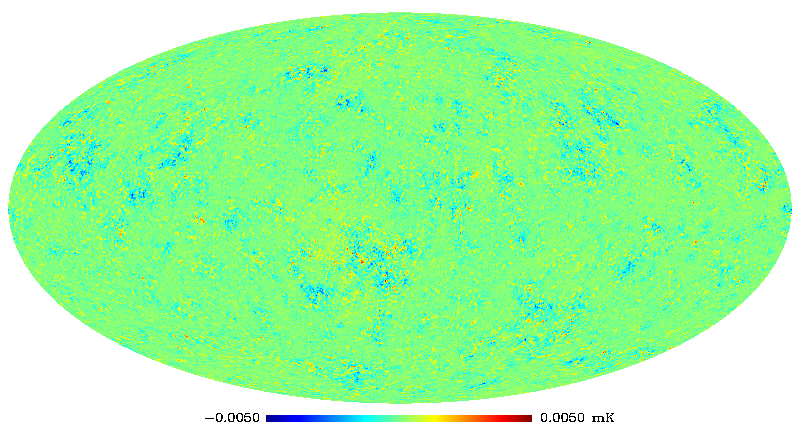
Figure 1: For illustration we show, in the upper panel, a simulated CMB map containing only a low level of local NG, namely $a_{\ell\,m}^{\mbox{\tiny upper}}=f_{\rm\,NL}\,a^{\mbox{\tiny NG}}_{\ell\,m}$ with $f_{\rm\,NL}=38$. In fact, this level of NG is so low that to emphasize it we define the temperature limits to $[-0.005,0.005]$ mK in order to make the contamination visible. In the lower panel we have a combined map made up by a Gaussian CMB map plus the upper panel non-Gaussian map, i.e., $a_{\ell\,m}^{\mbox{\tiny lower}}=a^{\mbox{\tiny G}}_{\ell\,m}+a_{\ell\,m}^{\mbox{\tiny upper}}$, with the usual scale $[-0.4,0.4]$ mK. As can be realized, there is no a visible correlation of the NG present in both maps. Statistical estimators to reveal tiny NG are required.

To analyze the potentialities of our estimator to reveal the presence of non-Gaussian signals in CMB data and to differentiate primary NG from secondary one, we produce several sets of thousands of simulated CMB maps, where one of these is a set of Gaussian CMB maps, and the other CMB maps are endowed with different amounts of primordial NG of local type. Thus, section 2 contains the details of construction and operation of our combined statistical estimator. In section 3 we apply our estimator to simulated non-Gaussian CMB maps, with several levels of contamination in different $f_{\rm\,NL}$ intervals in the range $[-10,80]$, as described throughout the text, compatible with recent Planck constraints for local NG large angles.

Afterward, we perform robustness tests by applying our estimator to simulated maps using the masks released by the Planck collaboration, and adding also realistic inhomogeneous pixel noise maps (released with the corresponding masks). In section 4, we analyze three foreground-reduced, almost full-sky, maps released by the Planck collaboration: SMICA (Spectral Matching Independent Component Analysis), NILC (Needlet Internal Linear Combination), and SEVEM (Spectral Estimation Via Expectation Maximization). Finally, we present our conclusions and final remarks in section 5.

2 The combined estimator: the Minkowski functionals and the Neural Networks tools

The new estimator proposed to identify and quantify NGs in CMB data is a combination of two statistical tools: Minkowski Functionals (hereafter MF) and Artificial Neural Networks (NN). The MFs were introduced in cosmological studies as tridimensional statistics for the analysis of the CMB and the matter distribution in the universe (see, e.g., [99, 98, 97]), Describing the morphological properties of a given field, the MFs are being used as generic estimators of NG in the 2-dimensional CMB field. The use of NNs [100] as a statistical tool for CMB studies started to being applied more recently [81, 101, 102]. Specifically, regarding Gaussian deviations in CMB data, as far as we know, there is just one reference in the literature that make use of this tool, namely [72], where the authors combine the NN with wavelet analysis in order to estimate the non-linear dimensionless parameter $f_{\rm\,NL}$ using the constraints found in WMAP-9yr CMB data.

In the next subsections we give a brief description of these tools and how we combine them to construct our estimator.

2.1 The Minkowski functionals applied to CMB maps

All the morphological properties of a $d$-dimensional space can be described using $d+1$ MFs [94]. In the case of a CMB map, a 2-dimensional temperature field defined on the sphere, $\Delta T=\Delta T(\theta,\phi)$, with zero mean and variance $\sigma^{2}$, this tool provides a test of non-Gaussian features by assessing the properties of connected regions in the map. Given a sky path ${\cal P}$ of the pixelized CMB sphere ${\cal S}^{2}$, an excursion set of amplitude $\nu_{t}$ is defined as the set of pixels in ${\cal P}$ where the temperature field exceeds the threshold $\nu_{t}$, that is, it is the set of pixels with coordinates $(\theta,\phi)\in{\cal P}$ such that $\Delta T(\theta,\phi)/\sigma\equiv\nu>\nu_{t}$.

In a two-dimensional case, for a region $R_{i}\subset{\cal S}^{2}$ with amplitude $\nu_{t}$ the partial MFs calculated just in $R_{i}$ are: $a_{i}$, the Area of the $R_{i}$ region, $l_{i}$, the Perimeter (contour length) of this Area, and $n_{i}$, the number of holes in this Area. The global MFs are obtained calculating these quantities for all the connected regions with height $\nu>\nu_{t}$. Then, the total Area $A(\nu)$, Perimeter $L(\nu)$ and Genus $G(\nu)$ are [104, 53, 103, 31]

$$A(\nu) = \frac{1}{4\pi}\int_{\Sigma}d\Omega=\sum a_{i}\,,$$ (2.1)

$$L(\nu) = \frac{1}{4\pi}\frac{1}{4}\int_{\partial\Sigma}dl=\sum l_{i}\,,$$ (2.2)

$$G(\nu) = \frac{1}{4\pi}\frac{1}{2\pi}\int_{\partial\Sigma}\kappa dl=\sum g_{i}=N_{hot}-N_{cold}\,,$$ (2.3)

where $\Sigma$ is the set of regions with $\nu>\nu_{t}$, $\partial\Sigma$ is the boundary of $\Sigma$, and, $d\Omega$ and $dl$ are the elements of solid angle and line, respectively. In the genus definition, the quantity $\kappa$ is the geodesic curvature (for more details see, e.g., [31]). This last functional can also be calculated as the difference between the number of regions with $\nu>\nu_{t}$ (number of hot spots, $N_{hot}$) and regions with $\nu<\nu_{t}$ (number of cold spots, $N_{cold}$). As defined, the MF are calculated from a given threshold $\nu_{t}$.

The MFs are currently used to test the Gaussian nature of the CMB temperature fluctuations data [104, 53, 106, 103, 105, 107, 34, 108]. As they are sensitive to weak and arbitrary non-Gaussian signals, e.g. small $f_{\rm\,NL}$ contaminations of different types, MFs are a complementary tool to optimal NG estimators based on the bispectrum calculations. Recently, the Planck Collaboration performed successful validation tests of the MF estimator with three sets of simulated CMB maps: Gaussian full-sky maps, full-sky non-Gaussian maps with noise, and non-Gaussian maps with noise and mask [93]. Afterward, they used the MFs to quantify local NG in the foreground-cleaned Planck maps [92], where some instrumental effects and known non-Gaussian contributions, like lensing, were taken into account in the analyses using realistic lensed and unlensed simulations of Planck data [93]. The constraints on local NG obtained are quite robust to Galactic residuals and are consistent to those from the bispectrum-based estimators. Moreover, these results, $f_{\rm\,NL}=38\pm 18$ for large angular scales, are basically equal to those obtained using WMAP-9yr data, that is $f_{\rm\,NL}=37.2\pm 19.9$ [93].

At this point we would like to emphasize that here we use the MFs in a different way. As shown in section 3.2.1, we use the MFs as an intermediate tool: first we apply the MFs to a CMB map to discover that the perimeter is the MF with the better capability to capture the non-Gaussian signatures that, in a second step, are efficiently recognized by the NN. In this sense, we do not use MFs to quantify NG in the map. Instead we use it just to reveal the non-Gaussian imprints present in the maps, signatures that are then systematically recognized by the trained NN.

2.2 The Neural Networks estimator

The NN are computational techniques inspired in the neural structure of intelligent organisms (animal brains), which acquires knowledge through learning [95]. A NN is composed by a large number of processing units (also called artificial neuron or nodes), configured to perform a specific action, like pattern recognition and data classification.

Aiming to emulate the behaviour of the biological brain, the simplest and most popular model for a NN for classification of patterns is the Perceptron [109, 110], consisting of a single neuron. A generalization of this model is the Multilayer Perceptron [111, 100, 95], consisting of a set of units (neurons) comprising each layer, from which the signal propagates through the NN. These NN are usually composed by an input layer, an output layer and one or more intermediate (or hidden) layers, as schematically depicted in Figure 2. The layers are interconnected through synaptic weights ($w_{ki}$) that relates the $i$-th input signal ($x_{i}$) to the $k$-th neuron, producing weighted inputs. Mathematically it is possible to represent a neuron $k$ by

$$u_{k}=\sum_{i=1}^{n}w_{ki}~{}.~{}x_{i}+b_{k},$$ (2.4)

where $n$ is the number of input signals to the $k$-th neuron. $b_{k}$ is the weighted bias input, an external parameter of the artificial neuron $k$, which can be accounted for by adding a new synapse, with input signal fixed at $x_{0}=+1$ and weight $w_{k0}=b_{k}$ [95].

The output signal of the $k$-th neuron ($y_{k}$) is generated through an activation function $\varphi_{k}$, which limits the amplitude of the output of a neuron

$$y_{k}=\varphi_{k}(u_{k})\,.$$ (2.5)

The most commonly used activation function are non-linear functions, like sigmoid and hyperbolic tangent, that can simulate more precisely the neuron behaviour in order to better emulate a real NN.

The suitable values for the weights and bias are achieved by using training (or learning) algorithms. The most popular training algorithm is the backpropagation [112], where the input signal feeds the first layer, propagating as input for the next layer, and so on until the last layer. At the end of this process a value for each neuron of the output layer, together with its corresponding error, is calculated. These values are returned to the input layer where the synaptic weights are recalculated initiating another iteration of the training process. This procedure aims to determine a suitable value for the weights of the network, and is repeated until the error value drops below a given threshold value. The architecture of the NN, like number of neurons, number of hidden layers and the specific training algorithm, can be defined according to the problem the user wants to solve. Here we used a backpropagation algorithm for the NN training with just one hidden layer, and the number of neurons was chosen according to the number of classes considered in the training: 80 neurons for 2 classes and 140 for 3 classes.

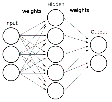
Figure 2: Multilayer Perceptron.

2.3 The classifier estimator

The combined MF+NN estimator here presented shall be termed the classifier estimator. Regarding the MFs, they were calculated using the algorithm developed by [31] and [113]. This code calculate four quantities, namely $V_{0}=A(\nu)$, $V_{1}=L(\nu)$, $V_{2}=G(\nu)$, and $V_{3}=N_{clusters}(\nu)$ the three usual MFs defined above plus an additional quantity called number of clusters, $N_{clusters}(\nu)$, for $k=3$. The latter quantity is the number of connected regions with height $\nu$ greater (or lower) than the threshold $\nu_{t}$ if it is positive (or negative), i.e., the number of hot (and cold) spots of the map.

Consider a set of $m$ simulated CMB maps. For the $i$-th simulated map, with $i=1,2,...,m$, we compute the four MFs $\{V_{k},\,k=0,1,2,3\}\equiv(V_{0},V_{1},V_{2},V_{3})$ for $n$ different thresholds $\nu=\nu_{{}_{1}},\nu_{{}_{2}},...\,\nu_{n}$, previously defined dividing the range $-\nu_{max}$ to $\nu_{max}$ in $n$ equal parts. Then, for the $i$-th map and for $k$-th MF we have not one element, but the vector

$$\,\,v_{k}^{i}\equiv(V_{k}(\nu_{{}_{1}}),V_{k}(\nu_{{}_{2}}),...V_{k}(\nu_{n}))|_{\mbox{for the $i$-th map}}\,.$$ (2.6)

In this work the values chosen for such variables are $\{\nu_{max},n\}=\{3.5,26\}$ [114, 31].

Once calculated the MFs vectors we define the training data set, $T\{x_{i},y_{i}\}$, for the NN, where $x_{i}$ is called input data and $y_{i}$ the output data, for $i=1,2,...,m$, and $m$ is the number of simulated CMB maps. This training set configuration is necessary in order to allow the network to associate a certain kind of input pattern to a specific output. We set the $i-th$ input vector as the MF vector of the $i-th$ simulated map, $x_{i}=v_{k}^{i}$, for just the $k$-th MF. The output vector, $y_{i}$, is defined according to the number of classes $N_{class}$ of the input data. For example, if we use $N$ $classes$ of maps, corresponding to ensembles with different non-Gaussian levels, we have $N_{class}=N$. Then, our $m$ output vectors have $N$ elements, $y_{i}=(1,0,...,0)$ for $class=1$, $y_{i}=(0,1,...,0)$ for $class=2$, and so on, until $y_{i}=(0,0,...,1)$ for $class=N$.

After this training process, the NN should be able to identify the same pattern in a different set of input vectors, e.g. the test data set $\{x_{j},y_{j}\}$, for $j=1,2,...,l$. That is, providing to the already trained NN a data set with $l$ input vectors $\{x_{j}=v_{k}^{j}\}$, it returns $l$ output vectors $\{y_{j}\}$ with a specified classification. It means that the NN classifies each CMB map –whose MF information is contained in $\{x_{j}\}$– according to the class it belongs, in other words, the NN classifier estimator informs its non-Gaussian level ($f_{\rm\,NL}$). After the calculation of the output vectors $\{y_{j}\}$ for a given set of simulated CMB maps, we define a way to quantify the efficiency of the NN through the counting of the number of successes (or hits) of the NN in classifying each one. We find out two ways of counting the hits of the NN:
Mode-1:  According to the limit value of 0.5 for each element of $y_{j}$ vector. In this case, e.g. for $N_{class}=N$, a vector with elements like $y_{j}=({\bf>0.5},<0.5,...,<0.5)$ indicates the $class=1$, a vector like $y_{j}=(<0.5,{\bf>0.5},...,<0.5)$ indicates $class\!=\!2$, and so on, until $y_{j}=(<0.5,<0.5,...,{\bf>0.5})$ that indicates $class=N$.
Mode-2:  Considering that the largest of the three elements of an output vector, $y_{j}$, indicate the class to which it belongs. For example, again for $N_{class}=N$, if the first element of the vector is the largest, this output vector indicates $class=1$, if the second is the largest, it indicates $class=2$, and so on, until $class=N$.
Thus, we quantify the hits of our NN by classifying each analyzed map according to its $class$, in other words according to its $f_{\rm\,NL}$ value.

3 Applying our estimator to non-Gaussian CMB maps

3.1 The Monte Carlo CMB maps

An optimal network training requires a large amount of simulated data. We produce simulated maps, termed Monte Carlo (MC) CMB maps, cut off at $\ell_{max}=500$, with $N_{\mbox{\small side}}=512$, using the HEALPix (Hierarchical Equal Area iso-Latitude Pixelization) pixelization grid [115], using the publicly available set of 1000 linear, $\{a^{\mbox{\footnotesize G}}_{\ell\,m}\}$, and 1000 non-linear (corresponding to NG of local type), $\{a^{\mbox{\footnotesize NG}}_{\ell\,m}\}$, spherical harmonics coefficients, produced by [96]. We combine them as follows

$$\,a_{\ell\,m}=a^{\mbox{\footnotesize G}}_{\ell\,m}+f_{\rm\,NL}\,a^{\mbox{\footnotesize NG}}_{\ell\,m}\,,$$ (3.1)

and normalize the maps using a power spectrum generated by the CAMB online tool using the Planck concordance cosmological model [6].

To test the efficiency of our estimator we use MC CMB maps containing the degree of contamination defined by the recent constraints found by Planck [93], that is, $f_{\rm\,NL}=38\,\pm\,18$ at 68.3% confidence level. For this, we test our estimator with sets of MCs endowed with levels of contamination in the ranges: $f_{\rm\,NL}\,=\,[-10,10],[10,30],\,[28,48],[30,50],[40,60],\,[60,80]$, in order to have normal distributions with mean 0, 20, 38, 40, 50 and 70, respectively.

3.2 Quantitative analysis of NG in CMB maps

3.2.1 Preliminary tests: sensitivity of the classifier estimator

We begin the tests using just two $classes$, corresponding to MC CMB maps constructed using $f_{\rm\,NL}=[-10,10]$ ($class=1$) and $f_{\rm\,NL}=[40,60]$ ($class=2$). We started using $m=1000$ Area vectors ($v_{0}^{i}$, for $i$ = 1, …, 1000) for training the NN, 500 of each class. The output vectors were defined as, $y_{i}=(1,0)$ for $class=1$ and $y_{i}=(0,1)$ for $class=2$. After trained, the NN was applied to a test data set, of the same size as the training one, $l=m=1000$ Area vectors, with again 500 of each class. This procedure of training and test of NNs was repeated for each one of the three other kinds of MFs ($k=1,2$, and $3$).

Analyzing the output returned by the NN when applied to test data set, for each sort of MF, we had the results summarized in Table 1. The last two columns are the NN Hits, indicating the percentage of correct indication (right pattern recognition) according to both Modes 1 and 2, and the corresponding Mean Square Error (MSE), that measure the NN’s performance comparing the returned values ($y_{j}^{ret}$) to those expected ($y_{j}^{exp}$), defined as

$$MSE=\frac{1}{l}\sum_{j=1}^{l}(y_{j}^{exp}-y_{j}^{ret})^{2}\,,$$ (3.2)

for $j=1,2,...,l$, where $l$ is the number of MF vectors in the test data set. These preliminary tests allow the comparison of sensitivities for each MF when used together with the NN classifier estimator. From these results it is possible to infer that the sensitivity of MFs, from the best to worst, is $\mbox{Perimeter}\,\gtrsim\,\mbox{Genus}\,\gtrsim\,N_{clusters}\,\gg\,\mbox{Area}$, very similar to what was obtained by [31].

Using $m=2000$ MF vectors to train our NN, each set of $1000$ corresponding to the same classes 1 and 2, it was possible to check their sensitivity when increasing the size of the training data set. The results, also presented in Table 1, show a small improvement relatively to the test using only $1000$ MF input vectors. In the next subsection we show the results from a second test, making clear how this feature improves the accuracy of our results.

Table 1: Results of the sensitivity tests.

f${}_{\mbox{\sc\footnotesize nl}}$	m	l	$N_{class}$	MF	Hits - Mode-1/Mode-2 a (%)	MSE b
				Area	59.4 / 63.7	0.240
[-10,10], [40,60]	1000	1000	2	Perimeter	85.5 / 87.1	0.106
				Genus	78.5 / 81.0	0.146
				$N_{clusters}$	74.5 / 81.5	0.146
				Area	62.7 / 64.5	0.226
[-10,10], [40,60]	2000	1000	2	Perimeter	96.4 / 96.5	0.049
				Genus	96.7 / 96.9	0.049
				$N_{clusters}$	95.7 / 95.9	0.062
aThe two ways to calculate the hits of NN (see sect. 2.3). bMean Square Error (see text for details).

3.2.2 Testing the estimator with lower non-Gaussian contamination level and greater number of classes

We find out that the minimal separation between two neighbor $classes$, in order to guarantee a successful classification of $\sim 95\%$ of tested maps, is $\Delta f_{NL}\sim 35$ which gives the 2-$\sigma$ error of our method.

As recently obtained from Planck data, the current limit for the non-linear parameter is $f_{\rm\,NL}=38\pm 18$, at 68% confidence level. Our specific aim here is to test an estimator sensitive enough to identify the presence of weak levels of NG within this constraint. Therefore, taking into account the error of our method and the Planck constraint, we shall test our classifier estimator using three classes, $N_{class}=3$, of simulated maps: one of nearly Gaussian CMB maps, $f_{\rm\,NL}=[-10,10]$ ($class=1$, $\langle f_{\rm\,NL}\rangle=0$), and the other made with two different levels of local NG: with $f_{\rm\,NL}=[28,48]$ ($class=2$, $\langle f_{\rm\,NL}\rangle=38$) and $f_{\rm\,NL}=[60,80]$ ($class=3$, $\langle f_{\rm\,NL}\rangle=70$), all three ensembles having the variance equal to 7.5.

According to our results obtained in the last sub-section the size of the training set appears to be a determinant factor in obtaining a good classifier, besides the fact that, between the four MFs, the Perimeter appears to be the most sensitive to reveal the non-Gaussian signal. Then, we started applying our estimator in $m=3000$ Perimeter vectors, $l=1000$ of each class. The same was repeated for $m=4500$, $6000$, $7500$, $9000$, $10500$, $12000$, $13500$, $15000$, $16500$, $18000$ and $19500$, $m/3$ vectors of each class. For all applications we carried out, it was used a set of $l/3=500$ input Perimeter vectors in order to test the trained NN.

Figure 3 shows the average number of hits resulting of each NN training, considering the two ways to count it, that is, Mode-1 and Mode-2. With this graph it is possible to verify that the larger the training data set the better trained will be the NN and more precise the classification. However, we can also identify a point ($m/3\sim 4500$) where the hits do not improve significantly even further increasing the training set. Hence, we stopped our test with $m=19500$, with an average hits of 99.6%, according Mode-1, and 99.9%, according to Mode-2. The hits for each one of the classes 1, 2, and 3 are, respectively: 99.6%, 99.8% and 99.6%, according to Mode-1, and 100%, 99.8% and 100%, according to Mode-2.

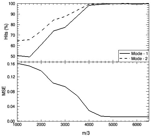
Figure 3: Average Hits (above) and Mean Square Error (bellow) in estimating the $f_{\rm\,NL}$ range using a NN previously trained with $m$ Perimeter vectors (Gaussian and non-Gaussian MC CMB maps).

3.3 Robustness analyses using Planck data

3.3.1 Additional products from foreground-cleaned Planck maps

The major challenge in making foreground-reduced CMB maps is to clearly understand all the possible sources of contaminations contributing to the set of different frequency maps observed in a given CMB survey. This is necessary to estimate their effects on the data in order to subtract the foreground components from the raw maps and to leave the largest possible amount of primordial cosmological signal. The Planck collaboration uses the suitable framework for this task, that is, the component separation technique [92], which aims to identify the sources of contaminating emissions that contribute dissimilarly to the set of nine frequency bands, from 30 to 857 GHz, observed by Planck [6]. In fact, four distinct component separation algorithms [92] were employed by the Planck collaboration to identify and remove the signal coming from the various contaminants. At large angles, galactic foregrounds are dominant, including diffuse emission (synchrotron, bremsstrahlung, thermal dust, and anomalous microwave emission) and line emission from carbon monoxide. On the other hand, extragalactic foregrounds dominate at small scales and can be classified into two categories: discrete detectable compact sources and the collective signal from unresolved sources (mainly radio and infrared galaxies, but also from clusters of galaxies via the Sunyaev-Zel’dovich effect). It is worth noticing that the Planck team just masked the bright cosmic objects to eliminate extragalactic foregrounds.

As a result, the Planck collaboration has released three high resolution, almost full-sky foreground-cleaned CMB maps  [92], termed SMICA (Spectral Matching Independent Component Analysis) [116], NILC (Needlet Internal Linear Combination) [89], and SEVEM (Spectral Estimation Via Expectation Maximization) [117]. These high resolution maps have $N_{side}=2\,048$ and effective beam fwhm$=5$ arcmin. The performance of the foreground-cleaning algorithms has been carefully investigated with simulated maps. In particular, each component separation algorithm processes differently the multi-contaminated sky regions obtaining, as a consequence, different final foreground-cleaned regions for each procedure. These regions are defined by the so-called Component Separation Confidence masks (briefly termed CS-masks), which have $f_{sky}=0.89,0.93,0.76$, for the SMICA, NILC, and SEVEM maps, respectively. Each CMB map was released with its own CS-mask, outside which the corresponding CMB signal is considered statistically robust. Regarding the masks, it is worth mentioning that the Planck team produced the U73 mask, which is the union of the above mentioned masks, it is more restrictive since it has $f_{sky}=0.73$ and is used for evaluation purposes [92]. In addition, the mapmaking of these foreground-cleaned maps produced an estimative of the noise (mainly due to the non-uniform strategy for scanning the CMB sky) in each pixel’s map, information that was also released jointly to its corresponding CMB map.

The availability of these CS-masks and pixel noise maps allows to test the NG statistical estimators in non ideal situations, aiming to mimic some Planck data features. This is done analyzing simulated maps which include both effects: masks and noise, in addition to local NG. Nevertheless, this is a partial approach, because other contaminating contents, which are not taken into account in the simulations, could be present in the data. The consequences of this ignorance about unknown NGs in data maps will be discussed below.

3.3.2 Noise contamination and mask influence to the classifier estimator

The aim of the following tests is to verify the performance of our estimator in more realistic situations, using for this different masks and realistic inhomogeneous pixel noise released by Planck. Moreover, in all these tests we take into account the Planck effective beam, fwhm$=5$ arcmin, in the construction of the MC CMB maps.

Since the previous tests (Figure 3) showed that for $m/3>4500$ Perimeter-MF vectors the number of hits do not improve significantly, we decided to perform all the next tests using $m/3=5000$ MC CMB maps. For the tests of all the following trained NN it was used $l/3=500$ Perimeter-MF vectors.

We divide the analyses in two steps: the first one serves to verify the impact of using masks, with different $f_{sky}$ factors, and the other one to check the estimator performance when the maps are contaminated by inhomogeneous noise, beside using masks.

1. Sky cuts: the Planck masks

The firsts robustness tests of the NN classifier estimator consists on the analysis of MC CMB maps with two sky cuts, given by two masks released by Planck Satellite: 1) the CS-mask of the SMICA map, hereafter called SMICA-mask; and 2) the U73 mask. Therefore, the test of the masks were performed applying the estimator to two sets of maps, each one composed by a different sky fraction. Both tests used three classes of maps, composed by a non-Gaussian signal such as $f_{\rm\,NL}=[-10,10]$ ($class=1$), $[28,48]$ ($class=2$) and $[60,80]$ ($class=3$). The average hits resulting from these tests, that is the rate of successfully detection cases, are shown in Table 2.

Comparing the values presented in the second and third columns of Table 2 with the values of Table 1 we conclude that the use of masks does not influence the efficiency of the NN classifier estimator, and the average hits remains larger than 99%.

2. Inhomogeneous noise and masks

A second set of robustness analyses consists on the application of our estimator to MC CMB maps contaminated with real non-Gaussian inhomogeneous noise from Planck data. In order to exhaustively test our combined estimator, various combinations of noise maps and different masks were applied to the MC CMB maps before calculating the input Perimeter vectors. These pixel noise maps are those corresponding to the SMICA, NILC, and SEVEM Planck maps, and the masks are the same used in the previous tests. Again it was used three classes of synthetic maps, constructed using the same ranges of $f_{\rm\,NL}$ values used in previous analysis, that are: $f_{\rm\,NL}=[-10,10]$, $[28,48]$ and $[60,80]$. Then, it was performed a total of four tests of the estimator, in four different sets of synthetic maps, that are: two sets of maps contaminated by SMICA noise, using 1) the U73 mask and 2) their own CS-mask, to analyze the influence of the two kinds of masks in the presence of the same noise, and two sets of maps contaminated with 3) SEVEM and 4) NILC noises, but using the same mask, U73, testing the impact of these two kinds of noise even with a rigorous sky cut.

In addition, we still tested the efficiency of our estimator when applied to MC CMB maps whose primordial non-Gaussian signal corresponds to contiguous $f_{\rm\,NL}$ ranges, namely, $[-10,10]$, $[10,30]$ and $[30,50]$. This test was carried out just in the case of using the SMICA noise as contaminant and the U73 mask.

The hits numbers for each test, as well as the corresponding MSE values, are presented in Table 2. Again, there is no impact in using different masks, but the inclusion of inhomogeneous noise makes the number of hits become slightly lower. These results allow us to conclude that our combined estimator is, basically, equally efficient in both situations analyzed, namely applying a mask but not noise and using a mask plus a pixel noise map.

The last point to discuss are the results obtained in Table 2 when using input maps endowed with primordial non-Gaussian signal in contiguous ranges of $f_{\rm\,NL}$ values, namely $[-10,10]$, $[10,30]$ and $[30,50]$. In this case the hit’s numbers are even lower, with higher MSE value. This fact evidences the difficulty of the NN to identify non-Gaussian patterns when trained with sets of MCs having contaminations whose intensities $f_{\rm\,NL}$ belong to three adjacent intervals.

Table 2: Results of the robustness analysis.

$f_{\rm\,NL}{{}^{a}}$	NN reference	MC CMB map	Hitsb (%)	MSE
	NNnc-1	noiseless + SMICA-mask	99.4 / 99.7	0.01
	NNnc-2	noiseless + U73	99.6 / 99.7	0.01
$[-10,10],[28,48],[60,80]$	NNnc-3	SMICA noise + SMICA-mask	98.4 / 99.1	0.03
	NNnc-4	SMICA noise + U73	97.3 / 98.5	0.02
	NNnc-5	SEVEM noise + U73	98.1 / 98.9	0.03
	NNnc-6	NILC noise + U73	98.6 / 99.3	0.03
$[-10,10],[10,30],[30,50]$	NNc-7	SMICA noise + U73	96.5 / 97.2	0.05
a Contiguous ($c$) and not contiguous (${nc}$) intervals of the parameter $f_{\rm\,NL}$ in the MC simulations. b Hits corresponding to Mode-1/Mode-2.

4 Analysis of Planck CMB maps

The purpose, and natural consequence, of the development of a new statistical tool, after exhaustive tests in synthetic data, is its application to real data. As discussed before, the robustness tests presented here were done using Planck data, like real pixel noise maps and cut-sky masks, because our aim is to know the impact of these effects on our estimator for a posterior application of our trained NN to corresponding CMB data. For each foreground-cleaned Planck CMB map we used the suitably trained NN, that is, that one trained using MCs CMB maps to which we added pixel noise contamination and to which we apply a sky-cut mask. Thus, the analysis of the three Planck CMB maps were performed according to the following correspondence:

$$\mbox{NN}^{nc}\mbox{-3} \Longrightarrow$$ SMICA map + SMICA-mask (4.1)

$$\mbox{NN}^{nc}\mbox{-4} \Longrightarrow$$ SMICA map + U73 (4.2)

$$\mbox{NN}^{nc}\mbox{-5} \Longrightarrow$$ NILC map + U73 (4.3)

$$\mbox{NN}^{nc}\mbox{-6} \Longrightarrow$$ SEVEM map + U73 (4.4)

$$\mbox{NN}^{c}\mbox{-7}\,\,\, \Longrightarrow$$ SMICA map + U73 (4.5)

where the indices 3-7 indicate the trained-NN used in each case (according to the input maps used for each one), and $c$ ($nc$) refers to the contiguous (not contiguous) intervals employed in the analyses, as specified in Table 2.

As discussed before, the expected output of a NN is a vector whose elements are $\cal{O}$(0) or $\cal{O}$(1), where $\cal{O}$(0) ($\cal{O}$(1)) means that the numerical value is very near to zero (to one). That is, in our case, using $N_{class}=3$, $y_{\mbox{\tiny Planck map}}=$ ($\cal{O}$(1), $\cal{O}$(0), $\cal{O}$(0)), or $y_{\mbox{\tiny Planck map}}=$ ($\cal{O}$(0), $\cal{O}$(1), $\cal{O}$(0)), or $y_{\mbox{\tiny Planck map}}=$ ($\cal{O}$(0), $\cal{O}$(0), $\cal{O}$(1)), indicating the class of a given map. However, the NN returned $y$ vectors with elements different from those expected, presenting values of order $\cal{O}$(10), or even higher. These kind of discrepancy occurs when using training and test data sets with very different characteristics. Then the NN response is totally comprehensive when comparing a Perimeter vector from Planck CMB map to that ones obtained from the MC CMB maps, which are visually different, as shown in Figure 4.

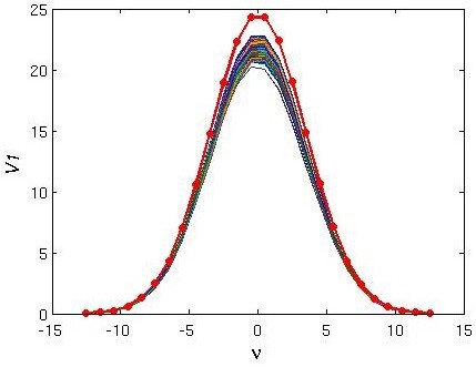
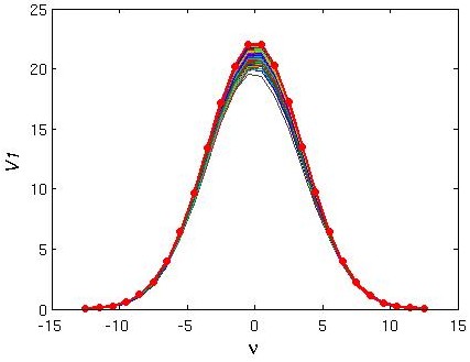
Figure 4: Plot of the Perimeter-MF calculated from the MC CMB maps (multicoloured lines) and from SMICA Planck map (red thick line). Left: Perimeter vectors calculated from the original maps after applying the U73 mask. Right: The same as in the left, but all the maps is smoothed with fwhm$=3$ arcmin before calculate the Perimeter.

It is worth to emphasize that the MFs are sensitive to the resolution scale of the temperature map in analysis [118]. In this sense, a possible explanation for the difference in the Perimeter’s amplitudes observed between synthetic and Planck maps (left panel of Figure 4) is that, even performing MC simulations using the Planck effective beam of fwhm$=5$ arc-min, the smoothing scales of these maps are still not fully compatible. Aware of this problem, and attempting to solve it, we analyze the effect of using a smoothing tool in all the MC CMB maps (training and test data sets), as well as in the Planck maps, before the calculation of the MFs. It was verified that this procedure makes the characteristics of these maps a bit more consistent, obtaining more compatibles Perimeter’s vectors (right panel of Figure 4). The Gaussian beam used for smoothing all the maps was fwhm$=3$ arcmin. This value was chosen as a compromise: it is large enough in such a way that synthetic and real maps became more consistent, and it is small enough to not decrease the amplitude of the non-Gaussian signal, under the condition that does not modify the angular power spectrum of the maps. It is worth to point out that this procedure does not influence the results of applying the NN to the test data set, still obtaining hits numbers as those presented in Table 2 for all the cases. Moreover, when applying the NN, trained using Perimeter vectors from these slightly smoothed maps, to those obtained from the smoothed Planck CMB maps, we verify a significant improvement of the output vectors. Following the same correspondences in 4.1-4.5, the vectors obtained were, respectively:

$$y_{\tiny\mbox{NN}^{nc}\mbox{-3}} = (-0.45,0.99,0.46)$$ (4.6)

$$y_{\tiny\mbox{NN}^{nc}\mbox{-4}} = (-0.11,0.75,0.35)$$ (4.7)

$$y_{\tiny\mbox{NN}^{nc}\mbox{-5}} = (-0.25,1.97,-0.72)$$ (4.8)

$$y_{\tiny\mbox{NN}^{nc}\mbox{-6}} = (-0.37,-3.61,4.98)$$ (4.9)

$$y_{\tiny\mbox{NN}^{c}\mbox{-7}}\,\; = (0.55,-2.11,2.56)$$ (4.10)

As observed, there is an improvement in the consistency of the output vectors $y$, but it is not enough to give us a reliable result because the elements are still quite different from those expected.

We interpret these results in the sense that, under these circumstances, the NN is not able to recognize the full pattern of NG appearing in the Planck maps. These circumstances means that even including noise, using masks and running a smoothing procedure, in such a way to let the MC CMB maps more similar to Planck CMB maps, the synthetic maps will not mimic them well enough, since we do not have a total knowledge about the full contents of these maps. Moreover, and complementing this idea, the imprecision of the NN could be indicating that the NGs present in the Planck maps are not only of local type. In this case, since the simulated data do not have contributions apart from the local non-Gaussianity, the estimator shows that the synthetic and Planck non-Gaussianities contents are, indeed, different.

Nevertheless, even when the results from the application of our NNs into Planck CMB maps reveal certain imprecision of the NN, one can still verify that the output vectors indicate a level of non-Gaussian contamination that agree with the recent results obtained with WMAP-9yr and Planck data. Analysing these output vectors in the sense that its higher element denote the class of the corresponding map (as in Mode-2), that is, the range of $f_{\rm\,NL}$ values that the NN indicates for the non-Gaussian contamination, we get the ranges: $f_{\rm\,NL}=[28,48]$ for the output vectors of relations (4.6) to (4.9), and $[30,50]$ for the output vector of the relation (4.10). It is worth mentioning that in some approaches it is not possible to exhibit the results in the form: average value (or most probable value) $\pm$ one standard deviation, i.e., $\overline{\mbox{X}}\pm\Delta\mbox{X}$. In such a case, alternative ways are employed to measure the efficiency of a method (as e.g. in [45, 46, 44, 34]). For this reason, here we use the MSE value, which is the standard criterion often used to measure the performance of a NN (as well as RMSE, the squared root of MSE), and, therefore, an appropriate error measurement to evaluate our estimator (see, e.g., [100, 121, 120, 119]).

5 Conclusions

The standard inflationary model predicts a Gaussian distribution of CMB anisotropy, while other theories predict the existence of deviations from the initial Gaussian condition. The detection, or not, of non-Gaussian (NG) signatures on CMB data can help to exclude many inflationary models and discriminate between different mechanisms for generating cosmological perturbations. Therefore, the search for non-Gaussian signals in new CMB data sets has become the target of several working groups, analyzing so far mainly the WMAP data [28, 41, 32, 33, 40, 48, 37, 39, 42, 45, 46, 47, 43, 44, 38, 49, 88]. Currently, with the recent release of Planck data, analyses following different approaches are being done to confirm independently the constraints on primordial NG found by the Planck team, taking into account that many estimators are needed to identify diverse types of NG, their intensities, and corresponding angular scales dependences [93, 26, 31, 34, 44].

We presented here an estimator developed to improve the determination of constraints on the primordial NG, gathering a tool already widely used to study non-Gaussian signal, the Minkowski Functionals, and another one complementary and very new in this context, the Artificial Neural Networks. The joint use of these tools provide a classifier estimator which performs a comparison analysis, as described throughout the text. The estimator was applied to a large amount of MC CMB simulations divided in classes according to the non-Gaussian level of contamination, that is, the $f_{\rm\,NL}$ value. One conclusion was that the higher the number of maps (MF vectors) used as input the better the performance of the estimator, but with a limit in which the results stop to improve (Figure 3). We also tested the joint use of each of the four kinds of MF with the NN, and from the results of each case it was possible to verify that the Perimeter-MF is the most sensitive to non-Gaussian signal, providing a pattern more easily recognized by the NN (see Table 1).

A large number of tests were performed in order to evaluated the performance of the estimator in different configurations, and to verify what can influence the results. We notice that the use of masks have no impact, and the inclusion of inhomogeneous noise does not affect significantly as well. Moreover, the performance of the estimator can be influenced by the number of classes and the degree of NG. When using just two classes, corresponding to MC CMB maps constructed using $f_{\rm\,NL}$ values more widely spaced, it is not necessary to use a very large number of neurons, whereas using three classes require a larger number of them in order to train the NN.

As a matter of fact, the capability to recognize primary and secondary CMB NGs, besides having a good performance in capturing weak NG contaminations in the data are essential features in a statistical estimator. For this, we analyzed the capacity of our combined estimator to distinguish between primary and secondary NGs. Training the Neural Network with two sets, one of nearly Gaussian CMB maps ($|f_{\rm\,NL}|\leq 10$) endowed with realistic inhomogeneous Planck noise (i.e., secondary non-Gaussianity) and the other of CMB maps with weak primordial NG ($28\leq f_{\rm\,NL}\leq 48$), we then test an ensemble composed of CMB maps with contaminations of one of these types: half of them have primordial NG and the other half have secondary non-Gaussian contaminations. The results show that our method successfully classifies $\sim 95\%$ of the tested maps as being Gaussian plus inhomogeneous noise CMB maps or CMB maps with primordial NG.

All these tests show that the method is very efficient when applied to data similar to which the NN was trained on. The best performance shown by our estimator occurs when the type of NG present in the data is known, so that the training of the NN with MCs contaminated with such NG is effective. This means that, when applied to data containing non-Gaussian components with which the NN have been not trained the estimator become imprecise. A similar situation was recently verified by [34], who pointed out that simulated CMB maps, on large angular scales, with diverse levels of NG of local type cannot reproduce the anomalous outcomes found in the ILC-7yr full-sky WMAP map. Nevertheless, the results of our analyses of the foreground-cleaned Planck maps are in good agreement with last constraints, for large angular scales, from WMAP-9yr and Planck data analyses, i.e., $f_{\rm\,NL}=38\pm 18$ [93]. Summarizing, our conclusions point to the following approach: by considering a given type of contamination in the training data set, here the local NG, the NN recognizes satisfactorily $\gtrsim$ 98% of the examined maps. This means that, adding contributions of other non-Gaussian types to simulated maps, in order to suitable instruct the NN’s training data set, would let to an improved analysis of a CMB map. In this context, our results show that this estimator can be considered a useful tool to detect and constrain primordial, as well as secondary, non-Gaussian effects possibly present in CMB data.

References

- [1] C. L. Bennett, M. Halpern and G. Hinshaw, First Year Wilkinson Microwave Anisotropy Probe (WMAP) Observations: Preliminary Maps and Basic Results, ApJS 148 (2003) 1 [astro-ph/0302207]
- [2] G. Hinshaw et al., Three-Year Wilkinson Microwave Anisotropy Probe (WMAP) Observations: Temperature Analysis, ApJS 170 (2007) 288 [astro-ph/0603451]
- [3] G. Hinshaw et al., Five-Year Wilkinson Microwave Anisotropy Probe Observations: Data Processing, Sky Maps, and Basic Results, ApJS 180 (2009) 225 [arXiv:0803.0732]
- [4] D. Larson et al., Seven-Year Wilkinson Microwave Anisotropy Probe (WMAP) Observations: Power Spectra and WMAP-Derived Parameters, ApJS 192 (2011) 16 [arXiv:1001.4635]
- [5] C. L. Bennett et al., Nine-Year Wilkinson Microwave Anisotropy Probe (WMAP) Observations: Final Maps and Results, arXiv:1212.5225
- [6] Planck Collaboration, Planck 2013 results. I. Overview of products and scientific results, arXiv:1303.5062
- [7] Planck Collaboration, Planck Collaboration XV. 2013, "CMB power spectra and likelihood, arXiv:1303.5075
- [8] M. Colless et al., The 2dF Galaxy Redshift Survey: spectra and redshifts, MNRAS 328 (2001) 1039 [astro-ph/0106498]
- [9] D. H. Jones et al., The 6dF Galaxy Survey: samples, observational techniques and the first data release, MNRAS 355 (2004) 747 [astro-ph/0403501]
- [10] M. F. Skrutskie et al., The Two Micron All Sky Survey (2MASS), AJ 131 (2006) 1163
- [11] M. A. Strauss et al., Spectroscopic Target Selection in the Sloan Digital Sky Survey: The Main Galaxy Sample, AJ 124 (2002) 1810 [astro-ph/0206225]
- [12] N. Bartolo, S. Matarrese and A. Riotto, Non-Gaussianity and the Cosmic Microwave Background Anisotropies, Advances in Astronomy (2010) 157079 [arXiv:1001.3957]
- [13] N. Bartolo et al., Second-order matter perturbations in a LambdaCDM cosmology and non-Gaussianity, Class. Quant. Grav. 27 (2010) 124009 [arXiv:1002.3759]
- [14] E. Komatsu et al., Non-Gaussianity as a Probe of the Physics of the Primordial Universe and the Astrophysics of the Low Redshift Universe, arXiv:0902.4759
- [15] L. R. Abramo, A. Bernui and T. S. Pereira, Searching for planar signatures in WMAP, JCAP 12 (2009) 013
- [16] L. R. Abramo and T. S. Pereira, Testing gaussianity, homogeneity and isotropy with the cosmic microwave background, Advances in Astronomy (2010) 378203 [arXiv:1002.3173]
- [17] A. P. A. Andrade, C. A. Wuensche and A. L. B. Ribeiro, Predictions of Mixed Non-Gaussian Cosmological Density Fields for the Cosmic Microwave Background Radiation, ApJ 602 (2004) 555 [astro-ph/0312028]
- [18] X. Chen, Primordial Non-Gaussianities from Inflation Models, Advances in Astronomy (2010) 638979 [arXiv:1002.1416]
- [19] A. Golovnev, Non-Gaussian Probability Distribution of the CMB Angular Power Spectra, in Cosmic Structure and Evolution, arXiv:0910.5280
- [20] M. Kawasaki, K. Nakayama and F. Takahashi, Hilltop non-gaussianity, JCAP 01 (2009a) 026 [arXiv:0810.1585]
- [21] M. Kawasaki, K. Nakayama, T. Sekiguchi, T. Suyama and F. Takahashi, A general analysis of non-gaussianity from isocurvature perturbations, JCAP 01 (2009b) 042 [arXiv:0810.0208]
- [22] E. Komatsu, Hunting for primordial non-Gaussianity in the cosmic microwave background, CQG 27 (2010) 124010 [arXiv:1003.6097]
- [23] D. Pogosyan, C. Pichon and C. Gay, Non-Gaussian extrema counts for CMB maps, Phys. Rev. D 84 (2011) 083510 [arXiv:1107.1863]
- [24] M. Sasaki and D. Wands, Non-linear and non-Gaussian cosmological perturbations, Class. Quant. Grav. 27 (2010) 120301
- [25] C. A. Valenzuela-Toledo and Y. Rodríguez, Non-gaussianity from the trispectrum and vector field perturbations, Phys. Lett. B 685 (2010) 120 [arXiv:0910.4208]
- [26] E. Komatsu, The Pursuit of Non-Gaussian fluctuations in the Cosmic Microwave Background, arXiv:astro-ph/0206039
- [27] N. Bartolo, E. Komatsu, S. Matarrese and A. Riotto, Non-Gaussianity from inflation: Theory and observations, Phys. Rep. 402 (2004) 103 [astro-ph/0406398]
- [28] E. Komatsu, Wilkinson Microwave Anisotropy Probe constraints on non-Gaussianity, New Astronomy Reviews 47 (2003b) 797
- [29] D. Babich, Optimal estimation of non-Gaussianity, Phys. Rev. D 72 (2005) 043003 [astro-ph/0503375]
- [30] M. Liguori et al., Primordial non-Gaussianity and Bispectrum Measurements in the Cosmic Microwave Background and Large-Scale Structure, Advances in Astronomy (2010) 980523 [arXiv:1001.4707]
- [31] A. Ducout, F. Bouchet, S. Colombi, D. Pogosyan and S. Prunet, Non Gaussianity and Minkowski Functionals: forecasts for Planck, arXiv:1209.1223
- [32] L.-Y. Chiang, P. D. Naselsky, O. V. Verkhodanov and M. J. Way, Non-Gaussianity of the Derived Maps from the First-Year Wilkinson Microwave Anisotropy Probe Data, ApJ 590 (2003) L65 [astro-ph/0303643]
- [33] L.-Y. Chiang, P. D. Naselsky and P. Coles, Departure from Gaussianity of the Cosmic Microwave Background Temperature Anisotropies in the Three-Year WMAP Data, ApJ 664 (2007) 8 [astro-ph/0603662]
- [34] H. I. Modest et al., Scale-dependent non-Gaussianities in the CMB data identified with Minkowski functionals and scaling indices, MNRAS 428 (2013) 551
- [35] A. Bernui, C. Tsallis and T. Villela, Temperature Fluctuations of the Cosmic Microwave Background Radiation: A Case of Nonextensivity?, Phys. Lett. A 356 (2006) 426 [astro-ph/0512267]
- [36] A. Bernui, C. Tsallis and T. Villela, Deviation from Gaussianity in the cosmic microwave background temperature fluctuations, Europhys. Lett. 78 (2007) 19001 [astro-ph/0703708]
- [37] A. Bernui, Is the cold spot responsible for the CMB North-South asymmetry?, Phys. Rev. D 80 (2009) 123010 [arXiv:0912.1147]
- [38] P. Bielewicz, B. D. Wandelt and A. J. Banday, A search for concentric rings with unusual variance in the 7-year WMAP temperature maps using a fast convolution approach, arXiv:1207.6905
- [39] M. Cruz, E. Martínez-González and P. Vielva, The WMAP cold spot, arXiv:0901.1986
- [40] J. D. McEwen et al., A high-significance detection of non-Gaussianity in the WMAP 5-year data using directional spherical wavelets, MNRAS 388 (2008) 659 [arXiv:0803.2157]
- [41] C.-G. Park, Non-Gaussian signatures in the temperature fluctuation observed by the Wilkinson Microwave Anisotropy Probe, MNRAS 349 (2004) 313 [astro-ph/0307469]
- [42] D. Pietrobon, P. Cabella, A. Balbi, G. de Gasperis and N. Vittorio, Constraints on primordial non-Gaussianity from a needlet analysis of the WMAP-5 data, MNRAS 396 (2009) 1682 [arXiv:0812.2478]
- [43] D. Pietrobon et al., Needatool: A Needlet Analysis Tool for Cosmological Data Processing, ApJ 723 (2010) 1 [arXiv:1010.1371]
- [44] C. Räth , A. J. Banday, G. Rossmanith, H. Modest, R. Sütterlin, K. M. Górski, J. Delabrouille and G. E. Morfill, Scale-dependent non-Gaussianities in the WMAP data as identified by using surrogates and scaling indices, MNRAS 415 (2011) 2205 [arXiv:1012.2985]
- [45] G. Rossi, R. K. Sheth, C. Park and C. Hernández-Monteagudo, Non-Gaussian distribution and clustering of hot and cold pixels in the five-year WMAP sky, MNRAS 399 (2009) 304 [arXiv:0906.2190]
- [46] G. Rossmanith, C. Räth, A. J. Banday and G. Morfill, Non-Gaussian Signatures in the five-year WMAP data as identified with isotropic scaling indices, MNRAS 399 (2009) 1921 [arXiv:0905.2854]
- [47] P. Vielva and J. L. Sanz, Analysis of non-Gaussian CMB maps based on the N-pdf. Application to WMAP data, MNRAS 397 (2009) 837 [arXiv:0812.1756]
- [48] Y. Wiaux, P. Vielva, R. B. Barreiro, E. Martínez-González and P. Vandergheynst, Non-Gaussianity analysis on local morphological measures of WMAP data, MNRAS 385 (2008) 939 [arXiv:0706.2346]
- [49] A. Gruppuso, P. Natoli, F. Paci, F. Finelli, D. Molinari, A. De Rosa and N. Mandolesi, Low variance at large scales of WMAP 9 year data, JCAP 07 (2013) 047 [arXiv:1304.5493]
- [50] G. Hinshaw et al., Nine-Year Wilkinson Microwave Anisotropy Probe (WMAP) Observations: Cosmological Parameter Results, arXiv:1212.5226
- [51] N. Bartolo, S. Matarrese and A. Riotto, Non-Gaussianity in the cosmic microwave background anisotropies at recombination in the squeezed limit, JCAP 02 (2012) 017 [arXiv:1109.2043]
- [52] S. Chongchitnan and J. Silk, Primordial Non-Gaussianity and Extreme-Value Statistics of Galaxy Clusters, Phys. Rev. D 85 (2012) 063508 [arXiv:1107.5617]
- [53] E. Komatsu et al., WMAP first-year data: Non-Gaussianity, ApJS 148 (2003a) 119
- [54] Y. Takeuchi, K. Ichiki and T. Matsubara, Application of cross correlations between CMB and large scale structure to constraints on the primordial non-Gaussianity, Phys. Rev. D 85 (2012) 043518 [arXiv:1111.6835]
- [55] L. Verde, L. Wang, A. F. Heavens and M. Kamionkowski, Large-Scale structure, the cosmic microwave background and primordial non-Gaussianity, MNRAS 313 (2000) 141
- [56] J.-Q. Xia, C. Baccigalupi, S. Matarrese, L. Verde and M. Viel, Constraints on Primordial Non-Gaussianity from Large Scale Structure Probes., JCAP 08 (2011) 033 [arXiv:1104.5015]
- [57] A. P. S. Yadav and B. D. Wandelt, Primordial Non-Gaussianity in the Cosmic Microwave Background, Advances in Astronomy (2010) 565248 [arXiv:1006.0275 ]
- [58] N. Aghanim and O. Forni, Non-Gaussian signature induced by the SZ effect of galaxy clusters, arXiv:astro-ph/0003256
- [59] N. Aghanim, S. Majumdar and J. Silk, Secondary anisotropies of the CMB, Rept. Prog. Phys. 71 (2008) 066902 [arXiv:0711.0518]
- [60] P. K. Aluri et al., Effect of Foregrounds on the CMBR Multipole Alignment, MNRAS 414 (2011) 1032 [arXiv:1007.1827]
- [61] P. K. Aluri, P. K. Räth and P. Jain, Pixel and multipole space correlation analysis of CMB with foregrounds, arXiv:1202.2678
- [62] A. Cooray, Non-Gaussian aspects of thermal and kinetic Sunyaev-Zel’dovich effects, Phys. Rev. D 64 (2001) 063514 [astro-ph/0105063]
- [63] M. Cruz et al., Anomalous variance in the WMAP data and Galactic Foreground residuals, MNRAS 412 (2011) 2383 [arXiv:1005.1264]
- [64] D. Munshi, A. Heavens, A. Cooray and P. Valageas, Secondary non-Gaussianity and cross-correlation analysis, MNRAS 414 (2011) 3173 [arXiv:0907.3229]
- [65] D. Munshi, S. Joudaki, J. Smidt, P. Coles and S. T. Kay, Statistical properties of thermal Sunyaev-Zel’dovich maps, MNRAS 429 (2013a) 1564 [arXiv:1106.0766]
- [66] C. P. Novaes and C. A. Wuensche, Identification of galaxy clusters in cosmic microwave background maps using the Sunyaev-Zel’dovich effect, A&A 545 (2012) A34 [arXiv:1211.5843]
- [67] F. Pace et al., A numerical study of the effects of primordial non-Gaussianities on weak lensing statistics, MNRAS 411 (2011) 595 [arXiv:1005.0242]
- [68] S. Sadeh, Y. Rephaeli and J. Silk, Impact of a non-Gaussian density field on Sunyaev-Zeldovich observables, MNRAS 368 (2006) 1583 [astro-ph/0603115]
- [69] Planck Collaboration, Planck 2013 results. XXVIII. The Planck Catalogue of Compact Sources, arXiv:1303.5088
- [70] S. M. Leach et al., Component separation methods for the PLANCK mission, A&A 491 (2008) 597 [arXiv:0805.0269]
- [71] B. Casaponsa, R. B. Barreiro, A. Curto, E. Martínez-González and P. Vielva, Wilkinson Microwave Anisotropy Probe 7-yr constraints on fNL with a fast wavelet estimator, MNRAS 411 (2011a) 2019 [arXiv:1009.0632]
- [72] B. Casaponsa, M. Bridges, A. Curto, R. B. Barreiro, M. P. Hobson and E. Martínez-González, Constraints on fNL from Wilkinson Microwave Anisotropy Probe 7-year data using a neural network classifier, MNRAS 416 (2011b) 457 [arXiv:1105.6116]
- [73] A. Bernui and M. J. Rebouças, Searching for non-Gaussianity in the WMAP data, Phys. Rev. D 79 (2009) 063528 [arXiv:0806.3758]
- [74] A. Bernui and M. J. Rebouças, Non-gaussianity in the foreground-reduced CMB maps, Phys. Rev. D 81 (2010) 063533 [arXiv:0912.0269]
- [75] A. Bernui and M. J. Rebouças, Mapping the large-angle deviation from Gaussianity in simulated CMB maps, Phys. Rev. D 85 (2012) 023522 [arXiv:1109.6086]
- [76] A. Curto, E. Martínez-González and R. B. Barreiro, On the optimality of the spherical Mexican hat wavelet estimator for the primordial non-Gaussianity, MNRAS 412 (2011) 1038 [arXiv:1007.2181]
- [77] S. Donzelli, F. K. Hansen, M. Liguori, D. Marinucci and S. Matarrese, On the Linear Term Correction for Needlet/Wavelet Non-Gaussianity Estimators, ApJ 755 (2012) 19 [arXiv:1202.1478]
- [78] J. R. Fergusson, M. Liguori and E. P. S. Shellard, The CMB Bispectrum, JCAP 12 (2012) 032 [arXiv:1006.1642]
- [79] B. Lew, Real space tests of the statistical isotropy and Gaussianity of the three year WMAP data, JCAP 08 (2008) 017 [arXiv:0803.1409]
- [80] T. Matsubara, Analytic Minkowski functionals of the cosmic microwave background: Second-order non-Gaussianity with bispectrum and trispectrum, Phys. Rev. D 81 (2010) 083505 [arXiv:1001.2321]
- [81] H. U. Nørgaard-Nielsen, Foreground removal from WMAP 5 yr temperature maps using an MLP neural network, A&A 520 (2010) A87 [arXiv:1010.1634]
- [82] F. Noviello, Wavelet analysis of non-Gaussian anisotropies from primordial voids in simulated maps of the Cosmic Microwave Background, New Astronomy 14 (2009) 659 [arXiv:0808.0879]
- [83] G. Pratten and D. Munshi, Non-Gaussianity in Large Scale Structure and Minkowski Functionals, MNRAS 423 (2012) 3209 [arXiv:1108.1985]
- [84] G. Rossi, P. Chingangbam and C. Park, Statistics of the excursion sets in models with local primordial non-Gaussianity, MNRAS 411 (2011) 1880 [arXiv:1003.0272]
- [85] T. L. Smith, M. Kamionkowski, B. D. Wandelt, Probability distribution for non-Gaussianity estimators, Phys. Rev. D 84 (2011) 063013 [arXiv:1104.0930]
- [86] W. Zhao, Probing WMAP Cold Spot through Local Minkowski Functions, arXiv:1209.4021
- [87] B. Gold et al., Seven-Year Wilkinson Microwave Anisotropy Probe (WMAP) Observations: Galactic Foreground Emission, ApJS 192 (2011) 15 [arXiv:1001.4555]
- [88] P. Cabella et al., Foreground influence on primordial non-Gaussianity estimates: needlet analysis of WMAP 5-year data, MNRAS 405 (2010) 961 [arXiv:0910.4362]
- [89] J. Delabrouille, J.-F. Cardoso, M. Le Jeune, M. Betoule, G. Fay and F. Guilloux, A full sky, low foreground, high resolution CMB map from WMAP, A&A 493 (2009) 835 [arXiv:0807.0773]
- [90] P. D. Naselsky, O. V. Verkhodanov, L. Chiang and I. D. Novikov, Foreground Analysis from the 1-YEAR Wilkinson Microwave Anisotropy Probe (WMAP) Data, Int. J. Mod. Phys. D 14 (2005) 1273 [astro-ph/0405523]
- [91] R. Saha, A Foreground Cleaned CMB Map from Non-Gaussianity Measurement, ApJ bf 739 (2011) L56 [arXiv:1105.6298]
- [92] Planck Collaboration, Planck 2013 results. XII. Component separation, arXiv:1303.5072
- [93] Planck Collaboration, Planck 2013 results. XXIV. Constraints on primordial non-Gaussianity, arXiv:1303.5084
- [94] H. Minkowski, Volumen und Oberfläche, Mathematische Annalen 57 (1903) 447
- [95] S. S. Haykin, Neural networks: a comprehensive foundation, Prentice Hall, New York, NY (1999)
- [96] F. Elsner and B. D. Wandelt, Improved simulation of non-Gaussian temperature and polarization CMB maps, ApJS 184 (2009) 264 [arXiv:0909.0009]
- [97] K. R. Mecke, T. Buchert and H. Wagner, Robust morphological measures for large-scale structure in the Universe, A&A 288 (1994) 697 [arXiv:astro-ph/9312028]
- [98] C. Park and J. R. Gott III, Dynamical evolution of topology of large-scale structure, ApJ 378 (1991) 457
- [99] N. Vittorio and R. Juszkiewicz, Hot spots in the microwave sky, ApJ 314 (1987) L29
- [100] G. Zhang, M. Y. Hu and B. E. Patuwo, Forecasting with artificial neural networks: the state of the art, Int J Forecast 14 (1998) 35
- [101] L. Silva et al., Modelling the spectral energy distribution of galaxies: introducing the artificial neural network, MNRAS 410 (2011) 2043 [arXiv:1006.4637]
- [102] J. Singal, M. Shmakova, B. Gerke, R.L. Griffith and J. Lotz The Efficacy of Galaxy Shape Parameters in Photometric Redshift Estimation: A Neural Network Approach, PASP 123 (2011) 615 [arXiv:1101.4011]
- [103] P. D. Naselsky, D. I. Novikov and I. D. Novikov, The Physics of the Cosmic Microwave Background, Cambridge Univ. Press, Cambridge, UK (2006)
- [104] D. Novikov, H. A. Feldman, S. F. Shandarin, Minkowski Functionals and Cluster Analysis for CMB Maps, Int. J. Mod. Phys. D 8 (1999) 291 [astro-ph/9809238]
- [105] A. Curto, J. F. Macias-Perez, E. Martínez-González, R. B. Barreiro, D. Santos, F. K. Hansen, M. Liguori and S. Matarrese, Constraints on the non-linear coupling parameter with Archeops data, A&A 486 (2008) 383 [arXiv:0804.0136]
- [106] H. K. Eriksen, D. I. Novikov, P. B. Lilje, A. J. Banday and K. M. Górski, Testing for Non-Gaussianity in the Wilkinson Microwave Anisotropy Probe Data: Minkowski Functionals and the Length of the Skeleton, ApJ 612 (2004) 64 [astro-ph/0401276]
- [107] C.Hikage and T. Matsubara, Limits on second-order non-Gaussianity from Minkowski functionals of WMAP 7-year data, MNRAS 425 (2012) 2187 [arXiv:1207.1183]
- [108] D. Munshi, P. Coles and A. Heavens, Secondary anisotropies in CMB, skew-spectra and Minkowski Functionals, MNRAS 428 (2013b) 2628
- [109] W. S. McCulloch and W. H. Pitts, A logical calculus of the ideas immanent in nervous activity, Bulletin of Mathematical Biophysics 5 (1943) 115
- [110] F. Rosenblatt, The Perceptron, A Perceiving and Recognizing Automaton, Cornell Aeronautical Laboratory, Project Para Report No. 85-460-1 (1957)
- [111] D. E. Rumelhart, G. E. Hinton and R. J. Willians, Learning internal representations of back-propagating error, Nature 323 (1986) 533
- [112] I. A. Basheer and M. Hajmeer, Artificial neural networks: fundamentals, computing, design, and application, Journal of Microbiological Methods 43 (2000) 3
- [113] C. Gay, C. Pichon and D. Pogosyan, Non-Gaussian statistics of critical sets in 2D and 3D: Peaks, voids, saddles, genus, and skeleton, Phys. Rev. D 85 (2012) 023011 [arXiv:1110.0261]
- [114] J. R. Gott III, C. Park, R. Juszkiewicz, W. E. Bies, D. P. Bennett, F. R. Bouchet and A. Stebbins, Topology of microwave background fluctuations - Theory, ApJ 352 (1990) 1
- [115] K. M. Górski, E. Hivon, A. J. Banday, B. D. Wandelt, F. K. Hansen, M. Reinecke and M. Bartelman, HEALPix: A Framework for High-Resolution Discretization and Fast Analysis of Data Distributed on the Sphere, ApJ 622 (2005) 759
- [116] J.-F. Cardoso, M. Martin, J. Delabrouille, M. Betoule and G. Patanchon, Component separation with flexible models. Application to the separation of astrophysical emissions, IEEE Journal of Selected Topics in Signal Processing 2 (2008) 735 [arXiv:0803.1814]
- [117] R. Fernández-Cobos, P. Vielva, R. B. Barreiro and E. Martínez-González, Multiresolution internal template cleaning: an application to the Wilkinson Microwave Anisotropy Probe 7-yr polarization data, MNRAS 420 (2012) 2162 [arXiv:1106.2016]
- [118] C. Hikage, T. Matsubara, P. Coles, M. Liguori, F. K. Hansen and S. Matarrese, Limits on Primordial Non-Gaussianity from Minkowski Functionals of the WMAP Temperature Anisotropies, MNRAS 389 (2008) 1439 [arXiv:0802.3677]
- [119] B. Casaponsa, R. B. Barreiro, E. Martínez-González, A. Curto, M. Bridges and M. P. Hobson, Exploring local fNL estimators based on the binned bispectrum, MNRAS 434 (2013) 796 [arXiv:1105.6116]
- [120] C. P. Faustino, C. P. Novaes, C. A. M. Pinheiro and O. A. Carpinteiro, Improving the performance of fuzzy rules-based forecasters through application of FCM algorithm, Artificial Intelligence Review (2012) doi:10.1007/s10462-011-9308-9
- [121] G. Zhang, Neural Networks for Classification: A Survey, IEEE Trans. Syst., Man, Cybernst. 30 (2000) 451
- [122] A. Lewis and S. Bridle, Cosmological parameters from CMB and other data: a Monte-Carlo approach, Phys. Rev. D 66 (2002) 103511 [astro-ph/0205436]