Strong converse rates for classical communication over thermal and additive noise bosonic channels

Abstract

We prove that several known upper bounds on the classical capacity of thermal and additive noise bosonic channels are actually strong converse rates. Our results strengthen the interpretation of these upper bounds, in the sense that we now know that the probability of correctly decoding a classical message rapidly converges to zero in the limit of many channel uses if the communication rate exceeds these upper bounds. In order for these theorems to hold, we need to impose a maximum photon number constraint on the states input to the channel (the strong converse property need not hold if there is only a mean photon number constraint). Our first theorem demonstrates that Koenig and Smith’s upper bound on the classical capacity of the thermal bosonic channel is a strong converse rate, and we prove this result by utilizing the structural decomposition of a thermal channel into a pure-loss channel followed by an amplifier channel. Our second theorem demonstrates that Giovannetti et al.’s upper bound on the classical capacity of a thermal bosonic channel corresponds to a strong converse rate, and we prove this result by relating success probability to rate, the effective dimension of the output space, and the purity of the channel as measured by the Rényi collision entropy. Finally, we use similar techniques to prove that similar previously known upper bounds on the classical capacity of an additive noise bosonic channel correspond to strong converse rates.

1 Introduction

A principal goal of quantum information theory is to understand the transmission of classical data over many independent uses of a noisy quantum channel. We say that a fixed rate of communication is achievable if for every $\varepsilon>0$ there exists a coding scheme using the channel a sufficiently large number of times such that its error probability is no larger than $\varepsilon$. The maximum achievable rate for a given channel is known as the classical capacity of the channel [15, 30].

According to the above definition of capacity, there cannot exist an error-free communication scheme if its rate exceeds capacity. Such a statement is known as a “weak converse theorem,” and even though it establishes capacity as a threshold, it suggests that it might be possible for one to increase the communication rate $R$ by allowing for some error $\varepsilon>0$ whenever $R$ exceeds the capacity. However, a strong converse theorem (if it holds) demonstrates that there is no such room for a trade-off between rate and error in the limit of many independent uses of the channel (see Figure 1(a) for a conceptual illustration of this idea). That is, a strong converse theorem establishes capacity as a very sharp threshold, so that it is guaranteed that the error probability of any communication scheme converges to one in the limit of many independent channel uses if its rate exceeds capacity. A strong converse theorem holds for the classical capacity of all classical channels [37, 1], and a number of works have now established strong converse theorems for the classical capacity of certain quantum channels [36, 25, 21, 35]. Recently, a strong converse theorem has been proved to hold for the classical capacity of the pure-loss bosonic channel [34].

The present paper considers the transmission of classical data over two bosonic channels: the thermal noise channel and the additive noise channel. In particular, we are interested in determining sharp thresholds for communication over them, in the strong converse sense mentioned above. Both of these channels are important models for understanding the ultimate information-carrying capacity of electromagnetic waves and have been investigated extensively [17, 9, 7, 12, 16, 20, 18, 19, 11, 23]. In the thermal noise channel, the environment begins in a thermal equilibrium and the channel mixes these noise photons with the signaling photons. More specifically, this channel is modeled as a beamsplitter with transmissivity $\eta$ which mixes the signaling photons (with average photon number $N_{S}$) with a thermal state of average photon number $N_{B}$. In the additive noise channel, each signal mode is randomly displaced in phase space according to a Gaussian distribution [14, 13]. Interestingly, the additive noise bosonic channel can be obtained as a limiting case of the thermal noise channel in which $\eta\rightarrow 1$ and $N_{B}\rightarrow\infty$, with $(1-\eta)N_{B}\rightarrow\bar{n}$, where $\bar{n}$ is the variance of the noise introduced by the additive noise channel [7]. This relation allows for extending many results regarding the thermal channel to the additive noise channel.

In this paper, we prove that several previously known upper bounds on the classical capacity of these channels are actually “strong converse rates” [7, 19, 11]. This means that the probability of successfully decoding a classical message converges exponentially fast to zero in the limit of many channel uses if the rate $R$ of communication exceeds these strong converse rates. Previous work [7, 19, 11] has established that these upper bounds are “weak converse rates,” meaning that there cannot be any error-free communication scheme if the rate $R$ of communication exceeds them. Having an upper bound serve as only a weak converse rate $R_{W}$ suggests that it might be possible for one to increase the communication rate $R$ by allowing for some error $\varepsilon>0$ whenever $R>R_{W}$. Our work here demonstrates that there is no such room for a trade-off between rate and error in the limit of many independent uses of the channel (see Figure 1(b) for a conceptual illustration of this idea). Thus, our work strengthens the interpretation of the upper bounds from [7, 12, 19, 11].

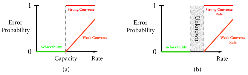
Figure 1: (Color online) Weak converse versus strong converse rates for channels in which (a) the classical capacity is exactly known (such as the pure-loss bosonic channel [9, 34]), and (b) only lower bounds and upper bounds are known, while the exact classical capacity is not known (such as the thermal channel). In both cases, the figures illustrate the idea that the error probability converges to one in the limit of many channel uses if a communication rate corresponds to a strong converse rate, whereas establishing a communication rate as a weak converse rate suggests that there exists room for a trade-off between communication rate and error proability. Achievable rates are such that there exists a communication scheme whose error probability converges to zero in the limit of many channel uses.

2 Summary of results

We now give a brief summary of the present paper’s two main contributions:

1. Following [34], we begin by showing that a strong converse theorem need not hold for the classical capacity of the thermal noise channel and the additive noise channel whenever there is only a mean photon number constraint.

2. In light of the above observation and again following [34], we impose instead a maximum photon number constraint, in such a way that nearly all of the “shadow” of the average density operator for a given code is required to be on a subspace with photon number no larger than a particular number, so that the shadow outside this subspace vanishes in the limit of many channel uses. Under such a maximum photon number constraint, we demonstrate that several previously known upper bounds [7, 12, 19, 11] on the classical capacity of the thermal and additive noise bosonic channels correspond to strong converse rates.

The present paper is organized as follows. In Section 3, we review several preliminary ideas, including mathematical definitions of the thermal noise channel and additive noise channels and structural decompositions of them that are useful in our work. We also present the basic notions of the quantum Rényi entropy and its relation with smooth min-entropy [29]. Section 4 illustrates a simple proof that the strong converse need not hold with only a mean photon number constraint for the above two bosonic channels, following the approach given in [34]. In Section 5, we instead impose a maximum photon number constraint and prove that several previously known upper bounds [7, 12, 19, 11] on the classical capacity of the thermal noise channel and the additive noise channel are actually strong converse rates. Section 6 contains some concluding remarks and an outlook for future research, in particular the implications of our results for other noisy bosonic channels.

3 Preliminaries

3.1 Thermal noise channel

The thermal noise channel is represented by a Gaussian completely positive trace-preserving (CPTP) map—i.e., it evolves Gaussian input states to Gaussian output states [33]. The thermal channel can be modeled by a beamsplitter of transmissivity $\eta$ that couples the input signal with a thermal state of mean photon number $N_{B}$. The parameter $\eta\in[0,1]$ characterizes the fraction of input photons that make it to the output on average. The special case $N_{B}=0$ (zero-temperature reservoir) corresponds to the pure-loss bosonic channel $\mathcal{E}_{\eta,0}$, in which each input photon has a probability $\eta$ of reaching the output.

The beamsplitter transformation corresponding to the thermal channel can be written as the following Heisenberg evolution of the signal mode operator $\hat{a}$ and the environmental mode operator $\hat{b}$:

$$\hat{a} \longrightarrow\sqrt{\eta}\hat{a}+\sqrt{1-\eta}\hat{b}\,,$$

$$\hat{b} \longrightarrow-\sqrt{1-\eta}\hat{a}+\sqrt{\eta}\hat{b}\,.$$ (1)

Tracing out the environmental mode $\hat{b}$ yields the following CPTP map $\mathcal{E}_{\eta,N_{B}}$ for the thermal noise channel:

$$\mathcal{E}_{\eta,N_{B}}=\text{Tr}_{\hat{b}}\left[U(\rho_{a}\otimes\rho_{b})U^{\dagger}\right],$$ (2)

where $\rho_{a}$ and $\rho_{b}$ correspond to the input state and the environmental thermal state, respectively, and the unitary $U$ can be inferred from the transformation in (1). The thermal state $\rho_{b}$ is equivalent to an isotropic Gaussian mixture of coherent states with average photon number $N_{B}\geq 0$ [6]:

$$\rho_{b}=\int d^{2}\alpha\,\frac{\exp(-|\alpha|^{2}/N_{B})}{\pi N_{B}}\,|\alpha\rangle\langle\alpha|=\frac{1}{(N_{B}+1)}\sum_{l=0}^{\infty}\left(\frac{N_{B}}{N_{B}+1}\right)^{l}|l\rangle\langle l|.$$ (3)

As an example, we can see that a vacuum state at the input of the thermal channel produces the following thermal state at the output:

$$\mathcal{E}_{\eta,N_{B}}(|0\rangle\langle 0|)=\frac{1}{\left((1-\eta)N_{B}+1\right)}\sum_{l=0}^{\infty}\left(\frac{(1-\eta)N_{B}}{(1-\eta)N_{B}+1}\right)^{l}|l\rangle\langle l|.$$ (4)

Despite extensive efforts to find the classical capacity of the thermal channel [17, 9, 7, 12, 20, 18, 19, 11], it is still unknown. However, a few upper and lower bounds on it are now known. Holevo and Werner have shown that the classical capacity $C(\mathcal{E}_{\eta,N_{B}})$ of the thermal noise channel $\mathcal{E}_{\eta,N_{B}}$ satisfies [17]

$$C(\mathcal{E}_{\eta,N_{B}})\geq g(\eta N_{S}+(1-\eta)N_{B})-g((1-\eta)N_{B}),$$ (5)

where

$$g(x)\equiv(x+1)\log_{2}(x+1)-x\log_{2}x$$ (6)

is the entropy of a bosonic thermal state with mean photon number $x$. They established this lower bound by proving that coherent-state coding schemes achieve the communication rate on the RHS of (5). It has been conjectured that the above lower bound is equal to the classical capacity of the thermal noise channel, provided that a certain minimum output entropy conjecture is true [7]. The results of [7, 12] establish the following upper bound on the classical capacity of the thermal bosonic channel:

$$C(\mathcal{E}_{\eta,N_{B}})\leq g(\eta N_{S}+(1-\eta)N_{B})-\log_{2}(1+2(1-\eta)N_{B}).$$ (7)

This upper bound lies within 1.45 bits of the lower bound in (5). Koenig and Smith determined tight upper bounds on the classical capacity of the thermal noise channel whenever $\eta=1/2$ [18, 20], by proving a quantum entropy power inequality. They also established the following upper bound on the classical capacity $C(\mathcal{E}_{\eta,N_{B}})$ [19]:

$$C(\mathcal{E}_{\eta,N_{B}})\leq g(\eta N_{S}/[(1-\eta)N_{B}+1]).$$ (8)

This latter bound is also within 1.45 bits of the lower bound in (5).

In this paper, we show that both of the upper bounds in (7) and (8) correspond to strong converse rates.

3.2 Additive noise channel

The additive noise channel is specified by the following CPTP map:

$$\mathcal{N}_{\bar{n}}(\rho)\equiv\int d^{2}\alpha\,P_{\bar{n}}(\alpha)\,D(\alpha)\rho D^{\dagger}(\alpha),$$ (9)

where $P_{\bar{n}}(\alpha)=\exp\left(-|\alpha|^{2}/\bar{n}\right)/(\pi\bar{n})$ and $D(\alpha)\equiv\exp(\alpha\hat{a}^{\dagger}-\alpha^{*}\hat{a})$ is a displacement operator for the input signal mode $\hat{a}$. The Gaussian probability distribution $P_{\bar{n}}(\alpha)$ determines the random displacement of the signal mode $\hat{a}$ in phase space. The variance $\bar{n}$ of this distribution completely characterizes the additive noise channel $\mathcal{N}_{\bar{n}}$, and it represents the number of noise photons added to the mode $\hat{a}$ by the channel [13]. For $\bar{n}=0$, the CPTP map in (9) reduces to the identity channel, while for $\bar{n}>0$, noise photons are injected into the channel. As an example, we can see that the action of the classical noise channel $\mathcal{N}_{\bar{n}}$ on a vacuum-state input produces a thermal-state output:

$$\mathcal{N}_{\bar{n}}(|0\rangle\langle 0|)=\frac{1}{\bar{n}+1}\sum_{l=0}^{\infty}\left(\frac{\bar{n}}{\bar{n}+1}\right)^{l}|l\rangle\langle l|.$$ (10)

Since the additive noise channel can be obtained from the thermal noise channel in the limit $\eta\rightarrow 1$ and $N_{B}\rightarrow\infty$, with $(1-\eta)N_{B}\rightarrow\bar{n}$ [7] (see also Appendix B for a review of this), many results regarding the thermal channel apply to the additive noise channel as well. For example, we obtain the following bounds on the classical capacity of the additive noise channel $\mathcal{N}_{\bar{n}}$ simply by taking the aforementioned limit in (5), (7), and (8), respectively:

$$C(\mathcal{N}_{\bar{n}}) \geq g(N_{S}+\bar{n})-g(\bar{n})\,,$$ (11)

$$C(\mathcal{N}_{\bar{n}}) \leq g(N_{S}+\bar{n})-\log_{2}(1+2\bar{n})\,,$$ (12)

$$C(\mathcal{N}_{\bar{n}}) \leq g(N_{S}/[\bar{n}+1])\,.$$ (13)

This last bound easily follows from (8), but as far as we can tell, it appears to be new.

In this paper, we prove that both of the upper bounds in (12) and (13) correspond to strong converse rates.

3.3 Structural decompositions

Both the thermal and additive noise channels can be decomposed as a concatenation of other channels [8, 7, 2, 5], and these decompositions are helpful in establishing upper bounds on capacity. We briefly review these decompositions in this section and, for convenience, give a full proof of them in Appendix B using the symplectic formalism [17, 33]. The thermal noise channel $\mathcal{E}_{\eta,N_{B}}$ can be regarded as the application of the additive noise channel $\mathcal{N}_{(1-\eta)N_{B}}$ to the output of the pure-loss bosonic channel $\mathcal{E}_{\eta,0}$ [7]:

$$\mathcal{E}_{\eta,N_{B}}(\rho)=\left(\mathcal{N}_{(1-\eta)N_{B}}\circ\mathcal{E}_{\eta,0}\right)(\rho).$$ (14)

The following alternative composition rule holds for the thermal noise channel [2] (see also [5] and [19]):

$$\mathcal{E}_{\eta,N_{B}}(\rho)=\left(\mathcal{A}_{G_{1}}\circ\mathcal{E}_{\eta_{1},0}\right)(\rho),$$ (15)

where $\mathcal{A}_{G_{1}}$ is an amplifier channel with gain $G_{1}=(1-\eta)N_{B}+1$ and $\mathcal{E}_{\eta_{1},0}$ is the pure-loss bosonic channel with transmissivity $\eta_{1}=\eta/G_{1}$. This means that the thermal noise channel $\mathcal{E}_{\eta,N_{B}}$ can be viewed as a cascade of the above two channels, in which the input state is propagated through the pure-loss bosonic channel and followed by the amplifier channel. Taking the limits $\eta\rightarrow 1$ and $N_{B}\rightarrow\infty$, with $(1-\eta)N_{B}\rightarrow\bar{n}$, we obtain from (15) the following composition rule for the additive noise channel [8]:

$$\mathcal{N}_{\bar{n}}(\rho)=(\mathcal{A}_{\bar{n}+1}\circ\mathcal{E}_{\frac{1}{\bar{n}+1},0})(\rho)\,.$$ (16)

3.4 Quantum Rényi entropy and smooth min-entropy

The quantum Rényi entropy $H_{\alpha}(\rho)$ of a density operator $\rho$ is defined for $0<\alpha<\infty$, $\alpha\neq 1$ as

$$H_{\alpha}(\rho)\equiv\frac{1}{1-\alpha}\log_{2}\operatorname{Tr}[\rho^{\alpha}]\,.$$ (17)

It is a monotonic function of the “$\alpha$-purity” $\operatorname{Tr}[\rho^{\alpha}]$, and the von Neumann entropy $H(\rho)$ is recovered from it in the limit $\alpha\rightarrow 1$:

$$\lim_{\alpha\rightarrow 1}H_{\alpha}(\rho)=H(\rho)\equiv-\operatorname{Tr}[\rho\log_{2}\rho]\,.$$

The min-entropy is recovered from it in the limit as $\alpha\rightarrow\infty$:

$$\lim_{\alpha\rightarrow\infty}H_{\alpha}(\rho)=H_{\min}\left(\rho\right)\equiv-\log_{2}\left\|\rho\right\|_{\infty},$$

where $\left\|\rho\right\|_{\infty}$ is the infinity norm of $\rho$. For an additive noise channel $\mathcal{N}_{\bar{n}}$, the Rényi entropy $H_{\alpha}(\mathcal{N}_{\bar{n}}(\rho))$ for $\alpha\in\{2,3,\ldots\}$ achieves its minimum value when the input $\rho$ is the vacuum state $|0\rangle$ [12]:

$$\min_{\rho}H_{\alpha}(\mathcal{N}_{\bar{n}}(\rho))=H_{\alpha}(\mathcal{N}_{\bar{n}}(|0\rangle\langle 0|))=\frac{\log_{2}[(\bar{n}+1)^{\alpha}-\bar{n}^{\alpha}]}{\alpha-1}\,.$$ (18)

Similarly, for the thermal noise channel $\mathcal{E}_{\eta,N_{B}}$, the Rényi entropy $H_{\alpha}(\mathcal{E}_{\eta,N_{B}}(\rho))$ for $\alpha\in\{2,3,\ldots\}$ achieves its minimum value when the input $\rho$ is the vacuum state $|0\rangle$ [12]:

$$\min_{\rho}H_{\alpha}(\mathcal{E}_{\eta,N_{B}}(\rho))=H_{\alpha}(\mathcal{E}_{\eta,N_{B}}(|0\rangle\langle 0|))=\frac{\log_{2}[((1-\eta)N_{B}+1)^{\alpha}-((1-\eta)N_{B})^{\alpha}]}{\alpha-1}\,.$$ (19)

One of the most important questions in quantum information theory is whether the vacuum input still gives the minimum output Rényi entropy for other values of $\alpha$ (with the case $\alpha=1$ being of especial importance [7]).

An elegant generalization of the Rényi entropy is the smooth Rényi entropy, first introduced by Renner and Wolf for classical probability distributions [28]. The results there were further generalized to the quantum case (density operators) by considering the set $\mathcal{B}^{\varepsilon}(\rho)$ of density operators $\tilde{\rho}$ that are $\varepsilon$-close to $\rho$ in trace distance for $\varepsilon\geq 0$ [27]. The $\varepsilon$-smooth quantum Rényi entropy of order $\alpha$ of a density operator $\rho$ is defined as [27]

$$H_{\alpha}^{\varepsilon}(\rho)\equiv\left\{\begin{array}[c]{cc}\inf_{\tilde{\rho}\in\mathcal{B}^{\varepsilon}(\rho)}H_{\alpha}(\tilde{\rho})&0\leq\alpha<1\\ \sup_{\tilde{\rho}\in\mathcal{B}^{\varepsilon}(\rho)}H_{\alpha}(\tilde{\rho})&1<\alpha<\infty\end{array}\right..$$ (20)

In the limit as $\alpha\rightarrow\infty$, we recover the smooth min-entropy of $\rho$ [27, 32]:

$$H_{\min}^{\varepsilon}(\rho)\equiv\sup_{\tilde{\rho}\in\mathcal{B}^{\varepsilon}(\rho)}\left[-\log_{2}\left\|\widetilde{\rho}\right\|_{\infty}\right]\,.$$ (21)

From the above, we see that the following relation holds

$$\inf_{\widetilde{\rho}\in\mathcal{B}^{\varepsilon}\left(\rho\right)}\left\|\widetilde{\rho}\right\|_{\infty}=2^{-H_{\min}^{\varepsilon}\left(\rho\right)}\,.$$ (22)

The following inequality is one of the main results of [28], and it demonstrates a connection between the smooth min-entropy and the Rényi entropy of order $\alpha>1$:

$$H_{\min}^{\varepsilon}\left(\rho\right)\geq H_{\alpha}\left(\rho\right)-\frac{1}{\alpha-1}\log_{2}\left(\frac{1}{\varepsilon}\right).$$ (23)

For convenience, Appendix A reviews the proof of the above inequality from [28].

3.5 Strong converse for the noiseless qubit channel

For a noiseless qubit channel, the argument for the strong converse theorem is rather simple [24, 21], but it plays an important role in this work, so we review it briefly. Suppose that any scheme for classical communication over $n$ noiseless qubit channels consists of an encoding of the message $m$ as a quantum state on $n$ qubits, followed by a decoding POVM $\{\Lambda_{m}\}$. The rate of the code is $R=(\log_{2}M)/n$, and the success probability for a receiver to correctly recover the message is upper bounded as

$$\frac{1}{M}\sum_{m}\text{Tr}\{\Lambda_{m}\rho_{m}\} \leq\frac{1}{M}\sum_{m}\text{Tr}\{\Lambda_{m}\}||\rho_{m}||_{\infty}$$

$$\leq\frac{1}{M}\sum_{m}\text{Tr}\{\Lambda_{m}\}$$

$$=M^{-1}2^{n}$$

$$=2^{-n(R-1)}$$

In the above, we have used that the infinity norm $||\rho_{m}||_{\infty}$ is never larger than one, and $\sum_{m}\Lambda_{m}=I^{\otimes n}$ for any POVM $\{\Lambda_{m}\}$. The above argument demonstrates that for a rate $R>1$, the success probability of any communication scheme decreases exponentially fast to zero with increasing $n$.

The above proof for the noiseless qubit channel highlights an interplay of the success probability of decoding with rate, the dimension of the channel output space, and the purity of the channel (quantified by the infinity norm of the output states of the channel). Our argument for the thermal and additive noise channel can be viewed as a generalization of the above proof.

4 No strong converse under a mean photon number constraint

If we allow the input signal states to have an arbitrarily large number of photons, then the classical capacity of the thermal noise channel is infinite [17]. Thus, in order to have a sensible notion of classical capacity for this channel, we must impose some kind of constraint on the photon number of the signaling states. A common constraint employed in the literature [17, 9] is that the mean number of photons in any codeword transmitted through the channel can be at most $N_{S}\geq 0$ for each use of the channel (mean photon number constraint). In this section, we show that a strong converse does not hold for the classical capacity of the thermal noise and additive noise bosonic channels under such a mean photon number constraint. The arguments presented here for proving this are the same as in [34].

In order to show a violation of the strong converse with a mean photon number constraint, we consider the encoding of a classical message $m$ into $n$-mode coherent-state codewords, where each codeword is independently sampled from an isotropic complex Gaussian distribution with variance $P>N_{S}$ [9, 34]. Let

$$|\alpha^{n}(m)\rangle\equiv|\alpha_{1}(m)\rangle\otimes\cdots\otimes|\alpha_{n}(m)\rangle$$ (24)

denote each of the $n$-mode coherent-state codewords, and we demand that every such codeword in the codebook $\{|\alpha^{n}(m)\rangle\}_{m\in[M]}$ has mean photon number $P>N_{S}$ (letting $M$ be the size of the message set and denoting the message set by $[M]$).

The Holevo-Werner coding theorem [17] states that if we choose these codewords at a rate equal to $\frac{1}{n}\log_{2}\left(M\right)\approx g\left(\eta P+\left(1-\eta\right)N_{B}\right)-g\left(\left(1-\eta\right)N_{B}\right)$ and transmit them over the thermal noise channel $\mathcal{E}_{\eta,N_{B}}$, the receiver can decode them with arbitrarily large success probability. That is, as long as $\frac{1}{n}\log_{2}\left(M\right)\approx g\left(\eta P+\left(1-\eta\right)N_{B}\right)-g\left(\left(1-\eta\right)N_{B}\right)$ and the number $n$ of channel uses is sufficiently large, there exists a measurement $\left\{\Lambda_{m}\right\}_{m\in\left[M\right]}$ and codebook such that

$$\forall m\in\left[M\right]:\text{Tr}\left\{\Lambda_{m}\mathcal{E}_{\eta,N_{B}}^{\otimes n}\left(|\alpha^{n}(m)\rangle\langle\alpha^{n}(m)|\right)\right\}\geq 1-\varepsilon,$$ (25)

for $\varepsilon$ an arbitrarily small positive number.

4.1 No strong converse with mixed-state codewords

What we can do to violate the strong converse is to pick $P$ such that

$$g\left(\eta P+\left(1-\eta\right)N_{B}\right)-g\left(\left(1-\eta\right)N_{B}\right)>g(\eta N_{S}+(1-\eta)N_{B})-\log_{2}(1+2(1-\eta)N_{B}),$$

where the term on the RHS is the upper bound from (7) on the capacity of a thermal channel $\mathcal{E}_{\eta,N_{B}}$ in which we allow for a mean photon number $N_{S}$. We then modify the codebook given above so that each codeword has the following form:

$$\rho_{m}\equiv(1-p)\left|\alpha^{n}(m)\right\rangle\left\langle\alpha^{n}(m)\right|+p(|0\rangle\langle 0|)^{\otimes n},$$ (26)

with $(1-p)P=N_{S}$ (mean photon number constraint) and $0\leq p\leq 1$. Observe that the mean photon number of these modified codewords is equal to $N_{S}$ so that we satisfy the mean photon number constraint. Transmitting these codewords through the thermal noise channel gives the state

$$\mathcal{E}_{\eta,N_{B}}^{\otimes n}\left(\rho_{m}\right).$$

The success probability for correctly decoding the codewords with the decoding measurement $\{\Lambda_{m}\}$ for the original code is then

$$\operatorname{Tr}\{\Lambda_{m}\mathcal{E}_{\eta,N_{B}}^{\otimes n}\left(\rho_{m}\right)\} \geq(1-p)\operatorname{Tr}\{\Lambda_{m}\mathcal{E}_{\eta,N_{B}}^{\otimes n}\left(\left|\alpha^{n}(m)\right\rangle\left\langle\alpha^{n}(m)\right|\right)\}$$ (27)

$$\geq(1-p)(1-\varepsilon).$$ (28)

The last inequality follows from (25). The inequality in (28) proves that the success probability need not converge to zero in the limit of many channel uses for a rate larger than the upper bound on the classical capacity from (7) under a mean photon number constraint on each codeword in the codebook. A very similar argument proves that the strong converse need not hold for the classical capacity of the additive noise channel under only a mean photon number constraint.

4.2 No strong converse with pure-state codewords

In this section, we show that the the classical capacity for the thermal noise and the additive noise channels need not obey a strong converse when only a mean photon number constraint is imposed, even when restricting to pure-state codewords. The argument is again similar to that in [34]. This result is demonstrated by considering the rate to be larger than the upper bound in (8) for the thermal noise channel.

We follow the arguments in [34] and make use of an ancillary single photon to purify the mixed-state codewords in (26) to be as follows:

$$|\gamma_{p}(m)\rangle\equiv\sqrt{(1-p)}\left|\alpha^{n}(m)\right\rangle|0\rangle+\sqrt{p}|0\rangle^{\otimes n}|1\rangle.$$

This additional mode has a negligible effect on the code parameters.

Following [34], we can now show that the average number of photons in each codeword above is equal to

$${\operatorname{Tr}\left\{\left(\frac{1}{n+1}\sum_{i=1}^{n+1}\hat{a}_{i}^{\dagger}\hat{a}_{i}\right)|\gamma_{p}(m)\rangle\langle\gamma_{p}(m)|\right\}=(1-p)\frac{nP}{n+1}+p\frac{1}{n+1}.}$$

Thus, we can set $p$ and $n$ such that the mean number of photons is equal to $N_{S}$ (mean photon number constraint). It now follows by using the argument in (28) that the success probability of correctly decoding the message is larger than $(1-p)(1-\varepsilon)$ (the receiver simply traces over the last mode and performs the POVM $\left\{\Lambda_{m}\right\}$). This proves that a strong converse need not hold for the classical capacity of the thermal channel under a mean photon number constraint, even when restricting to pure-state codewords. Similar arguments can be used to show a similar result for the additive noise channel.

5 Strong converse rates under a maximum photon number constraint

In light of the results in the previous section, we can only hope that a strong converse theorem holds under some alternative photon number constraint. Let $\rho_{m}$ denote a codeword of any code that we wish to transmit through the thermal noise channel $\mathcal{E}_{\eta,N_{B}}$ with transmissivity $\eta$ and the noise photon number $N_{B}$. Following [34], we impose a maximum photon-number constraint, by demanding that the average code-density operator $\frac{1}{M}\sum_{m}\rho_{m}$ ($M$ is the total number of messages) has a large shadow onto a subspace with photon number no larger than some fixed amount $nN_{S}$. In more detail, we define a photon number cutoff projector $\Pi_{L}$ projecting onto a subspace of $n$ bosonic modes such that the total photon number is no larger than $L$:

$$\Pi_{L}\equiv\sum_{a_{1},\ldots,a_{n}:\sum_{i}a_{i}\leq L}|a_{1}\rangle\langle a_{1}|\otimes\ldots\otimes|a_{n}\rangle\langle a_{n}|,$$ (29)

where $|a_{i}\rangle$ is a photon number state of photon number $a_{i}$. We demand that the following maximum photon number constraint is satisfied

$$\frac{1}{M}\sum_{m}\text{Tr}\left\{\Pi_{\left\lceil nN_{S}\right\rceil}\rho_{m}\right\}\geq 1-\delta_{1}(n),$$ (30)

where $\delta_{1}(n)$ is a function that decreases to zero as $n$ increases.

A useful bound for us is that the rank of the photon number cutoff projector $\Pi_{\lceil nN_{S}\rceil}$ cannot be any larger than $2^{n[g(N_{S})+\delta]}$ and $\delta\geq\frac{1}{n}(\log_{2}e+\log_{2}(1+\frac{1}{N_{S}}))$ (Lemma 3 in Ref. [34]), i.e.,

$$\text{Tr}\left\{\Pi_{\lceil nN_{S}\rceil}\right\}\leq 2^{n[g(N_{S})+\delta]}.$$ (31)

The constant $\delta$ can be chosen to be an arbitrarily small positive constant by taking $n$ large enough.

In what follows, we prove that several previously known upper bounds [7, 12, 19, 11] on the classical capacity of the thermal and additive noise channels are actually strong converse rates.

5.1 Koenig-Smith bound is a strong converse rate for the thermal channel

Theorem 1 ((8) is a strong converse rate for $\mathcal{E}_{\eta,N_{B}}$)

For the thermal noise channel $\mathcal{E}_{\eta,N_{B}}$, the average success probability of any code satisfying (30) is bounded as follows:

$$\frac{1}{M}\sum_{m}\operatorname{Tr}\{\Lambda_{m}\mathcal{E}_{\eta,N_{B}}^{\otimes n}(\rho_{m})\}\leq 2^{-n(R-g\left(\eta N_{S}/[(1-\eta)N_{B}+1]\right)-\delta_{2}-\delta_{3})}+2\sqrt{\delta_{1}(n)+\delta_{4}(n)+2\sqrt{\delta_{1}(n)}},$$

where $\mathcal{E}_{\eta,N_{B}}^{\otimes n}$ denotes $n$ instances of the thermal channel, $\delta_{1}(n)$ is defined in (30), $\delta_{2},\delta_{3}$ are arbitrarily small positive constants, and $\delta_{4}(n)$ is a function decreasing to zero as $n$ increases. Thus, for any rate $R>g\left(\eta N_{S}/[(1-\eta)N_{B}+1]\right)+\delta_{2}+\delta_{3}$, (note that we can pick $\delta_{2}$ and $\delta_{3}$ small enough) the success probability of any family of codes satisfying (30) decreases to zero in the limit of large $n$.

Proof. We can consider the thermal noise channel $\mathcal{E}_{\eta,N_{B}}$ as a cascade of a pure-loss bosonic channel $\mathcal{E}_{\eta_{1},0}$ followed by an amplifier channel $\mathcal{A}_{G_{1}}$ (recall the discussion in Section 3.3):

$$\mathcal{E}_{\eta,N_{B}}(\rho)=\left(\mathcal{A}_{G_{1}}\circ\mathcal{E}_{\eta_{1},0}\right)(\rho),$$ (32)

where the gain of the amplifier channel is $G_{1}=(1-\eta)N_{B}+1$ and the pure-loss bosonic channel has transmissivity ${\eta}_{1}=\eta/G_{1}$. Let $N_{S}^{\prime}\equiv N_{S}/[(1-\eta)N_{B}+1]$.

The average success probability of correctly decoding any code satisfying (30) can then be written with the above decomposition rule and bounded as

$$\frac{1}{M}\sum_{m}\text{Tr}\{\Lambda_{m}\mathcal{E}_{\eta,N_{B}}^{\otimes n}(\rho_{m})\}$$

$$=\frac{1}{M}\sum_{m}\text{Tr}\{\Lambda_{m}(\mathcal{A}_{{G}_{1}}^{\otimes n}\circ\mathcal{E}_{\eta_{1},0}^{\otimes n})(\rho_{m})\}$$

$$=\frac{1}{M}\sum_{m}\text{Tr}\left\{\left(\mathcal{A}_{{G}_{1}}^{\otimes n}\right)^{{\dagger}}\left(\Lambda_{m}\right)\mathcal{E}_{\eta_{1},0}^{\otimes n}(\rho_{m})\right\}$$

$$\leq\frac{1}{M}\sum_{m}\text{Tr}\left\{\left(\mathcal{A}_{{G}_{1}}^{\otimes n}\right)^{{\dagger}}\left(\Lambda_{m}\right)\Pi_{\lceil n(\eta N_{s}^{\prime}+\delta_{2})\rceil}\mathcal{E}_{\eta_{1},0}^{\otimes n}(\rho_{m})\Pi_{\lceil n(\eta N_{s}^{\prime}+\delta_{2})\rceil}\right\}$$

$$\ \ \ \ \ \ +\frac{1}{M}\sum_{m}\left\|\mathcal{E}_{\eta_{1},0}^{\otimes n}(\rho_{m})-\Pi_{\lceil n(\eta N_{s}^{\prime}+\delta_{2})\rceil}\mathcal{E}_{\eta_{1},0}^{\otimes n}(\rho_{m})\Pi_{\lceil n(\eta N_{s}^{\prime}+\delta_{2})\rceil}\right\|_{1}$$

$$\leq\frac{1}{M}\sum_{m}\text{Tr}\left\{\left(\mathcal{A}_{{G}_{1}}^{\otimes n}\right)^{{\dagger}}\left(\Lambda_{m}\right)(\Pi_{\lceil n(\eta N_{s}^{\prime}+\delta_{2})\rceil}\mathcal{E}_{\eta_{1},0}^{\otimes n}(\rho_{m})\Pi_{\lceil n(\eta N_{s}^{\prime}+\delta_{2})\rceil})\right\}$$

$$\ \ \ \ \ \ +2\sqrt{\delta_{1}(n)+\delta_{4}(n)+2\sqrt{\delta_{1}(n)}}.$$ (33)

The first equality is obtained by using the decomposition rule stated above. The second equality follows by defining $\left(\mathcal{A}_{{G}_{1}}^{\otimes n}\right)^{{\dagger}}$ as the adjoint of $\mathcal{A}_{{G}_{1}}^{\otimes n}$. The first inequality is a special case of the inequality

$$\operatorname{Tr}\{\Lambda\sigma\}\leq\text{Tr}\{\Lambda\rho\}+||\rho-\sigma||_{1},$$ (34)

which holds for $0\leq\Lambda\leq I$, $\rho,\sigma\geq 0$, and $\operatorname{Tr}\{\rho\},\operatorname{Tr}\{\sigma\}\leq 1$. The second inequality follows from a variation of the Gentle Measurement Lemma [26, 36] for ensembles, which states that $\sum_{x}p_{X}(x)||\rho_{x}-\sqrt{\Lambda}\rho_{x}\sqrt{\Lambda}||_{1}\leq 2\sqrt{\epsilon}$ for an ensemble $\{p_{X}(x),\rho_{x}\}$ where $\sum_{x}p_{X}\operatorname{Tr}\{\Lambda\rho_{x}\}\geq 1-\varepsilon$ and $0\leq\varepsilon\leq 1$. It also follows from an application of Lemma 4 of [34], with $\delta_{4}(n)$ chosen as given there.

We now focus on the first term in the above expression to obtain the upper bound in the statement of the theorem:

$$\frac{1}{M}\sum_{m}\operatorname{Tr}\{\left(\mathcal{A}_{{G}_{1}}^{\otimes n}\right)^{{\dagger}}\left(\Lambda_{m}\right)(\Pi_{\lceil n(\eta N_{s}^{\prime}+\delta_{2})\rceil}\mathcal{E}_{\eta_{1},0}^{\otimes n}(\rho_{m})\Pi_{\lceil n(\eta N_{s}^{\prime}+\delta_{2})\rceil})\}$$ (35)

$$\leq\frac{1}{M}\sum_{m}\operatorname{Tr}\{\Pi_{\lceil n(\eta N_{s}^{\prime}+\delta_{2})\rceil}\left(\mathcal{A}_{{G}_{1}}^{\otimes n}\right)^{{\dagger}}(\Lambda_{m})\Pi_{\lceil n(\eta N_{s}^{\prime}+\delta_{2})\rceil}\}$$

$$=M^{-1}\operatorname{Tr}\{\Pi_{\lceil n(\eta N_{s}^{\prime}+\delta_{2})\rceil}\}$$

$$\leq 2^{-n(R-g(\eta N_{S}^{\prime})-\delta_{2}-\delta_{3})}.$$

The first inequality follows since $||\mathcal{E}_{\eta_{1},0}^{\otimes n}(\rho_{m})||_{\infty}\leq 1$. The first equality is a consequence of the fact that $\sum_{m}\Lambda_{m}=I$ for any POVM $\{\Lambda_{m}\}$ and that the adjoint of any CPTP map is unital. The last equality follows from (31) and from the fact that the rate $R=(\log_{2}M)/n$. Thus, we arrive at the statement of the theorem—if the rate $R>g(\eta N_{s}^{\prime})$, we can choose the constants $\delta_{2},\delta_{3}$ to be arbitrarily small such that $R>g(\eta N_{s}^{\prime})+\delta_{2}+\delta_{3}$, and the success probability decreases to zero in the limit of $n\rightarrow\infty$.   

5.2 Koenig-Smith-like bound is a strong converse rate for the additive noise channel

Recall that the additive noise channel $\mathcal{N}_{\bar{n}}$ can be realized as a pure-loss bosonic channel $\mathcal{E}_{\eta_{2},0}$ with transmissivity $\eta_{2}=1/(\bar{n}+1)$ followed by an amplifier channel $\mathcal{A}_{G_{2}}$ with gain $G_{2}=(\bar{n}+1)$ (see Appendix B for details), i.e.,

$$\mathcal{N}_{\bar{n}}=\left(\mathcal{A}_{G_{2}}\circ\mathcal{E}_{\eta_{2},0}\right)(\rho)\equiv\mathcal{A}_{G_{2}}\left(\mathcal{E}_{\eta_{2},0}(\rho)\right)\,.$$ (36)

Then it follows from Theorem 1, by making the replacement $(1-\eta)N_{B}\rightarrow\bar{n}$ in the thermal noise channel results, that the upper bound in (13) is a strong converse rate for the additive noise channel. That is, the average success probability of correctly decoding any code under a maximum photon number constraint decreases to zero as $n$ becomes large for any rate $R>g\left(N_{S}/(\bar{n}+1)\right)$.

5.3 Giovannetti et al. bound is a strong converse rate for the thermal channel

We now prove that the upper bound in (7) corresponds to a strong converse rate for the thermal channel under a maximum photon number constraint. In order to prove that, it is essential to show that if most of the probability mass of the input state is in a subspace with photon number no larger than $nN_{S}$, then the most of the probability mass of the thermal channel output is in a subspace with photon number no larger than $n(\eta N_{S}+\left(1-\eta\right)N_{B})$.

Lemma 1

Let $\rho^{(n)}$ denote a density operator on $n$ modes satisfying

$$\operatorname{Tr}\{\Pi_{\lceil nN_{S}\rceil}\rho^{(n)}\}\geq 1-\delta_{1}(n),$$

where $\delta_{1}(n)$ is a function of $n$ decreasing to zero as $n$ increases. Then

$$\operatorname{Tr}\{\Pi_{\lceil n(\eta N_{S}+(1-\eta)N_{B})+\delta_{5})\rceil}\mathcal{E}_{\eta,N_{B}}^{\otimes n}(\rho^{(n)})\}\geq 1-\delta_{1}(n)-2\sqrt{\delta_{1}(n)}-\delta_{6}(n),$$

where $\mathcal{E}_{\eta,N_{B}}^{\otimes n}$ represents $n$ instances of the thermal noise channel, $\delta_{5}$ is an arbitrarily small positive constant, and $\delta_{6}(n)$ is a function of $n$ decreasing to zero as $n\rightarrow\infty$.

Proof. Recall the structural decomposition of the thermal noise channel from (14):

$$\mathcal{E}_{\eta,N_{B}}(\rho)=\left(\mathcal{N}_{(1-\eta)N_{B}}\circ\mathcal{E}_{\eta,0}\right)(\rho).$$

This decomposition states that a thermal noise channel with transmissivity $\eta$ and noise power $N_{B}$ can be realized as a concatenation of a pure-loss channel of transmissivity $\eta$ followed by a classical noise channel $\mathcal{N}_{\left(1-\eta\right)N_{B}}$. Thus, a photon number state $\left|k\right\rangle\left\langle k\right|$ input to the thermal noise channel leads to an output of the following form:

$$\mathcal{E}_{\eta,N_{B}}\left(\left|k\right\rangle\left\langle k\right|\right)=\sum_{m=0}^{k}p_{m}\mathcal{N}_{\left(1-\eta\right)N_{B}}\left(\left|m\right\rangle\left\langle m\right|\right),$$ (37)

where

$$p_{m}=\binom{k}{m}\eta^{m}\left(1-\eta\right)^{k-m}.$$

The classical noise channel has the following action on a photon number state [7, 3]:

$$\mathcal{N}_{\left(1-\eta\right)N_{B}}\left(\left|m\right\rangle\left\langle m\right|\right)=\sum_{l=0}^{\infty}\lambda_{l}\left|l\right\rangle\left\langle l\right|,$$

where

$$\lambda_{l}=\sum_{j=0}^{\min\left(l,m\right)}\binom{l}{j}\binom{m}{j}\frac{\left(\left(1-\eta\right)N_{B}\right)^{m+l-2j}}{\left(1+\left(1-\eta\right)N_{B}\right)^{m+l+1}}.$$ (38)

Important properties of the distribution $\lambda_{l}$ are that it decays exponentially to zero as $l\rightarrow\infty$ and has finite second moment. It follows from (37) that

$$\mathcal{E}_{\eta,N_{B}}\left(\left|k\right\rangle\left\langle k\right|\right)=\sum_{l=0}^{\infty}\left[\sum_{m=0}^{k}\sum_{j=0}^{\min\left(l,m\right)}\binom{k}{m}\eta^{m}\left(1-\eta\right)^{k-m}\binom{l}{j}\binom{m}{j}\frac{\left(\left(1-\eta\right)N_{B}\right)^{m+l-2j}}{\left(1+\left(1-\eta\right)N_{B}\right)^{m+l+1}}\right]\left|l\right\rangle\left\langle l\right|.$$

The eigenvalues above represent a distribution over photon number states at the output of the thermal noise channel $\mathcal{E}_{\eta,N_{B}}$, which we can write as a probability distribution over $l$ given the input $k$:

$$p\left(l|k\right)=\sum_{m=0}^{k}\sum_{j=0}^{\min\left(l,m\right)}\binom{k}{m}\eta^{m}\left(1-\eta\right)^{k-m}\binom{l}{j}\binom{m}{j}\frac{\left(\left(1-\eta\right)N_{B}\right)^{m+l-2j}}{\left(1+\left(1-\eta\right)N_{B}\right)^{m+l+1}}.$$ (39)

The above probability distribution has its mean equal to $\eta k+\left(1-\eta\right)N_{B}$. The reason is that the mean photon number of the input is equal to $k$, and the mean photon number of the output is equal to a linear combination of the input mean photon numbers. Furthermore, it inherits from the distribution in (38) the properties of having finite second moment and an exponential decay to zero as $l\rightarrow\infty$.

Supposing that the input state satisfies the maximum photon-number constraint in (30), we now observe that

$$\text{Tr}\left\{\left(\Pi_{\left\lceil n\left(\eta N_{S}+\left(1-\eta\right)N_{B}+\delta_{5}\right)\right\rceil}\right)\mathcal{E}_{\eta,N_{B}}^{\otimes n}\left(\rho^{\left(n\right)}\right)\right\}$$

$$\geq\text{Tr}\left\{\left(\Pi_{\left\lceil n\left(\eta N_{S}+\left(1-\eta\right)N_{B}+\delta_{5}\right)\right\rceil}\right)\mathcal{E}_{\eta,N_{B}}^{\otimes n}\left(\Pi_{\left\lceil nN_{S}\right\rceil}\rho^{\left(n\right)}\Pi_{\left\lceil nN_{S}\right\rceil}\right)\right\}-2\sqrt{\delta_{1}}$$ (40)

The inequality follows from the Gentle Measurement Lemma [26, 36]. Since there is photodetection at the output (i.e., the projector $\Pi_{\left\lceil n\left(\eta N_{S}+\left(1-\eta\right)N_{B}+\delta_{5}\right)\right\rceil}$ is diagonal in the number basis), it suffices for us to consider the input $\Pi_{\left\lceil nN_{S}\right\rceil}\rho^{\left(n\right)}\Pi_{\left\lceil nN_{S}\right\rceil}$ to be diagonal in the photon-number basis, and we write this as

$$\rho^{\left(n\right)}=\sum_{a^{n}:\sum_{i}a_{i}\leq\lceil nN_{S}\rceil}p\left(a^{n}\right)\left|a^{n}\right\rangle\left\langle a^{n}\right|,$$

where $\left|a^{n}\right\rangle$ represents strings of photon number states. Continuing, we find that (40) is equal to

$$\sum_{a^{n}:\sum_{i}a_{i}\leq\left\lceil nN_{S}\right\rceil}p\left(a^{n}\right)\text{Tr}\left\{\left(\Pi_{\left\lceil n\left(\eta N_{S}+\left(1-\eta\right)N_{B}+\delta_{5}\right)\right\rceil}\right)\mathcal{E}_{\eta,N_{B}}^{\otimes n}\left(\left|a^{n}\right\rangle\left\langle a^{n}\right|\right)\right\}-2\sqrt{\delta_{1}}$$

$$=\sum_{a^{n}:\sum_{i}a_{i}\leq\left\lceil nN_{S}\right\rceil}p\left(a^{n}\right)\sum_{l^{n}:\sum_{i}l_{i}\leq\left\lceil n\left(\eta N_{S}+\left(1-\eta\right)N_{B}+\delta_{5}\right)\right\rceil}p\left(l^{n}|a^{n}\right)-2\sqrt{\delta_{1}},$$ (41)

where the distribution $p\left(l^{n}|a^{n}\right)\equiv\prod\limits_{i=1}^{n}p\left(l_{i}|a_{i}\right)$ and each $p\left(l_{i}|a_{i}\right)$ is defined from (39).

In order to obtain a lower bound on the expression in (41), we analyze the term

$$\sum_{l^{n}:\sum_{i}l_{i}\leq\left\lceil n\left(\eta N_{S}+\left(1-\eta\right)N_{B}+\delta_{5}\right)\right\rceil}p\left(l^{n}|a^{n}\right)$$ (42)

on its own under the assumption that $\sum_{i}a_{i}\leq\left\lceil nN_{S}\right\rceil$. Let $L_{i}|a_{i}$ denote a conditional random variable with distribution $p\left(l_{i}|a_{i}\right)$, and let $\overline{L^{n}}|a^{n}$ denote the sum random variable:

$$\overline{L^{n}}|a^{n}\equiv\sum_{i}L_{i}|a_{i},$$

so that

$$\sum_{l^{n}:\sum_{i}l_{i}\leq\left\lceil n\left(\eta N_{S}+\left(1-\eta\right)N_{B}+\delta_{5}\right)\right\rceil}p\left(l^{n}|a^{n}\right) =\Pr\left\{\overline{L^{n}}|a^{n}\leq n\left(\eta N_{S}+\left(1-\eta\right)N_{B}+\delta_{5}\right)\right\}$$

$$\geq\Pr\left\{\overline{L^{n}}|a^{n}\leq n\left(\eta\frac{1}{n}\sum_{i}a_{i}+\left(1-\eta\right)N_{B}+\delta_{5}\right)\right\},$$ (43)

where the inequality follows from the constraint $\sum_{i}a_{i}\leq\left\lceil nN_{S}\right\rceil$. Since

$$\mathbb{E}\left\{L_{i}|a_{i}\right\}=\eta a_{i}+\left(1-\eta\right)N_{B},$$

it follows that

$$\mathbb{E}\left\{\overline{L^{n}}|a^{n}\right\}=n\left(\eta\frac{1}{n}\sum_{i}a_{i}+\left(1-\eta\right)N_{B}\right),$$

and so the expression in (43) is the probability that a sum of independent random variables deviates from its mean by no more than $\delta_{5}$.

There are several ways to proceed with bounding the probability in (43) from below. Since all of the random variables $L_{i}|a_{i}$ have finite second moment, we can employ the Chebyshev inequality to bound (43) from below by $1-C/n$, where $C$ is a constant depending on the maximum variance of the $L_{i}$ random variables and the deviation $\delta_{5}$. However, if we would like to prove that there is a stronger rate of convergence, the fact that the random variables are unbounded might seem to be problematic. Nevertheless, one could employ the truncation method detailed in Section 2.1 of [31], in which each random variable $L_{i}|a_{i}$ is split into two parts:

$$\left(L_{i}|a_{i}\right)_{>T} \equiv\left(L_{i}|a_{i}\right)\mathcal{I}\left(\left(L_{i}|a_{i}\right)>T\right),$$

$$\left(L_{i}|a_{i}\right)_{\leq T} \equiv\left(L_{i}|a_{i}\right)\mathcal{I}\left(\left(L_{i}|a_{i}\right)\leq T\right),$$

where $\mathcal{I}\left(\cdot\right)$ is the indicator function and $T$ is a truncation parameter taken to be very large (much larger than $\max_{i}a_{i}$, for example). We can then split the sum random variable into two parts as well:

$$\overline{L^{n}}|a^{n} =\left(\overline{L^{n}}|a^{n}\right)_{>T}+\left(\overline{L^{n}}|a^{n}\right)_{\leq T}$$

$$\equiv\sum_{i}\left(L_{i}|a_{i}\right)_{>T}+\sum_{i}\left(L_{i}|a_{i}\right)_{\leq T}.$$

We can use the union bound to argue that

$$\Pr\left\{\overline{L^{n}}|a^{n}\geq\mathbb{E}\left\{\overline{L^{n}}|a^{n}\right\}+n\delta_{5}\right\}\leq\Pr\left\{\left(\overline{L^{n}}|a^{n}\right)_{>T}\geq\mathbb{E}\left\{\left(\overline{L^{n}}|a^{n}\right)_{>T}\right\}+n\delta_{5}/2\right\}\\ +\Pr\left\{\left(\overline{L^{n}}|a^{n}\right)_{\leq T}\geq\mathbb{E}\left\{\left(\overline{L^{n}}|a^{n}\right)_{\leq T}\right\}+n\delta_{5}/2\right\}.$$ (44)

The idea from here is that for a random variable $L_{i}|a_{i}$ with sufficient decay for large values, we can bound the first probability for $\left(\overline{L^{n}}|a^{n}\right)_{>T}$ from above by $\varepsilon/\delta_{5}$ for $\varepsilon$ an arbitrarily small positive constant (made small by taking $T$ larger) by employing the Markov inequality. We then bound the second probability for $\left(\overline{L^{n}}|a^{n}\right)_{\leq T}$ using a Chernoff bound, since these random variables are bounded. This latter bound has an exponential decay due to the ability to use a Chernoff bound. So, the argument is just to make $\varepsilon$ arbitrarily small by increasing the truncation parameter $T$, and for $n$ large enough, exponential convergence to zero kicks in. We point the reader to Section 2.1 of [31] for more details. By using either approach, we arrive at the following bound:

$$\sum_{l^{n}:\sum_{i}l_{i}\leq\left\lceil n\left(\eta N_{S}+\left(1-\eta\right)N_{B}+\delta_{5}\right)\right\rceil}p\left(l^{n}|a^{n}\right)\geq 1-\delta_{6}(n),$$

where $\delta_{6}(n)$ is a function decreasing to zero as $n\rightarrow\infty$.

Finally, we put this together with (41) to obtain that

$$\operatorname{Tr}\{\Pi_{\lceil n(\eta N_{S}+(1-\eta)N_{B})+\delta_{5})\rceil}\mathcal{E}_{\eta,N_{B}}^{\otimes n}(\rho^{(n)})\}$$

$$\geq\sum_{a^{n}:\sum_{i}a_{i}\leq\left\lceil nN_{S}\right\rceil}p\left(a^{n}\right)\sum_{l^{n}:\sum_{i}l_{i}\leq\left\lceil n\left(\eta N_{S}+\left(1-\eta\right)N_{B}+\delta_{5}\right)\right\rceil}p\left(l^{n}|a^{n}\right)-2\sqrt{\delta_{1}}$$

$$\geq\left(1-\delta_{1}\right)\left(1-\delta_{6}(n)\right)-2\sqrt{\delta_{1}}$$

$$\geq 1-\delta_{1}-\delta_{6}(n)-2\sqrt{\delta_{1}}.$$

 

The above lemma can be extended to the additive noise channel by employing the relation of this channel to the thermal channel (discussed in Section 3.3). For the additive noise channel $\mathcal{N}_{\bar{n}}$, it follows that if the input state is in the subspace with photon number no larger than $nN_{S}$, then the additive noise output is projected with very high probability onto a subspace with photon number no larger than $n(N_{S}+\bar{n})$.

We now proceed to prove that the upper bounds in (7) and (12) are strong converse rates.

Theorem 2 ((7) is a strong converse rate)

The average success probability of any code satisfying (30) is bounded as follows:

$$\frac{1}{M}\sum_{m}\text{Tr}\{\Lambda_{m}\mathcal{E}_{\eta,N_{B}}^{\otimes n}(\rho_{m})\}\\ \leq 2^{-n\left[R-\left[g\left(\eta N_{S}+(1-\eta)N_{B}+\delta_{5}\right)-\log_{2}\left(1+2(1-\eta)N_{B}\right)\right]+\frac{1}{n}\log_{2}\left(n\right)-\delta\right]}\\ +\frac{1}{n}+2\sqrt{\delta_{1}(n)+2\sqrt{\delta_{1}(n)}+\delta_{6}(n)}$$

where $\mathcal{E}_{\eta,N_{B}}^{\otimes n}$ denotes $n$ instances of the thermal channel, and $\delta$ is an arbitrarily small positive constant. Thus, if $R>[g\left(\eta N_{S}+\left(1-\eta\right)N_{B}\right)-\log_{2}\left(1+2(1-\eta)N_{B}\right)]$, then we can pick $\delta$ and $\delta_{5}$ decreasing to zero for large $n$, such that the success probability of any family of codes satisfying (30) decreases to zero as $n\rightarrow\infty$.

Proof. Consider the success probability of any code satisfying the maximum photon-number constraint in (30):

$$\frac{1}{M}\sum_{m}\text{Tr}\{\Lambda_{m}\mathcal{E}_{\eta,N_{B}}^{\otimes n}(\rho_{m})\}.$$

From the assumption that

$$\frac{1}{M}\sum_{m}\text{Tr}\left\{\Pi_{\lceil nN_{S}\rceil}\rho_{m}\right\}\geq 1-\delta_{1}\left(n\right),$$

Lemma 1 allows us to conclude that

$$\frac{1}{M}\sum_{m}\operatorname{Tr}\{\Pi_{\lceil n(\eta N_{S}+(1-\eta)N_{B})+\delta_{5})\rceil}\mathcal{E}_{\eta,N_{B}}^{\otimes n}(\rho_{m})\}\geq 1-\delta_{1}(n)-2\sqrt{\delta_{1}(n)}-\delta_{6}(n),$$

where the functions and constants are as given there. Using the Gentle Measurement Lemma for ensembles [26, 36], we find that

$$\frac{1}{M}\sum_{m}\text{Tr}\{\Lambda_{m}\mathcal{E}_{\eta,N_{B}}^{\otimes n}(\rho_{m})\}$$

$$\leq\frac{1}{M}\sum_{m}\text{Tr}\{\Lambda_{m}\Pi_{\lceil n(\eta N_{S}+(1-\eta)N_{B})+\delta_{5})\rceil}\mathcal{E}_{\eta,N_{B}}^{\otimes n}(\rho_{m})\Pi_{\lceil n(\eta N_{S}+(1-\eta)N_{B})+\delta_{5})\rceil}\}$$

$$\ \ \ \ \ \ +\frac{1}{M}\sum_{m}\left\|\Pi_{\lceil n(\eta N_{S}+(1-\eta)N_{B})+\delta_{5})\rceil}\mathcal{E}_{\eta,N_{B}}^{\otimes n}(\rho_{m})\Pi_{\lceil n(\eta N_{S}+(1-\eta)N_{B})+\delta_{5})\rceil}-\mathcal{E}_{\eta,N_{B}}^{\otimes n}(\rho_{m})\right\|_{1}$$

$$\leq\frac{1}{M}\sum_{m}\text{Tr}\{\Lambda_{m}\Pi_{\lceil n(\eta N_{S}+(1-\eta)N_{B})+\delta_{5})\rceil}\mathcal{E}_{\eta,N_{B}}^{\otimes n}(\rho_{m})\Pi_{\lceil n(\eta N_{S}+(1-\eta)N_{B})+\delta_{5})\rceil}\}$$

$$\ \ \ \ \ \ +2\sqrt{\delta_{1}(n)+2\sqrt{\delta_{1}(n)}+\delta_{6}(n)}$$

We now focus on the term

$$\frac{1}{M}\sum_{m}\text{Tr}\{\Lambda_{m}\Pi_{\lceil n(\eta N_{S}+(1-\eta)N_{B})+\delta_{5})\rceil}\mathcal{E}_{\eta,N_{B}}^{\otimes n}(\rho_{m})\Pi_{\lceil n(\eta N_{S}+(1-\eta)N_{B})+\delta_{5})\rceil}\}$$

$$=\frac{1}{M}\sum_{m}\text{Tr}\{\Pi_{\lceil n(\eta N_{S}+(1-\eta)N_{B})+\delta_{5})\rceil}\Lambda_{m}\Pi_{\lceil n(\eta N_{S}+(1-\eta)N_{B})+\delta_{5})\rceil}\mathcal{E}_{\eta,N_{B}}^{\otimes n}(\rho_{m})\}.$$ (45)

Rather than working with the states $\mathcal{E}_{\eta,N_{B}}^{\otimes n}\left(\rho_{m}\right)$ directly, we consider states $\widetilde{\sigma}_{m}$ that are $\varepsilon$-close in trace distance to $\mathcal{E}_{\eta,N_{B}}^{\otimes n}\left(\rho_{m}\right)$, and this gives the following upper bound on (45):

$$\leq\frac{1}{M}\sum_{m}\text{Tr}\{\Pi_{\lceil n(\eta N_{S}+(1-\eta)N_{B})+\delta_{5})\rceil}\Lambda_{m}\Pi_{\lceil n(\eta N_{S}+(1-\eta)N_{B})+\delta_{5})\rceil}\widetilde{\sigma}_{m}\}+\varepsilon$$

$$\leq\frac{1}{M}\sum_{m}\text{Tr}\{\Pi_{\lceil n(\eta N_{S}+(1-\eta)N_{B})+\delta_{5})\rceil}\Lambda_{m}\Pi_{\lceil n(\eta N_{S}+(1-\eta)N_{B})+\delta_{5})\rceil}\}\left\|\widetilde{\sigma}_{m}\right\|_{\infty}+\varepsilon.$$

Now, this last bound holds regardless of which $\widetilde{\sigma}_{m}$ we pick, so we optimize over all of them that are $\varepsilon$-close to $\mathcal{E}_{\eta,N_{B}}^{\otimes n}\left(\rho_{m}\right)$ (let us denote this set by $\mathcal{B}^{\varepsilon}\left(\mathcal{E}_{\eta,N_{B}}^{\otimes n}\left(\rho_{m}\right)\right)$). This gives the tightest upper bound on the success probability, leading to

$$\frac{1}{M}\sum_{m}\text{Tr}\{\Pi_{\lceil n(\eta N_{S}+(1-\eta)N_{B})+\delta_{5})\rceil}\Lambda_{m}\Pi_{\lceil n(\eta N_{S}+(1-\eta)N_{B})+\delta_{5})\rceil}\mathcal{E}_{\eta,N_{B}}^{\otimes n}(\rho_{m})\}$$

$$\leq\frac{1}{M}\sum_{m}\text{Tr}\{\Pi_{\lceil n(\eta N_{S}+(1-\eta)N_{B})+\delta_{5})\rceil}\Lambda_{m}\Pi_{\lceil n(\eta N_{S}+(1-\eta)N_{B})+\delta_{5})\rceil}\}\inf_{\widetilde{\sigma}_{m}\in\mathcal{B}^{\varepsilon}\left(\mathcal{E}_{\eta,N_{B}}^{\otimes n}\left(\rho_{m}\right)\right)}\left\|\widetilde{\sigma}_{m}\right\|_{\infty}+\varepsilon$$

The quantity $\inf_{\widetilde{\sigma}_{m}\in\mathcal{B}^{\varepsilon}\left(\mathcal{E}_{\eta,N_{B}}^{\otimes n}\left(\rho_{m}\right)\right)}\left\|\widetilde{\sigma}_{m}\right\|_{\infty}$ is related to the smooth min-entropy via

$$\inf_{\widetilde{\sigma}_{m}\in\mathcal{B}^{\varepsilon}\left(\mathcal{E}_{\eta,N_{B}}^{\otimes n}\left(\rho_{m}\right)\right)}\left\|\widetilde{\sigma}_{m}\right\|_{\infty}=2^{-H_{\min}^{\varepsilon}\left(\mathcal{E}_{\eta,N_{B}}^{\otimes n}(\rho_{m})\right)},$$

so we replace the expression above by

$$\frac{1}{M}\sum_{m}\text{Tr}\{\Pi_{\lceil n(\eta N_{S}+(1-\eta)N_{B})+\delta_{5})\rceil}\Lambda_{m}\Pi_{\lceil n(\eta N_{S}+(1-\eta)N_{B})+\delta_{5})\rceil}\}2^{-H_{\min}^{\varepsilon}\left(\mathcal{E}_{\eta,N_{B}}^{\otimes n}(\rho_{m})\right)}+\varepsilon$$

$$\leq\frac{1}{M}\sum_{m}\text{Tr}\{\Pi_{\lceil n(\eta N_{S}+(1-\eta)N_{B})+\delta_{5})\rceil}\Lambda_{m}\Pi_{\lceil n(\eta N_{S}+(1-\eta)N_{B})+\delta_{5})\rceil}\}\sup_{\rho}2^{-H_{\min}^{\varepsilon}\left(\mathcal{E}_{\eta,N_{B}}^{\otimes n}(\rho)\right)}+\varepsilon$$

$$=\frac{1}{M}2^{-\inf_{\rho}H_{\min}^{\varepsilon}\left(\mathcal{E}_{\eta,N_{B}}^{\otimes n}(\rho)\right)}\text{Tr}\{\Pi_{\lceil n(\eta N_{S}+(1-\eta)N_{B})+\delta_{5})\rceil}\}+\varepsilon$$

$$\leq\frac{1}{M}2^{-\inf_{\rho}H_{\min}^{\varepsilon}\left(\mathcal{E}_{\eta,N_{B}}^{\otimes n}(\rho)\right)}2^{n\left[g\left(\eta N_{S}+(1-\eta)N_{B}+\delta_{5}\right)+\delta\right]}+\varepsilon$$

$$\leq 2^{-nR}2^{-\inf_{\rho}H_{2}\left(\mathcal{E}_{\eta,N_{B}}^{\otimes n}(\rho)\right)+\log_{2}\left(\frac{1}{\varepsilon}\right)}2^{n\left[g\left(\eta N_{S}+(1-\eta)N_{B}+\delta_{5}\right)+\delta\right]}+\varepsilon$$

$$=2^{-nR}2^{-n\left[\log_{2}\left(1+2(1-\eta)N_{B})\right)+\frac{1}{n}\log_{2}\left(\frac{1}{\varepsilon}\right)\right]}2^{n\left[g\left(\eta N_{S}+(1-\eta)N_{B}+\delta_{5}\right)+\delta\right]}+\varepsilon.$$

The first inequality follows by taking a supremum over all input states. The first equality follows because $\sum_{m}\Lambda_{m}=I$. The second inequality follows from the upper bound in (31) on the rank of the photon number subspace projector. The last few lines follow by applying the following relation from [29] between the smooth min-entropy $H_{\min}^{\varepsilon}\left(\mathcal{E}_{\eta,N_{B}}^{\otimes n}\left(\rho_{m}\right)\right)$ and the quantum Rényi entropy $H_{\alpha}\left(\mathcal{E}_{\eta,N_{B}}^{\otimes n}\left(\rho_{m}\right)\right)$ in (23) for $\alpha=2$, yielding

$$\inf_{\rho}H_{\min}^{\varepsilon}\left(\mathcal{E}_{\eta,N_{B}}^{\otimes n}\left(\rho_{m}\right)\right) \geq\inf_{\rho}H_{2}\left(\mathcal{E}_{\eta,N_{B}}^{\otimes n}\left(\rho\right)\right)-\log\left(\frac{1}{\varepsilon}\right)$$

$$\geq n\inf_{\omega}H_{2}\left(\mathcal{E}_{\eta,N_{B}}\left(\omega\right)\right)-\log\left(\frac{1}{\varepsilon}\right)$$

$$=n\log_{2}\left(1+2(1-\eta)N_{B}\right)-\log\left(\frac{1}{\varepsilon}\right),$$

where the last two lines above follow from the main result of [7, 12], that the output Rényi entropy of order two is minimized by the $n$-fold tensor-product vacuum state. We now see that we can choose $\varepsilon=\frac{1}{n}$, and we arrive at the following bound

$$2^{-nR}2^{-n\left[\log_{2}\left(1+2(1-\eta)N_{B}\right)+\frac{1}{n}\log_{2}\left(n\right)\right]}2^{n\left[g\left(\eta N_{S}+(1-\eta)N_{B}+\delta_{5}\right)+\delta\right]}+\frac{1}{n}.$$

Putting everything together, we arrive at the following inequality:

$$\frac{1}{M}\sum_{m}\text{Tr}\{\Lambda_{m}\mathcal{E}_{\eta,N_{B}}^{\otimes n}(\rho_{m})\}\\ \leq 2^{-n\left[R-\left[g\left(\eta N_{S}+(1-\eta)N_{B}+\delta_{5}\right)-\log_{2}\left(1+2(1-\eta)N_{B}\right)\right]+\frac{1}{n}\log_{2}\left(n\right)-\delta\right]}\\ +\frac{1}{n}+2\sqrt{\delta_{1}(n)+2\sqrt{\delta_{1}(n)}+\delta_{6}(n)}$$

This upper bound on the success probability demonstrates that for a rate

$$R>\left[g\left(\eta N_{S}+\left(1-\eta\right)N_{B}\right)-\log_{2}\left(1+2(1-\eta)N_{B}\right)\right],$$

we can choose $\delta_{5}$ and $\delta$ small enough so that the success probability decreases to zero in the limit of large $n$.   

5.4 Giovannetti et al. bound is a strong converse rate for the additive noise channel

Using (36), it follows that we can take the limit $(1-\eta)N_{B}\rightarrow\bar{n}$ (with $N_{B}\rightarrow\infty$ and $\eta\rightarrow 1$) to prove that the upper bound in (12) serves as a strong converse rate for the additive noise channel $\mathcal{N}_{\bar{n}}$. The arguments for showing the strong converse rate for the thermal channel then apply for the additive noise channel, and we can say that, for the additive noise channel, the average success probability under a maximum photon number constraint decreases to zero with many channel uses if $R>[g\left(N_{S}+\bar{n}\right)-\log_{2}\left(1+2\bar{n}\right)]$.

6 Conclusion

In this paper, we showed that several previously known upper bounds on the classical capacity for the thermal noise and additive noise channels are actually strong converse rates. We did this by imposing a particular maximum photon number constraint, guaranteeing that the inputs to the channel have almost all of their shadow on a subspace with photon number no larger than $nN_{S}$. The classical capacity of these two channels are not exactly known; however, our results strengthen the interpretation of known upper bounds on the classical capacity of these two channels, so that there is no room for a trade-off between the communication rate and error probability. Besides having an application to proving security in some particular models of cryptography [22], it should be possible to extend our results to multiple-access bosonic channels, i.e., bosonic channels in which two or more senders communicate to a common receiver over a shared channel [38].

Note: After the completion of this work, we discovered very recently that Giovannetti, Holevo, and Garcia-Patron proposed a solution to the long-standing minimum output entropy conjecture [10] (in fact a more general Gaussian optimizer conjecture). Their results imply that the lower bounds in (5) and (11) are in fact upper bounds as well, so that they have identified the classical capacity of these channels. After browsing their proof, we think that it should be possible to combine their results with the development here in order to prove that the rates in (5) and (11) are in fact strong converse rates (so that there is a strong converse theorem for the classical capacity of these channels). In order to arrive at this conclusion, one would need at the very least to extend their development in Section 6 to prove that the minimum output Rényi entropy for all $\alpha\geq 1$ is minimized by the vacuum state. One could then take a similar approach as we did in the last few steps of the proof of Theorem 2. However, this remains the subject of future research.

7 Acknowledgements

We are grateful to Raul Garcia-Patron and Andreas Winter for insightful discussions. BRB would like to acknowledge supports from an Army Research Office grant (W911NF-13-1-0381) and the Charles E. Coates Memorial Research Award Grant from Louisiana State University. MMW is grateful to the Department of Physics and Astronomy at Louisiana State University for startup funds that supported this research.

Appendix A Relation between smooth min-entropy and Rényi entropy

For completeness, we include a proof of the main result of [29]:

Lemma 2

For any random variable $Z$, $\alpha>1$, and $\varepsilon\in\left(0,1\right)$, the following inequality holds

$$H_{\min}^{\varepsilon}\left(Z\right)\geq H_{\alpha}\left(Z\right)-\frac{1}{\alpha-1}\log\left(\frac{1}{\varepsilon}\right).$$

Proof. Let $p_{Z}\left(z\right)$ be a probability distribution for $Z$. Suppose without loss of generality that the elements of the distribution are in decreasing order. In order to prove this inequality, we should find another distribution $q_{Z}\left(z\right)$ such that $\frac{1}{2}\sum_{z}\left|p_{Z}\left(z\right)-q_{Z}\left(z\right)\right|=\varepsilon$ and for which the inequality holds. We will choose it to have the same support as $p_{Z}\left(z\right)$. To this end, let $p$ be a real less than $p_{\max}\left(Z\right)$ and such that

$$\sum_{z\in\mathcal{Z}_{p}}\left(p_{Z}\left(z\right)-p\right)=\varepsilon,$$

where $\mathcal{Z}_{p}\equiv\left\{z:p_{Z}\left(z\right)\geq p\right\}$. (We assume here that $\varepsilon$ is small enough such that $p$ could be the maximum probability of a legitimate probability distribution.) Then this relation implies that

$$\sum_{z\in\mathcal{Z}_{p}}p_{Z}\left(z\right)=\left|\mathcal{Z}_{p}\right|p+\varepsilon.$$ (46)

Now we consider $q_{Z}\left(z\right)$ as a uniform redistribution of the excess probability $\sum_{z\in\mathcal{Z}_{p}}\left(p_{Z}\left(z\right)-p\right)=\varepsilon$ to probabilities with values $z\notin\mathcal{Z}_{p}$:

$$q_{Z}\left(z\right)=\left\{\begin{array}[c]{cc}p&z\in\mathcal{Z}_{p}\\ p_{Z}\left(z\right)\left(1+\frac{\varepsilon}{\sum_{z\notin\mathcal{Z}_{p}}p_{Z}\left(z\right)}\right)&z\notin\mathcal{Z}_{p}\end{array}\right..$$

The function $q_{Z}\left(z\right)$ defined above is indeed a probability distribution because all of its elements are non-negative and

$$\sum_{z}q_{Z}\left(z\right) =\sum_{z\in\mathcal{Z}_{p}}q_{Z}\left(z\right)+\sum_{z\notin\mathcal{Z}_{p}}q_{Z}\left(z\right)$$

$$=\left|\mathcal{Z}_{p}\right|p+\sum_{z\notin\mathcal{Z}_{p}}p_{Z}\left(z\right)\left(1+\frac{\varepsilon}{\sum_{z\notin\mathcal{Z}_{p}}p_{Z}\left(z\right)}\right)$$

$$=\left|\mathcal{Z}_{p}\right|p+\sum_{z\notin\mathcal{Z}_{p}}p_{Z}\left(z\right)+\varepsilon$$

$$=1,$$

where in the third line we used (46). Furthermore, the variational distance between $p_{Z}$ and $q_{Z}$ is

$$\frac{1}{2}\sum_{z}\left|p_{Z}\left(z\right)-q_{Z}\left(z\right)\right|$$

$$=\frac{1}{2}\sum_{z\in\mathcal{Z}_{p}}\left|p_{Z}\left(z\right)-q_{Z}\left(z\right)\right|+\frac{1}{2}\sum_{z\notin\mathcal{Z}_{p}}\left|p_{Z}\left(z\right)-q_{Z}\left(z\right)\right|$$

$$=\frac{1}{2}\sum_{z\in\mathcal{Z}_{p}}\left|p_{Z}\left(z\right)-p\right|+\frac{1}{2}\sum_{z\notin\mathcal{Z}_{p}}\left|p_{Z}\left(z\right)-\left(p_{Z}\left(z\right)\left(1+\frac{\varepsilon}{\sum_{z\notin\mathcal{Z}_{p}}p_{Z}\left(z\right)}\right)\right)\right|$$

$$=\frac{1}{2}\varepsilon+\frac{1}{2}\sum_{z\notin\mathcal{Z}_{p}}p_{Z}\left(z\right)\frac{\varepsilon}{\sum_{z\notin\mathcal{Z}_{p}}p_{Z}\left(z\right)}$$

$$=\varepsilon.$$

Now consider that

$$\sum_{z}p_{Z}\left(z\right)^{\alpha} \geq\sum_{z\in\mathcal{Z}_{p}}p_{Z}\left(z\right)^{\alpha}$$

$$\geq p^{\alpha-1}\sum_{z\in\mathcal{Z}_{p}}p_{Z}\left(z\right)$$

$$\geq p^{\alpha-1}\varepsilon,$$

where the second inequality follows from the definition of $\mathcal{Z}_{p}$, which implies that $1\geq\left(p/p_{Z}\left(z\right)\right)^{\alpha-1}$ whenever $z\in\mathcal{Z}_{p}$. From this, we see that

$$-\log p\geq\frac{1}{1-\alpha}\log\sum_{z}p_{Z}\left(z\right)^{\alpha}-\frac{1}{\alpha-1}\log\left(\frac{1}{\varepsilon}\right).$$

This inequality then implies the statement of the lemma because

$$H_{\min}^{\varepsilon}\left(Z\right) \geq H_{\min}\left(q_{Z}\right)$$

$$=-\log p.$$

 

A generalization of the above proof to the quantum setting considering all density operators $\widetilde{\rho}$ that are $\varepsilon$-close to density operator $\rho$ for $\varepsilon>0$ gives the following relation between quantum smooth min-entropy $H_{\min}^{\varepsilon}\left(\rho\right)$ and the quantum Rényi entropy $H_{\alpha}\left(\rho\right)$(23):

$$H_{\min}^{\varepsilon}\left(\rho\right)\geq H_{\alpha}\left(\rho\right)-\frac{1}{\alpha-1}\log\left(\frac{1}{\varepsilon}\right).$$

The same proof works for density operators that act on a separable Hilbert space (since such density operators are diagonalized by a countable orthonormal basis), which is the case for our considerations in this paper.

Appendix B Structural decompositions of the bosonic channels using symplectic formalism

Here, for completeness, we review in detail an argument for the structural decompositions of the bosonic channels using the symplectic formalism [4, 33] (however, note that these results were well known much before the present paper). In this formalism, the action of a Gaussian channel is characterized by two matrices $X$ and $Y$ which act as follows on covariance matrix $\Gamma$

$$\Gamma\longrightarrow\Gamma^{\prime}=X\Gamma X^{T}+Y,$$ (47)

where $X^{T}$ is the transpose of the matrix $X$. Such a map is called as the symplectic map which applies to any Gaussian channel. Below we describe the symplectic transformations for each of the channels $\mathcal{N}_{\bar{n}}$, $\mathcal{E}_{\eta,0}$, $\mathcal{A}_{G}$, and $\mathcal{E}_{\eta,N_{B}}$:

• The additive noise channel $\mathcal{N}_{\bar{n}}$ with variance $\bar{n}$ is given by

  $$X=\mathbb{I}~{}\text{and}~{}Y=2\bar{n}~{}\mathbb{I},$$ (48)

  where $\mathbb{I}$ represents the identity matrix.

• The pure-loss channel $\mathcal{E}_{\eta,0}$ with transmissivity $\eta<1$ is given by

  $$X=\sqrt{\eta}~{}\mathbb{I}~{}\text{and}~{}Y=(1-\eta)~{}\mathbb{I}.$$ (49)

• The thermal noise channel $\mathcal{E}_{\eta,N_{B}}$ with transmissivity $\eta<1$ and noise photon number $N_{B}$ is given by

  $$X=\sqrt{\eta}~{}\mathbb{I}~{}\text{and}~{}Y=(1-\eta)(2N_{B}+1)~{}\mathbb{I}.$$ (50)

• The amplifier channel $\mathcal{A}_{G}$ with gain $G>1$ is given by

  $$X=\sqrt{G}~{}\mathbb{I}~{}\text{and}~{}Y=(G-1)~{}\mathbb{I}.$$ (51)

We now show that the additive noise channel $\mathcal{N}_{\bar{n}}$ can be regarded as a pure-loss bosonic channel $\mathcal{E}_{\eta,0}$ with $\eta=1/(\bar{n}+1)$ followed by an amplifier channel $\mathcal{A}_{G}$ with $G=(\bar{n}+1)$. To do so, we substitute

$$X_{1} =\sqrt{1/(\bar{n}+1)}\mathbb{I},$$

$$Y_{1} =(1-(1/(\bar{n}+1))~{}\mathbb{I},$$

$$X_{2} =\sqrt{(\bar{n}+1)}~{}\mathbb{I},$$

$$Y_{2} =\bar{n}~{}\mathbb{I}.$$

in (49) and (51), where $(X_{1},Y_{1})$ and $(X_{2},Y_{2})$ correspond to the pure-loss bosonic channel $\mathcal{E}_{\eta,0}$ and the amplifier channel $\mathcal{A}_{G}$, respectively. The covariance matrix $\Gamma_{12}$ for the composite map $(\mathcal{A}_{\bar{n}+1}\circ\mathcal{E}_{\frac{1}{\bar{n}+1},0})$ is then obtained as $\Gamma_{12}=X_{2}(X_{1}\Gamma X_{1}^{T}+Y_{1})X_{2}^{T}+Y_{2}=\Gamma~{}\mathbb{I}+2\bar{n}~{}\mathbb{I}$, which represents the additive noise channel $\mathcal{N}_{\bar{n}}$ [(48)]. Thus, we recover the decomposition in (16)

$$\mathcal{N}_{\bar{n}}(\rho)=(\mathcal{A}_{\bar{n}+1}\circ\mathcal{E}_{\frac{1}{\bar{n}+1},0})(\rho)\,.$$

Following a similar approach we can find the other structural decompositions in (14) and (15):

$$\mathcal{E}_{\eta,N_{B}}(\rho) =\left(\mathcal{N}_{(1-\eta)N_{B}}\circ\mathcal{E}_{\eta,0}\right)(\rho),$$

$$\mathcal{E}_{\eta,N_{B}}(\rho) =\left(\mathcal{A}_{G}\circ\mathcal{E}_{\eta,0}\right)(\rho).$$

References

• [1] Suguru Arimoto. On the converse to the coding theorem for discrete memoryless channels. IEEE Transactions on Information Theory, 19:357–359, May 1973.
• [2] Filippo Caruso, Vittorio Giovannetti, and Alexander S. Holevo. One-mode bosonic Gaussian channels: A full weak-degradability classification. New Journal of Physics, 8(12):310, 2006. arXiv:quant-ph/0609013.
• [3] Carlton M. Caves. Hidden variable model for continuous-variable teleportation. August 2003. info.phys.unm.edu/ caves/reports/cvteleportation.pdf.
• [4] Jens Eisert and Michael M Wolf. Gaussian quantum channels. Quantum Information with Continuous Variables of Atoms and Light, pages 23–42, 2007. arXiv:quant-ph/0505151.
• [5] Raul Garcia-Patron, Carlos Navarrete-Benlloch, Seth Lloyd, Jeffrey H. Shapiro, and Nicolas J. Cerf. Majorization theory approach to the Gaussian channel minimum entropy conjecture. Physical Review Letters, 108:110505, March 2012. arXiv:1111.1986.
• [6] Christopher Gerry and Peter Knight. Introductory Quantum Optics. Cambridge University Press, November 2004.
• [7] Vittorio Giovannetti, Saikat Guha, Seth Lloyd, Lorenzo Maccone, and Jeffrey H. Shapiro. Minimum output entropy of bosonic channels: A conjecture. Physical Review A, 70:032315, September 2004. arXiv:quant-ph/0404005.
• [8] Vittorio Giovannetti, Saikat Guha, Seth Lloyd, Lorenzo Maccone, Jeffrey H. Shapiro, and Brent J. Yen. Capacity of bosonic communications. AIP Conference Proceedings: QCMC 2004, 734:21, July 2004.
• [9] Vittorio Giovannetti, Saikat Guha, Seth Lloyd, Lorenzo Maccone, Jeffrey H. Shapiro, and Horace P. Yuen. Classical capacity of the lossy bosonic channel: The exact solution. Physical Review Letters, 92(2):027902, January 2004. arXiv:quant-ph/0308012.
• [10] Vittorio Giovannetti, Alexander S. Holevo, and Raúl García-Patrón. A solution of the Gaussian optimizer conjecture. December 2013. arXiv:1312.2251.
• [11] Vittorio Giovannetti, Seth Lloyd, Lorenzo Maccone, and Jeffrey H. Shapiro. Electromagnetic channel capacity for practical purposes. Nature Photonics, 7(10):834–838, October 2013. arXiv:1210.3300.
• [12] Vittorio Giovannetti, Seth Lloyd, Lorenzo Maccone, Jeffrey H. Shapiro, and Brent J. Yen. Minimum Rényi and Wehrl entropies at the output of bosonic channels. Physical Review A, 70:022328, August 2004. arXiv:quant-ph/0404037.
• [13] Michael J. W. Hall. Gaussian noise and quantum-optical communication. Physical Review A, 50:3295–3303, October 1994.
• [14] Michael J. W. Hall and M. J. O’Rourke. Realistic performance of the maximum information channel. Quantum Optics: Journal of the European Optical Society Part B, 5(3):161, June 1993.
• [15] Alexander S. Holevo. The capacity of the quantum channel with general signal states. IEEE Transactions on Information Theory, 44:269–273, 1998.
• [16] Alexander S. Holevo and Vittorio Giovannetti. Quantum channels and their entropic characteristics. Reports on Progress in Physics, 75(4):046001, April 2012. arXiv:1202.6480.
• [17] Alexander S. Holevo and Reinhard F. Werner. Evaluating capacities of bosonic Gaussian channels. Physical Review A, 63:032312, February 2001. arXiv:quant-ph/9912067.
• [18] Robert Koenig and Graeme Smith. The entropy power inequality for quantum systems. IEEE Transactions on Information Theory (to be published), May 2012. arXiv:1205.3409.
• [19] Robert Koenig and Graeme Smith. Classical capacity of quantum thermal noise channels to within 1.45 bits. Physical Review Letters, 110:040501, January 2013. arXiv:1207.0256.
• [20] Robert Koenig and Graeme Smith. Limits on classical communication from quantum entropy power inequalities. Nature Photonics, 7:142–146, 2013. arXiv:1205.3407.
• [21] Robert Koenig and Stephanie Wehner. A strong converse for classical channel coding using entangled inputs. Physical Review Letters, 103:070504, August 2009. arXiv:0903.2838.
• [22] Robert Koenig, Stephanie Wehner, and Jürg Wullschleger. Unconditional security from noisy quantum storage. IEEE Transactions on Information Theory, 58:1962–1984, 2012. arXiv:0906.1030.
• [23] Cosmo Lupo, Stefano Pirandola, Paolo Aniello, and Stefano Mancini. On the classical capacity of quantum gaussian channels. Physica Scripta, T143:014016, 2011. arXiv:1012.5965v2.
• [24] Ashwin Nayak. Optimal lower bounds for quantum automata and random access codes. In Proceedings of the 40th Annual Symposium on Foundations of Computer Science, pages 369–376, New York City, NY, USA, October 1999. arXiv:quant-ph/9904093.
• [25] Tomohiro Ogawa and Hiroshi Nagaoka. Strong converse to the quantum channel coding theorem. IEEE Transactions on Information Theory, 45:2486–2489, November 1999. arXiv:quant-ph/9808063.
• [26] Tomohiro Ogawa and Hiroshi Nagaoka. Making good codes for classical-quantum channel coding via quantum hypothesis testing. IEEE Transactions on Information Theory, 53(6):2261–2266, June 2007.
• [27] Renato Renner. Security of Quantum Key Distribution. PhD thesis, ETH Zürich, December 2005. arXiv:quant-ph/0512258.
• [28] Renato Renner and Robert Koenig. Universally Composable Privacy Amplification Against Quantum Adversaries, volume 3378 of Lecture Notes in Computer Science. Springer Berlin Heidelberg, 2005. arXiv:quant-ph/0403133.
• [29] Renato Renner and Stefan Wolf. Smooth Rényi entropy and applications. In Proceedings of the 2007 International Symposium on Information Theory, page 232, 2004.
• [30] Benjamin Schumacher and Michael D. Westmoreland. Sending classical information via noisy quantum channels. Physical Review A, 56:131–138, July 1997.
• [31] Terence Tao. Topics in Random Matrix Theory, volume 132 of Graduate Studies in Mathematics. American Mathematical Society, 2012. see also http://terrytao.wordpress.com/2010/01/03/254a-notes-1-concentration-of-measure.
• [32] Marco Tomamichel. A Framework for Non-Asymptotic Quantum Information Theory. PhD thesis, ETH Zürich, March 2012. arXiv:1203.2142.
• [33] Christian Weedbrook, Stefano Pirandola, Raúl García-Patrón, Nicolas J. Cerf, Timothy C. Ralph, Jeffrey H. Shapiro, and Seth Lloyd. Gaussian quantum information. Reviews of Modern Physics, 84:621–669, May 2012. arXiv:1110.3234.
• [34] Mark M. Wilde and Andreas Winter. Strong converse for the classical capacity of the pure-loss bosonic channel. Problems of Information Transmission (to be published), August 2013. arXiv:1308.6732.
• [35] Mark M. Wilde, Andreas Winter, and Dong Yang. Strong converse for the classical capacity of entanglement-breaking and Hadamard channels. June 2013. arXiv:1306.1586.
• [36] Andreas Winter. Coding theorem and strong converse for quantum channels. IEEE Transactions on Information Theory, 45(7):2481–2485, 1999.
• [37] Jacob Wolfowitz. Coding Theorems of Information Theory, volume 31. Springer, 1964.
• [38] Brent J. Yen and Jeffrey H. Shapiro. Multiple-access bosonic communications. Physical Review A, 72:062312, December 2005. arXiv:quant-ph/0506171.