Viable cosmological solutions in massive bimetric gravity
Abstract
We find the general conditions for viable cosmological solution at the background level in bigravity models. Furthermore, we constrain the parameters by comparing to the Union 2.1 supernovae catalog and identify, in some cases analytically, the best fit parameter or the degeneracy curve among pairs of parameters. We point out that a bimetric model with a single free parameter predicts a simple relation between the equation of state and the density parameter, fits well the supernovae data and is a valid and testable alternative to CDM. Additionally, we identify the conditions for a phantom behavior and show that viable bimetric cosmologies cannot cross the phantom divide.
I Introduction
The discovery of cosmic acceleration has sparked a renewed interest in theories that go beyond standard gravity. Beside the possibility of explaining dark energy, the main motivation is to find new observationally testable features of gravity that allow one to test it beyond the narrow limits of the solar system.
It is possible to identify three main classes of models of modified gravity: based on additional scalar fields, vectors or tensors, respectively. The first one is perhaps the most studied one, owing to the similarity with inflation and to its simplicity. Even restricting oneself to single scalar fields with second order equation of motion, the class of possible Lagrangians, represented by the so-called Horndeski Lagrangian Horndeski (1974); Deffayet et al. (2011), is however huge. In this paper we concern us with the third class, namely models that modify Einstein’s gravity by introducing a massive term in the equations of motion.
The history of massive gravity is an old one, dating back to 1939, when the linear model of Fierz and Pauli was published. We refer to the review Hinterbichler (2012) for a reconstruction of the steps leading to the modern approach. The key point of these new forms of massive gravity is the introduction of a second tensor field, beside the metric. Such a theory of massive gravity was studied in de Rham et al. (2011) and was later shown to be free of ghosts Hassan and Rosen (2012b). Furthermore, the interaction of the two tensor fields creates a mixture of massless and massive gravitons that apparently avoid the appearance of ghosts Hassan and Rosen (2012a).
In Ref. Hassan and Rosen (2012a); Hassan et al. (2012) the authors proposed to render the second tensor field dynamical, just as the standard metric, although only the latter is coupled to matter (for a generalization, see Akrami et al. (2013a)). This approach, denoted bimetric gravity, keeps the theory ghosts-free and has the advantage of allowing cosmologically viable solutions. The cosmology of bimetric gravity has been studied in several papers, e.g. in Refs. Akrami et al. (2013b); Comelli et al. (2012); De Felice et al. (2013); Comelli et al. (2012); Volkov (2012); von Strauss et al. (2012). The main conclusion is that bimetric gravity allows for a cosmological evolution that can approximate the CDM universe and can therefore be a candidate for dark energy. For a criticism of these theories see e.g. Ref. Deser et al. (2013), whose conclusions are however apparently contradicted by the results in Hassan et al. (2013b).
Bimetric gravity has been compared to background data, in particular supernovae Ia, in Akrami et al. (2013b); von Strauss et al. (2012), where confidence regions have been obtained for various cases. We will recover indeed several results already presented in Akrami et al. (2013b). We feel however that several interesting questions concerning the possibility of obtaining a viable cosmological evolution in bimetric models have not been fully addressed yet. Some of the questions that this paper addresses are: 1) For which values of the parameters and of the initial conditions does bimetric gravity allow for viable cosmologies? 2) For which values of the parameter there appear an effective phantom (i.e. an equation of state less than -1) behavior? 3) Can one find simple expressions for the parameters for which the supernovae data can be fitted?
We will find that in several cases these questions can be answered in a simple analytical way, providing a number of alternatives to CDM. Interestingly, these alternative models do not reduce to CDM for some values of the parameters (unless of course a cosmological constant is added as an additional parameter) and can therefore be ruled out by precise cosmological observations (if they are not yet ruled out!). In particular, we point out that a minimal bimetric model with a single free parameter predicts a simple relation between the equation of state and the density parameter, fits well the supernovae data and is a valid and testable alternative to CDM.
The results of this paper provide a preliminary choice of well-behaved cosmological evolutions that can be further analyzed at the perturbation level. This task will be carried out in a companion paper.
II Background equations
We start with the action of the form Hassan and Rosen (2012a)
| (1) | |||||
| (2) |
where are suitable polynomials and arbitrary constants. Here is the standard metric coupled to matter fields in the Lagrangian, while is a new dynamical tensor field. In the following we express masses in units of and the mass parameters will be absorbed into the parameters . The action then becomes
| (3) | |||||
| (4) |
Varying the action with respect to , one obtains the following equations of motion,
| (5) |
where the expressions are defined as, putting ,
| (6) | ||||
| (7) | ||||
| (8) | ||||
| (9) |
where is the identity matrix and is the trace operator.
Varying the action with respect to we get
| (10) |
where the overbar indicates curvatures. Under the rescaling , the Ricci scalar transforms as which results in
| (11) |
Next to the Einstein-Hilbert term for there is another term in the action that depends on which transforms as
| (12) |
Since the elementary symmetric polynomials are of order , the rescaling of by a constant factor translates into a redefinition of the couplings which allows us to assume in the following.
We assume now a cosmological spatially flat FRW metric
| (13) |
where represents the conformal time and a dot will represent the derivative with respect to it. The second metric is chosen as
| (14) |
where is the conformal Hubble function. This form of the metric ensures that the equations satisfy the Bianchi identities (see e.g. Hassan et al. (2012)).
Inserting in Eq. (5) we get
| (15) |
where the massive gravity energy density is
| (16) |
with
| (17) |
The matter energy density follows the usual conservation law
| (18) |
Notice that although we do not consider explicitly a radiation epoch (since we confine ourselves to observations at low redshifts), a radiation component could be easily added to the pressureless matter and would not change qualitatively any of the conclusions below. We can also define
| (19) |
where .
Similarly, the background equation for the metric is
| (20) |
if (and if ) where
| (21) |
Combining (15) and (20), differentiating and inserting (18) we obtain the constraint
| (22) |
where
| (23) |
The background equations can be conveniently written as a first order system for and , where the prime denotes the derivative with respect to :
| (24) | ||||
| (25) | ||||
| (26) |
(the equation has been first obtained in Ref. Akrami et al. (2013b)). We can define the effective equation of state
| (27) | ||||
| (28) |
Eq. (25) is particularly useful for our discussion below. Notice that it can be written also as
| (29) |
where denotes differentiation with respect to of the function
| (30) |
It is convenient from now on to express the parameters in units of and in units of .
III Conditions for cosmological viability
Several possible branches of the solution of Eq. (25) are possible, depending on the initial condition for . We distinguish in the following between finite branches, that are confined within two successive roots or poles of , and infinite branches, which can extend to infinite values of . We define now a viable cosmological solution one in which the following conditions are satisfied: and not identically zero, b) a monotonic expansion, i.e. , c) the evolution in the asymptotic past is dominated by , i.e. , (and therefore ), d) no singularities in at finite times and e) at all times. Violations of these conditions do not necessarily imply contradiction with observable data if they occur outside the observable range and could in principle be lifted or relaxed. However, when they are satisfied the cosmological evolution is much safer, simpler and requires no special tuning. Most of what follows is devoted to determining the conditions under which cosmological viable solutions take place.
Combining these conditions and analyzing Eq. (25) yields the following properties of viable models:
-
1.
All viable models except , i.e. the CDM case, must fulfill as . To see this, we use Eq. (25) to find that models in which we can not observe this limit need to satisfy and . With this choice, the combination of Eq. (24) and the background equation (20) together with its derivative yields
(31) which provides the constraint . But this corresponds to a vanishing matter density which is not viable. Note that the choice of parameters and matches with those of the partially massless bimetric theory which was studied in Hassan et al. (2013a). However, in those theories the authors assumed the reference metric to be proportional to which is explicitly avoided in this work due our choice of the Bianchi constraint.
-
2.
If a viable range in is infinite then, as just shown, decreases with time since the limit as must hold. Then corresponds to the infinite past and therefore, if this branch is viable, then it needs to satisfy . With Eq. (26) one finds that a viable solution with an infinite range in requires . Moreover, is enforced to be positive in order to produce a positive expansion rate at early times.
-
3.
A non-vanishing massive gravity part, i.e. , always implies that if there is a root , then for this root, and only for this one, . For all other roots we need in order to fulfill Eq. (25).
-
4.
Let be a branch with for strictly positive. As seen before, a root at corresponds to . For a non-constant evolution of the matter density, the mean value theorem always provides a with causing a singularity in . Since Eq. (30) shows that the matter density can not become divergent at a finite and non-zero , a viable model always evolves from either or to a root of .
-
5.
We will find that always corresponds to the asymptotic past. If it would instead describe a final state, then a vanishing as (which has to hold since the matter density follows the usual conservation rule) needs and . Additionally, this requires , otherwise we have either a negative which means that the density is not positive or in which the branch would be infinite with , i.e. , at all times. However, we then obtain a finite branch between two roots of at and but we already concluded in point 4 that must then correspond to the asymptotic past.
-
6.
The previous conclusions imply for all viable cases an evolution from to the final state , just like CDM.
-
7.
We can use Eq. (25) to find that there is always a root at for non-vanishing . All models without a root at need to satisfy
(32) In this case, viability enforces Models with a pole at need to satisfy with and must fulfill
(33) This contradicts the condition . If is neither a root nor a pole, then from Eq. (25) we see that this corresponds to and (note that this implies ) instead. However, the resulting matter density
(34) violates the requirement of a divergent density for . Therefore, every viable branch that evolves from must satisfy .
-
8.
If evolves from , then a positive at early times implies where denotes the non-vanishing -parameter with the smallest index .
-
9.
A model which produces two viable branches has to satisfy and , in order to produce positive Hubble functions in both branches.
-
10.
From Eq. (28) we find that the equation of state always evolves from , as required from the conditions of viability, to on a viable solution. Notice that even for a vanishing explicit cosmological constant .
Depending on the number of non-negative roots, we therefore find that several cases can not be viable: -
11.
The number of non-negative roots can be zero only if , which leads to
(35) As already remarked, a viable model must therefore evolve from to since for and this requires a positive and non-zero . However, this produces a singular at (unless but we are now only interested in models with no positive roots) which was already shown to be non-viable.
-
12.
A model that has at least one positive root and does not have a root at may only be able to produce a viable infinite branch. A finite but non-zero at can not be achieved with a vanishing but this is enforced by the criteria of viable infinite branches (see point 2). Thus, all models with only non-zero roots must fulfill . With e.g. Descartes’ rule of sign we see that we can not expect more than one positive root. Whenever there is a model with at least two positive roots producing a viable branch, there must be one root at .
-
13.
If there is only one root , then this root is reached in the asymptotic future, i.e. for , since the range must be infinite. This contradicts the previous conclusion that has to correspond to the asymptotic past. Therefore, no viable cosmologies exist if there is only one root at .
-
14.
If there are positive roots at , where for , then only the two branches and may be viable.
-
15.
Models with two viable branches require and . Descartes’ rule of sign then shows that those models must have exactly two positive roots.
-
16.
With, again, Descartes’ rule of sign we find that there is no model with that produce three positive roots. For this reason, we can not expect any viable infinite branch in models with three positive roots.
Finally, we can employ these results to show that several simple models do not produce viable solutions:
-
•
Consider models in which only one -parameter does not vanish. Let’s call them models. Then only or models may produce viable solutions. This first one is not surprising since it is equivalent to a CDM universe. For all the other models, we find
(36) The infinite branch in or models can not be viable. In addition, their finite branches suffer from a pole in . Therefore, we can not expect any viable solutions. These arguments do not hold for the model. However, we already concluded (see point 13) that a model with only one root at is not viable.
-
•
In a more general case, in which two free -parameters are allowed to vary (let’s denote them models), we will find that only the combination involving or are generally able to produce viable solutions. To see that the models , and can not be viable, we first assume that both couplings in all three combinations do not vanish, otherwise we would obtain non-viable minimal models. This also rejects the possibility of viable models with an infinite branch in these cases. In the model, the matter density evolves like
(37) and is therefore finite at , which contradicts condition . In fact this solution can be continued to negative , which implies that reaches zero and increases again. This is therefore a bouncing cosmology which is interesting on its own but violates our viability condition and we leave its study to future work. For the model we have already shown that only a finite branch () could be viable. Simplifying Eq. (25) yields
(38) This exhibits a pole at which indicates non-viability. To analyze the models, we again use Eq. (25) which directly shows that we need to have in order to get a positive root. In this case, the only positive root is given by
(39) In addition, we will find that is singular at
(40) Since , only the branch (0,) could be viable and therefore either or must hold. Notice that is not viable. Both relations require . However, a positive Hubble function enforces which shows that the branch () always contains a singularity in . We therefore conclude that models with are not able to produce viable solutions.
-
•
The subset of cosmological solutions with an infinite range in and without an explicit cosmological constant is described by the relation together with . For these models, we obtain
(41) from which we see that increases with time when the following condition holds:
(42) Viable models are therefore only possible if . In addition, the solution of the equation
(43) is negative (or zero but this, as already discussed, does not correspond to a viable solution) if . This shows that only models with satisfying are able to produce viable branches .
-
•
A simple model with all identical couplings, i.e. , needs in order to produce a positive expansion rate. The matter density
(44) then shows that only the finite branch (0,) with could be viable. Additionally, the Hubble function at present time
(45) is only solved by a purely real and positive present value if .
In practice, to see if a viable solution exists, one first has to find all positive solutions that fulfill both Friedmann equations (15) and (20) at present time. One then needs to check whether the branches and , where and denote the smallest and largest strictly positive root of , respectively, contain and, finally, ensure that those branches do not contradict the criteria of viability. In general, one can show that a finite branch between two roots with in which is positive and does not have any pole is always viable if the matter density is positive in this range. This provides a very simple recipe to find viable cosmologies without solving the evolution equations.
It is also interesting to provide the general conditions for a phantom () solution to appear. From we see that
| (46) |
Combining with Eq. (26) we obtain
| (47) |
Near the de Sitter final state we can assume and therefore from Eq. (26). This implies
| (48) |
In a viable branch with a finite range in , both and are positive. If the range is infinite, then is negative. In addition, is always positive due to Eq. (20). We conclude that a necessary and sufficient condition for a phantom equation of state is for a finite branch . If the branch is infinite, then a phantom requires which results in since viable models in infinite branches need to fulfill . From Eq. (22) we notice that cannot be zero in a viable region of and therefore cannot cross the line. This shows that every viable bigravity cosmology is either phantom or non-phantom throughout its evolution. Conversely, finding a phantom crossing would rule out the entire class of viable bimetric cosmologies.
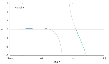
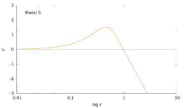
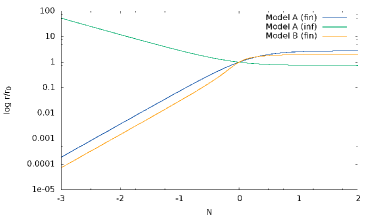
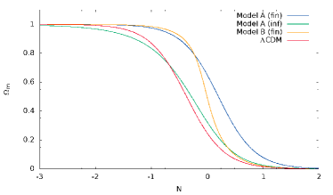
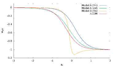
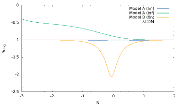
We chose two representative models to sketch a possible viable evolution of a bimetric gravity in Figures 1 and 2. The model A, described by , produces two viable branches. Although and evolve similarly in both branches, we find a phantom equation of state only in the finite one. An one-parameter model , such as model B with , is only able to produce a viable finite branch. Those models always produce a phantom since a positive expansion rate requires .
IV Comparing to Supernovae Ia Hubble diagram
To compare the background evolution of bimetric gravity models with observed SNe Ia, we use the SCP Union 2.1 Compilation Suzuki et al. (2012) containing 580 SNe Ia. For each observed SN Ia we can use the measured maximum magnitude in the B-band together with the stretch correction and the color correction to compute the likelihood for a bimetric model with
| (49) |
where and are nuisance parameters which weight the stretch- and color correction and denotes the absolute magnitude,
| (50) |
The marginalization over can be performed analytically, whereas we simplify the computation by using the values for and that minimize instead of computing the marginalization numerically. In addition, we add an intrinsic dispersion which we assume to be in order to obtain a for the best fit in a CDM cosmology.
We decided not to use other cosmological datasets like baryon acoustic oscillations because they are at the moment far weaker than SN Ia and CMB peak positions because their analysis depends on various assumptions which are not warranted in a non-standard model as the one we explore here. Nevertheless, our results are in agreement with Ref. Akrami et al. (2013b), where these additional datasets have been employed.
V Minimal models: 1-parameter models
It is very instructive to study in detail some simple subset among all the possible viable cosmologies. During our analysis we will mostly assume a vanishing explicit cosmological constant, i.e. (the only model with a non-vanishing cosmological constant that is studied in this work will be the 1-parameter model ). This subset of models is a very interesting one since those models may fit observational data without the need of a cosmological constant. In this section we assume moreover that all of the other vanish, except one, i.e. we restrict ourselves to models. In this case, as already shown, only one possibility, the model, turns out to be viable. In terms of simplicity, this is the minimal bimetric model, so it can help us gaining intuition on the behavior of this class of models. This model was already studied and compared to the SN Ia data in Akrami et al. (2013b); the same paper excludes the other models on the ground of their poor fit to data. The model is interesting also because can be easily solved analytically. Its evolution follows from Eq. (25),
| (51) |
Note that the evolution of does not depend on . In terms of the scale factor, the solution reads
| (52) |
To determine the constant , we use the background equation Eq. (15) at current time which provides and therefore
| (53) |
Depending on and , both a negative and positive is possible. To satisfy , we need to choose the positive sign in Eq. (52) if is positive, or the negative sign in case of a negative . The comparison with the SNIa Hubble diagram shows that has to be positive (see below).
With this result, the equation of state and are fully described through
| (54) | ||||
| (55) | ||||
| (56) |
Thus, in the viable minimal model, the equation of state always evolves from to . These equations imply a simple and testable relation between and valid at all times during matter domination:
| (57) |
In general, denoting with a subscript the present time, the following conditions must be satisfied by any model:
| (58) | ||||
| (59) |
(the last one is obtained from Eq. (20) after expressing the s in units of ). In particular, for the minimal model we obtain then a direct relation to the present value of the matter fractional density, which yields
| (60) |
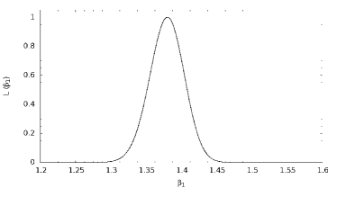
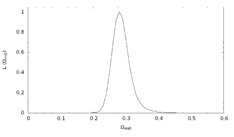
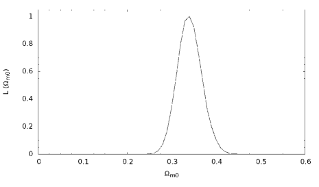
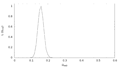
We fitted the model to the SN Union 2.1 catalog (see Figure 3) and obtained for the best fit. The most likely values for and are summarized in Table 1. We list also the present value of the equation of state expressed using the simple CPL parametrization Chevallier and Polarski (2001); Linder (2003)
| (61) |
in order to provide a quick comparison to present and future cosmological data.
The model is then a valid alternative to CDM in terms of simplicity, and although it does not reduce to CDM in any limit, it gives a good fit to the background data.
A second type of minimal models is described by identical couplings . As noted earlier, only those models with produce one viable finite branch. The evolution of , described by
| (62) |
has an analytical solution, though it is much more complicated than in a minimal model with only one non-vanishing coupling. However, the matter density parameter follows the simple relation
| (63) |
which, just like , is independent of . Of course, the present value is a function of . Again, we can use the set of equations (59) to obtain a relation between and ,
| (64) |
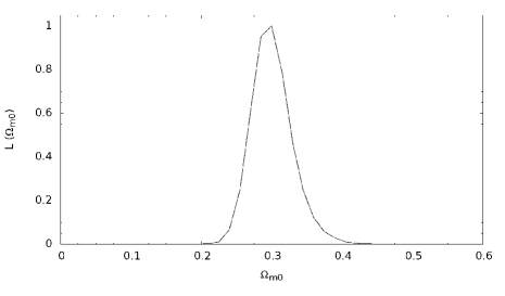
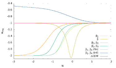
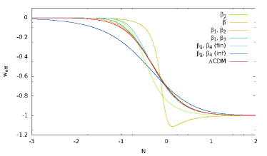
We found that both types of minimal models are only able to produce viable branches if the coupling parameters are positive and is located in a finite branch. Then Eq. (47) directly implies that all these minimal models are described by a phantom equation of state at any time. A comparison of both minimal models with observed SNe Ia yields the likelihoods in Figure 3 which provide the best fits listed in Table 1. Their equation of state is plotted in Figure 5.
| or | ||||||
|---|---|---|---|---|---|---|
VI Two-parameter models
We move now to models in which all vanish except two, taken in turn to be all possible combinations (we keep ). As already shown, we need to exclude all cases in which since we do not expect any viable models.
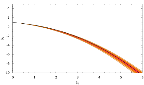
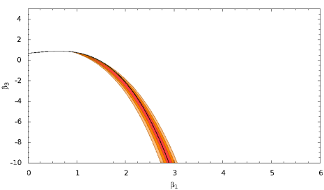
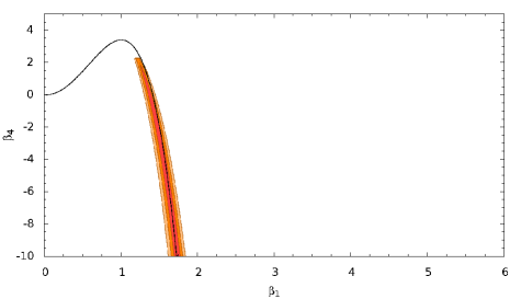
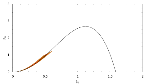
To compute the likelihood for , we divide the range in in bins of constant width and marginalize the likelihood over both -parameters with the restriction . Our results are summarized in Figure 4 where the left plots show the 68%, 95% and 99.7% confidence regions in the plane, the corresponding likelihoods for are illustrated in the right column. In all cases that are shown in Figure 4, we found bimetric gravity models which are consistent with observed SNe Ia. We always observe a strong degeneracy between the two free parameters, as already remarked in Ref. Akrami et al. (2013b).
As in the minimal cases, the system (59) gives a relation between pairs of and :
-
1.
For :
(65) -
2.
For :
(66) where the positive sign should be taken if and the negative one otherwise.
In all cases should be taken as the best fit value. The model does not have a simple analytic solution but the relation is easily solved numerically. These relation are plotted in the same Fig. 4; as one can see, they fit very well the degeneracy curves.
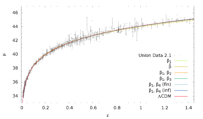
At , the relative error on the fitted , with (), are given in Table 4, where we determined the error by fitting the 68% contour with . For the best fit in all analyzed combinations, we show the evolution of the equation of state in Figure 5 and the distance moduli in comparison with the measured SNe Ia of the Union 2.1 Compilation in Figure 6.
Note that the analytic fit does not always need to correspond to a viable solution since it ignores the condition and in the finite and infinite branch, respectively. We therefore need to exclude some parameter regions. As an example, we analyze all models with positive and obtain
| (67) |
A necessary condition to satisfy the relation is
| (68) |
which excludes most of the models with . Similar boundaries of the coupling parameter corresponding to the highest order interaction exist in the and models, too.
Only the model is able to produces infinite branches. The likelihoods in Figure 4 for finite and infinite branches show that there is no parameter region in which the contours of both likelihoods overlap. If there is a model in which two viable branches co-exist, then at least one branch is strongly disfavored by SNe Ia observations.
| Model | |||
|---|---|---|---|
| CDM | 578.00 | ||
| 577.99 | |||
| 578.02 | |||
| 578.04 | |||
| (inf. branch ) | 578.60 |
VII conclusions
In this paper we studied a class of bimetric gravitational models that have been shown to be ghost-free and to induce cosmological acceleration. We define a viable cosmology as one in which the cosmic evolution broadly resembles the standard one, without bounces, singularities at finite time, and with a matter (or radiation) dominated past. Adopting spatially flat metrics we find that the system becomes effectively unidimensional and in some cases even analytical. This allows us to find a number of simple rules for viability which selects a subset of models and initial conditions. We show that if a branch is viable, then its final state is always deSitter. We also find the analytical condition for the occurrence of a phantom phase and we remark that observing a phantom crossing would rule out the entire class of viable bimetric models.
Then we show that among the models with only a single non-zero parameter, only one gives a viable cosmology, which well reproduces the SN data and can be taken as a simple, distinguishable alternative to CDM. The relation (57) provides a stringent test for this minimal model. For models with two coupling constants and without a cosmological constant, only three cases produce a viable cosmology. In several cases we find also an analytic expression for the background best fit which very closely approximates our numerical likelihood results.
These results allow to pre-select a number of cases for which a detailed study, including perturbation growth, can be performed. This task is carried out in a companion paper.
Acknowledgment
L.A. acknowledges support from DFG through the TRR33 project “The Dark Universe”. We are grateful to Y. Akrami, S. F. Hassan, S. Hoffmann, T. Koivisto, D. Mota, M. Sandstand, A. Schmidt-May, M. von Strauss for useful discussions. Special thanks to Valerio Marra for help with the supernovae data and to Mariele Motta for checking various equations. A.P. thanks the DAAD-WISE Fellowship for support.
References
- Akrami et al. [2013a] Y. Akrami, T. S. Koivisto, D. F. Mota, and M. Sandstad. Bimetric gravity doubly coupled to matter: theory and cosmological implications. JCAP, 10:046, October 2013a. doi: 10.1088/1475-7516/2013/10/046.
- Akrami et al. [2013b] Y. Akrami, T. S. Koivisto, and M. Sandstad. Accelerated expansion from ghost-free bigravity: a statistical analysis with improved generality. Journal of High Energy Physics, 3:99, March 2013b. doi: 10.1007/JHEP03(2013)099.
- Chevallier and Polarski [2001] M. Chevallier and D. Polarski. Accelerating Universes with Scaling Dark Matter. International Journal of Modern Physics D, 10:213–223, 2001. doi: 10.1142/S0218271801000822.
- Comelli et al. [2012] D. Comelli, M. Crisostomi, F. Nesti, and L. Pilo. FRW cosmology in ghost free massive gravity from bigravity. Journal of High Energy Physics, 3:67, March 2012. doi: 10.1007/JHEP03(2012)067.
- Comelli et al. [2012] D. Comelli, M. Crisostomi, and L. Pilo. Perturbations in Massive Gravity Cosmology. JHEP, 1206:085, 2012. doi: 10.1007/JHEP06(2012)085.
- De Felice et al. [2013] A. De Felice, T. Nakamura, and T. Tanaka. Possible existence of viable models of bi-gravity with detectable graviton oscillations by gravitational wave detectors. ArXiv e-prints, April 2013.
- de Rham et al. [2011] C. de Rham, G. Gabadadze, and A. J. Tolley. Resummation of Massive Gravity. Physical Review Letters, 106(23):231101, June 2011. doi: 10.1103/PhysRevLett.106.231101.
- Deffayet et al. [2011] C. Deffayet, Xian Gao, D.A. Steer, and G. Zahariade. From k-essence to generalised Galileons. Phys.Rev., D84:064039, 2011.
- Deser et al. [2013] S. Deser, M. Sandora, and A. Waldron. No consistent bimetric gravity? Phys. Rev. D, 88(8):081501, October 2013. doi: 10.1103/PhysRevD.88.081501.
- Hassan and Rosen [2012a] S. F. Hassan and R. A. Rosen. Bimetric gravity from ghost-free massive gravity. Journal of High Energy Physics, 2:126, February 2012a. doi: 10.1007/JHEP02(2012)126.
- Hassan and Rosen [2012b] S. F. Hassan and R. A. Rosen. Resolving the Ghost Problem in Nonlinear Massive Gravity. Physical Review Letters, 108(4):041101, January 2012b. doi: 10.1103/PhysRevLett.108.041101.
- Hassan et al. [2012] S. F. Hassan, R. A. Rosen, and A. Schmidt-May. Ghost-free massive gravity with a general reference metric. Journal of High Energy Physics, 2:26, February 2012. doi: 10.1007/JHEP02(2012)026.
- Hassan et al. [2013a] S. F. Hassan, A. Schmidt-May, and M. von Strauss. On partially massless bimetric gravity. Physics Letters B, 726:834–838, November 2013a. doi: 10.1016/j.physletb.2013.09.021.
- Hassan et al. [2013b] S. F. Hassan, A. Schmidt-May, and M. von Strauss. Higher Derivative Gravity and Conformal Gravity From Bimetric and Partially Massless Bimetric Theory. ArXiv e-prints, March 2013b.
- Hinterbichler [2012] K. Hinterbichler. Theoretical aspects of massive gravity. Reviews of Modern Physics, 84:671–710, April 2012. doi: 10.1103/RevModPhys.84.671.
- Horndeski [1974] Gregory Walter Horndeski. Second-order scalar-tensor field equations in a four-dimensional space. Int.J.Th.Phys., 10:363–384, 1974.
- Linder [2003] E. V. Linder. Exploring the Expansion History of the Universe. Physical Review Letters, 90(9):091301, March 2003. doi: 10.1103/PhysRevLett.90.091301.
- Suzuki et al. [2012] N. Suzuki, D. Rubin, C. Lidman, G. Aldering, R. Amanullah, et al. The Hubble Space Telescope Cluster Supernova Survey: V. Improving the Dark Energy Constraints Above z=1 and Building an Early-Type-Hosted Supernova Sample. Astrophys.J., 746:85, 2012.
- Volkov [2012] M. S. Volkov. Cosmological solutions with massive gravitons in the bigravity theory. Journal of High Energy Physics, 1:35, January 2012. doi: 10.1007/JHEP01(2012)035.
- von Strauss et al. [2012] Mikael von Strauss, Angnis Schmidt-May, Jonas Enander, Edvard Mörtsell, and S.F. Hassan. Cosmological solutions in bimetric gravity and their observational tests. Journal of Cosmology and Astroparticle Physics, 2012(03):042, 2012. URL http://stacks.iop.org/1475-7516/2012/i=03/a=042.