Abstract

The dominance of type-II seesaw mechanism for neutrino masses has attracted considerable attention because of a number of advantages. We show a novel approach to achieve Type-II seesaw dominance in non-supersymmetric $SO(10)$ grand unification where a low mass $Z^{\prime}$ boson and specific patterns of right-handed neutrino masses are predicted within the accessible energy range of the Large Hadron Collider. In spite of the high value of the seesaw scale, $M_{\Delta_{L}}\simeq 10^{8}-10^{9}$ GeV, the model predicts new dominant contributions to neutrino-less double beta decay in the $W_{L}-W_{L}$ channel close to the current experimental limits via exchanges of heavier singlet fermions used as essential ingredients of this model even when the light active neutrino masses are normally hierarchical or invertedly hierarchical. We obtain upper bounds on the lightest sterile neutrino mass $m_{s}\lesssim 3.0$ GeV, $2.0$ GeV, and $0.7$ GeV for normally hierarchical, invertedly hierarchical and quasi-degenerate patterns of light neutrino masses, respectively. The underlying non-unitarity effects lead to lepton flavor violating decay branching ratios within the reach of ongoing or planned experiments and the leptonic CP-violation parameter nearly two order larger than the quark sector. Some of the predicted values on proton lifetime for $p\to e^{+}\pi^{0}$ are found to be within the currently accessible search limits. Other aspects of model applications including leptogenesis etc. are briefly indicated.

New mechanism for Type-II seesaw dominance in SO(10) with low-mass $Z^{\prime}$, RH neutrinos, and verifiable LFV, LNV and proton decay

Bidyut Prava Nayak ^† and M. K. Parida ^∗

Centre of Excellence in Theoretical and Mathematical  Sciences
SOA University, Khandagiri Square, Bhubaneswar 751030, India
^∗email:parida.minaketan@gmail.com
^†email:bidyutprava25@gmail.com

1 INTRODUCTION

Experimental evidences on tiny neutrino masses and their large mixings have attracted considerable attention as physics beyond the standard model (SM) leading to different mechanisms for neutrino mass generation. Most of these models are based upon the underlying assumption that neutrinos are Majorana fermions that may manifest in the detection of events in neutrino-less double beta ($0\nu\beta\beta$) decay experiments on which a number of investigations are in progress [1, 2, 3]. Theories of neutrino masses and mixings are placed on a much stronger footing if they originate from left-right symmetric (LRS) [8, 9] grand unified theories such as SO(10) where, besides grand unification of three forces of nature, P ($=$Parity) and CP-violations have spontaneous-breaking origins, the fermion masses of all the three generations are adequately fitted [10], all the $15$ fermions plus the right-handed neutrino ($N$) are unified into a single spinorial representation ${\bf 16}$ and the canonical ($\equiv$ type-I ) seesaw formula for neutrino masses is predicted by the theory. More recently non-SUSY $SO(10)$ origin of cold dark matter has been also suggested [11]. Although type-I seesaw formula was also proposed by using extensions of the SM [5, 6], it is well known that this was advanced even much before the atmospheric neutrino oscillation data [7] and it is interesting to note that Gell-Mann, Ramond and Slansky had used the left-right symmetric SO(10) theory and its Higgs representations ${10}_{H},{126}_{H}$ to derive it. A special feature of left-right (LR) gauge theories and SO(10) grand unification is that the canonical seesaw formula for neutrino masses is always accompanied by type-II seesaw formula [13] for Majorana neutrino mass matrix

$$\mathcal{M_{\nu}}=m^{II}_{\nu}+m^{I}_{\nu},\\$$ (1)

$$m^{I}_{\nu}=-M_{D}\frac{1}{M_{N}}M_{D}^{T},$$ (2)

$$m^{II}_{\nu}=fv_{L}$$ (3)

where $M_{D}(M_{N})$ is Dirac (RH-Majorana) neutrino mass, $v_{L}$ is the induced vacuum expectation value (VEV) of the left-handed (LH) triplet $\Delta_{L}$, and $f$ is the Yukawa coupling of the triplet. Normally, because of the underlying quark-lepton symmetry in SO(10), $M_{D}$ is of the same order as $M_{u}$, the up-quark mass matrix. Then the neutrino oscillation data forces the canonical seesaw scale to be large, $M_{N}\geq 10^{11}$ GeV. Similarly the type-II seesaw scale is also large. With such high seesaw scales, these two mechanisms in SO(10) can not be directly verified at low energies or by the Large Hadron Collider (LHC) except for the indirect signature through the light active neutrino mediated $0\nu\beta\beta$ decay, and possibly leptogenesis.
It is well known that the theoretical predictions of branching ratios for LFV decays such as $\mu\to e\gamma$, $\tau\to\mu\gamma$, $\tau\to e\gamma$, and $\mu\to e{\bar{e}}e$ closer to their experimental limits are generic features of SUSY GUTs even with high seesaw scales but, in non-SUSY models with such seesaw scales, they are far below the experimental limits. Recently they have been also predicted to be experimentally accessible along with low-mass $W_{R},Z_{R}$ bosons through TeV scale gauged inverse seesaw mechanism [14] in SUSY SO(10). In the absence of any evidence of supersymmetry so far, alternative non-SUSY SO(10) models have been found with predictions of substantial LFV decays and TeV scale $Z^{\prime}$ bosons. Although two-step breakings of LR gauge theory was embedded earlier in non-SUSY GUTs with low-mass $Z^{\prime}$ [16], its successful compliance with neutrino oscillation data has been possible in the context of inverse seesaw mechanism and predictions of LFV decays [17], or with the predictions of low-mass $W_{R},Z_{R}$ bosons, LFV decays, observable neutron oscillations, and dominant LNV decay via extended seesaw mechanism [18]. Possibility of LHC accessible low-mass $Z^{\prime}$ has been also investigated recently in the context of heterotic string models [19]. Another attractive aspect of non-SUSY SO(10) is rare kaon decay and neutron-antineutron oscillation which has been discussed in a recent work with inverse seesaw mechanism for light neutrino masses and TeV scale $Z^{\prime}$ bosons but having much larger $W_{R}$ mass not accessible to LHC [20]. The viability of the model of ref.[14] depends on the discovery of TeV scale SUSY , TeV scale $W_{R},Z_{R}$ bosons, and TeV scale pseudo-Dirac neutrinos. The viability of the non-SUSY model of ref.[17] depends on the discovery of TeV scale low-mass $Z_{R}$ boson and heavy pseudo Dirac neutrinos in the range $100-1200$ GeV; both types of models predict proton lifetime within the Super-K search limit. The falsifiability of the non-SUSY model of ref.[20] depends upon any one of the following predicted observables: TeV scale $Z_{R}$ boson, dominant neutrino-less double beta decay, heavy Majorana type sterile and right-handed neutrinos, neutron oscillation, and rare kaon decays. Whereas the neutrino mass generation mechanism in all these models is through gauged inverse seesaw mechanism, our main thrust in the present work is type-II seesaw. A key ansatz to resolve the issue of large mixing in the neutrino sector and small mixing in the quark sector has been suggested to be through type-II seesaw dominance [21] via renormalisation group evolution of quasi-degenerate neutrino masses that holds in supersymmetric quark-lepton unified theories [8] or SO(10) and for large values of $\tan\beta$ which represents the ratio of vacuum expectation values (VEVs) of up-type and down type Higgs doublets. In an interesting approach to understand neutrino mixing in SUSY theories, it has been shown [22] that the maximality of atmospheric neutrino mixing is an automatic cosnsequence of type-II seesaw dominance and $b-\tau$ unification that does not require quasi-degeneracy of the associated neutrino masses. A number of consequences of this approach have been explored to explain all the fermion masses and mixings by utilising type-II seesaw, or a combination of both type-I and type-II seesaw [23, 24] through SUSY SO(10). As a further interesting property of type-II seesaw dominance, it has been recently shown [25] without using any flavor symmetry that the well known tri-bimaximal mixing pattern for neutrino mixings is simply a consequence of rotation in the flavor space. Although several models of Type-II seesaw dominance in SUSY SO(10) have been investigated, precision gauge coupling unification is distorted in most cases. All the charged fermion mass fittings in the conventional one-step breaking of SUSY GUTs including fits to the neutrino oscillation data require the left-handed triplet to be lighter than the type-I seesaw scale. The gauge coupling evolutions being sensitive to the quantum numbers of the LH triplet $\Delta_{L}(3,-2,1)$ under SM gauge group, tend to misalign the precision unification in the minimal scenario achieved without the lighter triplet.
Two kinds of SO(10) models have been suggested for ensuring precision gauge coupling unification in the presence of type-II seesaw dominance. In the first type of SUSY model [26], SO(10) breaks at a very high scale $M_{U}\geq 10^{17}$ GeV to SUSY SU(5) which further breaks to the minimal supersymmeric standard model (MSSM) at the usual SUSY GUT scale $M_{U}\sim 2\times 10^{16}$ GeV. Type-II seesaw dominance is achieved by fine tuning the mass of the full $SU(5)$ multiplet ${15}_{H}$ containing the $\Delta_{L}(3,-2,1)$ to remain at the desired type-II scale $M_{\Delta_{L}}=10^{11}-10^{13}$ GeV. Since the full multiplet ${15}_{H}$ is at the intermediate scale, although the evolutions of the three gauge couplings of the MSSM gauge group deflect from their original paths for $\mu>M_{\Delta_{L}}$, they converge exactly at the same scale $M_{U}$ as the MSSM unification scale but with a slightly larger value of the GUT coupling leading to a marginal reduction of proton-lifetime prediction compared to SUSY SU(5). In the second class of models applicable to a non-SUSY or split-SUSY case [27], the grand unification group SO(10) breaks directly to the SM gauge symmetry at the GUT-scale $M_{U}\sim 2\times 10^{16}$ GeV and by tuning the full SU(5) scalar multiplet ${15}_{H}$ to have degenerate masses at $M_{\Delta_{L}}=10^{11}-10^{13}$ GeV, the type-II seesaw dominance is achieved. The question of precision unification is answered in this model by pulling out all the super-partner scalar components of the MSSM but by keeping all the fermionic superpartners and the two Higgs doublets near the TeV scale. In the non-SUSY case the TeV scale fermions can be also equivalently replaced by complex scalars carrying the same quantum numbers. The proton lifetime prediction is $\tau_{P}(p\to e^{+}\pi^{0})\simeq 10^{35}$ Yrs. in this model.
In the context of LR gauge theory, type-II seesaw mechanism was originally proposed with manifest left right symmetric gauge group $SU(2)_{L}\times SU(2)_{R}\times U(1)_{B-L}\times SU(3)_{C}\times D$ ($g_{2L}=g_{2R}$) ($\equiv G_{2213D}$) where both the left- and the right-handed triplets are allowed to have the same mass scale as the LR symmetry breaking (or the Parity breaking ) scale [12]. With the emergence of D-Parity and its breaking leading to decoupling of Parity and $SU(2)_{R}$ breakings [28], a new class of asymmetric LR gauge group also emerged: $SU(2)_{L}\times SU(2)_{R}\times U(1)_{B-L}\times SU(3)_{C}$ ($g_{2L}\neq g_{2R}$) ($\equiv G_{2213}$) where the left-handed triplet acquired larger mass than the RH triplet leading to the type-I seesaw dominance and suppression of type-II seesaw in $SO(10)$ [30]. It is possible to accommodate both types of intermediate symmetries in non-SUSY SO(10) but these models make negligible predictions for branching ratios of charged LFV processes and they leave no other experimental signatures to be verifiable at low or LHC energies except $0\nu\beta\beta$ decay.
The purpose of this work is to show that in a class of models descending from non-SUSY SO(10) or from Pati-Salam gauge symmetrty, type-II seesaw dominance at intermediate scales ($M_{\Delta}\simeq 10^{8}-10^{9}$ GeV) but with $M_{N}\sim O(1)-O(10)$ TeV can be realised by cancellation of the type-I seesaw contribution along with the prediction of a $Z^{\prime}$ boson at $\sim O(1)-O(10)$ TeV scale accessible to the large Hadron Collider (LHC) where $U(1)_{R}\times U(1)_{B-L}$ breaks spontaneously to $U(1)_{Y}$ through the VEV of the RH triplet component of Higgs scalar contained in ${126}_{H}$ that carries $B-L=-2$.

Although two-step breakings of LR gauge theory was embedded earlier in non-SUSY GUTs with low-mass $Z^{\prime}$ [16], its successful compliance with neutrino oscillation data has been possible in the context of inverse seesaw mechanism [17].

We also discuss how the type-II seesaw contribution dominates over the linear seesaw formula. Whereas in all previous Type-II seesaw dominance models in SO(10), the RH Majorana neutrino masses have been very large and inaccessible for accelerator energies, the present model predicts these masses in the LHC accessible range. In spite of large values of the $W_{R}$ boson and the doubly charged Higgs boson $\Delta_{L}^{++},\Delta_{R}^{++}$ masses, it is quite interesting to note that the model predicts a new observable contribution to $0\nu\beta\beta$ decay in the $W_{L}-W_{L}$ channel. The key ingredients to achieve type-II seesaw dominance by complete suppression of type-I seesaw contribution are addition of one SO(10) singlet fermion per generation ($S_{i},i=1,2,3$) and utilization of the additional Higgs representation ${16}_{H}$ to generate the $N-S$ mixing term in the Lagrangian through Higgs-Yukawa interaction. The underlying leptonic non-unitarity effects lead to substantial LFV decay branching ratios and leptonic CP-violation accessible to ongoing search experiments. We derive a new formula for the half-life of $0\nu\beta\beta$ decay as a function of the fermion singlet masses and extract lower bound on the lightest sterile neutrino mass from the existing experimental lower bounds on the half-life of different experimental groups. For certain regions of parameter space of the model, we also find the proton lifetime for $p\to e^{+}\pi^{0}$ to be accessible to ongoing or planned experiments.
Compared to earlier existing SO(10) based type-II seesaw dominant models whose RH neutrino masses are in the inaccessible range and new gauge bosons are in the mass range $10^{15}-10^{17}$ GeV, the present model predictions on LHC scale $Z^{\prime}$, light and heavy Majorana type sterile neutrinos, RH Majorana neutrino masses in the range $\simeq{100-10000}$ GeV accessible to LHC in the $W_{L}-W_{L}$ channel through dilepton production, the LFV branching ratios closer to experimental limits, and dominant $0\nu\beta\beta$ decay amplitudes caused by sterile neutrino exchanges provide a rich testing ground for new physics signatures.
This paper is organized as follows. In Sec.2. we give an outline of the model and discuss gauge coupling unification along with proton lifetime predictions. In Sec.3 we derive type-II seesaw dominance formula and show how the model predicts RH neutrino masses from fits to the neutrino oscillation data. In Sec.4 we discuss the derivation of Dirac neutrino mass matrix from the GUT scale fit to fermion masses. In Sec.5 we discuss predictions on lepton flavor violation and leptonic CP violation due to the underlying non-unitarity effects. In Sec.6 we discuss briefly analytic derivation of amplitudes on lepton number violation. In Sec.7 we discuss predictions on effective mass parameters and half life for $0\nu\beta\beta$ where we also obtain the singlet fermion mass bounds. We also indicate very briefly some plausible model applications including effects on electroweak precision observables, $Z-Z^{\prime}$ mixings, dilepton production, and leptogenesis in Sec.8. We summarize and conclude our results in Sec.9.

2 UNIFICATION WITH TeV SCALE $Z^{\prime}$

In this section we devise two symmetry breaking chains of non-SUSY $SO(10)$ theory, one with LR symmetric gauge theory with unbroken D-Parity and another without D-Parity at the intermediate scale. In the subsequent sections we will compare the ability of the two models to accommodate type-II seesaw dominance to distinguish one model from the other. As necessary requirements, we introduce one $SO(10)$-singlet per generation ($S_{i},i=1,2,3$) and Higgs representations ${126}_{H}$ and ${16}_{H}$ in both the models .

2.1 Models from $SO(10)$ symmetry breaking

Different steps of symmetry breaking is given below for the following two models:

Model-I

$$SO(10) \stackrel{{\scriptstyle(M_{U}=M_{P})}}{{\longrightarrow}} SU(2)_{L}\times SU(2)_{R}\times U(1)_{B-L}\times SU(3)_{C}~{}~{}[G_{2213}]$$

$$\stackrel{{\scriptstyle(M_{R}^{+})}}{{\longrightarrow}} SU(2)_{L}\times U(1)_{R}\times U(1)_{B-L}\times SU(3)_{C}~{}~{}[G_{2113}]$$

$$\stackrel{{\scriptstyle(M_{R}^{0})}}{{\longrightarrow}} SU(2)_{L}\times U(1)_{Y}\times SU(3)_{C}~{}~{}[\rm SM]$$

$$\stackrel{{\scriptstyle(M_{Z})}}{{\longrightarrow}} SU(3)_{C}\times U(1)_{Q},$$

Model-II

$$SO(10) \stackrel{{\scriptstyle(M_{U})}}{{\longrightarrow}} SU(2)_{L}\times SU(2)_{R}\times U(1)_{B-L}\times SU(3)_{C}[G_{2213D}]$$

$$\stackrel{{\scriptstyle(M_{R}^{+}=M_{P})}}{{\longrightarrow}} SU(2)_{L}\times U(1)_{R}\times U(1)_{B-L}\times SU(3)_{C}~{}~{}[G_{2113}]$$

$$\stackrel{{\scriptstyle(M_{R}^{0})}}{{\longrightarrow}} SU(2)_{L}\times U(1)_{Y}\times SU(3)_{C}~{}~{}[\rm SM]$$

$$\stackrel{{\scriptstyle(M_{Z})}}{{\longrightarrow}} SU(3)_{C}\times U(1)_{Q}.$$

In Model-II, $SU(2)_{L}\times SU(2)_{R}\times U(1)_{B-L}\times SU(3)_{C}\times D~{}~{}[\equiv G_{2213D}](g_{2L}=g_{2R})$ is obtained by breaking the GUT-symmetry and by giving vacuum expectation value (VEV) to the D-Parity even singlet $(1,1,0,1)\subset(1,1,15)\subset{210}_{H}$ [28, 29] where the first, second, and the third set of quantum numbers of the scalar components are under $G_{2213P}$, the Pati-Salam symmetry $G_{224}$, and $SO(10)$, respectively. As a result, the Higgs sector is symmetric below $\mu=M_{U}$ leading to equality between the gauge couplings $g_{2L}(M_{R}^{+})$ and $g_{2R}(M_{R}^{+})$ . In this case the LR discrete symmetry ($\equiv$ Parity) survives down to the intermediate scale ,$M_{R^{+}}=M_{P}$. The second step of symmetry breaking is implemented by assigning VEV to the neutral component of the right-handed (RH) Higgs triplet $\sigma_{R}(1,3,0,1)\subset{45}_{H}$ that carries $B-L=0$. The third step of breaking to SM is carried out by assigning VEV of ${\mathcal{O}}(5-10)$ TeV to the $G_{2113}$ component $\Delta^{0}_{R}(1,1,-2,1)$ contained in the RH triplet $\Delta_{R}(1,3,-2,1)\subset{126}_{H}$ carrying $B-L=-2$. This is responsible for RH Majorana neutrino mass generation $M_{N}=fV_{R}$ where $V_{R}=\langle\Delta_{R}^{0}\rangle$ and $f$ is the Yukawa coupling of ${126}^{\dagger}$ to $SO(10)$ spinorial fermionic representation :$f{\bf 16.16.126^{\dagger}_{H}}$. We introduce $SO(10)$ invariant $N-S$ mixing mass via the Yukawa interaction $y_{\chi}{\bf 16.1.16_{H}^{\dagger}}$ and obtain the mixing mass $M=y_{\chi}V_{\chi}$ where $V_{\chi}=\langle\chi_{R}^{0}\rangle$ by noting that under $G_{2113}$ the submultiplet $\chi_{R}^{0}(1,1/2,-1,1)$ is contained in the $G_{2213}$ doublet $\chi_{R}(1,2,-1,1)\subset 16_{H}$. The symmetry breaking in the last step is implemented through the SM Higgs doublet contained in the bidoublet $\phi(2,2,0,1)\subset{10}_{H}$ of SO(10). This is the minimal Higgs structure of the model, although we will utilise two different Higgs doublets $\phi_{u}\subset 10_{H_{1}}$ and $\phi_{d}\subset 10_{H_{2}}$ for fermion mass fits. In Model-I, the GUT symmetry breaks to LR gauge symmetry $G_{2213}(g_{2L}\neq g_{2R})$ in such a way that the D-parity breaks at the GUT scale and is decoupled from $SU(2)_{R}$ breaking that occurs at the intermediate scale. This is achieved by giving GUT scale VEV to the D-parity odd singlet-scalar component in $(1,1,0,1)_{H}\subset(1,1,15)_{H}\subset{45}_{H}$ where the first, second , and third submultiplets are under $G_{2213}$, the Pati-Salam symmetry $G_{224}$, and $SO(10)$, respectively. In this case by adopting the D-Parity breaking mechanism [28] in $SO(10)$, normally the LH triplet component $\Delta_{L}(3,1,-2,1)\subset{126}_{H}$ and the LH doublet component $\chi_{L}(2,1,-1,1)\subset{16}_{H}$ acquire masses at the GUT scale while the RH triplet and RH doublet components, $\Delta_{R}(1,3,-2,1)\subset{126}_{H}$ $\chi_{R}(1,2,-1,1)\subset{16}_{H}$, can be made much lighter. We have noted that in the presence of color octet at lower scales, found to be necessary in this Model-I as well as in Model-II, precision gauge coupling is achieved even if the the parameters of the Higgs potential are tuned so as to have the LH triplet mass at intermediate scale, $M_{\Delta_{L}}\simeq 10^{8}-10^{9}$  GeV. The presence of $\Delta_{L}(3,1,-2,1)$ at the intermediate scale plays a crucial role in achieving Type-II seesaw dominance as would be explained in the following section. The necessary presence of lighter LH triplets in GUTs with or without vanishing $B-L$ value for physically appealing predictions was pointed out earlier in achieving observable matter anti-matter oscillations [31], in the context of low-scale leptogenesis [32], and type-II seesaw dominance in SUSY, non-SUSY and split-SUSY models [26, 27], and also for TeV scale LR gauge theory originating from SUSY $SO(10)$ grand unification[14].

2.2 Renormalization group solutions to mass scales

In this section while safeguarding precise unification of gauge couplings at the GUT scale, we discuss allowed solutions of renormalization group equations (RGEs) for the mass scales $M_{U},M_{R^{+}}$, and $M_{R^{0}}$ as a function of the mass $M_{C}$ of the lighter color octet $C_{8}(1,1,0,8)\subset{45}_{H}$. The Higgs scalars contributing to RG evolutions are presented in Table 1 for Model I. In Model II, in addition to the Higgs scalars shown in Table 1, the masses of the left handed scalars $\chi_{L}(2,1,-1,1)$ and $\sigma_{L}(3,1,0,1)$ are naturally constrained to be at $\mu=M_{R}^{+}=M_{P}=$ the parity violation scale.

Higgs scalars

Mass scale $(\mu)$	Symmetry	Higgs scalars (Model-I)
$M_{Z}-M_{R}^{0}$	$G_{213}$	$\Phi(2,1,1)$
$M_{R}^{0}-M_{R}^{+}$	$G_{2113}$	${\small\begin{array}[]{l}\Phi_{1}(2,1,0,1),\Phi_{2}(2,1,0,1),\\[5.69054pt] \chi_{R}(1,1/2,-1,1),\Delta_{R}(1,1,-2,1),\\[5.69054pt] C_{8}(1,0,0,8)\end{array}}$
$M_{R}^{+}-M_{U}$	$G_{2213}$	${\small\begin{array}[]{l}\Phi_{1}(2,2,0,1),\Phi_{2}(2,2,0,1)),\\[5.69054pt] \chi_{R}(1,2,-1,1),\Delta_{R}(1,3,-2,1),\\[5.69054pt] \Delta_{L}(3,1,-2,1),C_{8}(1,0,0,8),\\[5.69054pt] \sigma_{R}(1,3,0,1)\end{array}}$

Table 1: Higgs scalars and their quantum numbers used in Model-I in the respective ranges of mass scales. The mass of colour octet $C_{8}(1,0,0,8)$ has been used in the range $10^{4}-10^{11}$ GeV contributing to the variation of predicted proton lifetime discussed below in Sec.2.3. In Model-II, in addition to these scalars, the masses of left handed scalars $\chi_{L}(2,1,-1,1)$ and $\sigma_{L}(3,1,0,1)$ are constrained to be at $\mu=M_{R}^{+}=M_{P}=$ the parity violation scale.

The renormalisation group (RG) coefficients for the minimal cases have been given in Appendix A to which those due to the color octet scalar in both models and the LH triplet $\Delta_{L}$ in Model-I in their suitable ranges of the running scale have been added.

Model-I:
As shown in Table 2 for Model-I, with $M_{\Delta_{L}}=10^{8}$ GeV the $G_{2213}$ symmetry is found to survive down to $M_{R^{+}}=(10^{8}-10^{10})$ GeV with larger or smaller unification scale depending upon the color octet mass. In particular we note one set of solutions,

$$M_{R^{0}} = 10~{}{\rm TeV},~{}M_{R^{+}}=10^{9.7}{\rm GeV},~{}M_{U}=10^{15.62}{\rm GeV},$$

$$M_{\Delta_{L}} = 10^{8}~{}{\rm GeV},~{}M_{C}=10^{10.9}{\rm GeV}.$$ (4)

As explained in the following sections, this set of solutions are found to be attractive both from the prospects of achieving type-II seesaw dominance and detecting proton decay at Hyper-Kamiokande. with $M_{U}=6.5\times 10^{15}$ GeV when the color octet mass is at $M_{C}\sim 10^{11}$ GeV. As discussed below the proton lifetime in this case is closer to the current experimental limit. With allowed values of $M_{R^{0}}=(5-10)$ TeV, this model also predicts $M_{Z^{\prime}}\simeq(1.2-3.5)$ TeV in the accessible range of the Large Hadron Collider. As discussed in the following Sec.3, because of the low mass of the $Z^{\prime}$ boson associated with TeV scale VEV of $V_{R}$, the type-II seesaw mechanism predicts RH neutrino masses which can be testified at the LHC or future high energy accelerators.

$M_{R}^{0}$	$M_{C}$	$M^{+}_{R}$	$M_{G}$	$\alpha_{G}^{-1}$	$\tau_{p}$
(TeV)	(GeV)	(GeV)	(GeV)		(Yrs.)
10	$10^{4.5}$	$10^{9}$	$10^{16.9}$	41.1	$5.4\times 10^{39}$
10	$10^{5}$	$10^{8.9}$	$10^{16.74}$	41.4	$1.1\times 10^{39}$
10	$10^{7}$	$10^{9}$	$10^{16.4}$	41.7	$8.4\times 10^{37}$
10	$10^{10.9}$	$10^{9.7}$	$10^{15.63}$	41.9	$3.2\times 10^{34}$
5	$10^{7.8}$	$10^{8.8}$	$10^{16.4}$	41.5	$9\times 10^{37}$

Table 2: Allowed values of mass scales as solutions of RGEs for gauge couplings for Model-I with fixed value of the LH triplet mass $M_{\Delta}=10^{8}$  GeV,

The RG evolution of gauge couplings for the set of mass scales given in eq.(4) is presented in Fig.1 showing clearly the unification of the four gauge couplings of the $G_{2213}$ intermediate gauge symmetry.

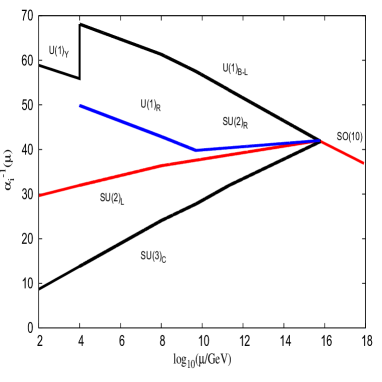
Figure 1: Two loop gauge coupling unification in the $SO(10)$ symmetry breaking chain with $M_{U}=10^{15.62}$ GeV and $M^{+}_{R}=10^{9.7}$, $M_{\Delta_{L}}=10^{8}$GeV with a low mass $Z^{\prime}$ boson at $M_{R}^{0}=10$ TeV for Model-I.

Model-II:
In addition to the Higgs scalars of Table 1, this model has the masses of left handed scalars $\chi_{L}(2,1,-1,1)$ and $\sigma_{L}(3,1,0,1)$ naturally at $\mu=M_{R}^{+}=M_{P}=$ the parity violation scale. As shown in Table 3 for Model-II, the $G_{2213D}$ symmetry is found to survive down to $M_{R^{+}}=M_{P}=10^{8.2}$ GeV with $M_{U}=6.5\times 10^{15}$ GeV when the color octet mass is at $M_{C}=10^{8}$ GeV. As discussed below, the proton lifetime in this case is closer to the current experimental limit.

$M_{R}^{0}$	$M_{C}$	$M^{+}_{R}$	$M_{G}$	$\alpha_{G}^{-1}$	$\tau_{p}$
(TeV)	(GeV)	(GeV)	(GeV)		(Yrs.)
10	$10^{4.5}$	$10^{7.886}$	$10^{16.15}$	40.25	$4.3\times 10^{36}$
10	$10^{5.5}$	$10^{7.89}$	$10^{16.04}$	40.64	$1.6\times 10^{36}$
10	$10^{8}$	$10^{8.789}$	$10^{15.62}$	41.49	$3.9\times 10^{34}$
10	$10^{8.5}$	$10^{8.8}$	$10^{15.5}$	41.69	$1.12\times 10^{34}$
5	$10^{5.8}$	$10^{7.2}$	$10^{15.83}$	41.15	$2.3\times 10^{35}$

Table 3: Allowed mass scales as solutions of renormalisation group equations for Model-II as described in the text.

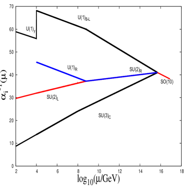
Figure 2: Two loop gauge coupling unification in the $SO(10)$ symmetry breaking chain with $M_{U}=10^{15.62}$ GeV and $M_{R^{+}}=10^{8.7}$ GeV with a low mass $Z^{\prime}$ boson at $M_{R}^{0}=10$ TeV for Model-II.

One example of RG evolution of gauge couplings is shown in Fig.2 for $M_{R^{0}}=10$ GeV, $M_{R^{+}}=10^{8.7}$ GeV, $M_{C}=10^{8}$ GeV, and $M_{U}=6.5\times 10^{15}$ GeV. Clearly the figure shows precise unification of the three gauge couplings of the intermediate gauge symmetry $G_{2213P}$ at the GUT scale. For all other solutions given in Table-I, the RG evolutions and unification of gauge couplings are similar. In both the models, with allowed values of $M_{R^{+}}\gg M_{R^{0}}=5-10$ TeV, the numerical values of gauge couplings $g_{2L},g_{1R}$ and $g_{B-L}$ predict [33],

$$M_{Z^{\prime}}=(1.2-3.5){\rm TeV}.$$ (5)

2.3 Proton lifetime prediction

In this section we discuss predictions on proton lifetimes in the two models and compare them with the current Super-Kamiokande limit and reachable limits by future experiments such as the Hyper-Kamiokande [34]. Currently, the Super-Kamiokande detector has reached the search limit

$${(\tau_{p})}_{expt.}(p\to e^{+}\pi^{0}) \geq 1.4\times 10^{34}~{}~{}{\rm yrs},$$ (6)

The proposed $5.6$ Megaton years Cherenkov water detector at Hyper-Kamiokande is expected to probe into lifetime [34],

$${(\tau_{p})}_{Hyper-K.}(p\to e^{+}\pi^{0}) \geq 1.3\times 10^{35}~{}~{}{\rm yrs},$$ (7)

The width of the proton decay for $p\to e^{+}\pi^{0}$ is expressed as [35]

$$\Gamma(p\rightarrow e^{+}\pi^{0}) = \left(\frac{m_{p}}{64\pi f_{\pi}^{2}}\right)\times\left(\frac{{g_{G}}^{4}}{{M_{U}}^{4}}\right)$$ (8)

$$|A_{L}|^{2}|\bar{\alpha_{H}}|^{2}(1+D+F)^{2}\times R.$$

where $R=[(A_{SR}^{2}+A_{SL}^{2})(1+|{V_{ud}}|^{2})^{2}]$ for $SO(10)$, $V_{ud}=0.974=$ the $(1,1)$ element of $V_{CKM}$ for quark mixings, $A_{SL}(A_{SR})$ is the short-distance renormalisation factor in the left (right) sectors and $A_{L}=1.25=$ long distance renormalization factor. $M_{U}=$ degenerate mass of $24$ superheavy gauge bosons in $SO(10)$, $\bar{\alpha}_{H}=$ hadronic matrix element, $m_{p}=$ proton mass $=938.3$ MeV, $f_{\pi}=$ pion decay constant $=139$ MeV, and the chiral Lagrangian parameters are $D=0.81$ and $F=0.47$. With $\alpha_{H}=\bar{\alpha_{H}}(1+D+F)=0.012$ GeV³ obtained from lattice gauge theory computations, we get $A_{R}\simeq A_{L}A_{SL}\simeq A_{L}A_{SR}\simeq 2.726$ for both the models. The expression for the inverse decay rates for the models is expressed as,

$$\tau_{p}=\Gamma^{-1}(p\rightarrow e^{+}\pi^{0}) = \frac{64\pi f_{\pi}^{2}}{m_{p}}\left(\frac{{M_{U}}^{4}}{{g_{G}}^{4}}\right)\times$$

$$\frac{1}{|A_{L}|^{2}|\bar{\alpha_{H}}|^{2}(1+D+F)^{2}\times R}.$$ (9)

where the factor $F_{q}=2(1+|V_{ud}|^{2})^{2}\simeq 7.6$ for $SO(10)$. Now using the given values of the model parameters the predictions on proton lifetimes for both the models are given in Table 2 and Table 3. We find that for proton lifetime predictions accessible to Hyper-Kamiokande detector, it is necessary to have a intermediate value of the color octet mass $M_{C}\geq 10^{8.6}{\rm GeV}$ in Model-II and $M_{C}\geq 10^{10.8}{\rm GeV}$ in Model-I. The predicted proton lifetime as a function of the color octet mass is shown in Fig. 3 both for Model-I and for Model-II. These analyses suggest that low color octet mass in the TeV scale and observable proton lifetime within the Hyper-Kamiokande limit are mutually exclusive. If  LHC discovers color octet within its achievable energy range, proton decay searches would need far bigger detector than the Hyper-K detector. On the other hand the absence of color octet at the LHC would still retain the possibility of observing proton decay within the Hyper-K limit.

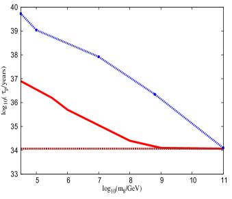
Figure 3: Variation of proton lifetime as a function of color octet mass $M_{C}$ for Model-I (upper curve) and Model-II (lower curve). The horizontal line is the present experimental limit.

3 TYPE-II SEESAW DOMINANCE

In this section we discuss prospects of having a type-II seesaw dominated neutrino mass formula in the two $SO(10)$ based models discussed in Sec.2.

3.1 Derivation of type-II seesaw formula

We have added to the usual spinorial representations ${16}_{F_{i}}(i=1,2,3)$ for fermion representations in $SO(10)$, one fermion singlet per generation $S_{i}(i=1,2,3)$. The $G_{2213}$ symmetric Yukawa Lagrangian descending from $SO(10)$ symmetry can be written as

$$\mathcal{L}_{\rm Yuk} = \sum_{i=1,2}Y_{i}^{\ell}\left(\overline{\psi}_{L}\,\psi_{R}\,\Phi_{i}\right)+f(\,\psi^{c}_{R}\,\psi_{R}\Delta_{R}+\psi^{c}_{L}\,\psi_{L}\Delta_{L})$$ (10)

$$+ y_{\chi}\,\left(\overline{\psi}_{R}\,S\,\chi_{R}+\overline{\psi}_{L}\,S\,\chi_{L}\right)+\left(\text{h.c.}\right),$$

where $\Phi_{1,2}\subset{10_{{H_{1}},{H_{2}}}}$ are two bidoublets, $(\Delta_{L},\Delta_{R})\subset{126}_{F}$ and $(\chi_{L},\chi_{R})\subset{16}_{H}$. As discussed in Sec.2, the spontaneous breaking of $G_{2213}\longrightarrow G_{2113}$, takes place by the VEV of the RH triplet $\sigma_{R}(1,3,0,1)\subset 45_{H}$ carrying $B-L=0$ which doesnot generate any fermion mass term. As we discuss below, when the Higgs scalar $\Phi_{i}$, $\Delta_{R}$ and $\chi_{R}$ acquire VEV’s spontaneous symmetry breakings leading to $G_{2113}\longrightarrow SM\longrightarrow U(1)_{em}\times SU(3)_{C}$ occur and generate $N-S$ mixing mass term $M=y_{\chi}\langle{\chi_{R}^{0}}\rangle$ by the induced VEVs.In addition $v_{\chi_{L}}=\langle{\chi_{L}^{0}}\rangle$ and $v_{L}=\langle{\Delta_{L}^{0}}\rangle$ are automatically generated even though the LH doublet $\chi_{L}$ and the RH triplet $\Delta_{L}$ are assigned vanishing VEVs directly. In models with inverse seesaw [36] or extended seesaw [17, 18, 37, 38] mechanisms, a bare mass term of the singlet fermions $\mu_{S}S^{T}S$ occurs in the Lagrangian. Being unrestricted as a gauge singlet mass term in the Lagrangian, determination of its value has been left to phenomenological analyses in neutrino physics. Larger values of the parameter near the GUT-Planck scale [39] or at the intermediate scale [40] have been also exploited. On the other hand, fits to the neutrino oscillation data through inverse seesaw formula by a number of authors have shown to require much smaller values of $\mu_{S}$ [18, 37, 14, 17, 43]. Even phenomenological implications of its vanishing value have been investigated recently in the presence of other non-standard and non-vanishing fermion masses [41, 42] in the $9\times 9$ mass matrix. Very small values of $\mu_{S}$ is justified on the basis of ’t Hooft’s naturalness criteria representing a mild breaking of global lepton number symmetry of the SM [44]. While we consider the implication of this term later in this section, at first we discuss the emerging neutrino mass matrix by neglecting it. In addition to the VEVs discussed in Sec.2 for gauge symmetry breaking at different stages, we assign the VEV to the neutral component of RH Higgs doublet of ${16}_{H}$ with $<\chi_{R}(1,1/2,-1/2,1)>=V_{\chi}$ in order to generate $N-S$ mixing mass term ${\rm M}{\overline{N}}S$ between the RH neutrino and the sterile fermion where the $3\times 3$ matrix ${\rm M}=y_{\chi}V_{\chi}$. We define the other $3\times 3$ mass matrices $M_{D}=Y^{(1)}v_{u}$ and $M_{N}=fV_{R}$. We also include induced small contributions to the vacuum expectation values of the LH Higgs triplet $v_{L}=<\Delta_{L}(3,0,-2,1)>$ and the LH Higgs doublet $v_{\chi_{L}}=<\chi_{L}(2,0,-2,1)>$ leading to the possibilities $\nu-S$ mixing with $M_{L}=y_{\chi}v_{\chi_{L}}$ and the induced type-II seesaw contribution to LH neutrino masses $m_{\nu}^{II}=fv_{L}$ given in eq.(20). The induced VEVs are shown in the left and right panels of Fig.4. We have also derived them by actual potential minimisation which agree with the diagramatic contribution. Including the induced VEV contributions, the mass term due to Yukawa Lagrangian can be written as

$$\mathcal{L}_{mass} = (M_{D}\overline{\nu}N+\frac{1}{2}M_{N}N^{T}N+M\overline{N}S$$ (11)

$$+\left.M_{L}\overline{\nu}S+h.c\right)+m_{\nu}^{II}{\nu^{T}}\nu$$

In the $(\nu,S,N^{C})$ basis the generalised form of the $9\times 9$ neutral fermion mass matrix after electroweak symmetry breaking can be written as

$${\cal M}=\begin{pmatrix}m_{\nu}^{II}&M_{L}&M_{D}\\ M_{L}^{T}&0&M^{T}\\ M_{D}^{T}&M&M_{N}\end{pmatrix}.$$ (12)

where $M_{D}=Y\langle\Phi\rangle$, $M_{N}=fv_{R}$, ${\rm M}=y_{\chi}\langle\chi_{R}^{0}\rangle$,$M_{L}=y_{\chi}\langle\chi_{L}^{0}\rangle$ and we have used $\mu_{s}=0$. In this model the symmetry breaking mechanism and the VEVs are such that $M_{N}>M\gg M_{D}$. The RH neutrino mass being the heaviest fermion mass scale in the Lagrangian, this fermion is at first integrated out leading to the effective Lagrangian at lower scales [45, 32, 46],

$$-\mathcal{L}_{\rm eff}=\left(m_{\nu}^{II}+M_{D}\frac{1}{M_{N}}M^{T}_{D}\right)_{\alpha\beta}\,\nu^{T}_{\alpha}\nu_{\beta}+$$

$$\left(M_{L}+M_{D}\frac{1}{M_{N}}M^{T}\right)_{\alpha m}\,\left(\overline{\nu_{\alpha}}S_{m}+\overline{S_{m}}\nu_{\alpha}\right)$$

$$+\left(M\frac{1}{M_{N}}M^{T}\right)_{mn}\,S^{T}_{m}S_{n},$$ (13)

Whereas the heaviest RH neutrino mass matrix $M_{N}$ separates out trivially, the other two $3\times 3$ mass matrices $\mathcal{M}_{\nu}$, and $m_{S}$ are extracted through various steps of block diagonalisation [18].The details of various steps are given in Appendix B and the results are

$$\mathcal{M_{\nu}}=m_{\nu}^{II}+\left(M_{D}M_{N}^{-1}M^{T}_{D}\right)-(M_{D}M_{N}^{-1}M^{T}_{D})$$

$$+M_{L}(M^{T}M_{N}^{-1}M)^{-1}M_{L}^{T}$$

$$-M_{L}(M^{T}M_{N}^{-1}M)^{-1}(M^{T}M_{N}^{-1}M_{D}^{T})$$

$$-(M_{D}M_{N}^{-1}M)(M^{T}M_{N}^{-1}M)^{-1}M_{L}^{T},$$

$$m_{s}=-MM_{N}^{-1}M^{T}+....,$$

$$m_{N}=M_{N}.$$ (14)

From the first of the above three equations, it is clear that the type-I seesaw term cancels out [45, 32, 46] with another of opposite sign resulting from block diagonalisation. Then the generalised form of the light neutrino mass matrix turns out to be

$${\cal M}_{\nu} = ~{}fv_{L}+M_{L}M^{-1}M_{N}(M^{T})^{-1}M_{L}^{T}$$ (15)

$$-[M_{L}M_{D}^{T}M^{-1}+M_{L}^{T}M_{D}(M^{T})^{-1}].$$

With $M_{L}=y_{\chi}v_{\chi_{L}}$ that induces $\nu-S$ mixing, the second term in this equation is double seesaw formula and the third term is the linear seesaw formula which are similar to those derived earlier [40].

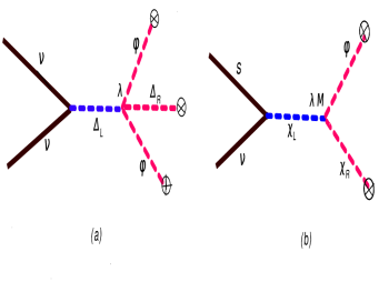
Figure 4: Feynman diagrams for induced contributions to VEVs of the LH triplet (diagram (a)) and the LH doublet (diagram (b)) in Model-I and Model-II.

From the Feynman diagrams, the analytic expressions for the induced VEVs are

$$v_{L} \sim \frac{V_{R}}{M_{\Delta_{L}}^{2}}\left(\lambda_{1}v_{1}^{2}+\lambda_{2}v_{2}^{2}\right),$$

$$v_{\chi_{L}} \sim \frac{V_{\chi}}{M_{\chi_{L}}^{2}}\left(\lambda^{\prime}_{1}M^{\prime}_{1}v_{1}+\lambda^{\prime}_{2}M^{\prime}_{2}v_{2}\right),$$ (17)

$$= C_{\chi}\frac{V_{\chi}M_{R^{+}}v_{wk}}{M_{\chi_{L}}^{2}},$$

where $v_{wk}\sim 100$ GeV, and

$$C_{\chi} = {\left(\lambda^{\prime}_{1}M^{\prime}_{1}v_{1}+\lambda^{\prime}_{2}M^{\prime}_{2}v_{2}\right)\over(M_{R^{+}}v_{wk})}.$$ (18)

In eq.(17), $v_{i}(i=1,2)$ are the VEVs of two electroweak doublets each originating from separate ${10}_{H}\subset SO(10)$ as explained in the following section, and $M^{\prime}_{1},M^{\prime}_{2}$ are Higgs trilinear coupling masses which are normally expected to be of order $M_{R^{+}}$. In both the models $V_{R}=5-10$ TeV and $V_{\chi}\sim 300-1000$ GeV. Similar expressions as in eq.(17) are also obtained by minimisation of the scalar potential.

3.2 Suppression of linear seesaw and dominance of type-II seesaw

Now we discuss how linear seesaw term is suppressed without fine tuning of certain parameters in Model-I but with fine tunning of the same parameters in Model-II. The expression for neutrino mass is given in eq.(15) where the first, second, and the third terms are type-II seesaw, double seesaw, and linear seesaw formulas for the light neutrino masses. Out of these, for all parameters allowed in both the models (Model-I and Model-II), the double seesaw term will be found to be far more suppressed compared to the other two terms. Therefore we now discuss how the linear seesaw term is suppressed compared to the type-II seesaw term allowing the dominance of the latter. In Model-I, gauge coupling unification has been achieved such that $M_{P}=M_{\chi_{L}}\sim M_{U}\geq 10^{15.6}$ GeV, $M_{\Delta_{L}}=10^{8}$ GeV where $M^{\prime}_{1}\sim M^{\prime}_{2}\sim M_{R^{+}}\sim 10^{9}$ GeV. Using these masses in eq.(15), we find that even with $C_{\chi}\sim 0.1-1.0$

$$v_{\chi_{L}} \sim 10^{-18}~{}{\rm eV}-10^{-17}~{}{\rm eV},$$

$$v_{L} \simeq 0.1~{}{\rm eV}-0.5~{}{\rm eV},$$

Such induced VEVs in the Model-I suppress the second and the third terms in eq.(15) making the model quite suitable for type-II seesaw dominance although the Model-II needs fine tuning in the induced contributions to the level of $C_{\chi}\leq 10^{-5}$ as discussed below.
In Model-II, $M_{\Delta_{L}}\sim M_{\chi_{L}}\sim M_{P}\sim 10^{9}$ GeV , and without any fine tuning of the parameters in eq.(LABEL:vl), we obtain $v_{L}\sim 10^{-10}$  GeV. From eq.(17) we get $v_{\chi_{L}}\sim C_{\chi}\times 10^{-6}~{}{\rm{GeV}}\sim 10^{-7}{\rm{GeV}}$ for $C_{\chi}\sim 0.1$. With ${(M_{D})}_{(3,3)}\leq 100$ GeV and ${M_{D}\over M}\simeq 0.1-1$, the most dominant third term in eq.(15) gives $M_{\nu}\geq 10^{-8}~{}{\rm GeV}$. This shows that fine tuning is needed in the parameters occuring to reduce $C_{\chi}\leq 10^{-5}$ to suppress linear seesaw and permit type-II seesaw dominance in Model-II whereas the type-II seesaw dominance is achieved in Model-I with $C_{\chi}\simeq 0.1-1.0$ without requiring any such fine tuning. In what follows we will utilise the type-II seesaw dominated neutrino mass formula to study neutrino physics, neutrino-less double beta decay, and lepton flavor violations in the context of Model-I although they are similar in Model-II subject to the fine tuning constraint on $C_{\chi}$. Thus the light neutrino mass is dominated by the type-II seesaw term

$${\mathcal{M}}_{\nu} \simeq ~{}fv_{L}.$$ (20)

3.3 Right-handed neutrino mass prediction

Global fits to the experimental data [47] on neutrino oscillations have determined the mass squared differences and mixing angles at $3\sigma$ level

$$\sin^{2}\theta_{12}=0.320,\,\,\,\,\sin^{2}\theta_{23}=0.427,$$

$$\sin^{2}\theta_{13}=0.0246,\,\,\delta_{CP}=0.8\pi,$$

$$\Delta m_{\rm sol}^{2}=7.58\times 10^{-5}{\rm eV}^{2},$$

$$|\Delta m_{\rm atm}|^{2}=2.35\times 10^{-3}{\rm eV}^{2}.$$ (21)

For normally hierarchical (NH), inverted hierarchical (IH), and quasi-degenerate (QD) patterns, the experimental values of mass squared differences can be fitted by the following values of light neutrino masses

$${\hat{m}}_{\nu} = (0.00127,0.008838,0.04978)~{}{\rm eV}\,\,(\rm{NH})$$ (22)

$$= (0.04901,0.04978,0.00127)~{}{\rm eV}\,\,(\rm{IH})$$

$$= (0.2056,0.2058,0.2)~{}{\rm eV}\,\,(\rm{QD})$$

We use the diagonalising Pontecorvo-Maki-Nakagawa-Sakata (PMNS) matrix. The $U_{PMNS}$ matrix is give by

$$\begin{pmatrix}c_{13}c_{12}&c_{13}s_{12}&s_{13}e^{-i\delta}\\ -c_{23}s_{12}-c_{12}s_{13}s_{23}e^{i\delta}&c_{12}c_{23}-s_{12}s_{13}s_{23}e^{i\delta}&s_{23}c_{13}\\ s_{12}s_{23}-c_{12}c_{23}s_{13}e^{i\delta}&-c_{12}s_{23}-s_{12}s_{13}c_{23}e^{i\delta}&c_{13}c_{23}\\ \end{pmatrix},$$ (23)

and determine it using mixing angle and the leptonic Dirac phase from eq. (21)

$$U_{\rm{PMNS}}=\begin{pmatrix}0.814&0.55&-0.12-0.09i\\ -0.35-0.049i&0.67-0.034i&0.645\\ 0.448-0.057i&-0.48-0.039i&0.74\end{pmatrix}.$$ (24)

Now inverting the relation ${\hat{m}}_{\nu}=U_{PMNS}^{\dagger}{\mathcal{M}}_{\nu}U_{PMNS}^{*}$ where ${\hat{m}}_{\nu}$ is the diagonalised neutrino mass matrix, we determine ${\mathcal{M}}_{\nu}$ for three different cases and further determine the corresponding values of the $f$ matrix using $f={\mathcal{M}}_{\nu}/v_{L}$ where we use the predicted value of $v_{L}=0.1$ eV. Noting that
$M_{N}=fV_{R}={{\mathcal{M}}_{\nu}V_{R}}/v_{L}$, we have also derived eigen values of the RH neutrino mass matrix ${\hat{M}}_{N_{i}}$ as the positive square root of the $i^{th}$ eigen value of the Hermitian matrix $M_{N}^{{\dagger}}M_{N}$.
NH

$$f=\begin{pmatrix}0.117+0.022i&-0.124-0.003i&0.144+0.025i\\ -0.124-0.003i&0.158-0.014i&-0.141+0.017i\\ 0.144+0.025i&-0.141+0.017i&0.313-0.00029i\end{pmatrix}$$ (25)

$$|{\hat{M}}_{N}|={\rm diag}(160,894,4870)~{}{\rm GeV}.\,\$$ (26)

IH

$$f=\begin{pmatrix}0.390-0.017i&0.099+0.01i&-0.16+0.05i\\ 0.099+0.01i&0.379+0.02i&0.176+0.036i\\ -0.16+0.05i&0.176+0.036i&0.21-0.011i\end{pmatrix}$$ (27)

$$|{\hat{M}}_{N}|={\rm diag}(4880,4910,131)~{}{\rm GeV}.\,\$$ (28)

QD

$$f=\begin{pmatrix}2.02+0.02i&0.0011+0.02i&-0.019+0.3i\\ 0.0011+0.02i&2.034+0.017i&0.021+0.21i\\ -0.019+0.3i&0.021+0.21i&1.99-0.04i\end{pmatrix}$$ (29)

For $v_{L}=0.1$ eV, we have

$$|{\hat{M}}_{N}|={\rm diag}(21.46,20.34,18.87)~{}{\rm TeV}\$$ (30)

but for $v_{L}=0.5$ eV, we obtain

$$|{\hat{M}}_{N}|={\rm diag}(4.3,4.08,3.77)~{}{\rm TeV}.\$$ (31)

These RH neutrino masses predicted with $v_{L}=0.1$ eV for NH and IH cases and with $v_{L}=0.5$ eV for the QD case are clearly verifiable by the LHC.

4 THE DIRAC NEUTRINO MASS MATRIX

The Dirac neutrino mass matrix which has its quark-lepton symmetric origin [8] plays a crucial role in the predictions of lepton flavor violations (LFVs) [14, 17] as well as lepton number violations (LNVs) as pointed out very recently [18, 37]. The determination of the Dirac neutrino mass matrix $M_{D}(M_{R^{0}})$ at the TeV seesaw scale is done which was discussed in [17, 48].

4.1 Extrapolation to the GUT scale

The RG extrapolated values at the GUT scale are,
$\mu={\rm M_{GUT}}$:

$$m^{0}_{e} = 0.00048~{}{\rm GeV},m^{0}_{\mu}={\rm 0.0875}~{}{\rm GeV},m^{0}_{\tau}=1.8739~{}{\rm GeV},$$

$$m^{0}_{d} = 0.0027~{}{\rm GeV},m^{0}_{s}=0.0325~{}{\rm GeV},m^{0}_{b}=1.3373~{}{\rm GeV},$$

$$m^{0}_{u} = 0.001~{}{\rm GeV},m^{0}_{c}=0.229~{}{\rm GeV},m^{0}_{t}=78.74~{}{\rm GeV},$$ (32)

The $V^{0}_{\rm CKM}$ matrix at the GUT scale is given by

$$V^{0}_{\rm CKM}=\footnotesize\begin{pmatrix}0.97&0.22&-0.0003-0.003i\\ -0.22-0.0001i&0.97&0.036\\ 0.008-0.003i&-0.035+0.0008i&0.99\end{pmatrix}.$$ (33)

For fitting the charged fermion masses at the GUT scale, in addition to the two complex ${10}_{H_{1,2}}$ representations with their respective Yukawa couplings $Y_{1,2}$, we also use the higher dimensional operator [14, 17]

$${\bf\frac{\kappa_{ij}}{M_{G}^{2}}16_{i}16_{j}{10}_{H}{45}_{H}{45}_{H}},$$ (34)

In the above equation the product of three Higgs scalars acts as an effective ${126}_{H}^{\dagger}$ operator [14]. With $M_{G}\simeq M_{Pl}$ or $M\simeq M_{string}$, this is suppressed by $(M_{U}/M_{G})^{2}\simeq 10^{-3}-10^{-5}$ for GUT-scale VEV of ${45}_{H}$. Then the formulas for different charged fermion mass matrices are

$$M_{u} = {G}_{u}+{F},~{}~{}M_{d}={G}_{d}+{F},$$

$$M_{e} = {G}_{d}-3{F},~{}~{}M_{D}={G}_{u}-3{F}.$$ (35)

Following the procedure given in [17], the Dirac neutrino mass matrix at the GUT scale is found to be

$$M_{D}(M_{R^{0}})=\footnotesize\begin{pmatrix}0.014&0.04-0.01i&0.109-0.3i\\ 0.04+0.01i&0.35&2.6+0.0007i\\ 0.1+0.3i&2.6-0.0007i&79.20\end{pmatrix}{GeV}.$$ (36)

5 LEPTON FLAVOR VIOLATION

In the present non-SUSY SO(10) models, even though neutrino masses are governed by high scale type-II seesaw formula, the essential presence of singlet fermions that implement the type-II seesaw dominance by cancelling out the type-I seesaw contribution give rise to experimentally observable LFV decay branching ratios through their loop mediation. The heavier RH neutrinos in this model being in the range of $\sim 1-10$ TeV mass range also contribute, but less significantly than the singlet fermions. The charged current weak interaction Lagrangian in this model can be written in the generalised form,

5.1 Estimation of non-unitarity matrix

Using flavor basis, the general form of charged current weak interaction Lagrangian including both $V\pm A$ currents in the Model-I and Model-II is

$$\mathcal{L}_{\rm CC} = -\frac{1}{\sqrt{2}}\,\sum_{\alpha=e,\mu,\tau}\bigg{[}g_{2L}\overline{\ell}_{\alpha\,L}\,\gamma_{\mu}{\nu}_{\alpha\,L}\,W^{\mu}_{L}+g_{2R}\overline{\ell}_{\alpha\,R}\,\gamma_{\mu}{N}_{\alpha\,R}\,W^{\mu}_{R}\bigg{]}$$ (37)

$$+\text{h.c.}$$

In both the models, the $W^{\pm}_{R}$ bosons and the doubly charged Higgs scalars, both left-handed (LH) and right handed (RH), are quite heavy with $M_{W_{R}}\sim M_{\Delta}\simeq 10^{8}-10^{9}$ GeV. These make negligible contributions arising out of the RH current effects and Higgs exchange effects on LFV or LNV decay amplitudes. In the two models considered here, the flavor eigenstate of any LH neutrino $\nu$ can be represented in terms of mass eigen states $\nu_{i}$, $S_{i}$, and $N_{i}$. From details of model parametrisation discussed in Sec.3-Sec.5, we have found the corresponding mixing matrices with active neutrinos, ${\cal V}^{\nu N}=M_{D}/M_{N}\equiv X_{N}$, and ${\cal V}^{\nu S}=M_{D}/M\equiv X_{S}$

$$\nu = {\cal N}\nu_{i}+{\cal V}^{\nu N}N_{i}+{\cal V}^{\nu S}S_{i},$$

$${\cal N} \simeq [1-(\eta^{N}+\eta^{S})]U_{\rm{\small PMNS}},$$

$$\eta^{N} = (X_{N}.X_{N}^{\dagger})/2,$$

$$\eta^{S} = (X_{S}.X_{S}^{\dagger})/2.$$ (38)

These mixings modify the standard weak interaction Lagrangian in the LH sector by small amounts but they could be in the experimentally accessible range [56]. In the LH sector the charged current weak interaction Lagrangian is

$${\cal L}_{\rm CC} = -\frac{g_{2L}}{\sqrt{2}}W_{\mu}{\bar{e}}\gamma^{\mu}P_{L}\left({\cal N}\nu_{i}+{\cal V}^{\nu N}N_{i}+{\cal V}^{\nu S}S_{i}\right)$$ (39)

$$+h.c.$$

The implications of these terms for LFV and LNV effects have been discussed below. From eq.(38) it is clear that ${\cal N}$ is non-unitary. We assume the $N-S$ mixing matrix ${\rm M}$ to be diagonal for the sake of simplicity and economy of parameters,

$$M={\rm diag}~{}(M_{1},M_{2},M_{3}),$$ (40)

Noting that the non-unitarity deviation is characterised by $\eta=\eta^{S}+\eta^{N}$ which in the limit $M_{N}>>M$ turn out to be

$$\eta \simeq \eta^{S}=\frac{1}{2}X_{S}.X_{S}^{{\dagger}}=M_{D}M^{-2}M_{D}^{{\dagger}},$$

$$\eta_{\alpha\beta} = \frac{1}{2}\sum_{k=1,2,3}\frac{M_{D_{\alpha k}}M_{D_{\beta k}}^{*}}{M_{k}^{2}}.$$ (41)

For the degenerate case, $M_{i}=M_{Deg}(i=1,2,3)$, gives,

$$\eta=\frac{1{\rm GeV}^{2}}{M_{Deg}^{2}}\times$$

$$\footnotesize{\begin{pmatrix}0.0394&0.146-0.403i&4.17-11.99i\\ 0.146+0.403i&3.602&105.8-0.002i\\ 4.173+11.9i&105.805+0.002i&3139.8\end{pmatrix}.}$$ (42)

For the general non-degenerate case of ${\rm M}$, we saturate the upper bound $|\eta_{\tau\tau}|<2.7\times 10^{-3}$ [50] to derive

$$\frac{1}{2}\left[\frac{0.1026}{M_{1}^{2}}+\frac{7.0756}{M_{2}^{2}}+\frac{6762.4}{M_{3}^{2}}\right]=2.7\times 10^{-3},$$ (43)

By inspection, this equation gives the lower bounds

$$M_{1} > 4.35~{}{\rm GeV},~{}M_{2}>36.2~{}{\rm GeV},M_{3}>1120~{}{\rm GeV},$$ (44)

and for the degenerate case $M_{Deg}=1213$ GeV. For the partially degenerate case of $M_{1}=M_{2}\neq M_{3}$, the solutions can be similarly derived as in ref[17] and one example is $M(100,100,1319.67)$ GeV .

5.2 Branching ratio and CP Violation

One of the most important outcome of non-unitarity effects is expected to manifest through ongoing experimental searches for LFV decays such as $\tau\to e\gamma$, $\tau\to\mu\gamma$, $\mu\to e\gamma$. In these models the RH neutrinos and the singlet fermions contribute to the branching ratios [14, 17, 15]. Because of the condition $M_{N}>>M$, neglecting the RH neutrino exchange contribution compared to the sterile fermion singlet contributions, our estimations for different cases of $M$ values are presented below. These values are many orders larger than the standard non-SUSY contributions and are accessible to ongoing or planned searches [4]. For the degenerate case

$$\Delta{{\cal J}}^{12}_{e\mu} = -2.1\times 10^{-6},$$

$$\Delta{{\cal J}}^{23}_{e\mu} = -2.4\times 10^{-6},$$

$$\Delta{{\cal J}}^{23}_{\mu\tau} = 1.4\times 10^{-4},$$

$$\Delta{{\cal J}}^{31}_{\mu\tau} = 1.2\times 10^{-4},$$

we have the predicted values of the branching ratios

$$BR(\mu\to e\gamma) = 6.43\times 10^{-17},$$

$$BR(\tau\to e\gamma) = 8.0\times 10^{-16},$$

$$BR(\tau\to\mu\gamma) = 2.41\times 10^{-12}.$$ (46)

Because of the presence of non-unitarity effects in the present model , the leptonic CP-violation turn out to be similar as in refs.[17, 50, 51]. The moduli and phase of non-unitarity and CP-violating parameter for the degenerate case of the present models are

$$|\eta_{e\mu}| = 2.73\times 10^{-8},$$

$$\delta_{e\mu} = 1.920,$$

$$|\eta_{e\tau}| = 4.54\times 10^{-7},$$

$$\delta_{e\tau} = 1.78,$$

$$|\eta_{\mu\tau}| = 2.31\times 10^{-5},$$

$$\delta_{\mu\tau} = 2.39\times 10^{-7}.$$ (47)

The estimations presented in eq.(47) show that in a wider range of the parameter space, the leptonic CP violation parameter could be nearly two orders larger than the CKM-CP violation parameter for quarks.

6 NEUTRINO-LESS DOUBLE BETA DECAY

Even with the vanishing bare mass term $\mu_{S}=0$ in the Yukawa Lagrangian of eq.(10), the singlet fermions $S_{i}(i=1,2,3)$ acquire Majorana masses over a wide range of values and, in the leading order, the corresponding mass matrix given in eq.(14) is $m_{S}=-M\frac{1}{M_{N}}M^{T}$. As far as light neutrino mass matrix is concerned, it is given by the type-II seesaw formula of eq.(20) which is independent of the Majorana mass matrix $m_{S}$ of singlet fermions. But the combined effect of substantial mixing between the light neutrinos and the singlet or the RH neutrinos, and also between the singlet neutrinos and the RH neutrinos result in the new Majorana neutrino mass insertion terms in the Feynman diagrams. Out of these the mass insertion $m_{S}$ due to the singlet fermions in the Feynman diagram gives rise to new dominant contributions to the amplitude and the effective mass parameter for $0\nu\beta\beta$ even in the $W_{L}-W_{L}$ channel. This may be contrasted with the conventional type-II seesaw dominated non-SUSY $SO(10)$ models with only three generations of standard fermions in ${\bf{16}_{i}}(i=1,2,3)$ where there is no such contributions to $0\nu\beta\beta$ decay. The generalised form of charged current interaction Lagrangian for leptons in this model including both $V\pm A$ currents has been given in eq.(37).

As stated above, in the Model-I and Model-II, the $W^{\pm}_{R}$ bosons and the doubly charged Higgs scalars, both left-handed and the right handed, are quite heavy with $M_{W_{R}}\sim M_{\Delta}\simeq 10^{8}-10^{9}$ GeV. These make negligible contributions due to the RH current effects and Higgs exchange effects for the $0\nu\beta\beta$ decay amplitude. The most popular standard and conventional contribution in the $W^{-}_{L}-W^{-}_{L}$ channel is due to light neutrino exchanges. But one major new point in this work is that even in the $W^{-}_{L}-W^{-}_{L}$ channel, the singlet fermion exchange allowed within the type-II seesaw dominance mechanism, can yield much more dominant contribution to $0\nu\beta\beta$ decay rate. For the exchange of singlet fermions ($\hat{S}_{j}$), the Feynman diagram is shown in the Fig.5. For the exchange of heavier RH Majorana neutrinos ($\hat{N}_{k}$), the diagram is the same as the right-panel of this figure but with the replacement of the mixing matrix and masses by ${\mathcal{V}}^{\nu S}\to{\mathcal{V}}^{\nu N}$ and $m_{S_{i}}\to M_{N_{i}}$. The heavier RH neutrino exchange contributions are found to be negligible compared to the singlet fermion exchange contributions. In the mass basis, the contributions to the decay amplitudes by $\nu$ and $S$ exchanges are estimated as

$$\mathcal{A}^{LL}_{\nu}\propto\frac{1}{M^{4}_{W_{L}}}\sum_{i=1,2,3}\frac{\left(\mathcal{V}^{\nu\nu}_{e\,i}\right)^{2}\,m_{\nu_{i}}}{p^{2}}$$ (48)

$$\mathcal{A}^{LL}_{S}\propto\frac{1}{M^{4}_{W_{L}}}\sum_{j=1,2,3}\frac{\left(\mathcal{V}^{\nu S}_{e\,j}\right)^{2}}{m_{S_{j}}}$$ (49)

$$\mathcal{A}^{LL}_{N}\propto\frac{1}{M^{4}_{W_{L}}}\sum_{j=1,2,3}\frac{\left(\mathcal{V}^{\nu N}_{e\,j}\right)^{2}}{m_{N_{j}}},$$ (50)

where $|p|\simeq 190~{}\mbox{MeV}$ represents the magnitude of neutrino virtuality momentum [52, 54]. Using uncertainities in the nuclear matrix elements [53, 54] we have found it to have values in the range $|p|=120{\rm MeV}-200{\rm MeV}$. In order to understand physically how the singlet fermion Majorana mass insertion terms as a new source of lepton number violation contributes to $0\nu\beta\beta$ process, we draw the Feynman diagram Fig.5. with mass insertion.

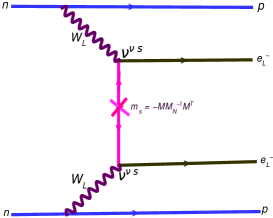
Figure 5: Feynman diagrams for neutrinoless double beta decay contribution with virtual Majorana neutrinos $\hat{\nu}_{i}$, and $\hat{S}_{i}$ in the $W_{L}-W_{L}$-channel. For the RH neutrino exchange the Feynman diagram is same as in the right-panel but with the replacements ${\mathcal{V}}^{\nu S}\to{\mathcal{V}}^{\nu N}$, $S_{i}\to N_{i}$

In this model, the Majorana mass matrix for the singlet fermion after block diagonalisation is $m_{S}=-MM_{N}^{-1}M^{T}$. Then exchanges of such singlets generate dominant contribution through their mixings to active neutrinos and this mixing is proportional to the Dirac neutrino mass $M_{D}$ derived in 4. It is clear from Fig. 5 that the the singlet fermion exchange amplitudes assume the same form as in eq.(49).

7 EFFECTIVE MASS PARAMETER AND HALF LIFE

Adding together the $0\nu\beta\beta$ decay amplitudes arising out of light neutrino exchanges, singlet fermion exchanges, and the heavy RH neutrino exchanges in the $W_{L}-W_{L}$ channel from eq.(49), and using suitable normalisations [53, 54], we express the inverse half life

$$\left[T_{1/2}^{0\nu}\right]^{-1} \simeq G^{0\nu}_{01}|\frac{{\cal M}^{0\nu}_{\nu}}{m_{e}}|^{2}|({\large\bf m}^{ee}_{\nu}+{\large\bf m}^{ee}_{S}+{\large\bf m}^{ee}_{N})|^{2},$$ (51)

$$= K_{0\nu}|({\large\bf m}^{ee}_{\nu}+{\large\bf m}^{ee}_{S}+{\large\bf m}^{ee}_{N})|^{2},$$

$$= K_{0\nu}|{\large\bf m}_{\rm eff}|^{2}$$

In the above equation $G^{0\nu}_{01}=0.686\times 10^{-14}{\rm yrs}^{-1}$, ${\cal M}^{0\nu}_{\nu}=2.58-6.64$, $K_{0\nu}=1.57\times 10^{-25}{\rm yrs}^{-1}{\rm eV}^{-2}$, and the three effective mass parameters for light neutrino, singlet fermion, and heavy RH neutrino exchanges are

$${\large\bf m}^{\rm ee}_{\nu}=\sum_{i}\left(\mathcal{V}^{\nu\nu}_{e\,i}\right)^{2}\,{m_{\nu_{i}}}$$ (52)

$${\large\bf m}^{\rm ee}_{S}=\sum_{i}\left(\mathcal{V}^{\nu S}_{e\,i}\right)^{2}\,\frac{|p|^{2}}{m_{S_{i}}}$$ (53)

$${\large\bf m}^{\rm ee}_{N}=\sum_{i}\left(\mathcal{V}^{\nu N}_{e\,i}\right)^{2}\,\frac{|p|^{2}}{m_{N_{i}}},$$ (54)

with

$${\large\bf m}_{\rm eff}={\large\bf m}^{ee}_{\nu}+{\large\bf m}^{ee}_{S}+{\large\bf m}^{ee}_{N}.$$ (55)

Here $m_{S_{i}}$ is the eigen value of the $S-$ fermion mass matrix $m_{S}$, and the magnitude of neutrino virtuality momentum $|p|=120$ MeV$-200$ MeV. As the predicted values of the RH neutrino masses carried out in Sec.3 have been found to be large which make their contribution to the $0\nu\beta\beta$ decay amplitude negligible, we retain only contributions due to light neutrino and singlet fermion exchanges. The estimated values of the effective mass parameters due to the $S-$ fermion exchanges and light neutrino exchanges are shown separately in Fig. 6 where the magnitudes of corresponding mass eigen values used have been also indicated.

7.1 Numerical estimations of effective mass parameters

Using the equations of normalized mass parameters [18] , we estimate numerically the nearly standard contribution due to light neutrino exchanges and the dominant non-standard contributions due to singlet fermion exchanges.

A.Nearly standard contribution
In this model the new mixing matrix $\mathcal{N}\equiv\mathcal{V}^{\nu\nu}=\left(1-\eta\right)U_{\nu}$ contains additional non-unitarity effect due to non-vanishing $\eta$ [18] Using $M_{Deg}=1213$ GeV in the degenerate case, we estimate

$${\mathcal{N}}_{ei}=~{}(0.81437,~{}0.54858,~{}0.1267+0.0922i).$$ (56)

Since all the $\eta-$ parameters are constrained by $|\eta_{\alpha\beta}|<10^{-3}$, it is expected that $|{\mathcal{N}}_{ei}|\simeq|U_{ei}|$ for any other choice of $M$. In the leading approximation, by neglecting the $\eta_{\alpha i}$ contributions , the effective mass parameter in the the $W_{L}-W_{L}$ channel with light neutrino exchanges is expressed as

$$m^{\rm ee}_{\nu} = \sum_{i}{\mathcal{N}}_{ei}^{2}{\hat{m}}_{i}$$ (57)

$$\simeq(c_{12}c_{13})^{2}{\hat{m}}_{1}e^{i\alpha_{1}}+(s_{12}c_{13})^{2}{\hat{m}}_{2}e^{i\alpha_{2}}$$

$$+s_{13}^{2}e^{i\delta}{\hat{m}}_{3},$$

where we have introduced two Majorana phases $\alpha_{1}$ and $\alpha_{2}$. As discussed subsequently in this section, they play crucial roles in preventing cancellation between two different effective mass parameters. Using $\alpha_{1}=\alpha_{2}=0$ and the experimental values of light neutrino masses and the Dirac phase $\delta=0.8\pi$ from eq.(21), the light neutrino exchanges have their well known values,

$$|m^{\rm ee}_{\nu}| =\left\{\begin{array}[]{cc}0.0039\,\mbox{eV}&\mbox{ NH,}\\[5.69046pt] 0.04805\,\mbox{eV}&\mbox{ IH,}\\[5.69046pt] 0.23\,\mbox{eV}&\mbox{ QD.}\end{array}\right.$$ (61)

B. Dominant non-standard contributions
The $(ei)$ element of the $\nu-S$ mixing matrix is [18]

$${\mathcal{V}}^{\nu S}_{ei}=(\frac{M_{D}}{M})_{ei}.$$ (62)

where the Dirac neutrino mass matrix $M_{D}$ has been given in eq.(36), and the diagonal elements are estimated using the non-unitarity equation as discussed in the previous section. We derive the relevant elements of the mixing matrix $\mathcal{V}^{\nu S}$ using the structures of the the Dirac neutrino mass matrix $M_{D}$ given in eq.(36) and values of the diagonal elements of $M=(M_{1},M_{2},M_{3})$ satisfying the non-unitarity constraint in eq.(43). The eigen values of the $S-$ fermion mass matrix $m_{S}$ are estimated for different cases using the structures of the RH Majorana neutrino mass matrices given in eq.(26), eq.(28), and eq.(30) in the formula $m_{S}=-M\frac{1}{M_{N}}M^{T}$. It is clear that in the effective mass parameter the non-standard contribution due to sterile fermion exchange has a sign opposite to that due to light neutrino exchange and also its magnitude is inversely proportional to the sterile fermion mass eigen values. In the NH case the estimated effective mass parameters are shown in Fig.6 where the values of diagonal elements of $M$ and the eigen values of $m_{s}$ have been specified. For comparison the effective mass parameters in the standard case without singlet fermions have been also given. It is clear that for allowed masses of the model, the non-standard contributions to effective mass parameters can be much more dominant compared to the standard values irrespective of the mass patterns of light neutrino masses:NH, IH, or QD.

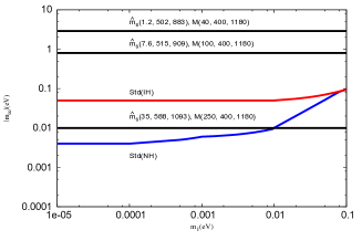
Figure 6: Variation of the effective mass parameters with lightest LH neutrino mass. The dominant non-standard contributions due to fermion singlet contributions are shown by three horizontal lines with corresponding mass values in GeV units. The subdominant effective mass parameters due to NH and IH cases shown are similar to the standard values.

7.2 Cancellation between effective mass parameters

When plotted as a function of singlet fermion mass eigen value $m_{S_{1}}$, the resultant effective mass parameter shows cancellation for certain region of the parameter space, the cancellation being prominent in the QD case. Like the light neutrino masses, the singlet fermion masses $m_{S_{i}}$ are also expected to have two Majorana phases. When all Majorana phases are absent, both in the light active neutrino as well as in the singlet fermion sectors, it is clear that in the sum of the two effective mass parameter there will be cancellation between light active neutrino and the singlet fermion contributions because of the inherent negative sign of the non-standard contribution. Our estimations for NH, IH, and QD patterns of light neutrino mass hierarchies are discussed separately.

A. Effective mass parameter for NH and IH active neutrino masses
In Fig. 7, we have shown the variation of the resultant effective mass parameter with $m_{S_{1}}$ for NH and IH patterns of active light neutrino masses. It is clear that for lower values of $m_{S_{1}}$, the singlet fermion exchange term continues to dominate. For larger values of $m_{S_{1}}$ the resultant effective mass parameter tends to be identical to the light neutrino mass contribution due to the vanishing non-standard contribution. We note that the values $|m_{eff}|=0.5-0.1$ eV can be easily realised for $|m_{S_{1}}|=3-5$ GeV in the NH case but for $|m_{S_{1}}|=1-2$ GeV in the IH case.

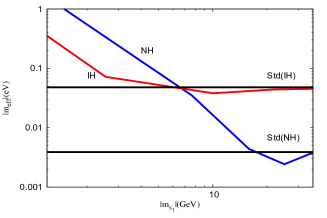
Figure 7: Variation of effective mass parameter of $0\nu\beta\beta$ decay with the mass of the lightest singlet fermion for $|p|=190$ MeV .

B. Effective mass parameter for QD neutrinos
The variation of effective mass with $m_{S_{1}}$ for the QD case with one experimentally determined Dirac phase $\delta=0.8\pi$ and assumed values of two unknown Majorana phases is given in Fig. 8. The upper-panel of Fig. 8 shows the variation with $\alpha_{1}=\alpha_{2}=0$ for different choices of the common light neutrino mass $m_{0}=0.5$ eV, $0.3$ eV , and $0.2$ eV for the upper, middle, and the lower curves, respectively, where cancellations are clearly displayed in the regions of $m_{s_{1}}=0.4-1.5$ GeV. However, before such cancellation occurs, the dominance of the singlet exchange contribution has been clearly shown to occur in the regions of lower values of $m_{S_{1}}$. For larger values of $m_{S_{1}}>5$ GeV, the singlet exchange contribution tends to be negligible and the light QD neutrino contribution to $m_{eff}$ is recovered. In the lower panel of Fig. 8, the upper curve corresponds to $\alpha_{1}=\pi$,$\alpha_{2}=\pi$ at $m_{0}=0.2eV$. The middle line corresponds to $\alpha_{1}=\pi$,$\alpha_{2}=0$ at $m_{0}=0.5eV$ .The lower line corresponds to $\alpha_{1}=0$,$\alpha_{2}=\pi$ at $m_{0}=0.3eV$. We find that because of introduction of appropriate Majorana phases the dips in two curves have disappeared.

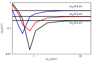
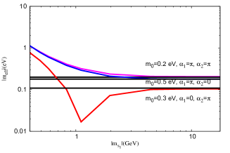
Figure 8: Variation of effective mass of $0\nu\beta\beta$ decay with the mass of the lightest singlet fermion for QD light neutrinos with one Dirac phase (left), and with one Dirac phase and two Majorana phases (right) .

7.3 Half-life as a function of singlet fermion masses

In order to arrive at a plot of half-life against the lightest singlet fermion mass in different cases, at first we estimate the mass eigen values of the three singlet fermions for different allowed combinations of the $N-S$ mixing matrix elements satisfying the non-unitarity constraint of eq.(43) and by using the RH neutrino mass matrices predicted for NH, IH, and QD cases from eq.(26), eq.(28), eq.(30), and eq.(31). These solutions are shown in Table 4.
We then derive expressions for half-life taking into account the contributions of the two different amplitudes or effective mass parameters arising out of the light neutrino and the singlet fermion exchanges leading to

$$\left[T_{1/2}^{0\nu}\right]=\frac{{m_{s1}^{2}}}{{K_{0\nu}}|p|^{4}{({M_{D}/M})_{e1}}^{4}}\bigg{[}|1+X+Y|\bigg{]}^{-2},$$ (63)

where

$$X = \frac{{{({M_{D}/M}})_{e2}}^{2}}{{{({M_{D}/M}})_{e1}}^{2}}\frac{m_{S_{1}}}{m_{s_{2}}}+\frac{{{({M_{D}/M}})_{e3}}^{2}}{{{({M_{D}/M}})_{e1}}^{2}}\frac{m_{S_{1}}}{m_{S_{3}}},$$ (64)

$$Y = {\bf m}^{ee}_{\nu}\frac{m_{S_{1}}}{p^{2}{(M_{D}/M)}_{e1}^{2}}.$$ (65)

Here we have used the expression for ${\bf m}^{ee}_{\nu}$ given in eq.(52). In eq.(63), $Y=0$ gives complete dominance of the singlet fermion exchange term. However this formula of half-life is completely different from the one obtained using inverse seesaw dominance in SO(10) [20]. In the present model in the leading order, the predicted half-life depends directly on the square of the lightest singlet fermion mass and it is independent of the RH neutrino mass which is non-diagonal. But in [20] , the half-life of neutrino less double beta decay is directly proportional to the fourth power of the lightest singlet fermion mass and square of the lightest right handed neutrino mass leading into a different result.

$M$	$\hat{m_{s}}(NH)$
(GeV)	(GeV)
(40,400,1180)	(1.2,502,883)
(100,400,1180)	(7.65,515,909))
(150,400,1180)	(16,533,951)
(200,400,1180)	(25,558,1011)
(250,400,1180)	(35,588,1093)
(300,400,1180)	(43,622,1200)
(350,400,1180)	(50,659,1331)

$M$	$\hat{m_{s}}(IH)$
(GeV)	(GeV)
(40,450,1280)	(0.4,54.32,7702)
(60,450,1280)	(0.9,54.4,7705)
(70,450,1280)	(1.2,54.4,7706)
(100,450,1280)	(2.5,55,7715)
(300,450,1280)	(22,56,7831)
(400,450,1280)	(36.2,59,7933)
(450,450,1280)	(42,64,7996)

$M$	$\hat{m_{s}}(QD)$
(GeV)	(GeV)
(100,600,1500)	(0.5,17.7,109))
(130,600,1500)	(0.8,17.7,109)
(200,600,1500)	(1.97,17.7,109)
(300,600,1500)	(4.4,17.7,109)
(350,600,1500)	(6.05,17.7,109)
(400,600,1500)	(8,17.7,109)
(500,600,1500)	(12.3,17.7,109)
(600,600,1500)	(17.7,17.7,109)

Table 4: Eigen values of singlet fermion masses for different allowed $N-S$ mixing matrix elements and for NH, IH, and QD patterns of light neutrino masses

A. Half-life in the NH and IH cases
We have computed the half-life for NH and IH patterns of active neutrino masses, taking the contributions of singlet fermion as well as light active neutrino exchanges. This is shown in the upper panel for NH case and in the lower panel for IH case in Fig.9. Taking both $X$ term and $Y$ term in eq.(63), we find that for smaller value of $m_{S_{1}}$, the contribution due to sterile neutrino is dominated for both NH and IH cases. But with the increase in the value of $m_{S_{1}}$, the half-lfe increases showing its decreasing strength. The predicted half-life curve saturates the experimental data at $m_{S_{1}}\simeq 3$ GeV and $m_{S_{1}}\simeq 2$ GeV for the NH and the IH cases, respectively. The interesting predictions are that if the lightest sterile neutrino mass satisfies the bound $m_{S_{1}}\leq 3GeV$, then the $0\nu\beta\beta$ decay should be detected with half-life close to the current experimental bound even if the light neutrino masses have NH pattern of masses. Similarly the corresponding bound for the IH case is $m_{S_{1}}\leq 2$ GeV. But in a recent paper[20] which has inverse seesaw dominant neutrino mass, the corresponding bound for the NH and IH case is $m_{S_{1}}\leq 14$ GeV.

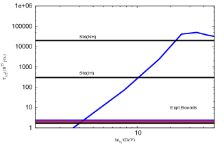
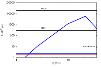
Figure 9: Variation of half-life of $0\nu\beta\beta$ decay with the sterile neutrino mass for NH(left) and IH(right) patterns of light active neutrino masses for $|p|=190$ MeV .

B. Lifetime prediction with QD neutrino masses.

For QD masses of light active neutrinos, we considered the $X$ term and $Y$ term of eq.(63) i.e including both the sterile neutrino exchange and light neutrino exchange contributions. For the light-neutrino effective mass parameter occuring in $Y$, we have considered three different cases with common light-neutrino mass values $m_{0}=0.2{\rm eV},0.3{\rm eV}$, and $0.5{\rm eV}$ resulting in three different curves shown in the upper- and the lower- panels of Fig. 10. In the upper-panel, only the experimentally determined Dirac phase $\delta=0.8\pi$ has been included in the PMNS mixing matrix for light QD neutrinos while ignoring the two Majorana phases($\alpha_{1}=\alpha_{2}=0$). In the lower-panel while keeping $\delta=0.8\pi$ for all the three curves, the Majorana phases have been chosen as indicated against each of them. As the sterile neutrino exchange amplitude given in eq.(53) is inversely proportional to the eigen value of the corresponding sterile neutrino mass $m_{S_{i}}$, even in the quasi-degenerate case this contribution is expected to dominate for allowed small values of $m_{S_{i}}$. This fact is reflected in both the figures given in Fig.10. When Majorana phases are ignored, this dominance gives half-life less than the current bounds for $m_{S_{1}}<0.5$ GeV when $m_{0}=0.5$ eV, but for $m_{S_{1}}<0.7$ GeV when $m_{0}=0.2-0.3$ eV. When Majorana phases are included preventing cancellation between the two contributions, these crossing points are changed to $m_{S_{1}}<0.7$ GeV when $m_{0}=0.3$ eV, but $m_{S_{1}}<1.0$ GeV when $m_{0}=0.2-0.5$ eV. Repeating the same procedure for ref. [20] which is based upon inverse seesaw dominance, the corresponding bound for the QD case is $m_{S_{1}}\leq 12.5$ GeV.

In the present case, the peaks in the half-life prediction appear because of cancellation between the two effective parameters. Inclusion of Majorana phases annuls cancellation resulting in constructive addition of the two effective mass parameters and reduced values of half-life accessible to ongoing searches. For larger values of $m_{S_{1}}>>20$ GeV, the sterile neutrino contribution to $0\nu\beta\beta$ amplitude becomes negligible and the usual contributions due to light quasi-degenerate neutrinos are recovered.

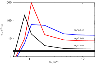
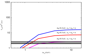
Figure 10: Variation of half-life of $0\nu\beta\beta$ decay with the mass of the lightest singlet fermion for QD light neutrinos including one Dirac phase (left curve) and one Dirac phase and two Majorana phases (right curve) .

8 Brief discussion on other aspects and leptogenesis

Here we discuss briefly constraints imposed on the model by electroweak precision observables and predictions on the order of magnitude of baryon asymmetry of the universe through resonant leptogenesis[65]. We also point out occurence of small $Z-Z^{\prime}$ mixings while indicating briefly a possible application for dilepton production. Since details of analyses and predictions on these aspects are beyond the scope of this paper, they will be presented elsewhere [57]

(a)Electroweak precision observables and other constraints
We have shown that dominant contributions to $0\nu\beta\beta$ decay are possible for the first generation sterile neutrino masses ${\hat{m}}_{S_{1}}\sim{\mathcal{O}}(1)$ GeV. For larger values of this mass ${\hat{m}}_{S_{1}}\sim 5-10$ GeV partial cancellation between effective mass parameters due to light neutrino and sterile neutrino exchanges occurs depending upon choices of different Majorana phases. Different lighter sterile mass eigen values relevant for $0\nu\beta\beta$ decay are shown in Table 4 in the NH, IH, and QD cases. It is pertinent to discuss influence of these lighter masses on the precision electroweak observables.
For choices of parameters permitted by observable LFV and/or dominant LNV, the sterile fermion masses of the first two generations could be ${\hat{m}}_{s_{i}}<45$ GeV ,$i=1,2$ whereas in the absence of dominant LNV decay, the mass eigen values could be even larger ${\hat{m}}_{s_{i}}\simeq 500$ GeV. When they are in the range of $1-45$ GeV, we have estimated the corresponding corrections on electroweak observables. The $\nu-S$ mixing ${\mathcal{V}}^{\nu S}=({M_{D}\over M})_{\nu S}$ is well determined in our model and all the relevant $\nu-S$ mixings are easily deduced using eq.(36) and eq.(43). In the allowed kinematical region, we have estimated the partial decay widths,

$$\Gamma(Z\to S_{i}S_{i})=\Gamma^{\nu{\bar{\nu}}}_{Z}[\sum_{\alpha}|\left(\mathcal{V}^{\nu S}_{\alpha,i}\right)|^{4}]\,(i=1,2),$$ (66)

where the standard value $\Gamma^{\nu{\bar{\nu}}}_{Z}=0.17$ GeV and $\mathcal{V}^{\nu S}_{\alpha,i}=(M_{D}/M)_{\alpha,i}$ with $\alpha=\nu_{e},\nu_{\mu},\nu_{\tau}$ and $i=1,2,3$. We then obtain $\Gamma(Z\to S_{1}S_{1})=1.2\times 10^{-14}$ GeV for NH, IH, and QD cases, and $\Gamma(Z\to S_{2}S_{2})=6.6\times 10^{-11}$ GeV for QD case only. Similarly we have estimated the partial decay width

$$\Gamma(W\to lS_{i})=\Gamma^{l{\nu}}_{W}[\sum_{\alpha}|\left(\mathcal{V}^{\nu S}_{\alpha,i}\right)|^{2}]\,(i=1,2),$$ (67)

and obtained $\Gamma(W\to eS_{1})\simeq\Gamma(W\to eS_{2})=3.5\times 10^{-9}$ GeV, $\Gamma(W\to\mu S_{1})\simeq\Gamma(W\to\mu S_{2})=1.8\times 10^{-7}$ GeV, and $\Gamma(W\to\tau S_{1})\simeq\Gamma(W\to\tau S_{2})=1.0\times 10^{-5}$ GeV. These and other related estimations cause negligible effects on electroweak precision observables [58] primarily because of small $\nu-S$ mixings determined by the model analyses. In addition to these insignificant tree level corrections, new physics effects may affect the electroweak observables indirectly via oblique corrections through loops leading corrections to the Peskin-Takeuchi $S,T,U$ parameters [59, 60]. Although the computation of these loop effects are beyond the scope of the present paper, it may be interesting to estimate how the new fermions through their small mixings with active neutrinos may affect the leptonic and the invisible decay widths of the Z-boson, the W-mass, and other observables [57].

In this model the neutral generator corresponding to heavy $Z^{\prime}$ is a linear combinations of $U(1)_{R}$ and $U(1)_{B-L}$ generators while the other orthogonal combination is the $U(1)_{Y}$ generator of the SM [16, 33]. The $Z-Z^{\prime}$ mixing in such theories is computed through the generalised formula $\tan^{2}{\theta_{zz^{\prime}}}=\frac{M_{0}^{2}-M_{Z}^{2}}{M_{Z^{\prime}}^{2}-M_{0}^{2}}$ where $M_{0}=\frac{M_{W}}{{\sqrt{\rho}_{0}}\cos\theta_{W}}$. In our model since the LH triplet $\Delta_{L}(3,-1,1)$ has a very small VEV $v_{L}=0.1-0.5$ eV $<<V_{\rm ew}$, the model is consistent with the tree level value $\rho_{0}=1$. The radiative corrections due to the $125$ GeV Higgs of the SM and the top quark yield $\rho\simeq 1.009$ [61]. The new neutral gauge boson $Z^{\prime}$ in principle may have additional influence on the electroweak precision parameters as well as the $Z-$pole parameters if $M_{Z^{\prime}}<<{\cal O}(1)$ TeV [33, 67]. The most recent LHC data has given the lower bound $M_{Z^{\prime}}\geq 1.6$ TeV [63]. Since our model is based on extended seesaw mechanism, we require $V_{R}>>V_{ew}=246$ GeV and this implies $M_{Z^{\prime}}>>M_{Z}$ but accessible to LHC. Under this constraint $M_{Z^{\prime}}\sim{\cal O}(5-10)$ TeV are the most suitable predictions of both the models discussed in this work. As some examples, using such values of $M_{Z^{\prime}}$ and the most recently reported values from Particle Data Group [62] of $\sin^{2}\theta_{W}=0.23126\pm 0.00005$, $M_{W}=80.385\pm 0.015$GeV, $M_{Z}=91.1876\pm 0.0021$ GeV, $\rho_{0}=1.01$, we obtain $\theta_{zz^{\prime}}=0.00131\pm 0.0003,\,\,0.0005\pm 0.00012,\,\,0.0003\pm 0.00008$,   and $0.0002\pm 0.00006$ for $M_{Z^{\prime}}=2.0{\rm TeV},\,\,5.0{\rm TeV},\,\,7.5{\rm TeV}$,   and $10{\rm TeV}$ ,respectively. Because of the smallness of the values, these mixings are consistent with the electroweak precision observables including the $Z-$ pole data [33, 67, 68]. Some of these masses may be also in the accessible range of the ILC [69]. Details of experimental constraints on $Z-Z^{\prime}$ mixings as a function of $Z^{\prime}$ masses would be investigated elsewhere [57].

(b)Possibility of dilepton signals at LHC
In both the models considered in this work, there are two types of heavy Majorana neutrinos: (i) the RH neutrinos with masses $M_{N_{i}}\geq{\cal O}(1-10)$ TeV, (ii) some of the three sterile neutrinos with masses ${\hat{m}}_{S-i}<<M_{N_{i}}$. In principle both of these classes of fermions are capable of contributing to dilepton production at LHC through the sub-processes $pp\to W^{\pm}_{L}\to l^{\pm}l^{\pm}jjX$ where, for example, the $W_{L}^{+}$ produced from $pp$ collision gives rise to a charged lepton $l^{+}$ and a $N_{i}$ or $S_{i}$ in the first step by virtue of the latters’ mixing with the charged leptons given in eq.(39). The particle $N_{i}$ or $S_{i}$ can then produce a second charged lepton of the same sign and a $W^{-}_{L}$ boson that is capable of giving rise to two jets. It is interesting to note that our model predicts a rich structure of like sign dilepton production through the mediation of $N_{i}$ or $S_{i}$, or both. From details of model parametrisations discussed in Sec.3-Sec.5, we have found the corresponding mixing matrices with charged leptons defined through eq.(39) discussed in Sec.5. We have estimated the elements ${\cal V}^{\nu N}_{e1}\simeq-0.0000727+i0.000203$ and ${\cal V}^{\nu N}_{\mu 2}\simeq 0.000813-i0.001148$ which would contribute to the production cross sections of $pp\to e^{\pm}e^{\pm}jjX$ and $pp\to\mu^{\pm}\mu^{\pm}jjX$ by the exchange of RH neutrinos, the cross sections being proportional to the modulus squares of these mixings. Similarly we have ${\cal V}^{\nu S}_{\mu 2}\simeq 0.0003191$ which can also contribute to production process $pp\to\mu^{\pm}\mu^{\pm}jjX$ by the exchange of the second sterile neutrino mass eigen state. The first sterile neutrino is too light to mediate the dilepton production process. Thus the LHC evidence of dilepton production signals, may indicate the presence of heavy Majorana neutrinos [56]. Details of predictions will be reported elsewhere [57].

(c)Leptogenesis
This model may have a wider range of possibilities for leptogenesis via decays of Higgs triplets [64], or through the decays of LHC scale Majorana fermions $N$ or $S$. Although rigorous estimation including solutions of Boltzmann equations is beyond the scope of this work which will be addressed elsewhere[57], we discuss here briefly only a plausible case with a very approximate estimation of the CP asymmetry parameter and the order of magnitude of the baryon asymmetry through the decays of two nearly degenerate Majorana masses of sterile neutrinos. For resonant leptogenesis through the decays of a pair of quasi-degenerate RH neutrinos, relevant formulas for CP-asymmetry and baryon asymmetry have been suggested in [65]. Noting that ${\hat{m}}_{S_{1}}\sim{\mathcal{O}}(1)$ GeV is important for dominant contribution to $0\nu\beta\beta$ decay and the $N-S$ mixing matrix elements $M_{2}\sim M_{3}\simeq{\mathcal{O}}(1)$ TeV are capable of predicting experimentally accessible LFV decays in our model, we choose an interesting region of the parameter space $M\simeq{\rm diag.}(146,3500,3500)$ GeV in the quasi-degenerate case of $S_{2}$ and $S_{3}$. Then using the $G_{2113}$ breaking VEV $V_{R}\simeq{\mathcal{O}}(10)$ TeV, the results of Sec. 3.3 in the QD case of active neutrinos, and eq.(14) we obtain

$${\hat{m}}_{S_{i}} = {\rm diag.}(1.0,595.864..,595.864..){\rm GeV}.$$ (68)

where ellipses on the RHS indicate higher degree of quasi-degeneracy of the two masses the model tolerates. In order to estimate lepton asymmetry caused by the decay of heavy sterile fermions ${\hat{S}}_{k}(k=2,3)$ via their mixing with the heavier RH neutrinos, the corresponding Feynmann diagrams at the tree and one-loop levels, including the vertex and self energy diagrams, are shown in Fig. 11.

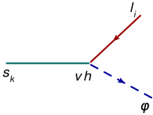
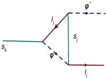
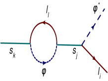
Figure 11: Tree and one-loop diagrams for the $S_{k}$ decay contributing to the CP-asymmetry. All fermion-Higgs couplings in the diagrams are of the form $Vh$ where $h=N-l-\Phi$ Yukawa coupling and $V\simeq M/M_{N}$.

The fermion Higgs coupling in all the diagrams is $Vh$ instead of the standard Higgs-Yukawa coupling $h=M_{D}/V_{\rm wk}$ where ${\mathcal{V}}\simeq{M/M_{N}}$, $M_{D}$ is given in eq.(36), and $V_{\rm wk}\simeq 174$ GeV. The widths of these sterile fermion are $\Gamma_{S_{2}}\simeq 16.3\,\,{\rm keV}$ and $\Gamma_{S_{3}}\simeq 14.0\,\,{\rm MeV}$. In order to exploit quasidegeneracy of the second and the third generation fermions in resonant leptogenesis, we use the formula for CP asymmetry generated due to interference between the tree and the self energy graphs [65],

$$\varepsilon_{S_{k}} = \sum_{j}\frac{{\cal I}m[(y^{\dagger}y)_{kj}^{2}]}{|y^{\dagger}y|_{jj}|y^{\dagger}y|_{kk}}R$$

$$R = \frac{({\hat{m}}_{S_{i}}^{2}-{\hat{m}}_{S_{j}}^{2}){\hat{m}}_{S_{i}}\Gamma_{S_{j}}}{({\hat{m}}_{S_{i}}^{2}-{\hat{m}}_{S_{j}}^{2})^{2}+{\hat{m}}_{S_{i}}^{2}\Gamma_{S_{j}}^{2}}\,,$$ (69)

where $y=M/M_{N}h$, $h=M_{D}/V_{\rm wk}$ ,and $V_{\rm wk}\simeq 174$ GeV. For computation of the baryon asymmetry $Y_{B}$ with a given washout factor $K$, we have also utilised the suggested formula[65]

$$Y_{B} \simeq \frac{\varepsilon_{S_{k}}}{200K_{k}},$$

$$K_{k} = \frac{\Gamma_{S_{k}}}{H({\hat{m}}_{S_{k}})},$$ (70)

$H({\hat{m}}_{S_{k}})$ being the Hubble parameter at temperature ${\hat{m}}_{S_{k}}$. As in TeV scale leptogenesis models, here also we encounter large wash-out factors which, in some cases, tend to damp out the baryon asymmetry generation. However it has been shown [66] that all the $\Delta L=2$ processes, $l\Phi\to{\bar{l}}\Phi^{\dagger}$ expected to cause the most dominant washouts are substantially depleted for the heavier quasidegenerate Majorana masses of the decaying fermions. The depletion factor is proportional to $\delta_{i}^{2}$ leading to an effective washout factor $K_{i}^{\rm eff}$ that replaces $K_{i}$ for the $i-$th decaying Majorana fermion

$$\delta_{i} = \frac{|{\hat{m}}_{S_{i}}-{\hat{m}}_{S_{j}}|}{\Gamma_{S_{i}}}(i\neq j),$$

$$K_{i}^{\rm eff} \simeq \delta_{i}^{2}K_{i}.$$ (71)

We find sizeable baryon asymmetry in the following two cases: (i)In the case of finite perturbation theory, the ${\hat{m}}_{S_{j}}^{2}\Gamma_{S_{j}}^{2}$ term in the denominator of $R$ has been noted to be absent[65] leading to a singular term in the CP-asymmetry. (ii)In the limit when $|{\hat{m}}_{S_{i}}-{\hat{m}}_{S_{j}}|<<\Gamma_{S_{j}}/2$, $R=2{({\hat{m}}_{S_{i}}-{\hat{m}}_{S_{j}})\over\Gamma_{S_{j}}}$.

(i)Finite perturbation theory

$$R = {1\over 2}\frac{\Gamma_{j}}{({\hat{m}}_{S_{j}}-{\hat{m}}_{S_{k}})},$$

$$\delta_{jk} = (1-{{\hat{m}}_{S_{j}}\over{\hat{m}}_{S_{k}}}),$$

$$\varepsilon_{S_{k}} = \sum_{j}\frac{{\cal I}m[(y^{\dagger}y)_{kj}^{2}]}{16\pi|y^{\dagger}y|_{kk}\delta_{jk}}.$$ (72)

Similar formulas have been used by a number of authors in the case of decays of quasi-degenerate RH neutrinos [71] and, specifically, in the context of $SO(10)$[70]. For the decay of $S_{2}$ for which $K_{2}=2.7\times 10^{7}$, using $({\hat{m}}_{S_{2}}-{\hat{m}}_{S_{3}})\simeq 2\times 10^{-7}$ GeV, we obtain

$$\varepsilon_{S_{2}} = 0.824,$$

$$Y_{B} = 1.5\times 10^{-10}.$$ (73)

The fine tuning in the quasidegenerate masses can be reduced by one order if we use the effective wash out factor. For example using $({\hat{m}}_{S_{2}}-{\hat{m}}_{S_{3}})\simeq 1.35\times 10^{-6}$ GeV, we get $\delta_{2}=0.008$ leading to

$$\varepsilon_{S_{2}} = 0.0357,$$

$$K_{2}^{\rm eff} = 1.92\times 10^{5},$$

$$Y_{B} = 9.3\times 10^{-10}.$$ (74)

For the decay of $S_{3}$ for which $K_{3}=2.4\times 10^{10}$, using $({\hat{m}}_{S_{2}}-{\hat{m}}_{S_{3}})\simeq 10^{-6}$ GeV, we obtain $\delta_{3}^{2}\simeq 5\times 10^{-8}$, leading to

$$\varepsilon_{S_{3}} = 8\times 10^{-5},$$

$$K_{3}^{\rm eff} = 575.4,$$

$$Y_{B} = 7.3\times 10^{-10}.$$ (75)

(ii)Larger width limit :$\Gamma_{k}>2|({\hat{m}}_{S_{k}}-{\hat{m}}_{S_{j}})|$

$$R \simeq \frac{2({\hat{m}}_{S_{k}}-{\hat{m}}_{S_{j}})}{\Gamma_{k}},$$

$$\times\left[1+\frac{4({\hat{m}}_{S_{k}}-{\hat{m}}_{S_{j}})^{2}}{\Gamma_{k}^{2}}\right]^{-1},$$

$$\varepsilon_{S_{k}} = \sum_{j}\frac{{\cal I}m[(y^{\dagger}y)_{kj}^{2}]}{8\pi|y^{\dagger}y|_{kk}\Gamma_{k}}{\hat{m}}_{S_{k}}R.$$ (76)

This case can be more efficiently implemented for $S_{3}$ decay which has $\Gamma_{S_{3}}\simeq 14$ MeV, and $K_{3}=2.4\times 10^{11}$. In this case the depletion in $K_{3}$ is quite effective. Using $({\hat{m}}_{S_{2}}-{\hat{m}}_{S_{3}})\simeq 10^{-6}$ GeV, we obtain $\delta_{3}^{2}\simeq 5\times 10^{-11}$, leading to

$$\varepsilon_{S_{3}} = 3\times 10^{-7},$$

$$K_{3}^{\rm eff} = 10.3,$$

$$Y_{B} = 1.1\times 10^{-10}.$$ (77)

Thus we have shown very approximately that the model may be capable of accommodating the order of magnitude of baryon asymmetry of the universe that requires fine tuning of the mass difference of the two sterile neutrino in the range $10^{-6}-10^{-7}$ GeV. In a separate paper we plan to look into improvement in these approximate solutions and other possible channels of leptogenesis including the impact of the present model on electroweak precision observables and detection possibilities of RH neutrinos, $S-$ fermions, and the $Z^{\prime}$ at collider energies such as LHC and ILC[57].

9 Summary and conclusion

In this work we have investigated the prospect of having a new type-II seesaw dominated neutrino mass generation mechanism in non-SUSY $SO(10)$ GUT by a novel procedure by introducing one additional singlet fermion per generation. Following the popular view that the only meaningful fermion masses in the Lagrangian must have dynamical origins, and taking the non-dynamical singlet fermion mass $\mu_{S}$ to be negligible, one of the models (Model-I) discussed is found to exhibit type-II seesaw dominance and it predicts TeV scale $Z^{\prime}$ boson accessible to LHC without any drastic fine tuning in the corresponding Yukawa sector. For Model-II the desired type-II seesaw dominance requires an additional fine tuning upto one part in a million. The would be dominant type-I seesaw contribution to neutrino masses in both models cancels out. The induced contribution to the $\nu-S$ mixing mass term $M_{L}$ is shown to be damped out because of the GUT-scale mass of the LH doublet in ${16}_{H}$ that renders the linear seesaw contribution to light neutrino masses naturally negligible in the Model-I, although in Model-II it needs additional fine tuning. In spite of the high values of the type-II seesaw scale $M_{\Delta_{L}}\simeq 10^{8}-10^{9}$ GeV $>>M_{Z}$, the models predict new dominant contributions to $0\nu\beta\beta$ decay in the $W_{L}-W_{L}$ channel mediated by sterile neutrinos which acquire Majorana masses. The predicted LFV decay branching ratios for $\mu\to e\gamma$, $\tau\to\mu\gamma$, and $\tau\to e\gamma$, are found to be accessible to ongoing and planned experiments. We discuss the impact on the resultant effective mass parameter and $0\nu\beta\beta$ half-life showing cancellation between light-neutrino exchange and sterile neutrino exchange contributions. The cancellation occurs because of the opposite signatures of the two effective mass parameters due to light neutrino exchange and the sterile neutrino exchange when effects of Majorana phases are ignored. We derive an analytic formula for the half-life of $0\nu\beta\beta$ decay as a function of singlet fermion masses which predicts a lower bound on the lightest sterile neutrino mass eigen value from the current experimental data on lower bounds. We find that the half-life close to the current lower bound or even lower can be easily accommodated even with NH or IH patterns of light neutrino masses . We find that the QD nature of light neutrino masses is not a necessary criteria to satisfy existing lower bounds on the half life estimated by different experimental groups. Even if the light active neutrino masses are NH or IH, a half-life prediction $T_{1/2}\simeq(2-5)\times 10^{25}$ yrs is realizable if the lightest sterile neutrino mass $m_{S_{1}}\simeq 2-3$ GeV. Depending upon the common mass of the light QD neutrinos, the model also predicts lifetime $T_{1/2}\leq 2\times 10^{25}$ yrs for $m_{S_{1}}\leq(0.5-1.0)$ GeV. Large cancellation between the two contributions is found to occur in the quasidegenerate case of light active neutrinos in the regions of sterile neutrino mass $m_{S_{1}}\simeq 2-8$ GeV. The bounds obtained in the sterile neutrino mass in these type-II seesaw dominant models are significantly smaller than that of the bounds obtained in the inverse seeseaw model [20]. As the sterile neutrino contribution to the $0\nu 2\beta$ decay is inversely proportional to the corresponding mass eigen values, the smallness of the lightest mass eigen values causes dominant contributions compared to those by light neutrinos in NH, IH, and QD cases. For the same reason the new contributions are damped out for large sterile neutrino mass eigen values. Because of the underlying type-II seesaw formula for neutrino masses, heavy RH neutrino masses in the range ${\mathcal{O}}(100)$ GeV-${\mathcal{O}}(10000)$ GeV and with specified heavy-light neutrino mixings are also predicted which can be testified at the LHC and future high energy accelerators. The proton lifetime predictions for $p\to e^{+}\pi^{0}$ for some regions of the parameter space are also accessible to ongoing experimental searches especially for intermediate mass values of the color octet scalar which has been found to be necessary for gauge coupling unification. Further we have verified that the lighter $S_{1}$ or $S_{2}$ states in the models have negligible effects on values of electroweak precision observables at the tree level although loop effects through Peskin-Takeuchi parameters $S,T,U$ will be investigated elsewhere. Approximate estimations show occurence of small $Z-Z^{\prime}$ mixings apparently consistent with $Z-pole$ and non-$Z-pole$ data. The possibility of dilepton signals at LHC in the $W_{L}-W_{L}$ channel is briefly noted in both the models while an approximate estimation indicates possibility of baryon asymmetry generation through leptogenesis due to decay of quasidegenerate sterile Majorana fermions at the TeV scale. The details and rigorous estimations on dilepton signals, leptogenesis, estimation of $S,T,U$ parameters, and the impact of $Z-Z^{\prime}$ mixings on $Z-pole$ and non-$Z$ pole data including electroweak precision observables are currently under investigation and would be reported separately[57].

Acknowledgment
M. K. P. thanks Thomas Hambye for discussion and the Department of Science and Technology, Govt. of India for the research project, SB/S2/HEP-011/2013. B. N. thanks Siksha ’O’ Anusandhan University for a research fellowship.

9.1 Appendix A

Beta function coefficients for RG evolution of gauge couplings
The renormalisation group equations for gauge couplings are

$$\mu{\partial g_{i}\over{\partial\mu}}=\frac{a_{i}}{16\pi^{2}}g_{i}^{3}+\frac{1}{(16\pi^{2})^{2}}\sum_{j}b_{ij}g_{i}^{3}g_{j}^{2},$$ (78)

where $a_{i}$($b_{ij}$) are one-(two-)loop beta function coefficients. Their values for the Model-I and Model-II are given in Table 5.

$Symmetry$	${a_{i}}$	${b_{ij}}$
		(GeV)
$G_{213}$	$\begin{pmatrix}-19/6,41/10,-7\end{pmatrix}$	$\begin{pmatrix}199/50,27/10,44/5\\ 9/10,35/6,12\\ 11/10,9/2,-26\end{pmatrix}$
$G_{2113}$	$\begin{pmatrix}-3,57/12,37/8,-7\end{pmatrix}$	$\begin{pmatrix}8,1,3/2,12\\ 3/2,33/57,63/8,12\\ 9/2,63/8,209/16,4\\ 9/2,3/2,1/2,26\end{pmatrix}$
$G_{2213}$	$\begin{pmatrix}-2,-3/2,29/4,-7\end{pmatrix}$	$\begin{pmatrix}31,6,39/2,12\\ 6,115/6,3/2,12\\ 81/2,6,181/8,4\\ 9/2,9/2,1/2,-26\end{pmatrix}$
$G_{2213D}$	$\begin{pmatrix}-3/2,-3/2,15/2,-7\end{pmatrix}$	$\begin{pmatrix}319/6,6,57/4,12\\ 6,319/6,57/4,12\\ 171/4,171/4,239/4,4\\ 9/2,9/2,1/2,-26\end{pmatrix}$

Table 5: One-loop and two-loop beta function coefficients for gauge coupling evolutions described in the text taking the second Higgs doublet mass at $1$ TeV

9.2 Appendix B

Block diagonalisation and determination of $\cal{M}_{\nu}$
In this section we discuss the various steps of block diagonalisation in order to calculate the light neutrino mass , sterile neutrino mass and right-handed neutrino mass and their mixings. The complete $9\times 9$ mass matrix in the flavor basis $\{\nu_{L},S_{L},N^{C}_{R}\}$ is

$$\mathcal{M}=\begin{pmatrix}m_{\nu}^{II}&M_{L}&M_{D}\\ M_{L}^{T}&0&M\\ M_{D}^{T}&M^{T}&M_{N}\end{pmatrix}$$ (79)

, where $M_{L}=y_{\chi}v_{\chi_{L}}$, $M=y_{\chi}v_{\chi_{R}}$, $M_{N}=fv_{R}$
and $M_{D}$ is the Dirac neutrino mass matrix as discussed in Sec.4.
Assuming a generalized unitary transformation from mass basis to flavor basis, gives

$$|\psi\rangle_{flavor}=\mathcal{V}\,|\psi\rangle_{mass}$$ (80)

or

$$\,\begin{pmatrix}\nu_{\alpha}\\ S_{\beta}\\ N^{C}_{\gamma}\end{pmatrix}=\begin{pmatrix}{\cal V}^{\nu\nu}_{\alpha i}&{\cal V}^{\nu{S}}_{\alpha j}&{\cal V}^{\nu{N}}_{\alpha k}\\ {\cal V}^{S\nu}_{\beta i}&{\cal V}^{SS}_{\beta j}&{\cal V}^{SN}_{\beta k}\\ {\cal V}^{N\nu}_{\gamma i}&{\cal V}^{NS}_{\gamma j}&{\cal V}^{NN}_{\gamma k}\end{pmatrix}\begin{pmatrix}\hat{\nu}_{i}\\ \hat{S}_{j}\\ \hat{N}_{k}\end{pmatrix}$$ (81)

with

$$\,\mathcal{V}^{\dagger}\mathcal{M}\mathcal{V}^{*}=\hat{\mathcal{M}}={\rm diag}\left({\hat{\mathcal{M}}}_{\nu_{i}};{\hat{\mathcal{M}}}_{{\cal S}_{j}};{\hat{\mathcal{M}}}_{{\cal N}_{k}}\right)$$ (82)

Here $\mathcal{M}_{\nu}$ is the $9\times 9$ neutral fermion mass matrix in flavor basis with $\alpha,\beta,\gamma$ running over three generations of light-neutrinos, sterile-neutrinos and right handed heavy-neutrinos in their respective flavor states and $\hat{\mathcal{M}}_{\nu}$ is the diagonal mass matrix with $(i,j,k=1,2,3)$ running over corresponding mass states .
In the first step of block diagonalisation, the full neutrino mass matrix is reduced to a block diagonal form $\hat{\mathcal{M}}_{\rm\tiny BD}$ and in the second step we further block diagonalize to obtain the three matrices as three different block diagonal elements, $\mathcal{M}_{\rm\tiny BD}$= $diag({\mathcal{M}_{\nu}},{m_{S}},{m_{N}})$ whose each diagonal element is a $3\times 3$ matrix.In our estimation, we have used the mass hierarchy $M_{N}>M\gg M_{D},M_{L},fv_{L}$. Finally in the third step we discuss complete diagonalization to arrive at the physical masses and their mixings.

9.2.1 Determination of $\mathcal{M}_{\rm\tiny BD}$

With two unitary matrix transformations $\mathcal{Q}_{1}$ and $\mathcal{Q}_{2}$,

$$\mathcal{Q}^{\dagger}\mathcal{M}_{\nu}\mathcal{Q}^{*}=\hat{\mathcal{M}}_{\rm\tiny BD},\mbox{}\quad$$ (83)

where

$$\mathcal{Q}=\mathcal{Q}_{1}\,\mathcal{Q}_{2}$$ (84)

i.e the product matrix $\mathcal{Q}=\mathcal{Q}_{1}\,\mathcal{Q}_{2}$ directly give $\mathcal{M}_{\rm\tiny BD}$ from $\mathcal{M}_{\nu}$ Here $\hat{\mathcal{M}}_{\rm\tiny BD}$, and $\mathcal{M}_{\rm\tiny BD}$ are the intermediate block-diagonal, and full block-diagonal mass matrices, respectively,

$$\hat{\mathcal{M}}_{\rm\tiny BD}=\begin{pmatrix}{\cal M}_{eff}&0\\ 0&{m_{N}}\end{pmatrix}$$ (85)

and

$$\,\mathcal{M}_{\rm\tiny BD}=\begin{pmatrix}{\cal M_{\nu}}&0&0\\ 0&{m_{S}}&0\\ 0&0&{m_{N}}\end{pmatrix}$$ (86)

9.2.2 Determination of $Q_{1}$

In the leading order parametrization the standard form of $\mathcal{Q}_{1}$ is

$$\mathcal{Q}_{1}=\begin{pmatrix}1-\frac{1}{2}R^{*}R^{T}&R^{*}\\ -R^{T}&1-\frac{1}{2}R^{T}R^{*}\end{pmatrix}\,,$$ (87)

where $R$ is a $6\times 3$ dimensional matrix.

$$R^{\dagger}=M_{N}^{-1}\left(M^{T}_{D},M^{T}\right)=(K^{T},J^{T})$$ (88)

$$J=M{M_{N}}^{-1}K=M_{D}M_{N}^{-1}I=KJ^{-1}=M_{D}M^{-1}$$ (89)

Therefore, the transformation matrix $\mathcal{Q}_{1}$ can be written purely in terms of dimensionless parameters $J$ and $K$

$$\mathcal{Q}_{1}=\begin{pmatrix}1-\frac{1}{2}KK^{\dagger}&-\frac{1}{2}KJ^{\dagger}&K\\ -\frac{1}{2}JK^{\dagger}&1-\frac{1}{2}JJ^{\dagger}&J\\ -K^{\dagger}&-J^{\dagger}&1-\frac{1}{2}(K^{\dagger}K+J^{\dagger}J)\end{pmatrix}$$ (90)

while the light and heavy mass matrices are

$${\cal M}_{eff} = \begin{pmatrix}fv_{L}&M_{L}\\ M_{L}^{T}&0\end{pmatrix}-\begin{pmatrix}M_{D}M_{N}^{-1}M_{D}^{T}&M_{D}M_{N}^{-1}M\\ M^{T}M_{N}^{-1}M^{T}_{D}&M^{T}M_{N}^{-1}M\end{pmatrix}$$ (91)

$${m_{N}} = M_{N}+..$$ (92)

Denoting

$${\cal M}_{eff} = \begin{pmatrix}Z&B\\ C&D\end{pmatrix}$$ (93)

,

$$Z=fv_{L}-M_{D}M_{N}^{-1}M_{D}^{T},$$ (94)

$$B=M_{L}-M_{D}M_{N}^{-1}M,$$ (95)

$$C=M_{L}^{T}-M^{T}M_{N}^{-1}M^{T}_{D},$$ (96)

$$D=M^{T}M_{N}^{-1}M,$$ (97)

9.2.3 Determination of $\mathcal{Q}_{2}$

The remaining mass matrix ${\cal M}_{eff}$ can be further block diagonalized using another transformation matrix

$$\mathcal{S}^{\dagger}\mathcal{M}_{\rm eff}\mathcal{S}^{*}=\begin{pmatrix}{\cal M_{\nu}}&0\\ 0&{m_{S}}\end{pmatrix}$$ (98)

such that in eq.(9.2.1)

$$\mathcal{Q}_{2}=\begin{pmatrix}\mathcal{S}&0\\ 0&1\end{pmatrix}$$ (99)

$$S=\begin{pmatrix}1-\frac{1}{2}P^{*}P^{T}&P^{*}\\ -P^{T}&1-\frac{1}{2}P^{T}P^{*}\end{pmatrix}$$ (100)

Using eq.(100) in eq.(98) ,we get through eq.(93)-eq.(97),

$$P^{\dagger} = (M^{T}M_{N}^{-1}M)^{-1}\left(M^{T}M_{N}^{-1}M^{T}_{D}-M^{T}_{L}\right)$$ (101)

$$= M^{-1}M_{D}^{T}-M^{-1}M_{N}M^{-1}M_{L}$$

where we have used $y_{\chi}$ to be symmetric. leading to

$${\mathcal{M}_{\nu}}=m_{\nu}^{II}+\left(M_{D}M_{N}^{-1}M^{T}_{D}\right)$$

$$-(M_{D}M_{N}^{-1}M^{T}_{D})+M_{L}(M^{T}M_{N}^{-1}M)^{-1}M_{L}^{T}$$

$$-M_{L}(M^{T}M_{N}^{-1}M)^{-1}(M^{T}M_{N}^{-1}M_{D}^{T})$$

$$-(M_{D}M_{N}^{-1}M)(M^{T}M_{N}^{-1}M)^{-1}M_{L}^{T},$$

$${m_{S}}=-MM_{N}^{-1}M^{T}+....,$$

The $3\times 3$ block diagonal mixing matrix $\mathcal{Q}_{2}$ has the following form

$$\mathcal{Q}_{2}=\begin{pmatrix}S&{\bf 0}\\ {\bf 0}&{\bf 1}\end{pmatrix}=\begin{pmatrix}1-\frac{1}{2}II^{\dagger}&I&0\\ -I^{\dagger}&1-\frac{1}{2}I^{\dagger}I&0\\ 0&0&1\end{pmatrix}$$ (103)

where we have used eq.(89) to define $I=KJ^{-1}=M_{D}M^{-1}$.
Complete diagonalization and physical neutrino masses
The $3\times 3$ block diagonal matrices $\cal{M}_{\nu}$, $m_{S}$ and $m_{N}$ can further be diagonalized to give physical masses for all neutral leptons by a $9\times 9$ unitary matrix $\mathcal{U}$ as

$$\mathcal{U}=\begin{pmatrix}U_{\nu}&0&0\cr 0&U_{S}&0\cr 0&0&U_{N}\end{pmatrix}.$$ (104)

where the $3\times 3$ unitary matrices $U_{\nu}$, $U_{S}$ and $U_{N}$ satisfy

$$U^{\dagger}_{\nu}\,{\cal M_{\nu}}\,U^{*}_{\nu} = \hat{\cal M_{\nu}}=\text{diag}\left({\cal M_{\nu}}_{1},{\cal M_{\nu}}_{2},{\cal M_{\nu}}_{3}\right)\,,$$

$$U^{\dagger}_{S}\,{m_{S}}\,U^{*}_{S} = \hat{m_{S}}=\text{diag}\left({m_{S}}_{1},{m_{S}}_{2},{m_{S}}_{3}\right)\,,$$

$$U^{\dagger}_{N}\,{m_{N}}\,U^{*}_{N} = \hat{m_{N}}=\text{diag}\left({m_{N}}_{1},{m_{N}}_{2},{m_{N}}_{3}\right)\,$$ (105)

With this discussion, the complete mixing matrix is

$$\mathcal{V}=\mathcal{Q}\cdot\mathcal{U}=\left(\mathcal{Q}_{1}\cdot\mathcal{Q}_{2}\cdot\mathcal{U}\right)$$

$$=\begin{pmatrix}1-\frac{1}{2}KK^{\dagger}&-\frac{1}{2}KJ^{\dagger}&K\\ -\frac{1}{2}JK^{\dagger}&1-\frac{1}{2}JJ^{\dagger}&J\\ -K^{\dagger}&-J^{\dagger}&1-\frac{1}{2}(K^{\dagger}K+J^{\dagger}J)\end{pmatrix}\cdot$$

$$\begin{pmatrix}1-\frac{1}{2}II^{\dagger}&I&0\\ -I^{\dagger}&1-\frac{1}{2}I^{\dagger}I&0\\ 0&0&1\end{pmatrix}\begin{pmatrix}U_{\nu}&0&0\\ 0&U_{S}&0\\ 0&0&U_{N}\end{pmatrix}$$

$$=\begin{pmatrix}1-\frac{1}{2}II^{\dagger}&I-\frac{1}{2}KJ^{\dagger}&K\\ -I^{\dagger}&1-\frac{1}{2}(I^{\dagger}I+JJ^{\dagger})&J-\frac{1}{2}I^{\dagger}K\\ 0&-J^{\dagger}&1-\frac{1}{2}J^{\dagger}J\end{pmatrix}\cdot\begin{pmatrix}U_{\nu}&0&0\\ 0&U_{S}&0\\ 0&0&U_{N}\end{pmatrix}$$ (106)

References

- [1] H.V. Klapdor-Kleingrothaus, A. Dietz, L. Baudis, G. Heusser, I.V. Krivosheina, S. Kolb, B. Majorovits, H. Pas, H. Strecker, V. Alexeev, A. Balysh, A. Bakalyarov, S.T. Belyaev, V.I. Lebedev, S. Zhukov (Kurchatov Institute, Moscow, Russia) Eur.Phys.J. A 12, (2001) 147.
- [2] C. Arnaboldi et al. [CUORICINO Collaboration], Phys. Rev. C 78, (2008) 035502 ; C. E. Aalseth et al. [ IGEX Collaboration ], Phys. Rev. D 65, (2002) 092007.
- [3] J. Argyriades et al. [NEMO Collaboration], Phys. Rev. C 80, (2009) 032501 ; I. Abt, M. F. Altmann, A. Bakalyarov, I. Barabanov, C. Bauer, E. Bellotti, S. T. Belyaev, L. B. Bezrukov et al., [hep-ex/0404039]; S. Schonert et al. [GERDA Collaboration], Nucl. Phys. Proc. Suppl. 145, (2005) 242 ; C. Arnaboldi et al. [CUORE Collaboration], Nucl. Instrum. Meth. A 518, (2004) 775; H. V. Klapdor-Kleingrothaus, I. V. Krivosheina, A. Dietz, O. Chkvorets, Phys. Lett. B 586, (2004) 198 ; H. V. Klapdor-Kleingrothaus, I. V. Krivosheina, Mod. Phys. Lett. A 21, (2006) 1547 .
- [4] J. Adam et al. (MEG Collaboration), Phys. Rev. Lett.107, (2011) 171801, arxiv: 1107.5547[hep-ex] K. Hayasaka et al, (Belle Collaboration), Phys. Lett. B 666, (2008) 16, arxiv:0705.0650[hep-ex]; M. L. Brooks et al. (MEG Collaboration), Phys. Rev. Lett. 83, (1999) 1521 ; B. Aubert [The BABAR Collaboration], arXiv:0908.2381 [hep-ex]; Y. Kuno (PRIME Working Group), Nucl. Phys. B. Proc. Suppl. 149, (2005) 376 ; For a review see F. R. Joaquim, A. Rossi, Nucl. Phys. B 765, (2007) 71.
- [5] P. Minkowski, Phys. Lett. B 67, (1977) 421; T. Yanagida in Workshop on Unified Theories, KEK Report 79-18, p. 95, 1979; M. Gell-Mann, P. Ramond and R. Slansky, Supergravity, p. 315. Amsterdam: North Holland, 1979; S. L. Glashow, 1979 Cargese Summer Institute on Quarks and Leptons, p. 687, New York: Plenum, (1980); R. N. Mohapatra and G. Senjanovic, Phys. Rev. Lett. 44, (1980) 912.
- [6] J. J. Schechter and J. W. F. Valle, Phys. Rev. D 22, (1980) 2227 ; J. J. Schechter and J. W. F. Valle, Phys. Rev. D 25, (1982) 774 ; D.Aristizabal Sierra, M.Tortola, J. W. F. Valle, and A.Vicente, arXiv:1405.4706V2 [hep-ph].
- [7] Y.Fukuda et al (SuperKamiokande Collaboration), Phys. Rev. Lett. 81, (1998) 1562-1567
- [8] J. C. Pati and A. Salam, Phys. Rev. D 8, 1240 (1973); Phys. Rev. D 10, (1974) 275 .
- [9] R. N. Mohapatra, J. C. Pati, Phys. Rev. D 11, 566, (1975) 2558 ; G. Senjanović, R. N. Mohapatra, Phys. Rev. D 12, (1975) 1502.
- [10] K. S. Babu and R. N. Mohapatra, Phys. Rev. Lett. 70, (1993) 2845.
- [11] M. Kadastik, K. Kanike, M. Raidal, Phys. Rev. D 80 (2009) 085020; M. Frigerio, T. Hambye, Phys Rev. D 81 (2010) 075002; M. K. Parida, P. K. Sahu, K. Bora, Phys. Rev. D 83 (2011) 093004; M. K. Parida, Phys. Lett. B 704 (2011) 206; M. K. Parida, Pramana 79 (2012) 1271.
- [12] R. N. Mohapatra and G. Senjanovic, Phys. Rev. D 23, (1981) 165.
- [13] J. Schechter, J. W. F. Valle, Phys. Rev. D 22, (1980) 2227; M. Magg, C. Wetterich, Phys. Lett. B 94, (1980) 61 ; G. Lazaridis, Q. Shafi, C. Wetterich, Nucl. Phys. B 181, (1981) 287.
- [14] P. S. Bhupal Dev and R. N. Mohapatra, Phys. Rev. D 81, (2010) 013001 .
- [15] A. Ilakovac, A. Pilaftsis, Nucl. Phys. B 437, (1995) 491 [hep-ph/9403398]; F. Deppisch, J. W. F. Valle, Phys. Rev. D 72, (2005) 036001 [hep-ph/0406040]; C. Arina, F. Bazzocchi, N. Fornengo, J. C. Romao, J. W. F. Valle, Phys. Rev. Lett. 101, (2008) 161802 ; arXiv:0806.3225 [hep-ph]; M. Malinsky, T. Ohlsson, Z. Xing, H. Zhang, Phys. Lett. B 679, (2009) 242-248 ; arXiv:0905.2889 [hep-ph]; M. Hirsch, T. Kernreiter, J. C. Romao, A. Villanova del Moral, JHEP 1001 (2010) 103; arXiv:0910.2435 [hep-ph]; F. Deppisch, T. S. Kosmas, J. W. F. Valle, Nucl. Phys. B 752, (2006) 80 ; arXiv:0910.3924 [hep-ph]; S. P. Das, F. F. Deppisch, O. Kittel, J. W. F. Valle, Phys. Rev. D 86, (2012) 055006.
- [16] For earlier work on boson in GUTs embedding two-step breaking of left-right gauge symmetry, see M. K. Parida, A. Raychaudhuri, Phys. Rev. D 26, (1982) 2364; M. K. Parida, C. C. Hazra, Phys. Lett. B 121, (1983) 355; M. K. Parida, C. C. Hazra, Phys. Rev. D 40, (1989) 3074.
- [17] R. L. Awasthi and M. K. Parida ,Phys.Rev.86 , (2012) 093004.
- [18] R. L. Awasthi, M. K. Parida, and S. Patra, J. High Energy Phys. 1308 (2013) 122, arXiv:1302.0672[hep-ph].
- [19] P. Athanasopoulos, A. E. Faraggi, and V. M. Mehta, Phys. Rev. D 89, (2014) 105023.
- [20] M.K. Parida, Ram Lal Awasthi, and P.K. Sahu , arXiv:1401.1412 [hep-ph].
- [21] R. N. Mohapatra, M. K. Parida, and G. Rajasekaran, Phys. Rev. D 72 , (2004) 013002; R. N. Mohapatra, M. K. Parida, G. Rajasekaran, Phys. Rev. D 72 (2005) 013002; R. N. Mohapatra, M. K. Parida, G. Rajasekaran, Phys. Rev. D 71 (2005) 057301; S. K. Agarwalla, M. K. Parida, R. N. Mohapatra, G. Rajasekaran, Phys. Rev. D 75 (2007) 033007.
- [22] B. Bajc, G. Senjanovic, F. Vissani, Phys. Rev. Lett. 90, (2003) 051802.
- [23] H. S. Goh, R. N. Mohapatra, S. P. Ng, Phys. Rev. D 68, (2003) 11508.
- [24] K. S. Babu, C. Macesanu, Phys. Rev. D 72, (2005) 115003 ; B. Dutta, Y. Mimura, R. N. Mohapatra, Phys. Rev. D 69, (2004) 115014 ; S. Bertollini, M. Frigerio, M. Malinsky, Phys. Rev. D 70, (2004) 095002 ; S. Bertollini, T. Schwetz, M. Malinsky, Phys. Rev. D 73, (2006) 115012 ; C. S. Aulakh, S. K. Garg, arxiv.0807.0917[hep-ph]; B. Dutta, Y. Minura, R. N. Mohapatra, Phys. Rev. D 80, (2009) 095021 ; A. Joshipura, B. P. Kodrani, K. M. Patel, Phys. Rev. D 79, (2009) 115017 .
- [25] G. Altarelli, G. Blankenburg, J. High Energy Phys. 1103 (2011) 133 ; P. S. Bhupal Dev, R. N. Mohapatra, M. Severson, Phys. Rev. D 84, (2011) 053005 ;P. S. Bhupal Dev, B.Dutta, R. N. Mohapatra, M. Severson, arxiv:1202.4012 [hep-ph].
- [26] H. S. Goh, R. N. Mohapatra, S. Nasri, Phys. Rev. D 70, (2004) 075022.
- [27] R. N. Mohapatra, M. K. Parida, Phys.Rev. D 84, (2011) 095021.
- [28] D. Chang, R. N. Mohapatra, M. K. Parida, Phys. Rev. Lett. 52, (1984) 1072 ; D. Chang, R. N. Mohapatra, M. K. Parida, Phys. Rev. D 30, (1984) 1052.
- [29] D. Chang, R. N. Mohapatra, J. Gipson, R. E. Marshak, M. K. Parida, Phys. Rev. D 31, (1985) 1718.
- [30] D. Chang, R. N. Mohapatra, Phys. Rev. D 32 , (1985) 1248.
- [31] M. K. Parida, Phys. Lett. B 126 , (1983) 220 ; M. K. Parida, Phys. Rev. D 17 , (1983) R2383.
- [32] M. K. Parida and A. Raychaudhuri, Phys. Rev. D 82, (2010) 093017.
- [33] P. Langacker, Rev. Mod. Phys. bf 81, (2009) 1199; P. Langacker, R. W. Robinet, J. L. Rosner, Phys. Rev. D 30 (1984) 1470; P. Langacker, Phys. Rev. D 30 (1984) 2008.
- [34] K. S. Babu et al., arxiv:1311.5285[hep-ex]; A. de Gouvea et al., arxiv:1310.4340[hep-ex]; K. Abe et al., arxiv:1305.4391[hep-ex]; K. Abe et al., arxiv:1307.0162[hep-ex].
- [35] P. Nath, P. F. Perez, Phys. Rept. (2007); B. Bajc, I. Dorsner, M. Nemevsek, J. High Energy Phys. 0811 (2008) 007; P. Langacker, Phys. Rept.72 , (1981) 185 .
- [36] R. N. Mohapatra, Phys. Rev. Lett. 56, (1986) 61 ; R. N. Mohapatra, J. W. F. Valle, Phys. Rev D 34, (1986) 1642.
- [37] M. K. Parida, Sudhanwa Patra; Phys. Lett. B 718 (2013) 1407.
- [38] W. Grimus, L. Lavoura, JHEP 0011, (2000) 042 ; arXiv: 0008179 [hep-ph]; M. Mitra, G. Senjanovic, F. Vissani, Nucl. Phys. B 856, (2012) 26 ; M. Hirsch, H. V. Klapdor-Kleingrothaus, O. Panella, Phys. Lett. B 374, (1996) 7, arXiv: 9602306 [hep-ph]; S.Pascoli, M.Mitra, Steven Wong, arxiv:1310.6218 [hep-ph].
- [39] M. Lindner, M. A. Schmidt and A. Yu Smirnov, J. High Energy Phys. 0507 (2005) 048.
- [40] S. M. Barr, Phys. Rev. Lett. 92, (2004) 101601 ; S. M. Barr and B. Kyae, Phys. Rev. D 71, (2004) 075005.
- [41] M. B. Gavela, T. Hambye, D. Hernandez, P. Hernandez, J. High Energy Phys. 09 (2009) 038; A.Das, N.Okada, Phys. Rev. D 88, (2013) 103001.
- [42] P.S.BhupalDev, A.Pilaftsis, arxiv:1209.4051 [hep-ph]; A.Das, P.S.Bhupal Dev, N.Okada, Phys. Lett. B 735, (2014) 364.
- [43] See, for instance, F. Deppisch, T. S. Kosmas, and J. W. F. Valle, Nucl. Phys. B 752, (2006) 80; J. Garoya, M. C. Gonjalez-Gartia, and N. Rius, J. High Energy Phys. 02 (2007) 021; C. Arina, F. Bazzochi, N. Forengo, J. C. Romao, and J. W. F. Valle, Phys. Rev. Lett. 101, (2008) 161802 ; M. B. Gavela, T. Hambye, D. Hernandez, and P. Hernandez, J. High Energy Phys. 09 (2009) 038; M. Malinsky, T. Ohlsson, Z. -z. Xing, and H. Zhang, Phys. Lett. B 679, 242 (2009)l; M. Hirsch, T. Kernreiter, J. C. Romao, and A. Villanova del Moral, J. High Energy Phys. 1001 (2010) 103; arxiv:0910.2435[hep-ph].
- [44] G. ’t Hooft, in Proceedings of the 1979 Cargese Summer Institute on Recent Developments in Gauge Theories, edited by G. ’t Hooft et al. (Plenum Press, New York, 1980).
- [45] S. K. Kang and C. S. Kim, Phys. Lett. B 646, (2007) 248; J. Ellis, D. V. Nanopoulos and K. Olive, Phys. Lett. B 300, (1993) 121.
- [46] S. K. Majee, M. K. Parida, and A. Raychaudhuri, Phys. Lett. 668, (2008) 299; M. K. Parida and A. Raychaudhuri, Phys. Rev. D 82, (2010) 093017 ; S. K. Majee, M. K. Parida, A. Raychaudhuri, and U. Sarkar, Phys. Rev. D 75, (2007) 075003.
- [47] G. L. Fogli, E. Lisi, A. Marrone, A. Palazzo, and A. M. Rotuno, Nucl. Phys. B. Proc. Suppl. 188, (2009) 27 ; T. Schwetz, M. Tartola and J. W. F. Valle, New J. Phys. 13, (2011) 063004 ; D. V. Forero, M. Tartola and J. W. F. Valle, arXiv:1205.4018[hep-ph]. K. Abe et al., [T2K collaboration], Phys. Rev. Lett. 107, (2011) 041801 ; arxiv:1106.2822
- [48] C. R. Das and M. K. Parida, Eur. Phy. J. C 20, (2001) 121 ; M. K. Parida and B. Purkayastha, Eur. Phy. J C 14, (2000) 159 ; M. K. Parida and N. N. Singh, Phys. Rev. D 59, (1999) 32022 .
- [49] K. Nakamura et al. (Particle Data Group), J. Phys.G 37, (2010) 075021 ; C. Amsler et al. (Particle Data Group), Phys. Lett. B 667, (2008) 1.
- [50] S. Antusch, J. P. Baumann, and E. Fernandez-Martinez, Nucl. Phys. B 180, (2009) 369 ; S. Antusch, J. P. Baumann, and E. Fernandez-Martinez,and J. Lopez-Pavon, Nucl. Phys. B 810 (2009) 369 ; S. Antush, C. Biggio, E. Fernandez-Martinez, M. Belen Gavela, J. Lopez-Pavon, J. High Energy Phys. 10 (2006) 084; D.V. Forero, S. Morisi, M. Tartola and J. W. F. Valle, J. High Energy Phys. 09 (2011) 142.
- [51] E. Fernandez-Martinez, M. B. Gavela, J. Lopez-Pavon and O. Yasuda, Phys. Lett. B 649, (2007) 427 ; K. Kanaya, Prog. Theor. Phys.,64, (1980) 2278; J. Kersten and A. Y. Smirnov, Phys. Rev. D 76, (2007) 073005 ; M. Malinsky, T. Ohlsson, H. Zhang, Phys. Rev. D 79, (2009) 073009; G. Altarelli and D. Meloni, Nucl. Phys. B 809, (2009) 158 ; F. del Aguila and J. A. Aguilar-Saavedra, Phys. Lett. B 672, (2009) 158 ; F. del Aguila and J. A. Aguilar-Saavedra and J. de Blas, Acta Phys. Polon. B 40, (2009) 2901 ; arXiv:0910.2720 [hep-ph]; A. van der Schaaf, J. Phys. G 29, (2003) 2755; Y. Kuno, Nucl. Phys. B, Proc. Suppl. 149, (2005) 376.
- [52] R. N. Mohapatra; Phys. Rev. D 34, (1986) 909 ; M. Doi and T. Kotani, Prog. Theor. Phys. 89 (1993) 139; K. Muto, I. Blender, and H. V. Klapdor-Kleingrothaus, Z. Phys. A 334 (1989) 177; M. Hirsch, K. Muto, T. Oda, and H. V. Klapdor-Kleingrothaus, Z. Phys. A 347 (1994) 151; J. J. Gomez-Cadenas, J. Martin-Albo, M. Mezzetto, F. Monrabal, and M. Sorel, Riv. Nuovo Cim. 35, (2012) 29 ; arXiv:1109.5515 [hep-ex]; J. Lopez-Pavon, S. Pascoli and Chan-fai Wong, arXiv:1209.5342 .
- [53] G. Pantis, F. Simkovic, J. Vergados, and A. Faessler, Phys. Rev. C 53, (1996) 695 ; arXiv:nucl-th/9612036 [nucl-th]; J. Suhonen and O. Civitarese, Phys. Rept.C 300 (1998) 123; J. Kotila and F. Iachello, Phys. Rev. C 85, (2012) 034316 ; arXiv:1209.5722 [nucl-th].
- [54] M. Doi, T. Kotani, and E. Takasugi, Prog. Theor. Phys. Suppl. 83 (1985) 1; F. Simkovic, G. Pantis, J. Vergados, and A. Faessler, Phys. Rev. C 60, (1999) 055502 ; arXiv:hep-ph/9905509 [hep-ph]; A. Faessler, A. Meroni, S. T. Petcov, F. Simkovic, and J. Vergados, Phys. Rev. D 83, (2011) 113003 ; arXiv:1103.2434 [hep-ph].
- [55] J. Barry, L. Dorame, and W. Rodejohann, Eur. Phys. J. C 72, (2012) 2023 ; J. Barry and W. Rodejohann, J. High Energy Phys. 09 (2013) 153, aXiv:hep-ph/1303.6324.
- [56] See, for instance, F. M. Almeida Jr, Y. A. Countinho, J. A. Martins Simoes, M. A. B. do Vale, Phys. Rev. D 62 (2000) 075004; arxiv:hep-ph/0002024.
- [57] M. K. Parida, Bidyut Prava Nayak (Work in progress).
- [58] M. Ciuchini, E. Franco, S. Mishima, ans L. Silvestrini, arXiv:1306.4644[hep-ph].
- [59] M. E. Peskin, T. Takeuchi, Phys. Rev. Lett. 65 (1990)964; Phys. Rev. D 46 (1992) 381.
- [60] T. Appelquist, B. A. Dobrescu, A. R. Hopper, Phys. Rev. D 68 (2003) 035012; arxiv:hep-ph/0212073.
- [61] F. Jegerlehner, M. YU. Kalmykov, B. Kniehl, Phys. Lett. B 722 (2013) 123; arxiv:1212.4319[hep-ph].
- [62] K. A. Olive et al. (Particle Data Group), Chin. Phys. C 38 (2014) 090001.
- [63] CMS Collaboration, CMS-PAS-HIG-13-005; ATLAS Collaboration, ATLAS-CONF-2013-014; ATLAS-COM-CONF-2013-025
- [64] T. Hambye, G. Senjanovic, Phys. Lett. B 582 (2004) 73.
- [65] A. Pilaftsis, T. E. J. Underwood, Nucl. Phys. B 692 (2004) 303; arXiv:hep-ph/0309342.
- [66] S. Blanchet, T. Hambye, F. X. Josse-Michaux, JHEP 1004 (2010) 023.
- [67] J. Erler, P. Langacker, S. Munir, and E. Roja, JHEP 08 (2009) 017; arXiv:0906.2435[hep-ph]; J. Erler and P. Langacker,arXiv:1108.0685[hep-ph]; Tao Han, P. Langacker, Zhen Liu, Lian-Tao Wang,,arXiv:1308.2738[hep-ph].
- [68] J. C. Montero and V. Pleitez, Phys. Lett. B 765 (2009) 64; arXiv:0706.0473[hep-ph]; E.C.F.S. Fortes, J. C. Montero, and V. Pleitez, Phys. Rev. D 82 (2010) 114007 ; arXiv:1005.2991[hep-ph].
- [69] V. V. Andreev, G. M. Pick, P. Osland, Eur. Phys. J. C 72 (2012)2147.
- [70] A. Pilaftsis, Phys. Rev. D 56 (1997) 5431.
- [71] Y. Ahn, S. K. Kang, C. S, Kim, T. P. Nguyen, Phys. Rev. D 82 (2010)093005.