Models of cuspy triaxial stellar systems. III: The effect of velocity anisotropy on chaoticity

Abstract

In several previous investigations we presented models of triaxial stellar systems, both cuspy and non cuspy, that were highly stable and harboured large fractions of chaotic orbits. All our models had been obtained through cold collapses of initially spherical $N$–body systems, a method that necessarily results in models with strongly radial velocity distributions. Here we investigate a different method that was reported to yield cuspy triaxial models with virtually no chaos. We show that such result was probably due to the use of an inadequate chaos detection technique and that, in fact, models with significant fractions of chaotic orbits result also from that method. Besides, starting with one of the models from the first paper in this series, we obtained three different models by rendering its velocity distribution much less radially biased (i.e., more isotropic) and by modifying its axial ratios through adiabatic compression. All three models yielded much higher fractions of regular orbits than most of those from our previous work. We conclude that it is possible to obtain stable cuspy triaxial models of stellar systems whose velocity distribution is more isotropic than that of the models obtained from cold collapses. Those models still harbour large fractions of chaotic orbits and, although it is difficult to compare the results from different models, we can tentatively conclude that chaoticity is reduced by velocity isotropy.

1 Introduction

A simple way to build stable models of triaxial stellar systems is to start from a spherical distribution of point masses and to follow its collapse with an $N$–body code. If the initial velocity dispersion is low (i.e., if the original distribution is $\it{cold}$) the radial orbit instability leads the evolution of the system towards a triaxial stable state (Aguilar & Merritt, 1990). Models that are cuspy (i.e., where near the centre the density, $\rho(r)$, is proportional to $r^{-\gamma}$, where $r$ is the radius and $1\leq\gamma\leq 2$) and non cuspy (i.e., with a flat density distribution near the center) can be built in this way. The orbital structure of such models has been the subject of several investigations over the past decade: see, e.g, Voglis, Kalapotharakos & Stavropoulos (Voglis et al.2002, Muzzio et al.2005); Muzzio (2006); Aquilano et al. (2007) for non cuspy models; or Muzzio, Navone & Zorzi (Muzzio et al.2009); Zorzi & Muzzio (2012) for cuspy ones; some authors (Kalapotharakos & Voglis, 2005; Kalapotharakos, 2008) even considered the effects of central black holes on the orbital structure of their systems. All of these investigations found large fractions of chaotic orbits in their models, and those fractions were particularly high for the cuspy models and those with central black holes.

Nevertheless, Holley-Bockelmann et al. (2001) starting from a spherical Hernquist (1990) model which they adiabatically deformed to obtain a triaxial system, only found a negligibly small fraction of chaotic orbits. It is worth noting, however, that Kandrup & Siopis (2003) have already suggested that Holley-Bockelmann et al. (2001) might have missed many chaotic orbits due to the algorithm they employed to detect them. Besides, one should recall that cold collapses necessarily result in models with strongly anisotropic velocity distributions, because strongly radial orbits are produced by those collapses, while the model of Holley-Bockelmann et al. (2001) has a much more isotropic velocity distribution (see their fig. 5, lower right). Now, chaotic orbits with low angular momenta had already been found in models of our Galaxy by Martinet (1974) and, since then, further evidence that low angular momentum favors the onset of chaos has been accumulating; for example, fig. 7 of Merritt & Fridman (1996) shows that much higher fractions of chaotic orbits are found among their ”stationary start space” orbits than among their ”$x-z$ start space” ones. Therefore, it is also possible that the difference in velocity anisotropy may help to explain the different chaotic content of the collapse models and that of Holley-Bockelmann et al. (2001).

While the use of an $N$–body code might seem to guarantee the obtention of stable models, that is not so, and the constancy of their macroscopic properties over intervals of the order of a Hubble time should always be checked. Although Holley-Bockelmann et al. (2001) investigated the stability of their model, they did it over a time interval that was only a fraction of the Hubble time, so that a check over a longer interval is warranted.

Thus, we decided to reinvestigate a model similar to the one of Holley-Bockelmann et al. (2001), checking its long term stability and obtaining the fraction of chaotic orbits with different techniques (section 2). Besides, we chose one of the models from the first paper in this series (Zorzi & Muzzio, 2012) to ”isotropize” its velocity distribution, rendering it much less radially oriented, and we also adiabatically deformed the resulting system to obtain two additional ones; we subsequently obtained the fraction of chaotic orbits in the three isotropized models (section 3). Section 4 of the present paper presents our conclusions.

2 Investigation of an adiabatically deformed model

2.1 The model

The first part of our work investigates the stability of a model similar to that of Holley-Bockelmann et al. (2001) and its chaotic content. To build the model we began by setting up an isotropic Hernquist model (Hernquist, 1990) from its phase space distribution function:

$$f({\bf x},{\bf v})=\frac{M}{8\sqrt{2}\pi^{3}a^{3}w^{3}}\frac{1}{(1-s^{2})^{5/2}}$$

$$\times\left[3\arcsin s+s(1-s^{2})^{1/2}(1-2s^{2})(8s^{4}-8s^{2}-3)\right],$$ (1)

where $({\bf x},{\bf v})$ is a point of the phase space, $M$ is the total mass of the model, $a$ stands for its length scale, $w=(GM/a)^{1/2}$, $G$ is the gravitational constant, and $s=(-E)^{1/2}/w$, being $E=\frac{1}{2}v^{2}+\Phi(r)$ the energy per unit mass of a star in the potential $\Phi$ given by:

$$\Phi(r)=-\frac{GM}{r+a}.$$ (2)

In these equations we have used the usual notations $r=|{\bf x}|$ and $v=|{\bf v}|$. The density profile turns out to be

$$\rho(r)=\frac{Ma}{2\pi r}\frac{1}{(r+a)^{3}}.$$ (3)

Since the density diverges as $r^{-1}$ at the origin, we say that the profile has a cusp of (inverse) slope $\gamma=1$.

We set $G=M=a=1$ as Holley-Bockelmann et al. (2001) did, yielding an overall crossing time of $T_{\rm cr}=14$ time units (t.u. hereafter). We then generated $N=10^{6}$ particles according to the above distribution.

To obtain a triaxial system, we began by evolving the Hernquist model using the self-consistent field (SCF) code of Hernquist & Ostriker (1992) with $n=6$ radial terms (the first one of which reproduces the spherical Hernquist profile) and $l=10$ angular terms and, at the same time, squeezing the system along the $z$ axis while maintaining its axial symmetry by setting to zero all odd terms of the SCF expansion. The squeezing was done by dragging the $z$ component of the velocities with the recipe of Holley-Bockelmann et al. (2001):

$$v_{z}^{\prime}=v_{z}\frac{1-0.5\xi\Delta t}{1+0.5\xi\Delta t},$$ (4)

where $\Delta t$ is the time step of the integration and $\xi$ is the squeezing factor given by:

$$\xi=\xi_{0}\left[3\left(\frac{t}{t_{\rm gr}}\right)^{2}-2\left(\frac{t}{t_{\rm gr}}\right)^{3}\right],$$ (5)

where $t$ is the time elapsed since the beginning of the dragging, $t_{\rm gr}$ is the interval during which the drag grows, and $\xi_{0}$ is an overall factor. After the $z$-dragging reached its full strength, the system was evolved for a time $t_{\rm drag}$ and, then, the drag was smoothly turned off by means of

$$\xi=\xi_{0}\left[1-3\left(\frac{t}{t_{\rm de}}\right)^{2}+2\left(\frac{t}{t_{\rm de}}\right)^{3}\right],$$ (6)

where $t_{\rm de}$ is the time of decay of the drag. Except for $\Delta t$, whose value is not given by Holley-Bockelmann et al. (2001) and that we took as $\Delta t=T_{\rm cr}/1600$, we adopted the same values used by them, that is: $t_{\rm gr}=t_{\rm de}=10$ t.u.; $t_{\rm drag}=30$ t.u., and $\xi_{0}=0.030($t.u.$)^{-1}$.

Once the $z$ drag was over, the system was rescaled in positions and velocities in order to recover the original value of the energy. We then applied the same procedure just described to squeeze the system along the $y$ axis, and the system was rescaled once again to recover the initial energy value. For the $y$ dragging the requirement of axisymmetry was lifted and $\xi_{0}$ was taken as $0.025($t.u.$)^{-1}$, again, the same value used by Holley-Bockelmann et al. (2001). Finally, following their procedure, we let the system evolve until $t=180$ t.u. (corresponding to about $5.7T_{\rm cr}$) to reach an equilibrium state; for this evolution, as well as the longer one described below, the timestep of integration was taken as $T_{\rm cr}/800$.

The properties of the final model are presented in Fig. 1 which was prepared in the same way as fig. 5 of Holley-Bockelmann et al. (2001) to underline the strong similarity of their model and ours. Just as they did, we use the ellipsoidal radius:

$$q=\left(\frac{x^{2}}{a^{2}}+\frac{y^{2}}{b^{2}}+\frac{z^{2}}{c^{2}}\right)^{1/2},$$ (7)

with $a=1$, and its two dimensional projection, $Q$. The semiaxes, $a,b$ and $c$ were computed following the recipe of Dubinski & Carlberg (1991), as adapted by Holley-Bockelmann et al. (2001). $\langle v_{\rm t}^{2}\rangle$ and $\langle v_{\rm r}^{2}\rangle$ are the mean square tangential and radial velocities, respectively, $\sigma_{\rm t}$ and $\sigma_{\rm r}$ are the corresponding velocity dispersions, and $\beta$ is the anisotropy parameter, defined as usual as $\beta=1-\langle v_{\rm t}^{2}\rangle/(2\langle v_{\rm r}^{2}\rangle)$. The density and the velocity dispersions were computed using constant axial ratios evaluated at the half-mass radius. A comparison of our Fig. 1 with fig. 5 of Holley-Bockelmann et al. (2001) clearly shows that both systems are very similar indeed.

Figure 1: Structural and kinematical properties of our model; $q$ is the ellipsoidal radius and $Q$ the projected ellipsoidal radius. Upper left: density profile, a short segment with slope $-1$ was added for reference. Upper right: axial ratios, the upper curve corresponds to $b/a$ and the lower one to $c/a$. Lower left: projected velocity dispersions along the main axes, upper, intermediate and lower curves correspond, respectively, to $\sigma_{x},\sigma_{y}$ and $\sigma_{z}$. Lower right: tangential and radial velocity dispersions and velocity anisotropy parameter $\beta$.

The time evolutions of the central slope, $\gamma$, and of the $b$ and $c$ semiaxes of our model (not shown here) are also very similar to those shown by Holley-Bockelmann et al. (2001) in their figs. 2 and 3, but we should recall that the time interval that they let their model relax was only 80 t.u., i.e., $5.7T_{\rm cr}$. Therefore, we let our system relax for an additional interval of $t=1,400$ t.u.,i.e., about $100T_{\rm cr}$, in order to verify whether it had truly reached equilibrium. Fig. 2 shows the resulting evolution of the central slope computed from the innermost 10,000 particles divided in 100 particles bins, and it is clear from the figure not only that the system had not yet achieved equilibrium at $t=180$, but also that the central cusp flattens strongly, falling to $\gamma<0.8$ after a $100T_{\rm cr}$ evolution.

Figure 2: Time evolution of the slope of the central density $\gamma$, when the system is let to relax $100T_{\rm cr}$.

Figure 3: Time evolution of the axial ratios, for three different values of $q$, when the system is let to relax $100T_{\rm cr}$.

Alternatively, when we computed the evolution of the semiaxes corresponding to $q=0.5,1$ and 2, we found that they maintained reasonably well the values reached at $t=180$ t.u. (Fig. 3). Nevertheless, the evolution of the semiaxes of a further ellipsoidal slice of the system, the one which encompasses 80 per cent of the most tightly bound particles, corresponding to about $q=8$ at the start of the simulation, (Fig. 4) shows that these semiaxes are strongly out of equilibrium until at least $t=500$ t.u. Thus, although in order to compare our results with those of Holley-Bockelmann et al. (2001), we will investigate in what follows the chaoticity of the model obtained from the $t=180$ t.u. snapshot, it should be borne in mind that the system has not reached equilibrium and is still evolving.

Figure 4: Time evolution of the axial ratios of the 80 per cent most bounded particles, when the system is let to relax $100T_{\rm cr}$.

2.2 Chaos detection with frequency differences

In order to establish the fraction of chaotic orbits present in the system, we began by repeating the procedure of Holley-Bockelmann et al. (2001). We selected at random 5,000 particles from the $t=180$ t.u. snapshot, and used them as initial conditions to integrate orbits. The integrations were performed in the potential generated by the SCF code using the complete collection of particles to which, following Holley-Bockelmann et al. (2001) and in order to reduce the noise in the computation of the potential, we added seven additional sets of particles in each of which the particles were replicated in a different octant in coordinates as well as in velocities.

Then we followed each orbit with a Runge-Kutta-Fehlberg integrator of order 7/8, over a time interval of 900 orbital periods, and we used the coordinates and velocities of the first and the last 300 period intervals to obtain the dominant frequencies of the orbit in those intervals, $f_{1}$ and $f_{2}$, respectively. Those frequencies were obtained with the modified Fourier transform algorithm, first developed by Laskar (1988) and later on improved by Šidlichovský & Nesvorný (1997), using 8,192 points for each 300 period interval. The complex variables we used had the coordinates as their real part and the corresponding velocity component as the imaginary part. Of the three resulting frequencies (one for each coordinate) we chose for the analysis the one that corresponded to the largest amplitude in the first 300 period interval. If the orbit were regular, its fundamental frequency should not change, i.e., $f_{1}=f_{2}$; on the contrary, a chaotic orbit should show $f_{1}\neq f_{2}$. In order to perform the comparison of $f_{1}$ with $f_{2}$ and determine if they are different (in a numerical sense), we followed the recipe of Holley-Bockelmann et al. (2001) (see also Valluri & Merritt (1998)), that is, we checked whether

$$\Delta f=\frac{|f_{1}-f_{2}|}{f_{0}T}>0.05\left(\frac{300{\rm periods}}{900{\rm periods}}\right)^{1/2}\simeq 0.0289,$$ (8)

where $f_{0}$ is a frequency of reference defined in Holley-Bockelmann et al. (2001) as ”the frequency of a tube orbit about the long axis”, $T$ is defined as ”the time interval”, and the constant inside the square root is our equivalent of the constant used by Holley-Bockelmann et al. (2001). As $\Delta f$ is compared against a constant to determine chaoticity, we felt that the reference frequency $f_{0}$ should not be that of just any long axis tube. Thus, we first chose to compute $f_{0}$ from the long axis tube with the same energy of the orbit being classified. But this led to a rather time-consuming and complicated algorithm, so we shifted to the original reference frequency defined in Valluri & Merritt (1998), i.e., that of the long axis orbit with the same energy of the orbit being classified. As these orbits pass exactly through the origin, and the potential diverges there, we sligthly perturbed the initial conditions in order to avoid that point. With respect to $T$, we assumed that it corresponds to the time span from the first sample of the orbit used to compute $f_{1}$ to the last sample of the orbit used to compute $f_{2}$.

Figure 5: Frequency differences $\Delta f$, Eq. (8), of the 5,000 selected orbits, as a function of orbital energy.

We found that, according to this criterium, none of the orbits was chaotic. Moreover, the values of $\Delta f$ lay in all cases well below the threshold value (Fig. 5). Let us note that a) there is no clue as to where the limit between regular and chaotic orbits may be; b) if the (arbitrary?) factor 0.05 in Inequality (8) were changed to another, much lower, value chaos would have been found; and c) a dimensional analysis of Inequality (8) reveals that the first member has units of time^-1, whereas the second member is a dimensionless constant. Thus, Inequality (8) seems to be problematic.

We therefore explored the possibility of detecting chaos with other indicators based on frequency differences. We used $\Delta f$ without the $T$ factor:

$$\Delta f^{\prime}=\frac{|f_{1}-f_{2}|}{f_{0}},$$ (9)

the relative difference, but referred to the original frequency:

$$\Delta f^{\prime\prime}=\frac{|f_{1}-f_{2}|}{f_{1}},$$ (10)

and the absolute difference between frequencies,

$$\Delta f^{\prime\prime\prime}=|f_{1}-f_{2}|,$$ (11)

without imposing any a priori threshold. The plots of $\Delta f^{\prime}$, $\Delta f^{\prime\prime}$ and $\Delta f^{\prime\prime\prime}$ versus the orbital energy turned out to be very similar to that of Fig. 5, giving no clue as to where to set a limiting value separating regular from chaotic orbits. Therefore, the question remains: Where is to be put the limit between regular and chaotic orbits, if there is such a limit at all? We cannot answer for sure until we manage to get some additional evidence from another point of view.

2.3 Chaos detection with Lyapunov exponents and SALI

We decided to analyse the chaotic content of the model using Lyapunov exponents which constitute, numerical issues aside, the very definition of chaos. As in our previous papers, we used the LIAMAG routine (Udry & Pfenniger, 1988) to compute Finite Time Lyapunov Characteristic Numbers (FT-LCNs). We took the same random sample of 5,000 initial conditions from the $t=180$ t.u. system we had used for the frequency analysis and we integrated the orbits in the potential generated by the SCF over $t=$280,000 t.u. (i.e., 20,000 $T_{\rm cr}$); the renormalization interval was set as 28 t.u. Fig. 6 shows the largest FT-LCN, $\lambda_{1}$, as a function of the energy of the orbits and, while Fig. 5 gave no hint about where to place a limit separating regular from chaotic orbits, here there is a clearly defined limit at $\Lambda=5\times 10^{-5}$. The same limiting value can be found from a similar plot for the second positive FT-LCN, and one can use it to refine the classification by separating chaotic orbits into totally chaotic (having the two largest FT-LCNs greater than $\Lambda$) and partially chaotic (having only the largest FT-LCN greater than $\Lambda$). The resulting classification was 73.1 per cent of regular orbits and 26.9 per cent of chaotic orbits, of which 21.1 per cent were totally chaotic and the remaining 5.7 per cent partially chaotic. This is in sharp contrast with the less than 1 per cent chaotic content found by Holley-Bockelmann et al. (2001), but not surprising considering our results with the frequency difference technique that they had used.

Figure 6: Largest FT-LCNs of the chosen 5,000 orbits as a function of orbital energy. The threshold value $\Lambda=5\times 10^{-5}$ is also shown.

We checked the abovementioned results by computing another chaos indicator, namely the SALI (Skokos, 2001; , 2004). Fig. 7 shows the relationship between the largest FT-LCN and the SALI. We can see the typical bridge of this kind of plots, joining regular and chaotic orbits (cf. , Voglis et al.2002, their fig. 3). Taking SALI $=10^{-4}$ as a typical limiting value between regularity and chaocity, we obtained 73.8 per cent of regular orbits and 26.2 per cent of chaotic ones. Of course, the SALI does not allow further classification into fully and partially chaotic orbits but it is clear that the FT-LCN and the SALI give essentially the same classification into regular and chaotic orbits with only a handful of exceptions.

Figure 7: Relationship between the largest positive FT-LCN and the SALI for our sample set of orbits. The straight lines indicate the chosen thresholds of both indicators. Only a handful of orbits are differently classified by each chaos indicator.

Compared to the excellent agreement between the FT-LCN and the SALI, the correlation between any of the frequency difference indicators and the FT-LCN is very poor, as shown by Fig. 8, which presents $\Delta f^{\prime\prime}$ versus the largest FT-LCN, $\lambda_{1}$, for our sample of orbits (similar plots were obtained with $\Delta f$, $\Delta f^{\prime}$ and $\Delta f^{\prime\prime\prime}$, and are not shown). The only good agreement that can be found is for low values of the frequency differences, that correspond also to low values of the FT-LCNs. For larger values of the frequency differences, instead, we found essentially a vertical cloud of points where, for the same value of frequency diference, coexist FT-LCN values that correspond to regular and to chaotic orbits, and no correlation between frequency differences and FT-LCNs is apparent within the cloud either. Again, no clear separation between low and high frequency difference values is apparent and any vertical line that one traces will render an arbitrary limit only. It is worth recalling that the poorer perfomance of frequency differences as compared to other chaos detectors had already been noted by Kalapotharakos & Voglis (2005) and by (Maffione et al.2013). This is probably one reason why the results of Holley-Bockelmann et al. (2001) differed so much from those of others which used FT-LCNs or SALIs as chaos detection techniques.

To be fair, it should be recognized that the computing times of the frequency differences are much shorter than those of the FT-LCNs or the SALIs. In our case, for example, the computation time for the frequency differences was about 4.5 times shorter than that for the FT-LCNs. Nevertheless, although increasing the number of periods and the time interval to 4,800 periods (i.e., 16 times 300) does improve the results of the method of frequency differences, the improvement is still not enough to provide a good separation of regular from chaotic orbits. Fig. 9 presents the histograms of the frequency differences for 300 (above) and 4,800 periods (below), separately for the orbits shown to be regular and chaotic by the FT-LCNs. Even though the computation time for the frequency differences with 4,800 periods was about 3.5 times that for the FT-LCNs, they still do not allow a clear separation of regular from chaotic orbits. The large number of regular orbits that have high frequency differences is probably due to the presence of nearby lines that are difficult to separate with the Fourier technique, but the increased number of chaotic orbits with very low frequency differences is more puzzling. Perhaps the very large intervals used to compute the frequencies (4,800 periods) contribute to average the frequency changes that can be expected from those orbits. More details on the use of the frequency differences for chaos detection can be found on the recent paper by Vasiliev (2013), but it should be stressed that our main interest was just to show that their use may have caused the extremely low fraction of chaotic orbits found by Holley-Bockelmann et al. (2001), rather than providing a full analysis of the advantages and disadvantage of the different chaos indicators.

Holley-Bockelmann et al. (2001) follow Valluri & Merritt (1998) in arguing that orbits with low frequency differences, although chaotic, have diffusion times too slow to substantially alter the shape of the system over time intervals of the order of a Hubble time but, in fact, the system can be highly stable even when containing strongly chaotic orbits, as was shown by Zorzi & Muzzio (2012) and as we will show again later on in the present paper. Moreover, quite a few orbits have FT-LCNs in excess of $0.01($t.u.$)^{-1}$, that is, Lyapunov times shorter than 100 t.u. and, since $T_{\rm cr}=14$ t.u., they can hardly be called weakly chaotic.

From the point of view of galactic dynamics what really matters to distinguish orbits in a model is whether they have the same distribution or not and, to investigate that issue, Table 1 gives the root mean squared values of each Cartesian coordinate, computed from eleven orbital points of every orbit in each set, and the corresponding ratios together with their errors. As we have shown before (, Muzzio et al.2005; Aquilano et al., 2007), regular, partially and fully chaotic orbits in non cuspy systems have different degrees of flattening. For the cuspy models of Zorzi & Muzzio (2012) those differences were less obvious, as they are for the present model as shown in columns five and six of the Table. The likely cause is the presence of the cusp itself, that should induce more chaotic behaviour in the orbits that come nearer to it. That is confirmed by columns two, three and four of the same Table, where we see that regular orbits have a much more extended distribution than partially chaotic orbits and that these have a more extended distribution than fully chotic orbits. That is, from the point of view of galactic dynamics the separation of the orbits we have made here is highly relevant.

Fig. 10 presents, for the regular (above) and chaotic (below) orbits, the plots of their reduced energy versus their reduced initial angular momentum, the normalizing factors being the potential energy at the center of the system and the maximum angular momentum, respectively; the latter was computed assuming circular orbits in a Hernquist potential. Both partially and fully chaotic orbits were bunched together, as chaotic, for clarity. The left portion of the energies (i.e., energies close to zero) has exclusively regular orbits, in agreement with the results of Table 1; on the right part, its is clear that the chaotic orbits tend to have lower angular momenta than the regular orbits of the same energy, confirming that low angular momenta favor the onset of chaos.

Figure 8: Frequency differences $\Delta f^{\prime\prime}$, Eq. (10), versus the maximal FT-LCNs for the sampled 5000 orbits.

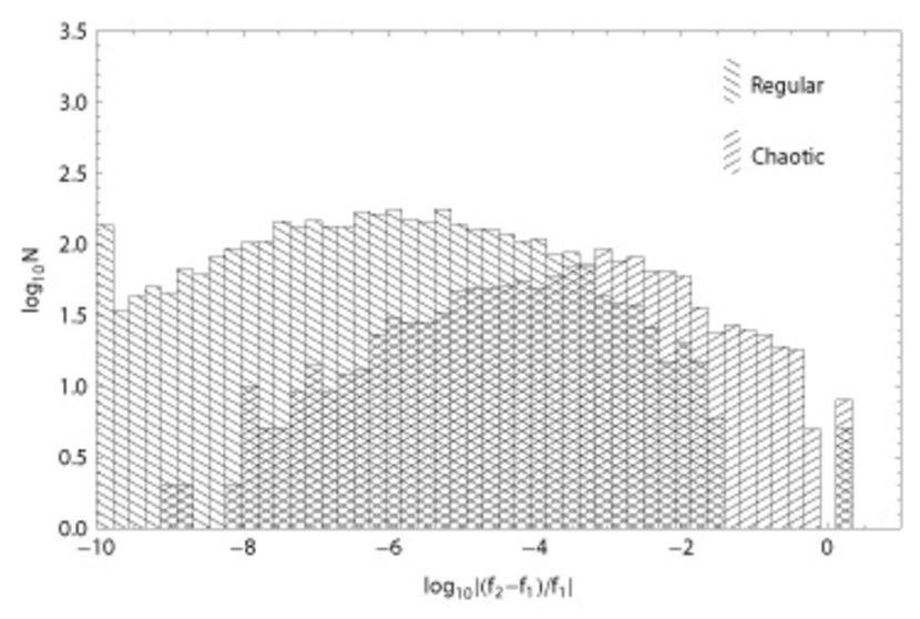
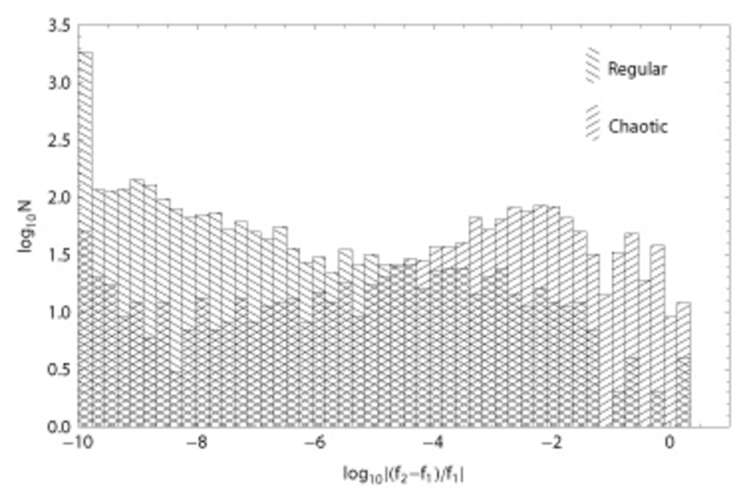
Figure 9: Histograms of frequency differences, separating the regular and chaotic orbits according to the FT-LCNs, using 300 (above) and 4,800 periods (below). In both diagrams the first left column corresponds to all the frequency differences whose logarithm is smaller than $-9.75$.

Table 1: Geometrical distribution of regular, partially chaotic and fully chaotic orbits of our sample.

Type	$a=\langle x^{2}\rangle^{1/2}$	$b=\langle y^{2}\rangle^{1/2}$	$c=\langle z^{2}\rangle^{1/2}$	$b/a$	$c/a$
Regular	$47.96\pm 0.94$	$44.92\pm 0.85$	$45.09\pm 0.86$	$0.936\pm 0.025$	$0.940\pm 0.026$
Part. chaotic	$4.40\pm 0.16$	$3.58\pm 0.17$	$3.72\pm 0.19$	$0.814\pm 0.048$	$0.847\pm 0.053$
Fully chaotic	$2.24\pm 0.04$	$1.92\pm 0.07$	$2.02\pm 0.07$	$0.858\pm 0.034$	$0.904\pm 0.035$

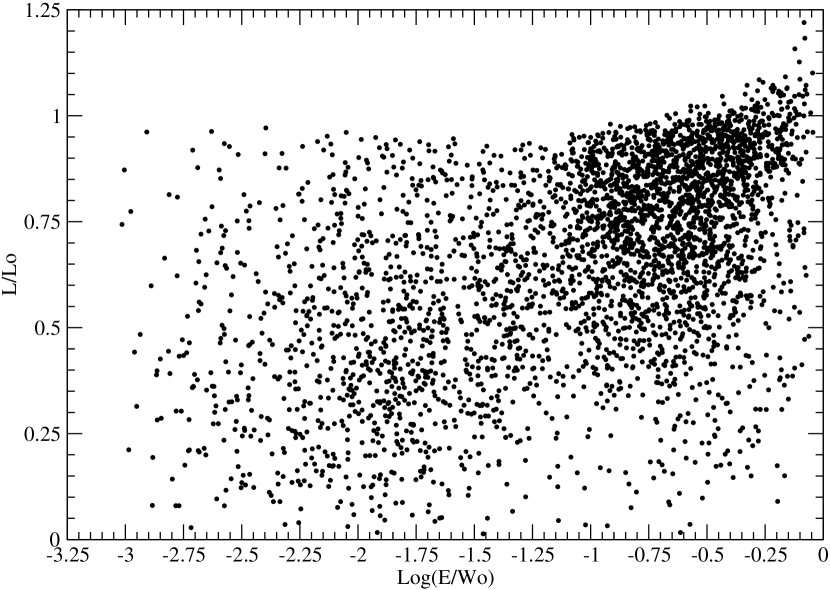
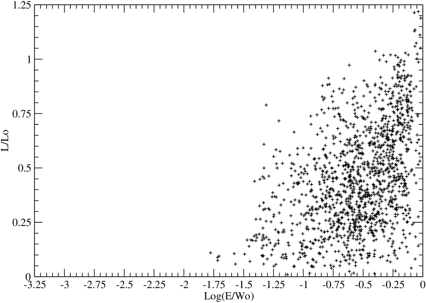
Figure 10: Reduced energy versus reduced initial angular momentum for the regular (above) and chaotic (below) orbits of the sample of 5,000 orbits.

3 Isotropized models

We have now established that there is a significant fraction of chaotic orbits in a model similar to the one of Holley-Bockelmann et al. (2001) and that the reason why they did not find them is, in all likelihood, their use of frequency differences as chaos detector. Nevertheless, the chaotic fraction found in our model is much lower than the fractions typically found in models built from cold collapses and, as indicated in the Introduction, it is possible that the strongly radial orbits resulting from those collapses are the key to explain that difference. Besides, as we have shown, the model we built following the recipe of Holley-Bockelmann et al. (2001) had not reached equilibrium, so that the question remains whether it is possible to build cuspy triaxial models whose velocity distributions are not radially biased, that include significant fractions of chaotic orbits and are highly stable. Therefore, we decided to try to render more isotropic the velocity distribution of a model obtained from a cold collapse and to see whether its chaotic fraction decreases as a result and the final model is stable. Since the models from the first paper of this series (Zorzi & Muzzio, 2012) are, to our knowledge, the ones with the highest fractions of chaotic orbits reported, with less than 25 per cent of regular orbits, they seem to offer a good starting point.

We found that isotropization tends to flatten somewhat the central cusp (see below), so that we chose the model with the steepest central cusp ($\gamma=1.073\pm 0.022$) dubbed E4c which, with only 12.67 per cent regular orbits, is also one of those with highest chaotic content. This model has semiaxes ratios $b/a=0.765$ and $c/a=0.575$, ($a>b>c$ are the square roots of the mean square values of the $x,y,z$ coordinates, respectively, of the 80 per cent most tightly bound particles) and triaxiality $T=(a^{2}-b^{2})/(a^{2}-c^{2})=0.62$. The overall crossing time for this model is $T_{\rm cr}=0.521$ t.u. Fig. 11 (upper left) shows the velocity dispersions in the radial and tangential directions, as well as the velocity anisotropy parameter $\beta$ for this model. A comparison with Fig. 1 (lower right) should take into account the different scales, so that longitudes and velocities from that figure should be multiplied by 0.097 and 2.6, respectively, to switch them to the scales of Fig. 11. With that caveat, it is obvious from the figures that the $\beta$ values from model E4c are substantially higher than those of the model of Section 2 for all ellipsoidal radii.

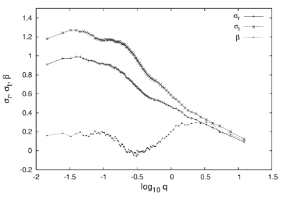
Figure 11: Radial and tangential velocity dispersions, and velocity anisotropy parameter $\beta$, for models: E4c of Paper I (upper left); E4ci (upper right); E4cf6 (lower left); E4cf8 (lower right).

3.1 Isotropization technique

We began selecting at random 25 per cent of the particles from model E4c and, for each particle, we computed the angle $\theta$ between the velocity vector and the radial direction. If $0^{\circ}\leq\theta\leq 60^{\circ}$, then the vector was rotated on the plane defined by the radius and the velocity towards the tangential direction, until it lay in the region $60^{\circ}\leq\theta\leq 90^{\circ}$ (Fig. 12). The actual angle of rotation was computed by linearly mapping the interval $[0^{\circ},60^{\circ}]$ into the interval $[60^{\circ},90^{\circ}]$. The same was done if the velocity vector originally lay in the interval $[120^{\circ},180^{\circ}]$, in which case it was rotated into the region $[90^{\circ},120^{\circ}]$. Alternatively, when the velocity vector made an angle between $60^{\circ}$ and $90^{\circ}$ with the radial direction, it was rotated towards this last direction by mapping linearly from $[60^{\circ},90^{\circ}]$ to $[0^{\circ},60^{\circ}]$. Finally, those velocity vectors lying on $[90^{\circ},120^{\circ}]$ were similarly rotated into the region $[120^{\circ},180^{\circ}]$. Since the $[0^{\circ},60^{\circ}]$ cap around the radial direction has the same area as the $[60^{\circ},90^{\circ}]$ zone, then approximately the same number of velocity vectors were rotated towards the radial direction than towards the tangential direction, thus avoiding any hollowing out of the velocity ellipsoid. But, since the models are originally radially anisotropic, those velocities near the radial direction have bigger moduli than those near the tangential plane and, thus, our procedure extracts ”velocity power” from the radial direction and puts it nearer the tangential plane, i.e., the velocity ellipsoids are left more isotropic than before.

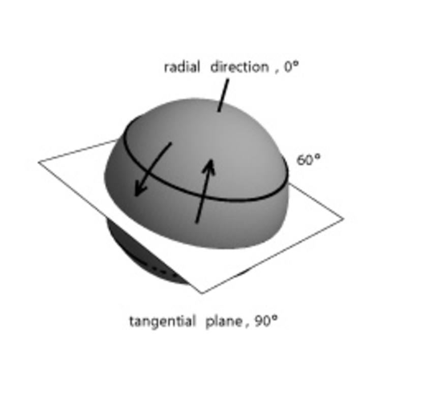
Figure 12: Rotation of the velocity vectors. The spherical surface represents the locus of the unit velocity vectors. The velocities which lie on the radial cap rotate towards the tangential plane, and vice versa.

Once the above procedure was finished, we let the system relax for 10 t.u., which for this model corresponds to about $20T_{\rm cr}$, to allow it to reach a new equilibrium. For this evolution we used the code of Hernquist & Ostriker (1992) with $n=6$ radial terms and $l=4$ angular terms (Zorzi & Muzzio, 2012). After the relaxation, we took another random 25 per cent of particles (from those that had not been chosen before) and repeated the velocity rotation algorithm, followed by another 10 t.u. relaxation period. The rotation plus relaxation process was repeated two more times, thus rotating the velocities of all the particles of the system in the end. The resulting system was allowed to relax an additional $100T_{\rm cr}$ to obtain the final model, dubbed E4ci. It has a fairly isotropic velocity distribution with $\beta\simeq 0$, except at large radii where $\beta>0.2$ (see Fig. 11, upper right). Nevertheless, the central cusp flattened somewhat during the isotropization process, and the final model has $\gamma=0.899\pm 0.019$, still a reasonably steep cusp. We checked the stability of the system by letting it evolve another $400T_{\rm cr}$ and verifying that its global parameters (central density and moments of inertia of the 80 per cent most tightly bound particles) were conserved, just as we had done for the models of Zorzi & Muzzio (2012). The results were even better than those found there, with all the changes smaller than 1 per cent in 100 t.u., i.e., about a Hubble time. In addition to finding those changes from the self–consistent evolution of their models, Zorzi & Muzzio (2012) performed two additional tests for one of them: 1) They fixed the potential before letting the model to evolve (i.e., they eliminated self–consistency); 2) They took one tenth of the particles, and increased ten times their masses, and they let the model evolve self-consistently. The results were that with the fixed potential the evolution was much smaller, and with the reduced number of particles much larger, than for the original model, so that they concluded that most of the evolution was simply due to numerical relaxation in the Hernquist and Ostriker code. Similar tests were done by Aquilano et al. (2007) and (Muzzio et al.2009) using the Aguilar code and they obtained similar results and reached the same conclusion. Thus, the small percentual changes found here are also most likely due to relaxation effects of the $N$–body code and the stability of the model is even better than those percentages indicate. Here we also checked the change in the slope of the central cusp and it turned out to be negligibly small, a mere $-0.03\pm 0.99$ per cent in a Hubble time.

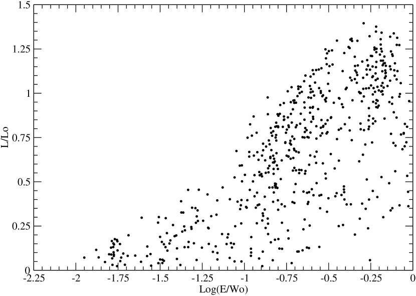
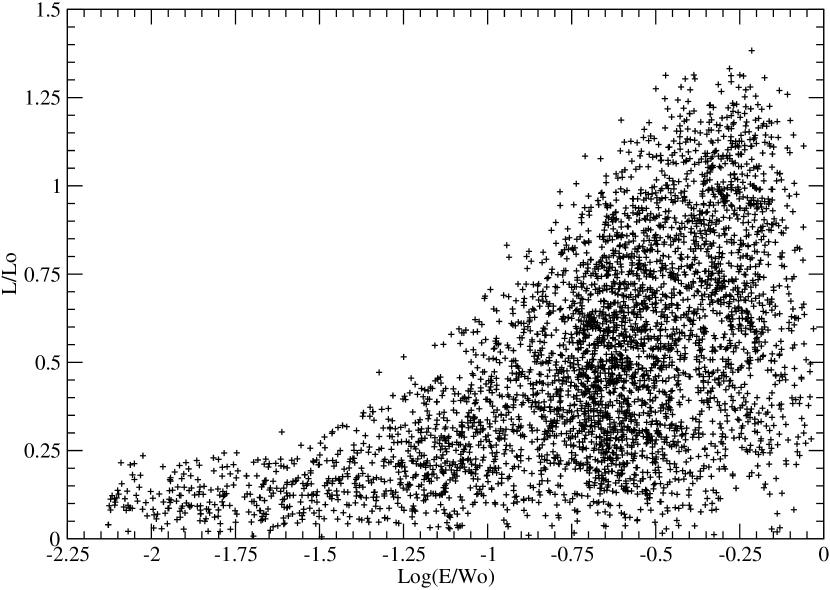
Figure 13: Reduced energy versus reduced initial angular momentum for the original E4c model. The upper and lower panels correspond, respectively, to regular and chaotic orbits.

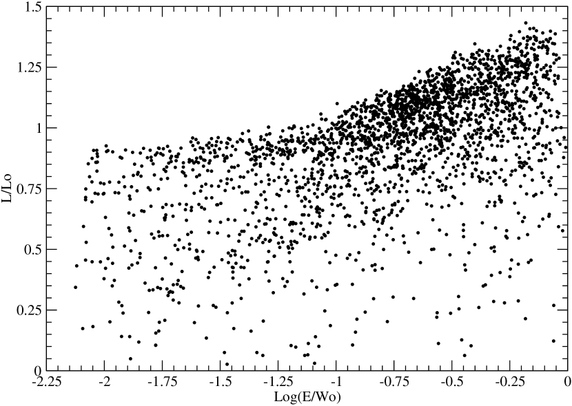
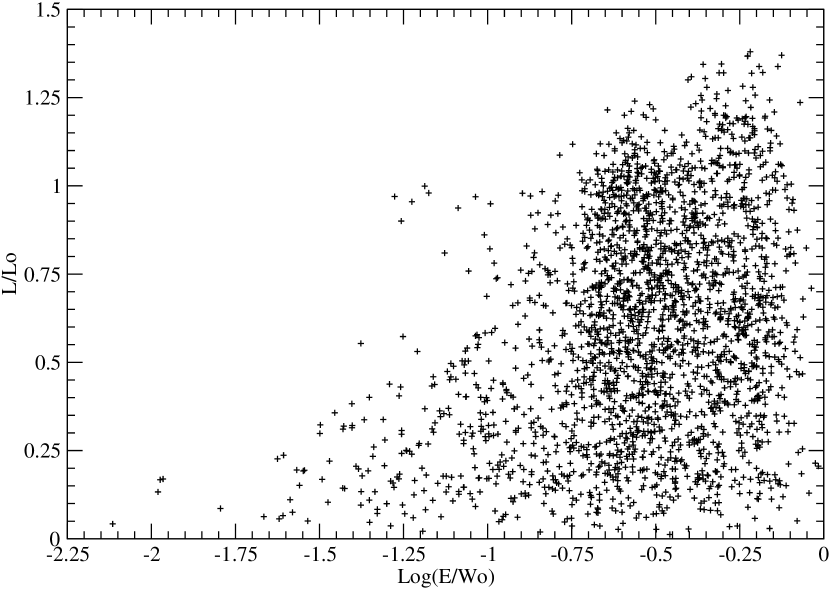
Figure 14: Reduced energy versus reduced initial angular momentum for the isotropized E4ci model. The upper and lower panels correspond, respectively, to regular and chaotic orbits.

Figs. 13 and 14 present the reduced energy versus reduced initial angular momentum, respectively, for the original, E4c, and the isotropized, E4ci, models. It is quite clear the brutal cutoff to the larger angular momenta imposed by the cold collapse used to create model E4c, and how it was compensated by our isotropization technique in model E4ci. Regular and chaotic orbits (see below) are shown separately in both Figures, and it is clear again that chaos is favored by low angular momenta.

The price paid for the isotropization, in addition to the lower cusp slope, was a rounder inertia tensor (see Table 2). In order to try to recover the original triaxiality, we followed the dragging recipe of Holley-Bockelmann et al. (2001), but we applied the squeezing in the $y$ (intermediate) direction only and we modified the time parameters we had used in Section 2 to account for the different values of $T_{\rm cr}$ in the two models. We tried several values of $\xi_{0}$ between 0.5 and 0.8 and finally chose the models we had obtained with $\xi_{0}=0.60$ and $\xi_{0}=0.80$, because they turned out to be the ones more similar to models from Zorzi & Muzzio (2012). After the squeezing had ended, we let the systems relax for $100T_{\rm cr}$ to obtain the final models, which we call E4cf6 (the one obtained with $\xi_{0}=0.60$) and E4cf8 (corresponding to $\xi_{0}=0.80$). We also evolved each one of these two models an additional $400T_{\rm cr}$ interval in order to check their stability and, again, all the changes of the macroscopic parameters and $\gamma$ over a Hubble time were found to be of the order of one per cent.

Table 2 gives the axial ratios of the 20, 40, …, 100 per cent most tightly bound particles for the models. Following Aguilar & Merritt (1990), the axial ratios of the 80 per cent most tightly bound particles are the ones we use to characterize the models, and we see that those ratios are very similar for the present model E4cf6 and the E3 models of Zorzi & Muzzio (2012); also those ratios of our present model E4cf8 are not too different from those of the E4 model of our previous paper. Unfortunately, for other fractions of most tightly bound orbits the differences are larger and the present models tend to be less flattened and less triaxial than those of the first paper in this series. On the other hand, the anisotropy parameter $\beta$ shifted to values somewhat larger than those of model E4ci, although they remain below 0.25 for most radii, and reach about 0.5 only in the outermost regions (Fig. 11). Thus, although the squeezing process raised the anisotropy, we still ended with much more isotropic models than the original E4c. The central cusp maintained a reasonably steep slope in both cases ($\gamma=0.924\pm 0.024$ for the E4cf6 model and $\gamma=0.928\pm 0.024$ for the E4cf8 model).

Table 2: Ratios of semiaxes corresponding to different percentages of most tightly bound particles for our isotropized model and for that model after the squeezing processes. The results for the E3b and E4c models of Zorzi & Muzzio (2012) are also included for comparison.

Model	ratio	20	40	60	80	100
		per cent	per cent	per cent	per cent	per cent
E4ci	$b/a$	0.880	0.889	0.900	0.903	0.869
	$c/a$	0.705	0.685	0.693	0.715	0.800
E4cf8	$b/a$	0.789	0.793	0.804	0.822	0.871
	$c/a$	0.668	0.663	0.655	0.615	0.790
E4cf6	$b/a$	0.760	0.770	0.780	0.797	0.871
	$c/a$	0.712	0.714	0.714	0.683	0.786
E3b	$b/a$	0.710	0.701	0.761	0.802	0.840
	$c/a$	0.554	0.555	0.634	0.692	0.803
E4c	$b/a$	0.749	0.706	0.737	0.765	0.797
	$c/a$	0.588	0.515	0.539	0.575	0.708

3.2 Chaotic content

Just as we had done for the model of Section 2, we used the LIAMAG routine (Udry & Pfenniger, 1988) to obtain the FT-LCNs of 5,000 orbits of each one of the isotropized models; due to the different time scales, the integration time was now 10,000 t.u. and the renormalization interval 1 t.u. Table 3 shows the results, together with those for models E3b and E4c Zorzi & Muzzio (2012) for comparison, and the last column gives the triaxiality, $T=(a^{2}-b^{2})/(a^{2}-c^{2})$, evaluated from the 80 per cent most tightly bound particles. Clearly, the percentages of regular orbits in our isotropized models are much larger than those in the original collapse models, with model E4ci having four or five times more regular orbits than the collapse models of highest chaoticity. Unfortunately the structure of the present models differs from the previous ones, so that we cannot be sure that the difference is due to the different degrees of anisotropy, even though it seems likely.

Reduced energy versus reduced initial angular momenta plots, separating the regular and chaotic orbits, were also done for the E4cf8 and E4cf6 models but, as they turned out to be similar to the one for the E4ci model, of Fig. 14, they are not shown.

Table 3: Percentages of regular, partially chaotic and fully chaotic orbits in the isotropized models. The results for the E3b and E4c models of Zorzi & Muzzio (2012), and the triaxiality of each model, $T$, are also included for comparison.

Model	Regular	Part. Chaotic	Fully Chaotic	$T$
	(per cent)	(per cent)	(per cent)
E4ci	$50.16\pm 0.71$	$9.18\pm 0.41$	$40.66\pm 0.69$	0.38
E4cf8	$41.28\pm 0.70$	$9.24\pm 0.41$	$49.48\pm 0.71$	0.52
E4cf6	$45.88\pm 0.70$	$11.04\pm 0.44$	$43.08\pm 0.70$	0.68
E3b	$14.04\pm 0.50$	$13.57\pm 0.49$	$72.39\pm 0.64$	0.68
E4c	$12.67\pm 0.49$	$10.11\pm 0.45$	$77.22\pm 0.62$	0.62

Table 4: Orbital classification of the regular orbits in the isotropized models. The results for the E3b and E4c models of Muzzio et al. (2013) are also included for comparison.

Model	BBL	SAT	ILAT	OLAT
	(per cent)	(per cent)	(per cent)	(per cent)
E4ci	1.72 $\pm$ 0.26	81.53 $\pm$ 0.78	0.16 $\pm$ 0.08	16.59 $\pm$ 0.74
E4cf8	4.43 $\pm$ 0.45	73.98 $\pm$ 0.97	1.07 $\pm$ 0.23	20.52 $\pm$ 0.89
E4cf6	3.23 $\pm$ 0.37	59.02 $\pm$ 1.03	4.40 $\pm$ 0.43	33.35 $\pm$ 0.98
E3b	23.00 $\pm$ 1.61	53.86 $\pm$ 1.90	6.84 $\pm$ 0.96	13.10 $\pm$ 1.29
E4c	26.78 $\pm$ 1.85	66.43 $\pm$ 1.97	4.00 $\pm$ 0.82	0.70 $\pm$ 0.35

4 Regular orbits

As in our previous papers (Aquilano et al., 2007; Muzzio, Navone & Zorzi, Muzzio et al.2009; Muzzio, Navone & Zorzi, 2013), we used frequency analysis to classify the regular orbits and the results are presented in Table 4 together with those for our E3b and E4c previous models, for comparison. There are clear decreases in the percentages of boxes and boxlets (BBLs) and clear increases in the percentages of outer long axis tubes (OLATs) as we go from the original to the isotropized models. The fraction of small axis tubes (SATs) seems to be larger for the E4ci and E4cf8 models, but these models have smaller triaxility than models E3b and E4c (see Table 3); model E4cf6, whose triaxiality is equal to that of model E3b, and not too different from that of model E4c, has a fraction of SATs similar to the original models. The percentages of inner long axis tubes (ILATs) seem to be smaller in the isotropized models, but these fractions are generally low anyway.

5 Conclusions

We have used the adiabatic dragging of Holley-Bockelmann et al. (2001) to build up a cuspy triaxial model similar to the one they had investigated. Using a longer relaxation time than the one they had used we found that the model had not reached equilibrium at the latter time. The cusp, in particular, steadily reduces its slope and, after $100T_{\rm cr}$, it is only $\gamma\simeq 0.8$. Nevertheless, we searched for chaotic orbits in that model as Holley-Bockelmann et al. (2001) had done and we found that, on the one hand, the frequency difference technique they had used is not adequate and is the likely culprit of their finding almost no chaos and, on the other hand, that when other techniques (such as Lyapunov exponents and SALI) are used, it turns out that more than one fourth of the orbits are chaotic. Moreover, chaoticity affects the distribution of orbits, so that it should be taken into account in the study of the structure of the model. The model of Holley-Bockelmann et al. (2001) was the only cuspy and triaxial system built with the $N$–body method where almost no chaos had been found, so that our result solves that puzzle.

Nevertheless, the chaotic fraction we found is still substantially lower than that of other models built with the $N$–body method (, Muzzio et al.2009; Zorzi & Muzzio, 2012), so that we investigated whether the extreme velocity anisotropy of the latter could explain that difference. We succeeded in rendering the velocity distribution of one of the models of Zorzi & Muzzio (2012) much less radially oriented and, thus, more isotropic and we also applied the adiabatic drag to the isotropized model to obtain two other more triaxial systems. The chaotic fractions in these models are in the 50 to 60 percent range, substantially lower than the 75 to 90 per cent range found in the models of Zorzi & Muzzio (2012). Unfortunately, although the semiaxial ratios of the 80 per cent most tightly bound particles of the isotropized models are similar to those of some of the original models, those ratios differ for other fractions of most tightly bound particles, so that the models are not strictly comparable. Nevertheless, the fact that $\it all$ the isotropized models have lower chaoticity than $\it any$ of the original collapse models strongly suggests that the radially oriented orbits of the latter favored the onset of chaoticity.

Finally, our results clearly show that one can obtain cuspy triaxial models with fairly isotropic velocity distributions that contain large fractions of chaotic orbtis and, nevertheless, are highly stable so that, in this sense, they extend our similar previous results for models with strongly radial velocity distributions.

References

- Aguilar & Merritt (1990) Aguilar L.A., Merritt D., 1990, ApJ, 354, 33
- Aquilano et al. (2007) Aquilano R.O., Muzzio J.C., Navone H.D., Zorzi A.F., 2007, Cel. Mech. Dyn. Astr., 99, 307
- Dubinski & Carlberg (1991) Dubinski J., Carlberg R., 1991, ApJ, 378, 496
- Hernquist (1990) Hernquist L., 1990, ApJ, 356, 359
- Hernquist & Ostriker (1992) Hernquist L., Ostriker J.P., 1990, ApJ, 386, 375