A Low-Complexity Detector for Memoryless Polarization-Multiplexed Fiber-Optical Channels

Abstract

A low-complexity detector is introduced for polarization-multiplexed $M$-ary phase shift keying modulation in a fiber-optical channel impaired by nonlinear phase noise, generalizing a previous result by Lau and Kahn for single-polarization signals. The proposed detector uses phase compensation based on both received signal amplitudes in conjunction with simple straight-line rather than four-dimensional maximum-likelihood decision boundaries.

I Introduction

The Manakov equation describes the propagation of a polarization-multiplexed signal in a fiber-optical channel. Two major impairments, linear chromatic dispersion and the Kerr nonlinear effect, are modeled by this equation. The nonlinear effect causes a phase rotation proportional to the field instantaneous power. The interaction of the signal and the amplified spontaneous emission (ASE) noise generated by optical amplifiers due to the nonlinear Kerr effect gives rise to nonlinear phase noise (NLPN). NLPN imposes a major degradation in the performance of coherent optical data transmission systems.

Bononi et al. [1] investigated the effect of NLPN on popular modulation formats for single-channel and wavelength-division multiplexing systems in a dispersion-managed fiber link. The performance of orthogonal frequency-division multiplexing systems in the presence of NLPN has been evaluated in [2] by theoretical, numerical, and experimental approaches. In [3],[4, ch. 4], comprehensive surveys of known techniques for the analysis and characterization of NLPN and its impact on the system performance are provided.

The statistics of NLPN and the detector design for a channel with NLPN have been studied in [5, 6, 7] by analytical approaches and in [8] by numerical methods. The joint probability density function (pdf) of the received amplitude and phase given the initial amplitude and phase of the transmitted signal and the optical signal-to-noise ratio (OSNR) is derived in [9, 5, 10] [4, pp. 157, 224–225] for a fiber-optical channel with NLPN caused by distributed or lumped amplification. Moreover, compensation of NLPN has been studied in [11] based on the aforementioned pdf.

In this paper, we extend the detector structure introduced for a single polarization (SP) $M$-PSK system in [11] to polarization-multiplexed (PM) $M$-PSK, using the signal statistics derived in [12]. To this end, we first introduce a simplified approach to reproduce the result in [11] for the SP case. This method can be easily used to extend the result to the PM case and can also be applied to both lumped and distributed amplification. For simplicity, we assume single-channel transmission and inter-channel effects are not taken into consideration. The symbol error rate (SER) of the proposed detector is compared to the performance of the maximum-likelihood (ML) detector for PM-$4$-PSK and to the performance of the ML detector for SP-$4$-PSK for the same bandwidth as well as for the same data rate.

II System Model and Preliminaries

We assume zero dispersion to make the analysis applicable to memoryless (nondispersive) fiber-optical channels, similarly as in, e.g., [13, 5, 8, 10, 11]. Due to this assumption, the subsequent analysis ignores the interaction of chromatic dispersion and nonlinearity. The resulting model can serve as an approximation for dispersion-managed transmission links provided that the local accumulated dispersion is sufficiently low [1, 12]. For a zero polarization-mode and chromatic dispersion fiber-optical channel, the Manakov equation with loss included reduces to [14, ch. 6]

$$j{\partial\mathbf{E}\over\partial z}+\gamma(\mathbf{E}\mathbf{E}^{{\dagger}})\mathbf{E}+j{\alpha\over 2}\mathbf{E}=\mathbf{0},$$ (1)

where $\mathbf{E}=(E_{\text{x}},E_{\text{y}})$ is the polarization-multiplexed launched envelope signal into the fiber, $\gamma$ is the nonlinear coefficient, $\alpha$ is the attenuation coefficient, ${\dagger}$ denotes Hermitian conjugation, and $z$ is the distance from the beginning of the fiber. The solution to (1) at time $t$ can be written as [14, ch. 4]

$$\mathbf{E}(z,t)=\mathbf{E}(0,t)q(z)\exp\left(j\gamma P_{0}(t)\int_{0}^{z}q^{2}(\tau)\,\text{d}\tau\right),$$ (2)

where $P_{0}(t)=|E_{\text{x}}(0,t)|^{2}+|E_{\text{y}}(0,t)|^{2}$ is the instantaneous launched power into the fiber and $q(z)=\exp(-\alpha z/2)$ is a function that describes the power evolution.

Here, we assume a fiber link with total length $L$ and either distributed or lumped amplification to compensate for the fiber loss perfectly. We consider ASE noise within the optical signal bandwidth, i.e., ignoring the Kerr effect induced from out-of-band signal and noise in the same way as in [13]. If a four-dimensional (4D) signal $\mathbf{S}=(S_{\text{x}},S_{\text{y}})$, consisting of two two-dimensional (2D) complex signals, is transmitted, it experiences an overall NLPN $\phi_{\text{NL}}=\phi_{\text{x}}+\phi_{\text{y}}$. The terms $\phi_{\text{x}}$ and $\phi_{\text{y}}$ are generated by the interaction of the signal and noise due to the Kerr effect in polarizations x and y, respectively. For lumped amplification and a link consisting of $N$ spans, ASE noise $n_{\text{x}}^{i}$, $i=1,\ldots,N$, with variance $\sigma_{0}^{2}$ is added after each span. One may use (2) to obtain $\phi_{\text{x}}=\gamma L_{\text{eff}}\sum_{i=1}^{N}|S_{\text{x}}+\sum_{l=1}^{i}n_{\text{x}}^{l}|^{2}$, where $L_{\text{eff}}=(1-\exp(-\alpha L/N))/\alpha$ is the effective nonlinear length. It is clearly seen that signals in both polarizations contribute to the generated NLPN $\phi_{\text{NL}}$. The received electric field $\mathbf{E}$ can be written as $\mathbf{E}=\hat{\mathbf{E}}e^{-j\phi_{\text{NL}}}$, where $\hat{\mathbf{E}}=\mathbf{S}+\sum_{i=1}^{N}\mathbf{n}^{i}$ is the linear part of the electric field and $\mathbf{n}^{i}=(n_{\text{x}}^{i},n_{\text{y}}^{i})$. One may regard distributed amplification as lumped amplification with an infinite number of spans. This gives $\lim_{N\rightarrow\infty}NL_{\text{eff}}=L$. In this case, a continuous amplifier noise vector $\mathbf{n}(z)=(n_{\text{x}}(z),n_{\text{y}}(z))$ is considered. The elements of this vector are zero-mean complex-valued Wiener processes [4, p. 154] with autocorrelation function $\text{E}[n_{\text{x}}(z_{1})n_{\text{x}}^{*}(z_{2})]\!\!=\sigma_{\text{d}}^{2}\text{min}(z_{1},z_{2}),$ where $\sigma_{\text{d}}^{2}=2h\nu_{\text{opt}}W\alpha n_{\text{sp}}$ [11], $h\nu_{\text{opt}}$ is the energy of a photon, $n_{\text{sp}}$ is the spontaneous emission factor, and $W$ is the bandwidth of the optical signal. The SNR vector is defined as $\boldsymbol{\rho}=(\rho_{\text{x}},\rho_{\text{y}})$ where $\rho_{\text{x}}$ is $|S_{\text{x}}|^{2}/(L\sigma_{\text{d}}^{2})$ or $|S_{\text{x}}|^{2}/(N\sigma_{0}^{2})$ for distributed or lumped amplification, respectively. The normalized received amplitude $r_{\text{x}}$ is denoted by $|E_{\text{x}}|/(\sigma_{\text{d}}\sqrt{L})$ or by $|E_{\text{x}}|/(\sigma_{0}\sqrt{N})$ for distributed and lumped amplifications.

The joint pdf of the received phase vector $\boldsymbol{\theta}=(\theta_{\text{x}},\theta_{\text{y}})$ and the normalized amplitudes $\mathbf{r}=(r_{\text{x}},r_{\text{y}})$ of a zero-dispersion fiber-optical channel is [12]

$$f_{\boldsymbol{\Theta},\mathbf{R}}(\boldsymbol{\theta},\mathbf{r})={f_{\mathbf{R}}(\mathbf{r})\over 4\pi^{2}}+{1\over 2\pi^{2}}\sum\limits_{k_{\text{x}}=1}^{\infty}\text{Re}\left\{C_{\mathbf{k}_{\text{x}}}(\mathbf{r})e^{jk_{\text{x}}\theta_{\text{x}}}\right\}$$

$$\qquad+{1\over 2\pi^{2}}\sum\limits_{k_{\text{x}}=1}^{\infty}\sum\limits_{k_{\text{y}}=1}^{\infty}\text{Re}\left\{C_{\mathbf{k}}(\mathbf{r})e^{j\mathbf{k}\cdot\boldsymbol{\theta}}+C_{\mathbf{k^{*}}}(\mathbf{r})e^{j\mathbf{k^{*}}\cdot\boldsymbol{\theta}}\right\}$$

$$\qquad\qquad\qquad+{1\over 2\pi^{2}}\sum\limits_{k_{\text{y}}=1}^{\infty}\text{Re}\left\{C_{\mathbf{k}_{\text{y}}}(\mathbf{r})e^{jk_{\text{y}}\theta_{\text{y}}}\right\},$$ (3)

where $f_{\mathbf{R}}(\mathbf{r})$ is the joint pdf of the two normalized independent Ricean random variables $r_{\text{x}}$ and $r_{\text{y}}$, and the Fourier coefficients $C_{\mathbf{k}}(\mathbf{r})$ are given in [12]. In (II), we assume the transmitted phase vector to be $(0,0)$. Due to the rotational invariance of the channel, the pdf for an arbitrary transmitted phase vector $(\theta_{0,\text{x}},\theta_{0,\text{y}})$ is obtained by replacing $\theta_{\text{x}}$ and $\theta_{\text{y}}$ in (II) with $\theta_{\text{x}}-\theta_{0,\text{x}}$ and $\theta_{\text{y}}-\theta_{0,\text{y}}$, respectively.

For an SP scheme, the joint pdf of the phase and the normalized amplitude of the received signal in the corresponding polarization is simplified to [4, ch. 5]

$$f_{\Theta,R}(\theta,r)\!=\!{f_{R}(r)\over 2\pi}\!+\!{1\over\pi}\sum\limits_{k=1}^{\infty}\text{Re}\left\{C_{k}(r)e^{jk\theta}\right\},$$ (4)

where $f_{R}(r)$ is the Ricean pdf of the amplitude $r$, and the Fourier coefficients $C_{k}(r)$ are given in [12] for both types of amplifications. Again, the transmitted phase in (4) is assumed to be 0, and the pdf for an arbitrary transmitted phase $\theta_{0}$ is obtained by replacing $\theta$ with $\theta-\theta_{0}$.

In the following, we consider $M$-PSK constellations with $s_{k}=\sqrt{E_{\text{s}}}\exp\left(j{\pi\over M}(2k+1)\right)$, $k=0,\ldots,M-1$, where $E_{\text{s}}$ is the average energy of the constellation.

III The ML Receiver for SP-$M$-PSK

For SP-$M$-PSK, the optimal decision (Voronoi) regions for the received constellation have spiral shape (cf. [11, Fig. 1]), and hence ML detection is computationally complex. To decrease the complexity of the detector, Lau and Kahn showed that straight-line decision boundaries can be used, provided that an amplitude-dependent phase rotation $\theta^{c}$ is applied before detection [11]. The corresponding receiver structure is illustrated in the top half of Fig. 1(a). It can be seen that the phase rotation is solely a function of the received amplitude in one polarization and a simple ML detection of $M$-PSK for additive white Gaussian noise (AWGN) with straight-line decision boundaries is subsequently performed.

(a)

(b)

Figure 1: Receiver for PM-$M$-PSK with (a) separate detection (PM-Det1) and (b) joint calculation of the amplitude-dependent phase rotations (PM-Det2).

In this section, we introduce a new approach to derive the optimal phase rotation as a function of the received amplitude. In contrast to [11], this approach can be easily extended to PM-$M$-PSK. For a transmitted phase of $\theta_{0}=0$, we assume that the conditional pdf $f_{\Theta|R}(\theta|r)$ of the received phase $\theta$ given the received amplitude $r$ is approximately symmetric around $\theta_{\text{max}}(r)$, where $\theta_{\text{max}}(r)$ denotes the phase value where $f_{\Theta|R}(\theta|r)$ is maximum. This assumption is motivated by inspection of the pdf and its validity is justified later by the obtained results. In fact, an equivalent approximation was also done in [11, App. A]. This assumption is used for both distributed and lumped amplifications.

Lemma 1

Let $f_{X}(x)$ be the (periodic) pdf of a random angle $X$. Furthermore, let the pdf be symmetric around $x_{\text{max}}\in(-\pi,\pi]$, the value where $f_{X}(x)$ has its maximum. If the pdf decreases monotonically from $x_{\text{max}}$ to $x_{\text{max}}\pm\pi$, then $x_{\text{max}}=-\arg\Psi_{X}(1)$, where $\Psi_{X}(\nu)$ is the (discrete) characteristic function (CF) of $X$.

Proof:

Define $\tilde{X}=X-x_{\text{max}}$. Since the pdf of $\tilde{X}$ is an even function, its CF is real. Furthermore, the CFs of $X$ and $\tilde{X}$ are related via $\Psi_{X}(\nu)=\Psi_{\tilde{X}}(\nu)e^{-j\nu x_{\text{max}}}$. Letting $\nu=1$ and solving for $x_{\text{max}}$ gives $x_{\text{max}}=\arg\Psi_{\tilde{X}}(1)-\arg\Psi_{X}(1)$. Thus, it needs to be shown that $\arg\Psi_{\tilde{X}}(1)=0$. Having already established that $\Psi_{\tilde{X}}(1)$ is real, we only need to show that it is also positive. This follows from the definition $\Psi_{\tilde{X}}(1)=\int_{-\pi}^{\pi}f_{\tilde{X}}(x)\cos(x)\,\text{d}x$ and the fact that $f_{\tilde{X}}(x)$ is nonnegative and decreases monotonically from $0$ to $\pm\pi$. ∎

Using Lemma 1, one can compute the rotation of the $M$-PSK ML decision boundaries due to NLPN as described in the following theorem.

Theorem 1

Consider a memoryless fiber-optical channel with NLPN. The decision boundary of the ML detector for SP-$M$-PSK between symbols $s_{k}$ and $s_{k+1}$ has the polar coordinates $(r,\theta_{b}(k,r))$, where $\theta_{b}(k,r)=-C_{1}(r)+2k/M$ for $r\geq 0$ and $C_{1}$ is the first Fourier coefficient in (4).

Proof:

The ML decision boundary between the two symbols of the $M$-PSK constellation with $k=0$ and $k=M-1$ is determined in such a way as to satisfy

$$f_{\Theta|R,\Theta_{0}}(\theta^{\text{c}}(r)\mid r,-\tfrac{\pi}{M})=f_{\Theta|R,\Theta_{0}}(\theta^{\text{c}}(r)\mid r,\tfrac{\pi}{M}).$$

Using the symmetry of $f_{\Theta|R,\Theta_{0}}(\theta|r,\theta_{0})$ around $\theta_{\text{max}}(r)+\theta_{0}$, we obtain $\theta^{\text{c}}(r)=\theta_{\text{max}}(r)$. Using Lemma 1, we get $\theta_{\text{max}}(r)=-\arg~{}\Psi_{\Theta|R,\Theta_{0}}(1\mid r,0)=-\arg C_{1}(r)$. ∎

IV Receivers for PM-$M$-PSK

For a fixed state of polarization, we receive two dependent 2D symbols, which have been rotated by the NLPN equally. Using (II), the ML detector in this case can be written as

$${\boldsymbol{\hat{\theta}}}_{0}=\arg\max_{\boldsymbol{\theta}_{0}}f_{\boldsymbol{\Theta},\boldsymbol{R}|\boldsymbol{\Theta}_{0}}(\boldsymbol{\theta},\boldsymbol{r}|\boldsymbol{\theta}_{0}).$$ (5)

The optimization is performed over all possible $M^{2}$ transmitted phase combinations for a PM-$M$-PSK signal. We refer to this detector as “PM-ML”.

A simple, but clearly suboptimal, way to reduce the complexity of solving (5) is to treat the received signals in both polarizations independently. In other words, the marginal pdfs $f_{\Theta_{\text{x}},R_{\text{x}}}(\theta_{\text{x}},r_{\text{x}})$ and $f_{\Theta_{\text{y}},R_{\text{y}}}(\theta_{\text{y}},r_{\text{y}})$ are used to perform detection separately in each polarization, which leads again to spiral-shaped decision boundaries as in Sec. III. Equivalently, one may extend the receiver structure for SP in a straightforward manner as shown in Fig. 1(a), where a different rotation angle is applied to each received symbol, based on the received amplitude in the corresponding polarization. Using Theorem 1, the computation of the rotation angles is then based on the first Fourier coefficient of the two marginal pdfs. We refer to this detector as “PM-Det1”.

As seen in (2), the phase rotation due to the nonlinear Kerr effect is a function of the signal amplitudes in both polarizations. Hence, one may improve the performance of PM-Det1 by taking into account the amplitudes of both polarizations in computing the phase rotation. To this end, we use the same symmetry assumption as in the previous section for $f_{\Theta_{\text{x}}|\mathbf{R}}(\theta|\mathbf{r})=f_{\Theta_{\text{x}},\mathbf{R}}(\theta,\mathbf{r})/f_{\mathbf{R}}(\mathbf{r})$, where $f_{\Theta_{\text{x}},\mathbf{R}}(\theta,\mathbf{r})$ is the marginal of (II) with respect to $\Theta_{\text{y}}$, i.e., we assume that $f_{\Theta_{\text{x}}|\mathbf{R}}(\theta|\mathbf{r})$ is symmetric around the phase for which this pdf is maximum. This assumption allows us to describe the decision boundaries of the PM-$M$-PSK signal distorted by NLPN in each polarization as the rotated version of the straight-line decision boundaries for an AWGN channel.

Theorem 2

The decision boundaries of the detector given by

$$\hat{\theta}_{0,\text{x}}=\arg\max_{{\theta}_{0,\text{x}}}f_{\Theta_{\text{x}},\boldsymbol{R}|{\theta}_{0,\text{x}}}({\theta}_{\text{x}},\boldsymbol{r}|{\theta}_{0,\text{x}})$$ (6)

for polarization x can be transformed to straight lines using the phase rotation given by

$$\theta^{\text{c}}_{\text{x}}(\mathbf{r})=-\arg C_{(1,0)}(\mathbf{r}),$$ (7)

where $C_{(1,0)}(\mathbf{r})$ is the Fourier coefficient appearing in (II) with $\boldsymbol{k}_{x}=(1,0)$. Similarly, the rotation for polarization y is obtained as $\theta^{\text{c}}_{\text{y}}(\mathbf{r})=-\arg C_{(0,1)}(\mathbf{r})$.

Proof:

One may follow an analogous approach as in the proof of Theorem 1, by replacing $f_{\Theta_{\text{x}}|\mathbf{R}}(\theta|\mathbf{r})$ with $f_{\Theta|R}(\theta|r)$ to show that the decision boundary between symbols $S_{x}=s_{k}$ and $S_{x}=s_{k+1}$ in polarization x has the parametric description $r_{\text{x}}\exp(j\theta^{\text{c}}_{\text{x}}(\mathbf{r})+2jk\pi/M)$. ∎

The proposed detector implementing (6) via this phase rotation method is referred to as “PM-Det2” and shown in Fig. 1(b). It can be seen that the rotation angle in each polarization is computed using the received amplitudes $\mathbf{r}$. It is worth mentioning that since the rotation is an invertible operation, joint 4D demodulation is still possible after the rotation. For complexity reasons, however, we perform hard decision on each 2D soft symbol using simple straight-line decision boundaries as shown in the figure.

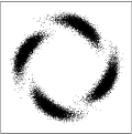
(a) no comp.

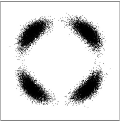
(b) $\theta_{\text{x}}^{c}=f(r_{\text{x}})$

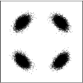
(c) $\theta_{\text{x}}^{c}=f(\boldsymbol{r})$

Figure 2: Scatter plots in the x polarization for (a) no compensation, (b) compensation according to Fig. 1(a), and (c) according to Fig. 1(b). Decision boundaries in (b) and (c) are straight lines. In (a), the boundaries are spiral shaped and depend on the received amplitude in the y polarization.

In Fig. 2, a qualitative comparison of the two different rotation schemes corresponding to PM-Det1 and PM-Det2 is shown. Fig. 2(a) shows a scatter plot of the received symbols in polarization x directly after the channel, i.e., no phase compensation is assumed. In Fig. 2(b), a phase rotation of each received symbol is applied, which is solely based on the corresponding received amplitude of this symbol (PM-Det1). Lastly, Fig. 2(c) shows the result of applying a phase rotation that is based on the received amplitude of the received symbols in both polarizations (PM-Det2). Observe that the second rotation method leads to a notably smaller phase variance compared to the first method. However, it should be mentioned that the receiver structure shown in Fig. 1(b) does not correspond to the ML receiver for PM-$M$-PSK, since the residual phases in both polarizations after the rotation are not statistically independent. The performance loss compared to ML detection is quantified in the next section.

V Performance Analysis

The SER of PM-$M$-PSK for PM-Det1 and PM-Det2 can be computed analytically. After the introduced phase rotations, the marginal pdf of the phase in polarization x, given that the phase of the transmitted signal is zero, is obtained by replacing $\theta_{\text{x}}$ with $\theta^{\prime}_{\text{x}}-\theta^{\text{c}}_{\text{x}}$ in $f_{\Theta_{\text{x}}|\mathbf{R}}(\theta|\mathbf{r})$ and then integrating out the radii $r_{\text{x}}$ and $r_{\text{y}}$ over $[0,+\infty)$ to get

$$f_{\Theta^{\prime}_{\text{x}}}(\theta)={1\over 2\pi}+{1\over\pi}\sum\limits_{k=1}^{\infty}\cos(k\theta)\int\limits_{0}^{\infty}\int\limits_{0}^{\infty}|C_{(k,0)}(\mathbf{r})|\text{d}r_{\text{x}}\text{d}r_{\text{y}}.$$ (8)

Here, we only show how to compute the SER of PM-Det2 for a PM-$M$-PSK system. An analogous derivation can be applied for PM-Det1. One can write

$$\text{SER}_{\text{x}}=1-\int_{-{\pi\over M}}^{{\pi\over M}}f_{\Theta^{\prime}_{\text{x}}}(\theta)\text{d}\theta={M-1\over M}-$$

$$\sum_{k=1}^{\infty}\frac{2\text{sinc}\left({k\over M}\right)}{M}\int_{0}^{\infty}\!\!|C_{(k,0)}^{\text{x}}(r_{\text{x}})|\text{d}r_{\text{x}}\!\int_{0}^{\infty}\!\!|C_{(k,0)}^{\text{y}}(r_{\text{y}})|\text{d}r_{\text{y}},$$

where $C_{(k,0)}^{\text{x}}$ and $C^{\text{y}}_{(k,0)}$ are computed using [12, eq. (26)].

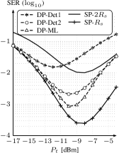
(a) analytical SER with zero dispersion

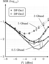
(b) simulated SER for a dispersion-managed link

Figure 3: The SER of SP and PM systems with 4-PSK versus the transmitted power per polarization $P_{\text{t}}$.

In Fig. 3(a), the performance of PM-$4$-PSK is evaluated using the above analytical approach for PM-Det1 and PM-Det2. The SER of the ML detector defined by (6) is given by a four-dimensional integral of the pdf over the ML decision regions. This SER, estimated by Monte-Carlo integration, is also shown in Fig. 3(a). Moreover, we compute the SER of SP-$4$-PSK to compare with SP data transmission in two different scenarios: (i) For the same data rate per polarization (i.e., the same bandwidth) and (ii) for the same total data rate as the PM case. This evaluation is done for distributed amplification with channel parameters $L=9000$ km, $\gamma=1.4~{}\text{W}^{-1}\text{km}^{-1}$, $R_{\text{s}}=28$ Gbaud, $\nu_{\text{opt}}=193.55$ THz, $\alpha=0.25$ dB/km, and $F_{n}=6$ dB. As seen in Fig. 3(a), the PM schemes show negligible performance degradation in the linear regime for a fixed bandwidth (case (i)), i.e., for $P_{\text{t}}<-15$ dBm, compared to the SP scheme. For a fixed data rate (case (ii)), one may observe a $2$ dB performance improvement using PM-Det2, at a SER of $1.5\times 10^{-2}$. In the strongly nonlinear regime, the SP scheme is superior to PM at the expense of losing half of the data rate. Furthermore, in the linear regime, the SP scheme in case (i) and the PM scheme have the same performance and their SER curves overlap, while in the strongly nonlinear regime, the SER of the PM scheme converges to the SER of the SP scheme in case (ii). This is because the system performance is intimately related to the product of the noise variance and the transmit power in the nonlinear regime, which is the same for these two scenarios. Fig. 3(a) also indicates that in the linear regime, the detectors PM-Det2 and PM-Det1 perform similarly. However, the reduction in circular variance observed in Fig. 2 translates into a noticeably better SER in the nonlinear regime for PM-Det2 when compared to PM-Det1. In the region of interest, i.e., SNRs around $-10$ dBm, the performance degradation of PM-Det2 compared to the ML detector is $0.7$ dB. This is due to independent detection of phase information in the two polarizations. In Fig. 3(b), we also show the performance of DP-Det1 and DP-Det2 for a dispersion-managed link using the split step Fourier method. The system parameters are the same as before, but now we assume $45$ fiber spans of length $90$ km and a lumped amplification scheme. Dispersion is compensated after each span using an ideal dispersion-compensating fiber. The symbol rate is varied between $0.5$ and $5$ Gbaud to determine the robustness of the detector with respect to residual dispersion. The memoryless pdf loses its accuracy for high symbol rates due to the strong interaction between nonlinearities and dispersion and therefore the superiority of the proposed detector disappears for these parameters and symbol rates higher than 3 Gbaud. Similar observations regarding the accuracy of the memoryless model have been made in [12].

VI Conclusion

A low-complexity detector is proposed for memoryless polarization-multiplexed fiber-optical channels by compensating the amplitude-dependent NLPN. The compensation is performed by a phase rotation of the received symbols depending on the amplitudes in both polarizations. The performance results confirm the superiority of PM schemes to SP for the same data rate.

References

- [1] A. Bononi, P. Serena, and N. Rossi, “Modeling of signal-noise interactions in nonlinear fiber transmission with different modulation formats,” in Proc. European Conf. Optical Communication (ECOC), Vienna, Austria, 2009.
- [2] X. Yi, W. Shieh, and Y. Ma, “Phase noise effects on high spectral efficiency coherent optical OFDM transmission,” J. Lightw. Technol., vol. 26, no. 10, pp. 1309–1316, May 2008.
- [3] A. Demir, “Nonlinear phase noise in optical-fiber-communication systems,” J. Lightw. Technol., vol. 25, no. 8, pp. 2002–2032, Aug. 2007.
- [4] K.-P. Ho, Phase-Modulated Optical Communication Systems. Springer, 2005.
- [5] A. Mecozzi, “Probability density functions of the nonlinear phase noise,” Opt. Lett., vol. 29, no. 7, pp. 673–675, 2004.
- [6] S. Kumar, “Analysis of nonlinear phase noise in coherent fiber-optic systems based on phase shift keying,” J. Lightw. Technol., vol. 27, no. 21, pp. 4722–4733, Nov. 2009.
- [7] Y. Yadin, M. Shtaif, and M. Orenstein, “Nonlinear phase noise in phase-modulated WDM fiber-optic communications,” IEEE Photon. Technol. Lett., vol. 16, no. 5, pp. 1307–1309, May 2004.
- [8] C. Häger, A. Graell i Amat, A. Alvarado, and E. Agrell, “Design of APSK constellations for coherent optical channels with nonlinear phase noise,” IEEE Trans. Commun., vol. 61, no. 8, pp. 3362–3373, Aug. 2013.
- [9] K. S. Turitsyn, S. A. Derevyanko, I. V. Yurkevich, and S. K. Turitsyn, “Information capacity of optical fiber channels with zero average dispersion,” Phys. Rev. Lett., vol. 91, no. 20, p. 203901, Nov. 2003.
- [10] M. I. Yousefi and F. R. Kschischang, “On the per-sample capacity of nondispersive optical fibers,” IEEE Trans. Inf. Theory, vol. 57, no. 11, pp. 7522–7541, Nov. 2011.
- [11] A. P. T. Lau and J. M. Kahn, “Signal design and detection in presence of nonlinear phase noise,” J. Lightw. Technol., vol. 25, no. 10, pp. 3008–3016, Oct. 2007.
- [12] L. Beygi, E. Agrell, M. Karlsson, and P. Johannisson, “Signal statistics in fiber-optical channels with polarization multiplexing and self-phase modulation,” J. Lightw. Technol., vol. 29, no. 16, pp. 2379–2386, Aug. 2011.
- [13] J. P. Gordon and L. F. Mollenauer, “Phase noise in photonic communications systems using linear amplifiers,” Opt. Lett., vol. 15, no. 23, pp. 1351–1353, 1990.
- [14] G. P. Agrawal, Nonlinear fiber optics, 4th ed. Academic Press, 2007.