Quasiperiodic graphs at the onset of chaos

Abstract

We examine the connectivity fluctuations across networks obtained when the horizontal visibility (HV) algorithm is used on trajectories generated by nonlinear circle maps at the quasiperiodic transition to chaos. The resultant HV graph is highly anomalous as the degrees fluctuate at all scales with amplitude that increases with the size of the network. We determine families of Pesin-like identities between entropy growth rates and generalized graph-theoretical Lyapunov exponents. An irrational winding number with pure periodic continued fraction characterizes each family. We illustrate our results for the so-called golden, silver and bronze numbers.

I Introduction

The onset of chaos is a prime dynamical phenomenon that has attracted continued attention motivated by the aim to both expand its understanding and to explore its manifestations in many fields of study strogatz1 . From a theoretical viewpoint, chaotic attractors generated by low-dimensional dissipative maps have ergodic and mixing properties and, not surprisingly, they can be described by a thermodynamic formalism compatible with Boltzmann-Gibbs (BG) statistics dorfman1 . But at the transition to chaos, the infinite-period accumulation point of periodic attractors, these two properties are lost and this suggests the possibility of exploring the limit of validity of the BG structure in a precise but simple enough setting. The horizontal visibility (HV) algorithm luque1 ; luque2 that transforms time series into networks has offered luque3 ; luque4 ; luque5 ; luque6 ; luque7 a view of chaos and its genesis in low-dimensional maps from an unusual perspective favorable for the appreciation and understanding of basic features. Here we present the scaling and entropic properties associated with the connectivity of HV networks obtained from trajectories at the quasiperiodic onset of chaos of circle maps hilborn1 and show that this is an unusual but effective setting to observe the universal properties of this phenomenon.

The three well-known routes to chaos in low-dimensional dissipative systems, period-doubling, intermittency and quasiperiodicity, have been analyzed recently luque3 ; luque4 ; luque5 ; luque6 ; luque7 via the HV formalism, and complete sets of graphs, that encode the dynamics of all trajectories within the attractors along these routes, have been determined. These graphs display structural and entropic properties through which a distinct characterization of the families of time series spawned by these deterministic systems is obtained. The quantitative basis for these results is provided by the corresponding analytical expressions for the degree distributions. The graph at the transition to chaos has been studied only for the period-doubling route for which connectivity expansion an entropy growth rates have been determined and found to be linked by Pesin-like identities luque5 . Here we present results for the transition to chaos for the quasiperiodic route that expand on this findings and suggest that structural and entropic properties of such networks are linked by Pesin-like equalities that use generalizations of the ordinary Lyapunov and BG entropy expressions.

We refer to Pesin-like identities as those that were first found to occur at the period-doubling transitions to chaos that link generalized Lyapunov exponents to entropy growth rates at finite, but all, iteration times baldovin1 ; mayoral1 . Recently luque5 these identities were retrieved in a network context via the HV method. Pesin-like identities differ from the genuine Pesin identity, the single positive Lyapunov exponent version of the Pesin theorem pesin1 , for chaotic attractors in one-dimensional iterated maps. The Pesin identity links asymptotic quantities that are invariant under coordinate transformations, whereas the finite-time Pesin-like identities, that appear for vanishing ordinary Lyapunov exponent are coordinate dependent. However, in the case of period doubling it has been seen that the identities remain valid when different coordinate systems are used to determine them, as in Refs. luque5 and baldovin1 .

The rest of this paper is as follows: We first recall the HV algorithm luque1 ; luque2 that converts a time series into a network and focus on the quasiperiodic graphs luque6 as the specific family of HV graphs generated by the standard circle map. We then expose the universal scale-invariant structure of the graphs that arise at the infinite period accumulation points by focusing on the golden ratio route. We describe the diagonal structure of these graphs when represented by the exponential of the connectivity, and introduce a generalized graph-theoretical Lyapunov exponent appropriate for the subexponential growth of connectivity fluctuations. Subsequently, we show how the collapse of the diagonal structure into a single one represents the scale-invariant property that governs the degree fluctuations. Following this, we analyze the network expression for the entropy rate of growth and find a spectrum of Pesin-like identities. Finally, we show that all the previous results can be generalized by considering winding numbers given by any quadratic irrational. We discuss our results.

Figure 1: Six levels of the Farey tree and the periodic motifs of the graphs associated with the corresponding rational fractions $p/q$ taken as dressed winding numbers $\omega$ in the circle map (for space reasons only two of these are shown at the sixth level). (a) In order to show how graph inflationary process works, we have highlighted an example using different grey tones on the left side. See Ref. luque6 for details. (b) First five steps along the Golden ratio route, $b=1$ (thick solid line); (c) First three steps along the Silver ratio route, $b=2$ (thick dashed line).

II Quasiperiodic graphs at the golden ratio onset of chaos

The idea of extracting graphs from time series is hardly new and over the past years several approaches have been proposed and are currently developed Crutchfield ; zhang06 ; kyriakopoulos07 ; xu08 ; donner10 ; donner11 ; donner11-2 ; campanharo11 . The HV approach is chosen here because of both its simplicity of implementation and its capability to produce analytical results in closed form for quantities that are generally difficult to determine. As we see below this is corroborated for the present enterprise. For the circle map it has been possible to determine previously the relevant dynamical quantities at the transition to chaos only for the golden route robledo1 . In contrast, in the present study it has been possible to generalize this result effortlessly for an infinite number of routes to chaos associated with all the quadratic irrational numbers.

The horizontal visibility (HV) algorithm is a general method to convert time series data into a graph luque1 ; luque2 and is minimally stated as follows: assign a node $i$ to each datum $\theta_{i}$ of the time series $\{\theta_{i}\}_{i=1,2,...}$ of real data, and then connect any pair of nodes $i$, $j$ if their associated data fulfill the criterion $\theta_{i}$ , $\theta_{j}$ $>$ $\theta_{n}$ for all $n$ such that $i<n<j$. We note that the HV algorithm is related to the permutation entropy scheme Bandt in which the problem of the partition of symbols of a time series is sorted out by simple comparison of nearest-neighbor values within the series. The HV method addresses in a similar way this problem, but in addition it makes use of comparisons of values between neighbors that can be separated by long distances, and consequently it stores additional information of the series in the structure of the resulting HV graph.

The HV method has been applied luque6 to trajectories generated by the standard circle map Landau ; Ruelle ; Shenker ; Kadanoff ; Rand ; Rand2 ; hilborn1 given by

$$\theta_{t+1}=f_{\Omega,K}(\theta_{t})=\theta_{t}+\Omega-\frac{K}{2\pi}\sin(2\pi\theta_{t}),\;\textrm{mod}\;1,$$ (1)

representative of the general class of nonlinear circle maps: $\theta_{t+1}=f_{\Omega,K}(\theta_{t})=\theta_{t}+\Omega+K\cdot g(\theta_{t}),\;\textrm{mod}\;1$, where $g(\theta)$ is a periodic function that fulfills $g(\theta+1)=g(\theta)$. This family of maps exhibit universal properties that are preserved by the HV algorithm luque6 so that without loss of generality we explain below our findings in terms of the standard circle map, where $\theta_{t}$, $0\leq\theta_{t}<1$, is the dynamical variable, the control parameter $\Omega$ is called bare winding number, and $K$ is a measure of the strength of the nonlinearity. The dressed winding number for the map is defined as the limit of the ratio: $\omega\equiv\lim_{t\rightarrow\infty}(\theta_{t}-\theta_{0})/t$. For $K\leq 1$ trajectories are periodic (locked motion) when the corresponding dressed winding number $\omega(\Omega)$ is a rational number $p/q$ and quasiperiodic when it is irrational. For $K=1$ (critical circle map) locked motion covers the entire interval of $\Omega$ leaving only a multifractal subset of $\Omega$ unlocked.

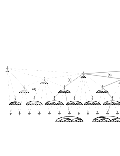
The periodic time series of period $q$ that constitutes the trajectory within an attractor with $\omega(\Omega)=p/q$ is represented in the HV graph by the repeated concatenation of a motif, a number of which are shown in Fig. 1. The display of these motifs in the Farey tree in Fig. 1 helps visualize the inflationary process that takes place when the HV network grows at the onset of chaos luque6 . For illustrative purposes in Fig. 1 we show the periodic motifs of the HV graphs that are associated with the irreducible rational numbers $p/q\in[0,1]$, and we place them on the Farey tree hilborn1 along which routes to chaos take place. A well-studied case is the sequence of rational approximations of $\omega_{\infty}=\phi^{-1}=(\surd 5-1)/2=0.618034...$ , the reciprocal of the golden ratio, which yields winding numbers $\{\omega_{n}=F_{n-1}/F_{n}\}_{n=1,2,3...}$ where $F_{n}$ is the Fibonacci number generated by the recurrence $F_{n}=F_{n-1}+F_{n-2}$ with $F_{0}=1$ and $F_{1}=1$. The first few steps of this route can be seen in Fig. 1(b).

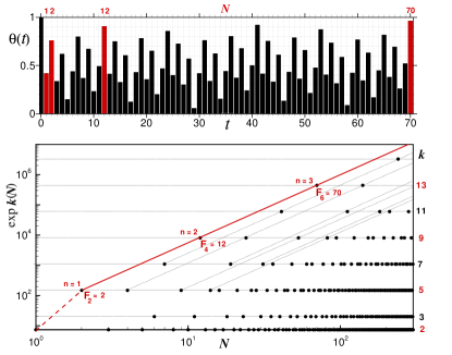
The trajectories generated by the map with initial condition $\theta_{0}=1$ at the golden ratio onset of chaos define a multifractal attractor that forms a striped pattern of positions when plotted in logarithmic scales, i.e. $\ln\theta_{t}$ vs $\ln t$. See Fig. 3 in Ref. robledo1 . This attractor corresponds to the accumulation point $\Omega_{\infty}=\lim_{n\rightarrow\infty}\Omega_{n}$ of bare winding numbers $\Omega_{n}$ that characterize superstable trajectories of periods $F_{n}$, $n=1,2,3,...$, $\Omega_{\infty}=0.606661...$ robledo1 . A sample of this time series is shown in the top panel of Fig. 2. In the bottom panel of the same figure we plot, in logarithmic scales, the outcome of the HV method with use of the variable $\exp k(N)$, where $k(N)$ is the degree of node $N$ in the graph generated by the time series $\theta_{t}$ (that is, $N\equiv t=1,2,3,...$). Notice that the distinctive striped pattern of the attractor robledo1 is present in the figure, although in a simplified manner where the fine structure is replaced by single lines of constant degree. The HV algorithm transforms the multifractal attractor into a discrete set of connectivities.

III Diagonal structure of the connectivity fluctuations

It is clear from the bottom panel of Fig. 2 that the degree $k(N)$, and also $\exp k(N)$, fluctuates when $N$ is increased step by step via a deterministic pattern of ever increasing amplitude. Notice also in the same panel the diagonal lines that are drawn to connect sequences of node-connectivity ($N,k$) values; there is a main diagonal followed by two other diagonals close to each other. These ($N,k$) sequences fall asymptotically along parallel straight lines, that begin after the initial steps from the lowest values of the degree, $k=2$ or $k=3$, skip the absent $k=4$, and reach the values $k=5$ or $k=6$, and therefore the sequences obey a power law with the same exponent. There are many more sequences along same-slope diagonals, not highlighted in the figure, arranged in close groups and that trace all other possible connectivities $k(N)$. See also Fig. 3 in Ref. robledo1 . It is by examining the dependence of $k(N)$ along each member of this family of diagonals that the scaling and entropic properties of the network are determined.

Figure 2: Top: Positions $\theta_{t}$ as a function of ${\small t}$ for the first ${\small 55}$ data for the orbit with initial condition ${\small\theta}_{0}{\small=1}$ at the golden ratio onset of chaos (see text) of the critical circle map ${\small K=1}$. The data highlighted are associated with specific subsequences of nodes (see text). Bottom: Log-log plot of ${\small\exp k(N)}$ as a function of the node $N$ for the HV graph generated from same time series as as for the upper panel but for $3\times 10^{2}$ iterations, where ${\small N=t}$. The distinctive band pattern of the attractor manifests through a pattern of single lines of constant degree. The node positions of some node subsequences along diagonals is highlighted as guide lines to the eye. The inset shows the collapse of all nodes in the graph into a single diagonal (see text).

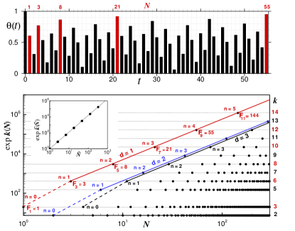
Thus, the ($N,k$) pairs in the graph define a structure in diagonals $d=1,2,3,...$, and on each diagonal $d$ we label the particular nodes that lie on it as $n=0,1,2,...$ Thus, $N(n;d)$ indicates the node/time for the $n$-th position on diagonal $d$. For example, in the first and main diagonal $d=1$ in Fig. 2 we have $N(0;1)=1=F_{1}$, $N(1;1)=3=F_{3}$, $N(2;1)=8=F_{5}$, $N(3;1)=21=F_{7}$,… As it can be seen in the top panel of Fig. 2, the matching positions $\theta_{t}$, $t=F_{2n+1}$ (highlighted) grow monotonically when removed from the rest of the time series, and according to the HV algorithm this implies increasing values for the degrees of their corresponding nodes. For $d=2$ (the second diagonal in Fig. 2) $N(0;2)=2$, $N(1;2)=6$, $N(2;2)=16$, $N(3;2)=42$,… All the nodes $N(n;d)$ can be expressed via the recurrence formula

$$N(0;d) = \textrm{mex}\{N(n;i):1\leq i<d,n\geq 0\},$$

$$N(1;d) = 2N(0;d)+d,$$

$$N(n;d) = 3N(n-1;d)-N(n-2;d),$$ (2)

with $d=1,2,...$ and $n=0,1,2,..$., where the term mex stands for MinimumEXclude value conway1 that in this case it means the smallest value of $N$ that has not appeared in the previous diagonals. In fraenkel1 it is demonstrated that every integer $N$ appears only once under the above recurrence and this exotic enumeration occurs in a natural way  in the golden ratio route. In fact, all the time labels $n$ along the diagonals $d=1,2,...$ can be expressed as Fibonacci numbers $F_{n}^{(d)}=F_{n-1}^{(d)}+F_{n-2}^{(d)}$ with different initial conditions for each one of them,

$$F_{0}^{(d)} = d,\ F_{1}^{(d)}=N(0;d),$$

$$N(n;d) = F_{2n+1}^{(d)}.$$ (3)

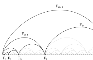
This recurrence is the consequence of the inflationary process that takes place in the generation of graphs via the golden ratio route luque6 . Notice that this route goes through successive approximants of the continued fraction $[1,1,1,...]$ (see Fig. 1b). These approximants permanently alternate from larger to smaller to larger values around the golden number, such that an approximant graph is generated by concatenation of the two preceding approximant graphs alternating the order of concatenation at each stage. This can be seen explicitly in Fig. 3.

Figure 3: First substructures of the quasiperiodic graph associated with the golden ratio route to chaos. The resulting patterns follow from the universal order with which an orbit visits the positions of the attractor. The quasiperiodic graph associated with the time series generated at the onset of chaos ($n\rightarrow\infty$) is the result of an infinite application of the inflationary process by which a graph at period $F_{2n+1}$ is generated out of graphs at periods $F_{2n}$ and $F_{2n-1}$ luque6 . The first few node/time steps along the first diagonal ($d=1$) are highlighted.

The recurrence formula in Eq. (2) can be solved leading to an explicit expression convenient for our purposes. First, it can be demonstrated fraenkel1 that

$$N(0;d) = \lfloor(d-1)\phi\rfloor+1,$$

$$N(n;d) = \lfloor N(n-1;d)\phi^{2}\rfloor+1.$$ (4)

Then, use of the approximation $N(n;d)\approx N(n-1;d)\phi^{2}$ and of the definition $C_{d}\equiv N(1;d)=\big{\lfloor}(\lfloor(d-1)\phi\rfloor+1)\phi^{2}\big{\rfloor}+1$ yields the solution

$$N(n;d)=C_{d}\phi^{2n-2},\ n\geq 1.$$ (5)

This equation captures the values $N(n;d)$ along the diagonals starting always from $n=1$, that, as we can observe in the bottom panel of Fig. 2, are the nodes with connectivities $k=5$ or $k=6$. Furthermore, all the (parallel straight- line) diagonals can be collapsed into a single one by first redefining the connectivities in each of them such that the degree is zero in the initial position $n=1$. To do this it is only necessary to subtract $5$ or $6$ according to the given diagonal, with the outcome that $\widetilde{k}=2n-2$ with $n=1,2,...$ To get the collapse it is sufficient to introduce the change of variable $\widetilde{N}(n;d)=N(n;d)/C_{d}$ so that $\widetilde{N}(n;d)=\phi^{2n-2}$. We can see the result in the inset in the bottom panel of Fig. 2. To keep notation simple we make use of this variable and write $k$ instead of $\widetilde{k}$ from now on.

Figure 4: Log-log plot of the distance between two nearby trajectories $l_{t}=|\theta_{t}-\theta_{t}^{\prime}|$ close to ${\small\theta}_{0}{\small=1}$, where ${\small l}_{0}{\small=10}^{-4}$, measured at times ${\small t=N(n;d)}$, ${\small n=0,1,2,...}$, along the main diagonal ${\small d=1}$ at the transition to chaos for the golden, silver and bronze routes (see text).

IV Generalized Lyapunov exponents at the accumulation point of the golden ratio route to chaos

We define now a connectivity expansion rate for the graph under study. The formal network analog of the sensitivity to initial conditions in the map is luque5

$$\xi(N(n;d))\equiv\frac{\exp(k(n))}{\exp(k(1))}=\exp(k(n)),$$ (6)

since $k(1)=k(N(1;d))=0$. That is, we compare the expansion $\exp(k(n))$ with the minimal $\exp(k(1))=1$ occurring always at nodes at positions $N(1;d)$.

From Eq. (5) we have

$$k(N(n;d))=2n-2=\ln\left(\frac{N}{C_{d}}\right)^{\frac{1}{\ln\phi}},$$ (7)

or

$$\xi(N(n;d))=\left(\frac{N}{C_{d}}\right)^{\frac{1}{\ln\phi}}.$$ (8)

The standard network Lyapunov exponent is defined as

$$\lambda\equiv\lim_{N\rightarrow\infty}\frac{1}{N}\ln\xi(N),$$ (9)

but since Eq. (8) indicates that the bounds of the fluctuations of $\xi(N)$ grow with $N$ slower than $\exp N$ we have $\lambda=0$, in agreement to the ordinary Lyapunov exponent at the onset of chaos.

To get a suitable expansion rate that grows linearly with the size of the network, we deform the ordinary logarithm in $\ln{\xi(N)}=k(N)$ into $\ln_{q}\xi(N)$ by an amount $q>1$ such that $\ln_{q}\xi(N)$ depends linearly in $N$, where $\ln_{q}x\equiv(x^{1-q}-1)/(1-q)$ and $\ln x$ is restored in the limit $q\rightarrow 1$ Koelink ; robledo2 . And through this deformation we define the generalized graph-theoretical Lyapunov exponent as

$$\lambda_{q}\equiv\frac{1}{\Delta N}\ln_{q}\xi(N),$$ (10)

where $\Delta N=N(n;d)-C_{d}$ is the node distance or iteration time duration between an initial node $N(1;d)$ where $d$ is fixed and $N(n;d)$ is the final node position. From Eq. (8) we obtain

$$\lambda_{q}(d)=\frac{1}{N-C_{d}}\frac{\left(\frac{N}{C_{d}}\right)^{\frac{1-q}{\ln\phi}}-1}{1-q}=\frac{1}{C_{d}\ln\phi},$$ (11)

where the degree of deformation $q$ is found to be $q=1-\ln\phi$. This way we have determined a spectrum of generalized Lyapunov exponents $\lambda_{q}(d)$, one for each diagonal $d=1,2,...$ in Fig.2. The largest value is for the main diagonal, $\lambda_{q}(1)=(C_{1}\ln\phi)^{-1}$, and the others gradually decrease as $d\rightarrow\infty$.

V $q$-deformed entropy expression and Pesin-like identities

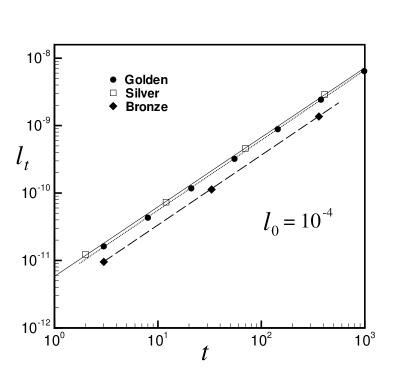
Having obtained the family of generalized Lyapunov exponents $\lambda_{q}(d)$ from a suitable expansion rate $\ln_{q}\xi(N)$, we proceed to analyze the entropic properties of the network. At the transition to chaos for the golden ratio the HV method creates a single network that represents many different trajectories. Trajectories initiated at different positions of the attractor produce networks related to each other by a node translation equal to the number of iterations needed from one initial position $\theta_{0}^{(1)}$ to reach the second $\theta_{0}^{(2)}$. The two positions appear in the trajectory initiated at $\theta_{0}=0$ at times $t_{1}$ and $t_{2}$, $\theta_{0}^{(1)}=\theta_{t_{1}}$ and $\theta_{0}^{(2)}=\theta_{t_{2}}$, and the node translation is $\delta N=t_{2}-t_{1}>0$. This shift property can be visualized in Fig. 2, and is implicated in the derivation of Eq. (10) for $\lambda_{q}(d)$. But also, trajectories initiated at positions off the attractor, but sufficiently close to a position of this set generate the same network, as the HV method distinguishes differences in trajectory positions only when they surpass threshold values. There is a basic property of trajectories at the onset of chaos that combines with the previous remark and that can be used to describe the rate of entropy growth of the network with its size. This property is that for a small interval of length $l_{0}$ with $\mathcal{N}$ uniformly-distributed initial conditions around, say, $\theta_{0}=0$, all trajectories behave similarly, remain uniformly-distributed at later times and follow the concerted pattern shown in Fig. 3 in Ref. robledo1 . Studies of entropy growth associated with an initial distribution of positions with iteration time $t$ of several chaotic maps latora1 have established that a linear growth occurs during an intermediate stage in the evolution of the entropy, after an initial transient dependent on the initial distribution and before an asymptotic approach to a constant equilibrium value. In relation to this it was found, both at the period-doubling baldovin1 ; mayoral1 and at the quasiperiodic golden ratio robledo1 transitions to chaos, that (i) there is no initial transient if the initial distribution is uniform and defined around a small interval of an attractor position, and (ii) the distribution remains uniform for an extended period of time due to the subexponential dynamics. In Fig. 4 we demonstrate this property by presenting the time evolution of the distance between to nearby trajectories, say the endpoints of the interval of length $l_{t}$ containing the $\mathcal{N}$ uniformly-distributed positions at time $t$, for the golden ratio transition to chaos, and also for other quasiperiodic transitions to chaos along other routes discussed below. But the time evolution of the trajectory distances in Fig. 4 can also be that between any pair of adjacent positions in the initial uniform distribution and therefore the trajectories distribution remains uniform after continued iterations.

We denote the above-referred distribution by $\pi(t)=1/W(t)$ where $W(0)=l_{0}/\mathcal{N}$ is the number of cells that cover the initial interval $l_{0}$. As stated, all such trajectories give rise to the same HV graph, and at iteration times, say, of the form $t=N(n;d)$, $n=1,2,3,\dots$, the HV criterion assigns $k=2n-2$ links to the common node $N(n;d)$. The distribution $\pi$ is defined in the map but we can look at its $n$-dependence, $\pi(N(n;d))$, if the scaling properties of the network retain the scaling property of $\pi$ in the map. We can corroborate this and also that the entropic properties derived from this distribution are connected to the network Lyapunov exponents described in the previous section. The scaling property of the network that yields the collapse of the diagonals in Fig. 2 described above implies that the uniform distributions $\pi$ for the consecutive node-connectivity pairs ($N(n;d),2n-2$) and ($N(n+1;d),2(n+1)-2$) along the same diagonal $d$ scale with the same factors and this leads us to conclude that the $n$-dependence for these distributions is

$$\pi(N)=W_{n}^{-1}=\exp(-2n+2).$$ (12)

But since

$$W_{n}=\exp(2n-2)=\left(\frac{N}{C_{d}}\right)^{\frac{1}{\ln\phi}},$$ (13)

the ordinary entropy associated with $\pi$ grows logarithmically with the number of nodes $N$, $S_{1}\left[\pi(N)\right]=\ln W_{j}\sim\ln N$. However, the $q$-deformed entropy

$$S_{q}\left[\pi(N)\right]\equiv\ln_{q}W_{n}=\frac{1}{1-q}\left[W_{n}^{1-q}-1\right],$$ (14)

where the amount of deformation $q$ of the logarithm has the same value as before, grows linearly with $N$, as $W_{n}$ can be rewritten as

$$W_{n}=\exp_{q}[\lambda_{q}\Delta N],$$ (15)

with $q=1-\ln\phi$ and $\lambda_{q}(d)=(C_{d}\ln\phi)^{-1}$. Therefore, if we define the entropy growth rate

$$h_{q}\left[\pi(N)\right]\equiv\frac{1}{\Delta N}S_{q}\left[\pi(N)\right]$$ (16)

we obtain

$$h_{q}\left[\pi(N)\right]=\lambda_{q}(d),$$ (17)

a Pesin-like identity at the onset of chaos (effectively one identity for each subsequence of node numbers , $n=1,2,3,\dots$, given each by a value of $d=1,2,3,...$).

Figure 5: Top: Positions $\theta_{t}$ as a function of ${\small t}$ for the first ${\small 70}$ data for the orbit with initial condition ${\small\theta}_{0}{\small=1}$ at the silver number onset of chaos (see text) of the critical circle map ${\small K=1}$. The data highlighted are associated with specific subsequences of nodes (see text). Bottom: Log-log plot of ${\small\exp k(N)}$ as a function of the node ${\small N}$ for the HV graph generated from same time series as as for the upper panel but for $3\times 10^{2}$ iterations, where ${\small N=t}$. The distinctive band pattern of the attractor manifests through a pattern of single lines of constant degree. The node positions of some node subsequences along diagonals is highlighted as guide lines to the eye.

VI Quasiperiodic graphs at the onset of chaos for quadratic irrationals

We can generalize the above results for every quadratic irrational in $[0,1]$ with pure periodic continued fraction representation: $\phi_{b}^{-1}=[b,b,b,...]=[\overline{b}]$ ($b=1$ , $2$, $3$, correspond to the golden, silver and bronze routes, respectively). These irrationals are the solutions of the equation $x^{2}-bx-1=0$, where $b$ is a natural number. The dressed winding number is now $\omega_{\infty}=\lim_{n\rightarrow\infty}[1-(F_{n-1}/F_{n})]=\phi_{b}^{-1}$with $F_{n}=bF_{n-1}+F_{n-2}$, $F_{0}=0$, $F_{1}=1$ and the route to chaos is the infinite sequence of attractors with periods $F_{n}$, $n=1,2,3,...$(Notice now $F_{n}$ is only a Fibonacci number when $b=1$). The first few steps of the silver route $b=2$ can be seen in Fig. 1(c), whereas Fig. 5 shows results for the attractor at the onset of chaos via this route. Similarly to Fig. 2 for $b=1$, in the top panel of Fig. 5 is the time series for the first $70$ iteration times, while in the bottom panel of the same figure we plot, in logarithmic scales, the outcome of the HV method with use of the variable $\exp k(N)$. As it can be observed the networks for the two cases are qualitatively similar, although there are differences, mainly the absence of even connectivities when $k>5$.

This absence can be verified by inspection of the degree distribution $P_{\infty}(k)$ for the graphs at the $\omega_{\infty}=\phi_{b}^{-1}$ accumulation points luque6

$$P_{\infty}(k)=\left\{\begin{array}[]{ll}\phi_{b}^{-1}&k=2\\ 1-2\phi_{b}^{-1}&k=3\\ (1-\phi_{b}^{-1})\phi_{b}^{(3-k)/b}&k=bn+3,\;n\in\mathbb{N}\\ 0&\mathrm{otherwise,}\end{array}\right.$$ (18)

where we can see explicitly which values of $k$ are not present for a given value of $b$. This and other connectivity properties can be worked out from the inflation process of the graphs. See Fig. 6.

Figure 6: First substructures of the quasiperiodic graph associated to (a) the silver number ${\small b=2}$ and (b) the bronze number ${\small b=3}$ routes to chaos. The resulting patterns follow from the universal order with which an orbit visits the positions of the attractors. The quasiperiodic graph associated with the time series generated at the onset of chaos ($n\rightarrow\infty$) is the result of an infinite application of the inflationary process by which a graph at period $F_{2n}$ is generated out of graphs at periods $F_{2n-2}$ and $F_{2n-1}$ luque6 .

We will center our attention on the first diagonal $d=1$. For every $b$, the node positions on the first diagonal, $n=1,2,3,...$, are

$$N(n;1)=F_{2n},$$ (19)

that with the use of the generalized Binet formula

$$F_{n}=\frac{1}{\sqrt{b^{2}+4}}\left[\phi_{b}^{n}-\left(\frac{-1}{\phi_{b}}\right)^{n}\right]\approx\frac{\phi_{b}^{n}}{\sqrt{b^{2}+4}},$$

can be written as

$$N(n;1)\approx\frac{1}{\sqrt{b^{2}+4}}\phi_{b}^{2n}=\frac{1}{\sqrt{b^{2}+4}}\phi_{b}^{2}\phi_{b}^{2n-2}=C_{b}\phi_{b}^{2n-4},$$ (20)

where the position $n=1$ is

$$N(1;1)=F_{2}\approx\frac{1}{\sqrt{b^{2}+4}}\phi_{b}^{2}\equiv C_{b}.$$ (21)

We note that the connectivity of the first node is $k(n=1)=b+3$ and in general $k(n)=b+3+2b(n-1)$, $n\geq 2$. As before we redefine the connectivities such that the degree is zero at the initial position $n=1$, $k(n)=2b(n-1)$, $n=1,2,3,...$ Following the same procedure as in Section 4, from Eq. (20) we have

$$k(N(n;1))=2b(n-1)=\ln\left(\frac{N}{C_{b}}\right)^{\frac{1}{\ln\phi_{b}}},$$ (22)

and use of it in the sensitivity $\xi(N(n;1))\equiv\exp(k(n))$ yields

$$\xi(N(n;1))=\left(\frac{N}{C_{b}}\right)^{\frac{1}{\ln\phi_{b}}}.$$ (23)

Since all the features required for the $q$-deformation described in Section 4 are present for general $b$, we obtain for the generalized Lyapunov exponent the expression

$$\lambda_{q}^{(b)}(1)=\frac{1}{N-C_{b}}\frac{\left(\frac{N}{C_{b}}\right)^{\frac{1-q}{\ln\phi_{b}}}-1}{1-q}=\frac{1}{C_{b}\ln\phi_{b}},$$ (24)

where $q=1-\ln\phi_{b}$. Likewise, the contents of Section 5 can also be reproduced for general $b$ with the result that

$$h_{q}\left[\pi(N)\right]=\lambda_{q}^{(b)}(1).$$ (25)

VII Summary and discussion

At the quasiperiodic onset of chaos the HV method leads to a self-similar network with a structure illustrated by the related periodic networks obtained from the sequence of attractors of finite periods along the route to chaos luque6 . Under the HV algorithm many nearby trajectory positions lead to the same network, since only when the values of trajectory positions cross a threshold the corresponding node increases its degree with new links. (See the succinct definition of the algorithm and the top panel in Fig. 2). Therefore trajectories off the attractor but close to it transform into the same network structure. As we have seen the fluctuations of the degree capture the anomalous but basic behavior of the fluctuations of the sensitivity to initial conditions at the transition to chaos robledo1 . The graph-theoretical analogue of the sensitivity was identified as $\exp(k)$ while the amplitude of the variations of $k$ grows logarithmically with the number of nodes $N$. These deterministic fluctuations are described by a discrete spectrum of generalized graph-theoretical Lyapunov exponents that are shown to relate to an equivalent spectrum of generalized entropy growth rates, yielding a set of Pesin-like identities. This behavior is similar to what was observed for the case of the more straightforward period-doubling accumulation point luque5 . The definitions of these quantities involve a scalar deformation of the ordinary logarithmic function that ensures their linear growth with the number of nodes. Therefore the entropy expression involved is extensive and of the Tsallis type with a precisely fixed value of the deformation index $q$, $q=1-\ln\phi_{b}$, where $\phi_{b}$ is the inverse of the irrational (dressed) winding number.

We have considered special families of time series and converted each into a network, each family consists of the trajectories associated with an attractor at the quasiperiodic transition to chaos of circle maps. The attractors studied are defined by a winding number given by a quadratic irrational or, equivalently, by a pure periodic continued fraction. Each winding number singles out a specific route to chaos. Amongst these we described in some detail the so-called golden route, but also we have shown results for those known as the silver and bronze routes luque6 . See Figs. 1 and 4. The HV algorithm proved to be capable of generating a single network that contains the scaling and entropic properties of the trajectories associated with each attractor. The results presented here are of the same kind as those obtained for the period-doubling route to chaos luque5 suggesting that the HV networks associated with the onset of chaos are useful for describing the universal properties at these special systems. The Pesin identity is a reflection of a basic connection between BG statistical mechanics and chaos so that our results provide elements for an analogous connection for the case of nonergodic and nonmixing dynamics at vanishing ordinary Lyapunov exponent.

Acknowledgements.  We acknowledge financial support by the Comunidad de Madrid (Spain) through Project No. S2009ESP-1691 (B.L.), support from CONACyT & DGAPA (PAPIIT IN100311)-UNAM (Mexican agencies) (A.R.).

References

- (1) S.H. Strogatz, Nonlinear Dynamics and Chaos: With Applications to Physics, Biology, Chemistry, and Engineering, Perseus Books Publishing, LLC, Reading, 1994.
- (2) J.R. Dorfman, An Introduction to Chaos in Nonequilibrium Statistical Mechanics, Cambridge University Press, Cambridge, 1999.
- (3) L. Lacasa, B. Luque, F. Ballesteros, J. Luque, J.C. Nuño, Proc. Natl. Acad. Sci. USA 105 (2008) 4973.
- (4) B. Luque, L. Lacasa, J. Luque, F. Ballesteros, Phys. Rev. E 80 (2009) 046103.
- (5) B. Luque, L. Lacasa, F. Ballesteros, A. Robledo, PLoS ONE 6 (9) (2011).
- (6) B. Luque, L. Lacasa, F. Ballesteros, A. Robledo, Chaos 22 (2012) 013109.
- (7) B. Luque, L. Lacasa, A. Robledo, Phys. Lett. A 376, 362 (2012).
- (8) B. Luque, A.M. Núñez, F. Ballesteros, A. Robledo, J. Nonlinear Sci. 23, 335 (2013).
- (9) A.M. Núñez, B. Luque, L. Lacasa, J. P. Gómez, A. Robledo, Phys. Rev. E 87, 052801 (2013).
- (10) R.C. Hilborn: Chaos and Nonlinear Dynamics. Oxford University Press, New York (1994).
- (11) F. Baldovin, A. Robledo, Phys. Rev. E 69 (2004) 045202(R).
- (12) E. Mayoral, A. Robledo, Phys. Rev. E 72 (2005) 026209.
- (13) Y.B. Pesin, Russian Math. Surveys 32 (1977) 114.
- (14) J.P. Crutchfield, K. Young, Phys.Rev. Lett. 63, 105 (1989).
- (15) J. Zhang, M. Small, Phys. Rev. Lett. 96, 238701 (2006).
- (16) F. Kyriakopoulos and S. Thurner, Lect. Notes in Comput. Sci. 4488, 625 (2007).
- (17) X. Xu, J. Zhang, and M. Small, Proc. Natl. Acad. Sci. USA, 105, 19601 (2008).
- (18) R. V. Donner, Y. Zou, J. F. Donges, N. Marwan, and J. Kurths, New J. Phys. 12, 033025 (2010).
- (19) R. V. Donner et al., Int. J. Bif. Chaos 21, 1019 (2010)
- (20) R. V. Donner et al., Eur. Phys. J. B 84, 4, 653 (2011).
- (21) A. S. L. O. Campanharo, M. I. Sirer, R. D. Malmgren, F. M. Ramos, L. A. N.Amaral, PLoS ONE 6 (2011).
- (22) H. Hernández-Saldaña, A. Robledo, Physica A370, 286 (2006).
- (23) C. Bandt, B. Pompe, Phys. Rev. Lett. 88 (2002) 174102.
- (24) L.D. Landau, Dokl. Akad. Nauk SSSR 44, 339 (1944).
- (25) D. Ruelle and F. Takens, Commun. Math. Phys. 20, 167 (1971).
- (26) S.J. Shenker, Physica D 5, 405 (1982).
- (27) M.J. Feigenbaum, L.P. Kadanoff, and S.J. Shenker, Physica D 5, 370 (1982).
- (28) D. Rand, S. Ostlund, J. Sethna, and E.D. Siggia, Phys. Rev. Lett. 49, 132 (1982).
- (29) D. Rand, S. Ostlund, J. Sethna, and E.D. Siggia, Physica D 8, 303 (1983).
- (30) E.R. Berlekamp, J.H. Conway and R.K. Guy (1982), Winning Ways (two volumes), Academic Press, London.
- (31) A. S. Fraenkel, Theoretical Computer Science 282 (2002) 271 284.
- (32) E. Koelink, W. van Assche, Proc. AMS 137, 5 (2009) 1663-1676.
- (33) A. Robledo, Physica A 370, 449 (2006).
- (34) V. Latora, M. Baranger, Phys. Rev. Lett. 82 (1999) 520.