Quantum repeater with Rydberg blocked atomic ensembles in fiber-coupled cavities
Abstract
We propose and analyze a quantum repeater architecture in which Rydberg blocked atomic ensembles inside optical cavities are linked by optical fibers. Entanglement generation, swapping and purification are achieved through collective laser manipulations of the ensembles and photon transmission. Successful transmission and storage of entanglement are heralded by ionization events rather than by photon detection signal used in previous proposals. We demonstrate how the high charge detection efficiency allows for a shortened average entanglement generation time, and we analyze an implementation of our scheme with ensembles of Cs atoms.
pacs:
03.67.Hk, 32.80.Ee, 42.50.ExI Introduction
A possible route towards scalable quantum computers and quantum communication networks combines small quantum processor nodes which communicate via the exchange of moving information carriers, the so-called flying qubits, which will typically be photons. The direct exchange of a photon, either through free space or a fiber, between a pair of nodes does not have unit success probability, and to safely communicate quantum states, one can instead apply entangled state in teleportation protocols B93 ; B96 , where the entanglement of two remote nodes can be achieved, e.g. after multiple attempts until a suitable heralding detection event certifies the establishment of the state. For long distances, photon loss makes the success probability small, and hence the average time needed to establish a state for transmission of a single bit of quantum informsation very long. This problem, however, can be solved by the quantum repeater setup BDCZ98 which divides the transmission path between the nodes into smaller segments with auxiliary nodes over which losses are strongly diminished. The auxiliary nodes are first entangled with their nearest neighbors in a heralded way followed by a succession of local measurements which cause the graduate projection on quantum states with entanglement distributed over longer and longer distances (entanglement swapping). The implementation of this approach is compatible with different physical setups involving atomic ensembles and linear optical operations. The most influential proposal is the so-called DLCZ protocol DLCZ01 , whose feasibility was experimentally considered in its two-node version in KBBDCDBK03 .
This manuscript presents a quantum repeater scenario, based on the Rydberg blockade phenomenon. Rydberg blockade refers to the strong dipole-dipole interaction between pairs of highly excited atoms, which after laser excitation of a single atom shifts the resonance condition for all the other atoms and hence blocks further excitation by the laser field. Rydberg blockade forbids the resonant excitation of more than one Rydberg atom in an atomic mesoscopic sample CP10 , and has been experimentally observed, e.g., in VVZCCP06 ; UJHIYWS09 . In JCZRCL00 it was proposed to take advantage of Rydberg blockade in quantum information processing, leading to an intensive current field of research SWM10 . Different theoretical proposals have been recently put forward, which allow to take advantage of the full spectroscopic richness of Rydberg interactions for quantum information purposes BMM07 ; BPMCS07 ; BPM07 , and a novel framework for quantum information encoding and computing has been proposed LFCD01 ; BMS07 ; BPSM08 ; SWM10 , in which register qubit states are physically implemented by the (symmetric) occupational states of internal atomic levels in an ensemble of ) identical atoms.
The collective laser manipulation of the system combined with the Rydberg blocking interaction allows one to store and universally process information in the subspace of symmetric ensemble states containing at most one atom in each internal level. The primary advantage of ensembles over single atoms consists in their enhanced coupling to external control fields, which allows for efficient and rapid processing. A secondary practical advantage is that even in a multi-qubit register, one merely needs to address the atoms collectively, contrary to individual-atom encoding of qubits which requires the precise control of each and every single particle in the system.
In the quantum repeater we propose here, the nodes are identical atomic ensembles, placed in cavities which are linked via optical fibers. The internal structure of the atoms is such that each ensemble accomodates three logical subnodes, called the left , the right , and the auxiliary subnode in the following. In the first step of our protocol, we entangle the logical state of the subnode in the cavity with the polarization state of a single photon released in the cavity. This photon is then transmitted to the neighboring cavity where it is absorbed by the left subnode degree of freedom of the atomic ensemble in that cavity, which thus becomes entangled with . A conditional gate applied to subnodes and , followed by appropriate ionization detection is used to ensure that no error occurred during the entanglement generation, in particular that the photon was not lost during the transfer through the fiber between the cavities. If needed, subnodes are reset so that the entanglement generation operation can be repeated until successful. Once all pairs have been correctly entangled, entanglement is swapped by ensemble operations on every pair . Measurements using Rydberg blockade and ionization detection on all subnodes finally heralds the entangled state of the remote pair which can be transformed into any required Bell state by application of a unitary operation on prescribed by the results of the measurements. If one of the measurements fails, the procedure must be repeated.
We note that the use of Rydberg blocked ensembles as quantum repeaters has been proposed in ZMHZ10 ; HHHLS10 . Though related our proposal, however, never makes use of photon detection to generate entanglement between neighbouring nodes, we solely rely on ensemble laser manipulations (including ionizing pulses), ion detection whose efficiency can be made very close to one , and photon transmissions through optical fibers. This allows for a shortened entanglement generation average time whose expression is derived in the Appendix.
The paper is structured as follows. In Sec. II, we present our quantum repeater scheme using Rydberg blockaded ensembles in optical cavities coupled by optical fibers. In Sec. III, we analyze the different steps of our protocol with emphasis on their robustness against errors, and we compute the average duration of our scheme. In Sec. IV, we suggest a physical implementation. In Sec. V, we compare our scheme with other schemes for quantum repeaters, and we conclude in Sec. VI.
II The model
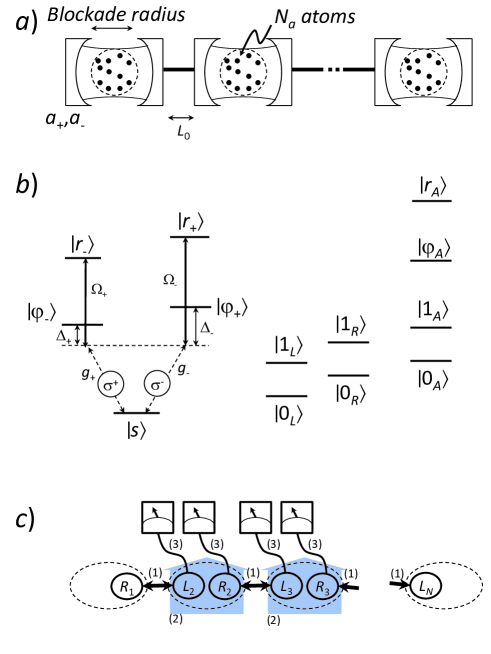
Our quantum repeater setup consists of atomic ensembles placed in cavities which are linked by optical fibers (see Fig. 1a). Neighboring cavities are separated by the distance .
The atomic level structure is represented in Fig. 1b. All the atoms are initially prepared in the “reservoir” state , and the atoms have, in addition, six metastable states denoted by , three excited states and three high-lying Rydberg states . We assume that the transitions given in Table 1 can be independently and selectively addressed by appropriately tuned laser beams. In particular, it implies that we can couple pairs of states, , , and via the intermediate states , or .
We further suppose that the atomic samples are small enough to operate in the full Rydberg blockade regime, their size should not exceed a few m. As a consequence, when driving the transition on a sample with atoms initially in the state , multiply excited states are out of resonance due to the strong dipole-dipole interaction among Rydberg excited atoms, and the transfer of more than a single atom to the Rydberg state is blocked. The fields are applied symmetrically to all atoms in each sample, and they hence excite the symmetric collective state with a single Rydberg excitation, . The associated coupling strength is easily seen to be magnified by the factor with respect to the coupling strength of the single atom transition . Applying a pulse on the collective ensemble transition, followed by the single-particle transition , prepares the sample in a stable symmetric collective state where the ’s denote the populations of the different internal levels, restricted to values and . Unitary operations can be applied in the eight-dimensional subspace of collective states, , by simply driving the corresponding single-atom transitions and/or , as described in BMS07 ; BPM07 . The collective state pairs (), (), and () at each repeater node can thus be associated with three qubits, referred to as the left , right and auxiliary subnodes, in the following.
We shall use a simplified notation for ensemble states, denoting the collective internal state population as and , such that, e.g., denotes the state , where both the right and the auxiliary subnodes occupy the logic state 1, while the left subnode is in state .
It is a further requirement of our protocol that the transitions couple non-resonantly to two different modes, , with equal frequency and with detunings with respect to the atomic transitions, but different polarization in the cavity (this will legitimate the assumptions we make below on the fiber transmission/losses). Driving the upper transition with a laser field with detuning and Rabi frequency , induces a second-order quantum-classical process, described by the single-atom effective Hamiltonian where denotes the annihilation operator of the cavity mode and its coupling strength. This Hamiltonian derives from the adiabatic elimination of the intermediate state BPM07-1 , and is valid for . Performing an ensemble pulse on the quantum-classical two-photon transition hence converts a collective Rydberg excitation into a cavity photon and the other way around, with the coupling strength . We emphasize that, though only a single cavity photon is emitted/absorbed during the process, the coupling can be made strong, thanks to the atomic ensemble magnification factor GBEM10 . To avoid spurious interference effects we suggest to apply different detuning parameters for the two transitions proceeding via the same intermediate state .
Optical fibers P97 couple the cavities to each other, and we simply assume that the fiber between two neighboring cavities achieves the coupling
| (1) |
with a coupling strength between the modes in the cavity with annihilation operator , and the same modes in the cavity. Since the modes differ by their polarizations but have the same frequency, we make the reasonable assumption that the ’s have the same value for all . We moreover suppose that the coupling between two neighboring cavities can be switched on and off, for instance by a controlled Pockels cell : this will allow us to isolate and separately deal with pairs of coupled nodes.
Due to fiber loss, the transmission of a photon from one cavity to its neighbor is not perfect. We shall assume that the transmission efficiency is the same for all fiber connections and can be written under the form where is the attenuation length, typically of the order of km (corresponding to losses of dB/km). The probability for loosing one photon during the transmission along a fiber mode of length is thus given by .
III The scheme
In this section, we describe how to entangle two remote nodes using the model we presented in the previous section. First, we briefly sketch the different steps of our scheme in the ideal case without losses. Then, we show how to make our method immune to photon loss and spontaneous emission from the Rydberg level. Finally, we analyze the effects of other possible errors on the performance of our protocol.
III.1 The different steps of the scheme
Initially, all the cavities are empty and all ensemble atoms are in the reservoir state . The first step consists in entangling pairs of neighboring subnodes (see Fig. 1c). To this end, one applies the sequence of operations given in Table 2. In this table, dashed-line arrows are used for non-resonant couplings to the intermediate states. Moreover, the “ensemble” nature of pulses is emphasized by a factor above the concerned arrows. Finally, we indicate when a cavity mode is involved in a transition by writing “single photon ” above the corresponding arrow.
| i) simultaneous pulses (same Rabi frequency) on ensemble |
| ii) pulse on ensemble |
| iii) pulse on ensemble |
| iv) pulse on ensemble |
| v) pulse on ensemble |
| vi) pulse on ensemble |
| vii) pulse on ensemble |
| viii) Transfer of the photon through the fiber |
| from cavity to cavity |
| ix) pulse on ensemble |
| x) pulse on ensemble |
| xi) pulse on ensemble |
| xii) pulse on ensemble |
The first seven pulses in Table 2 prepare the subnode and the cavity in the entangled state where denotes the number state of the cavity mode . The photon thus released is then transferred to the cavity through the fiber (step ). The last four pulses of the sequence translate the photonic excitation into an atomic excitation of the ensemble : a “” photon is translated into a excitation, a “” photon into a excitation. Finally, the two subnodes are left in the state . The sequence of states along which the system evolves during the series of operations described in Table 2 can be found in Table 3.
The entanglement generation procedure described above cannot be applied simultaneously on all pairs : indeed, the pair of nodes to be entangled must be isolated from the others for the photon exchange. One can, however, deal with all the pairs in parallel. Once entanglement has been successfully established among these pairs, one can then treat the remaining pairs . Omitting the auxiliary subnodes and the cavity modes which are all empty, one can write the final state of the system under the form .
To complete the scheme, we now need to swap entanglement, i.e. to entangle the left and right subnodes and in every ensemble and decouple the first and last nodes from all the others. This constitutes the second step of the method (see Fig. 1 c). To this end, one first simultaneously applies to each pair of subnodes the unitary transformation , where and are simply achieved through applying the appropriate laser-induced pulses and is implemented through the following sequence of pulses :
(Note that all these processes are driven by classical laser beams, via the intermediate states .) Finally one measures all subnodes through state-selective ionization. This step can be achieved in parallel on the different subnodes. The average time needed for the entanglement swapping operation is hence the time needed for performing the gate and the measurement on a single ensemble.
At the end of the whole procedure, the subnodes and , are decoupled from all the others and reduced in one of the four entangled states . The unitary one has to apply on the qubit stored in – through driving the appropriate pulse , to get the desired state is determined from the outcomes of the measurements : it is indeed obtained as the product of transformations , where depends on the values found for the qubits stored in the left and right subnodes of the ensemble :
where and are the usual Pauli matrices.
III.2 Error detection and prevention
So far, we did not take into account errors and losses. Fiber loss and spontaneous emission from the Rydberg level may corrupt the state in quite the same way since they both represent the loss of an excitation. We now investigate the influence of such errors on the different steps of our scheme.
If a photon loss occurs during the transfer through the fiber or if a Rydberg excited atom spontaneously decays to the reservoir state during one of the steps in Table 2, an excitation is missing either in or at the end of the entanglement generation procedure. To diagnose whether this is the case, we merely need to test the occupancy of both subspaces and at the end of the entanglement procedure in the same spirit as in BPSM08 . To this end, one first prepares auxiliary subnodes and in the state , before applying to each pair of subnodes and the sequence of pulses given in Table 4. At the end of this sequence, the states of the subnodes and are unchanged, while the auxiliary subnode , respectively , is either in state if the subnode – respectively , is singly occupied, or in the state if the subnode – respectively , contains no excitation. One therefore merely needs to selectively ionize in both ensembles and . Case (A) If an ion is observed, subnodes and were not correctly entangled, they must therefore be reset through state selective ionization, and the whole procedure in Table 2 must be repeated. Case (B) If no ion is observed then one selectively ionizes the state in both ensembles and : Case (B1) if an ion is observed, as expected, the entanglement generation procedure was indeed correctly performed and the scheme can continue ; Case (B2) if no ion is observed, then most probably an ion detection failed and, to be sure, the whole procedure for entangling subnodes and must be repeated again, as in the case (A).
In quite the same way, if a Rydberg atom decays during the entanglement swapping procedure, an atomic excitation will miss in one of the subnodes and the subsequent series of measurements will therefore fail. In that case, entanglement generation and swapping should be repeated again after resetting the subnodes through state selective ionizations.
As seen above, errors can be detected and their effects avoided through diagnosis and repetition of the erroneous steps. The cost is, however, an increase of the average time required to run the whole protocol, which will now be estimated.
Let us first focus on the entanglement generation procedure. As said in Sec. II, the success probability for a photon transfer along a fiber of length is where km. For km, . On the other hand the probability for one Rydberg excited atom to spontaneously decay during the entanglement generation procedure between two neighboring subnodes (including the error diagnosis) is roughly given by where is the number of (second-order) pulses involving Rydberg states, is the typical value for their Rabi frequency – note that these pulses can be either “classical-classical” i.e. driven by two laser beams or “quantum-classical” i.e. they involve a cavity photon in which case the expression of the associated Rabi frequency comprises the coupling strength , and is the emission rate of the Ryberg level. Taking for the parameters the typical values MHz and kHz, one obtains . Moreover, four ion detections must be successfully performed (giving either a positive or negative result) during the diagnosis on the two subnodes and . The probability of this event is given by for the ion detection efficiency . Finally, the probability for successfully entangling a pair of two neighboring subnodes is therefore given by . Note that the photon transfer is mainly responsible for this low probability, i.e. ; it is also the longest step of the entanglement generation procedure since it takes ms for km and m.s-1, while each pulse takes no more than s, typically, and the duration of an elementary entanglement generation step is roughly given by . In average, a pair of neighboring subnodes will be correctly entangled after repetitions of the entanglement generation procedure. For the -node chain to be correctly entangled, the entanglement generation procedure must be repeated on average a certain number of times , whose expression is calculated in Appendix. For and – i.e. for a total length km, one obtains .
The same analysis can be achieved for the entanglement swapping step. The success probability of this step is readily found to be . In average, to correctly entangle two remote nodes, repetitions of the whole protocol will therefore be necessary. For , , MHz and kHz, one gets .
Finally, since the time necessary for photon transfer, , dominates by several orders of magnitude all the other steps, the average time taken by our protocol can be estimated by that is s for the previous set of parameters, to be compared to the average time it would take via direct transmission through the lossy optical fiber s, where is the repetition rate of the source of photons which we took equal to Ghz for our estimation.
To conclude this section, let us point out that other errors can affect our protocol. First, Rydberg levels can be multiply excited due to the finite value of . They constitute losses for our protocol, just as spontaneous emission, and are therefore already dealt with by the scheme. Their probability is and only very weakly modifies and .
Secondly, uncertainty in the number of atoms in the sample may lead to inaccuracies in the Rabi frequencies. It was, however, noted in ZMHZ10 , that such errors can be made as low as ; moreover, as suggested in BPSM08 , they can also be dealt with by composite pulse techniques. We shall not consider them here.
| i) pulse : |
|---|
| ii) pulse : |
| iii) pulse : |
| iv) pulse : |
| v) pulse : |
| vi) pulse : |
| vii) pulse : |
| viii) pulse : |
IV A physical implementation
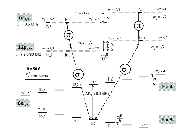
In this section, we suggest a physical implementation of our scheme with ensembles of Cs atoms, placed in linear cavities. Fig. 2 presents a possible choice for the internal states used in our protocol. The reservoir state and the subnode states correspond to different hyperfine components of the ground level
They are coupled to the Rydberg states , with , via the intermediate states and . Note that for the intermediate and Rydberg levels, the hyperfine structure may be neglected, which legitimates the use of the decoupled basis. We assume the availability of light sources and cavities at the wavelengths of the required transitions – i.e. nm and m for the and transitions, respectively 111If the transition is driven via the state with a classical field at nm, the quantum field at the upper transition is at m which conveniently matches telecommunication fibers.. Selection rules show that almost all the transitions necessary to our scheme are allowed and that, in particular, the transitions have different polarizations, that is and , as required (Note that, by setting the quantization axis, i.e. the direction of the applied magnetic field, along the axis of the linear cavity, one highly supresses modes with polarization). Only the direct coupling is not permitted. To overcome this difficulty, we suggest to resort to intermediate states. To be more explicit, to apply a unitary transformation in the subspace we propose to first transfer the population from to , then to run the desired transformation between and – which are indeed coupled, and finally transfer the population back from to . The same trick can be used to emulate a coupling between and : one first transfers the population from to then to then to ; one then applies the desired transformation between and before transferring the population back from to along the same path as in the first step.
Moreover, as indicated on Fig. 2, a magnetic field is applied to lift the degeneracies of the different levels. The specific choice we made, that is G, results in splittings of , for the hyperfine components of the ground level and the excited states , respectively. These splittings assure that the different transitions required by our protocol are selectively addressable, provided that the relevant effective two-photon coupling constant is smaller than MHz and respects the finite lifetime of the Rydberg level; moreover, the detunings from the intermediate states must be chosen larger than kHz, being the lifetime of the level . Typical values of and fulfill the previous requirements, and can be achieved for both “classical-classical” and “quantum-classical” paths in a sample of a few hundreds of atoms with MHz and MHz. Note that the size of the samples should also be small enough so as to remain in the full blockade regime. As shown in BMS07 , a cloud of of a few hundreds of atoms, exhibit Rydberg dipole-dipole interactions of at least , which is indeed much larger than and therefore efficiently forbids multiple Rydberg excitations. Finally, all the two-photon processes required in our protocol, including gates on the quantum register, can be performed on the timescale. Finally, note that the spontaneous emission from the does not constitute a problem when performing unitaries in the subspace through actually populating the state . Indeed, in this case, we must only fulfill the condition MHz to ensure that no unwanted transition such as take place. The frequencies of all the required manipulations – transfers and unitaries , can therefore be taken as large as MHz, while the decay rate of the level is only kHz : the whole unitary process can therefore be run before the decay of the level plays any role.
V Discussion
We now summarize the main differences between our scheme and the most recent works on the subject ZMHZ10 ; HHHLS10 . As noted in ZMHZ10 ; HHHLS10 , the use of Rydberg blocked ensembles allows one to perform entanglement swapping via deterministic manipulations and not through probabilistic photonic detections. The main originality of our proposal is that we also completely got rid of photonic detections during the linking procedure. Indeed, here, photons are simply transmitted from one site and reabsorbed by its neighbor in an efficient and faithful way. The heralded linking is performed only via deterministic ensemble manipulations and ion detections, whose efficiency can be made very close to one. In that respect, our scheme is more of a relay type, as defined in SSRG09 . It is also important to note that, contrary to ZMHZ10 , we do not need different ensembles for encoding what we called “subnodes” in the present work, but use the multilevel structure of the atomic spectrum to store three subnodes in the same ensemble. It therefore means that we do not rely on Rydberg blockade between two ensembles, a rather challenging task. We also note that another proposal for a quantum repeater based on atomic ensembles was put forward in BJG10 . There, however, the authors did not rely on Rydberg blockade phenomenon but rather on fluoresecence detection of excitations stored in the atoms after low intensity laser excitation and Raman scattering.
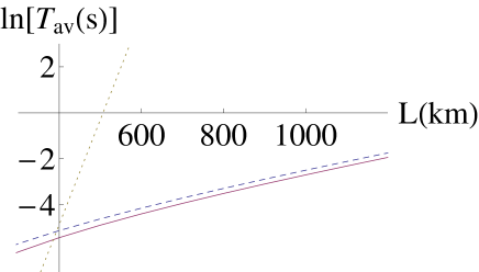
Finally it is worth comparing the total average time needed by our protocol to that required by other schemes, as a figure of merit. Fig. 3 displays the logarithm of the average time necessary for entangling two remote nodes by the direct exchange of a photon – a generous repetition rate of GHz for the photon source was assumed, by the protocol described in ZMHZ10 ; HHHLS10 , and by our protocol as functions of the distance between the two nodes to entangle, for a fixed number of nodes. As in ZMHZ10 ; HHHLS10 , a photodetection efficiency of and a retrieval efficiency of (in our cavity model, this retrieval efficiency was taken equal to one) were assumed. It appears that our protocol is quicker, though asymptotically equivalent for , which is explained by our assumption of the ion detection efficiency exceeding that of photons.
VI Conclusion
In this paper we proposed a quantum repeater scenario based on Rydberg blocked ensembles placed in cavities which are linked by optical fibers. Entanglement generation between two neighboring nodes is performed in a heralded way by the transmission of a photon whose polarization is entangled with the state of the first atomic ensemble, followed by its absorption by the neighboring atomic ensemble. Photon losses and spontaneous emission from the Rydberg level can be detected thanks to an error-syndrome measurement involving ensemble laser manipulations, ionizing pulses and (very efficient) ion detections. An implementation with Cs atoms was suggested and analyzed.
Contrary to protocols previously proposed, the scheme presented here does not make use of any (inefficient) photodetection: this potentially allows for a speedup in the entanglement generation, as confirmed by numerical simulations. Finally main error sources were analyzed. Future work should be devoted to a closer investigation of the practical feasibility of our scheme with real cavities and fibers.
Acknowledgements.
E. B. thanks M. Raoult, Jean-Louis Le Gouet and F. Prats for fruitful discussions.Appendix A Derivation of the expression of the average number of steps in entanglement generation
As described in Sec. III, the entanglement generation procedure is performed in two steps. During each of these steps, subnodes are entangled by pairs. A pair of subnodes is correctly entangled with the probability .
Let us first compute the probability that pairs are correctly entangled within exactly repetitions. This means that, within the first steps, at least one pair is not entangled. Considering all the possible cases, one establishes the following recurrence formula
and, noting that one gets
| (3) | |||||
Setting , one derives from Eq. (3) the relation whence and, since , . One finally deduces the expression for from
The average number of repetitions one needs to entangle the K pairs is simply given by .
Since the entanglement of the two groups of pairs of subnodes and is performed independently and successively, the total average number of repetitions required is simply represented on Fig. 4, or, more explicitly
| (4) | |||||
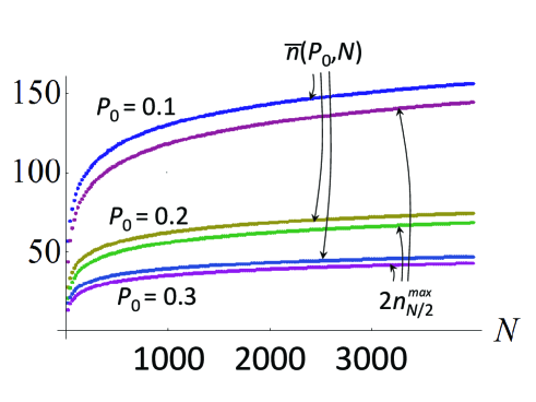
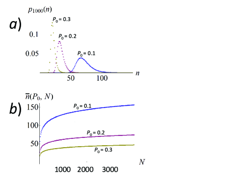
Let us now derive a simple lower bound for . We shall first note that where ; for , one thus has and therefore one can calculate the approximate position of the maximum of by deriving . Doing so, one obtains a maximum for at . As can be seen on Fig. 4, the distribution is not symmetric around its maximum : the position of its peak therefore cannot, strictly speaking, be identified with . It, however, gives a good order of magnitude, , as can be checked on Fig. 5. In particular, the expression of gives a good indication on how scales with the physical parameters.
References
- (1) C. H. Bennett et al., Phys. Rev. Lett. 70, 1895 (1993).
- (2) C. H. Bennett et al., Phys. Rev. A 54, 3824 (1996).
- (3) H. J. Briegel, W. Dï¿œr, J. I. Cirac and P. Zoller, Phys. Rev. Lett. 81, 5932 (1998).
- (4) L. M. Duan, M. D. Lukin, J. I. Cirac and P. Zoller, Nature 414, 413 (2001).
- (5) A. Kuzmich, W. P. Bowen, A. D. Boozer, A. Boca, C. W. Chou, L.-M. Duan, and H. J. Kimble, Nature 423, 731 (2003).
- (6) D. Comparat and P. Pillet, J. Opt. Soc. Am. B 27, A208 (2010).
- (7) E. Urban, T. A. Johnson, T. Henage, L. Isenhover, D. D. Yavuz, T. G. Walker, and M. Saffman, Nature Physics 5, 110 (2009).
- (8) T. Vogt, M. Viteau, J. Zhao, A. Chotia, D. Comparat, and P. Pillet, Phys. Rev. Lett. 97, 083003 (2006).
- (9) D. Jaksch, J. I. Cirac, P. Zoller, S. L. Rolston, R. Cᅵtᅵ, and M. D. Lukin, Phys. Rev. Lett. 85, 2208 (2000).
- (10) M. Saffman, T. G. Walker, and K. Mï¿œlmer, Rev. Mod. Phys. 82, 2313 (2010).
- (11) E. Brion, A. S. Mouritzen, and K. Mï¿œlmer, Phys. Rev. A 76, 022334 (2007).
- (12) E. Brion, L. H. Pedersen, K. Mï¿œlmer, S. Chutia, and M. Saffman, Phys. Rev. A 75, 032328 (2007).
- (13) E. Brion, L. H. Pedersen and K. Mï¿œlmer, J. Phys. B: At. Mol. Opt. Phys. 40, S159–S166 (2007).
- (14) M. D. Lukin, M. Fleischhauer, R. Cote, L. M. Duan, D. Jaksch, J. I. Cirac, and P. Zoller, Phys. Rev. Lett. 87, 037901 (2001).
- (15) E. Brion, K. Mï¿œlmer, and M. Saffman, Phys. Rev. Lett. 99, 260501 (2007).
- (16) E. Brion, L. H. Pedersen, M. Saffman, and K. Mï¿œlmer, Phys. Rev. Lett. 100, 110506 (2008).
- (17) B. Zhao, M. Mï¿œller, K. Hammerer, and P. Zoller, Phys. Rev. A 81, 052329 (2010).
- (18) Y. Han, B. He, K. Heshami, C.-Z. Li, and C. Simon, Phys. Rev. A 81, 052311 (2010).
- (19) E. Brion, L. H. Pedersen and K. Mï¿œlmer, J. Phys. A: Math. Theor. 40, 1033 (2007).
- (20) C. Guerlin, E. Brion, T. Esslinger, and Klaus Mï¿œlmer, Phys. Rev. A 82, 053832 (2010).
- (21) T. Pellizzari, Phys. Rev. Lett. 79, 5242–5245 (1997).
- (22) N. Sangouard, C. Simon, H. de Riedmatten, and N. Gisin, Rev. Mod. Phys 83, 33 (2011).
- (23) J. B. Brask, L. Jiang, A. V. Gorshkov, V. Vuletic, A. S. Sï¿œrensen and M. D. Lukin, Phys. Rev. A 81, 020303 (2010).