Abstract

We apply analytic perturbation theory to the QCD analysis of the $xF_{3}$ structure function data of the CCFR collaboration. We use different approaches for the leading order $Q^{2}$ evolution of the $xF_{3}$ structure function and compare the extracted values of the parameter $\Lambda$ and the shape of the higher twist contribution. Our consideration is based on the Jacobi polynomial expansion method of the unpolarized structure function. The analysis shows that the analytic approach provides reasonable results in the leading order QCD analysis.

1 Introduction

The data on the $xF_{3}$ structure function [1] provide a possibility for a precise test of the perturbative QCD predictions for the $Q^{2}$ evolution of this structure function. The analysis of $xF_{3}$ data is simplified because one does not need to parameterize gluon and see quark contributions and can parameterize the shape of the $xF_{3}$ structure function itself at some value $Q^{2}_{0}$. For the kinematics region of these data $Q^{2}$ $\geq 1.3$ GeV² the higher twist (HT) contribution to the structure function should be taken into account. This allows us to study from the above-mentioned data both the perturbative part and the HT correction related to each other. Here, we will focus our attention on the interplay of the different approaches to the strong coupling $Q^{2}$-behavior and the $x$-dependence of the HT contribution.

In our investigation we apply the analytic approach in QCD proposed by Shirkov and Solovtsov [2], the so-called analytic perturbation theory (APT) (see also Refs. [3, 4]). This method takes into account the basic principles of local quantum field theory which in the simplest cases is reflected in the form of $Q^{2}$-analyticity of the Käll$\acute{{\rm e}}$n–Lehmann type. The key point of APT constructions—the analytic properties of some functions (the two-point correlator of the quark currents, the moments of the structure functions and so on). An overview of the analytic approach to QCD can be found in Ref. [5]. In the framework of the APT, in contrast to the infrared behavior of the perturbative (PT) running coupling, the analytic coupling has no unphysical singularities. At low $Q^{2}$ scales, instead of rapidly changing $Q^{2}$ evolution as occurs in the PT case, the APT approach leads to slowly changing functions (see, e.g., Refs. [6, 7]). In the asymptotic region of large $Q^{2}$ the APT and the PT approaches coincide. It should be noted that the moments of the structure functions should be analytic functions in the complex $Q^{2}$ plane with a cut along the negative real axis (see Ref. [8] for more details), the ordinary PT description violates analytic properties due to the unphysical singularities of PT coupling. On the other hand, the APT supports these analytic properties. For fullness, in our analysis, we consider also the recent variant of the model for the freezing-like behaviour coupling – “massive analytic perturbative QCD” (MPT) [9] (see Ref. [10, 11] for a discussion).

In Refs. [12, 13] further development of the APT method was made – the generalization to the fractional powers of the running coupling which is called the Fractional Analytic Perturbation Theory (FAPT) (see Ref. [14] as review). The FAPT technique was applied to analyze the $F_{2}$ structure function behavior at small $x$-values [11, 15], to analyze the low energy data on nucleon spin sum rules $\Gamma_{1}^{p,n}(Q^{2})$ [16], to calculate binding energies and masses of quarkonia [17]. Here, we continue applications of the APT/FAPT approach executing the data on the $xF_{3}$ structure function and investigating how the analytic approach works in this case by comparison with the standard PT analysis.

2 The Method of the QCD analysis

In our analysis, we will follow the well-known approach based on the Jacobi polynomial expansion of structure functions. This method of solution of the DGLAP equation was proposed in Ref. [18] and developed for both unpolarized [19] and polarized cases [20]. The main formula of this method allows an approximate reconstruction of the structure function through a finite number of Mellin moments of the structure function

$$xF_{3}^{N_{max}}(x,Q^{2})=\frac{h(x)}{Q^{2}}+x^{\alpha}(1-x)^{\beta}\sum_{n=0}^{N_{max}}\Theta_{n}^{\alpha,\beta}(x)\sum_{j=0}^{n}c_{j}^{(n)}{(\alpha,\beta)}M_{j+2}\left(Q^{2}\right).$$ (1)

The $Q^{2}$-evolution of the moments $M_{N}(Q^{2})$ in the leading order (LO) perturbative QCD is defined by

$$M^{QCD}_{N}(Q^{2})=\left[\frac{\alpha_{s}\left(Q^{2}\right)}{\alpha_{s}\left(Q_{0}^{2}\right)}\right]^{{\frac{\gamma^{(0),N}}{2\beta_{0}}}}M_{N}^{QCD}(Q^{2}_{0}),~{}~{}~{}N=2,~{}3,...\,.$$ (2)

Here  $\alpha_{s}(Q^{2})$  is the QCD running coupling,  $\gamma^{(0),N}$  are the nonsinglet leading order anomalous dimensions, $\beta_{0}=11-2n_{f}/3$ is the first coefficient of the renormalization group $\beta$-function, and $n_{f}$ denotes the number of active flavors.

Unknown coefficients $M_{N}^{QCD}(Q^{2}_{0})$ in Eq. (2) could be parameterized as the Mellin moments of some function:

$$M_{3}^{QCD}(N,Q^{2}_{0})=\int_{0}^{1}dx{x^{N-2}}Ax^{a}(1-x)^{b}(1+\gamma~{}x),~{}~{}N=2,3,...~{}~{}.$$ (3)

The shape of the function $h(x)$ as well as parameters A, $a$, $b$, $\gamma$, and $\Lambda_{\rm{QCD}}$ are found by fitting the experimental data to the $xF_{3}(x,Q^{2})$ structure function [1]. The detailed description of the fitting procedure could be found in Ref. [21]. The term $h(x)/Q^{2}$ is considered as pure phenomenological. The target mass corrections are taken into account to the order $o(M^{4}_{nucl}/Q^{4})$.

3 Analytic approach in QCD

The APT method gives the possibility of combining the renormalization group resummation with correct analytic properties in $Q^{2}$-variable for some physical quantities and provides also a well-defined algorithm for calculating higher-loop corrections [4]. As the difference between the APT and PT running couplings becomes significant at low $Q^{2}$-scales (see, e.g., Fig. 1 in Ref. [6]) this stimulates applications of the analytic approach to a new analysis [5], especially after the generalization of the APT to the fractional powers of the running coupling (see Refs. [14, 22, 23] for further details).

In the framework of the analytic approach the following modification in the standard PT expression (2) for the $Q^{2}$-evolution of the moments $M_{N}(Q^{2})$ is required: $\left[\alpha_{\rm PT}(Q^{2})\right]^{\nu}\Rightarrow$ ${\cal{A}}_{\nu}(Q^{2})$. It transforms Eq. (2) as follows:

$${\cal{M}}^{QCD}_{N}(Q^{2})=\frac{{\cal{A}}_{\nu}(Q^{2})}{{\cal{A}}_{\nu}(Q_{0}^{2})}\,{\cal{M}}_{N}^{QCD}(Q^{2}_{0})~{},~{}~{}{\nu}\equiv{\frac{\gamma^{(0),N}}{2\beta_{0}}}\,,$$ (4)

where the analytic function ${\cal{A}}_{\nu}$ is derived from the spectral representation and corresponds to the discontinuity of the $\nu$-th power of the PT running coupling

$${\cal{A}}_{\nu}(Q^{2})\,=\,\frac{1}{\pi}\,\int_{0}^{\infty}\,\frac{d\sigma}{\sigma\,+\,Q^{2}}\,{\rm Im}\;\left\{{\alpha}_{\rm PT}^{\nu}(-\sigma-{\rm i}\varepsilon)\right\}\,.$$ (5)

Note that the function ${\cal{A}}_{1}(Q^{2})$ defines the APT running coupling: ${\alpha}_{\rm APT}(Q^{2})$ $\equiv{\cal{A}}_{1}(Q^{2})\,$. The mathematical tool for numerical calculations of ${\cal{A}}_{\nu}$ for any $\nu>0\,$ up to four-loop order in the perturbative running coupling is given in Ref. [25].

The ‘normalized’ analytic function $\bar{\cal{A}}_{\nu}=\beta_{0}{\cal{A}}_{\nu}/(4\pi)$ in the leading order (LO) has rather a simple form (see, e.g., [14]) and can be writhen as

$$\bar{\cal{A}}_{\nu}^{LO}(Q^{2})=\left[\bar{a}^{LO}_{\rm PT}(Q^{2})\right]^{\nu}\,-\,\frac{{\rm{Li}_{\delta}}(t)}{\Gamma(\nu)}\,,$$ (6)

$$~{}{\rm{Li}}_{\delta}(t)=\sum_{k=1}^{\infty}\frac{t^{k}}{k^{\delta}},~{}~{}t=\frac{\Lambda^{2}}{Q^{2}},~{}~{}~{}\delta=1-\nu,~{}$$

where the ‘normalized’ PT running coupling $\bar{a}^{LO}_{\rm PT}(Q^{2})=\beta_{0}{{\alpha}_{\rm PT}^{LO}(Q^{2})}/(4\pi)=1/\left[\ln(Q^{2}/\Lambda^{2})\right]\,$ and Li_δ is the polylogarithm function. For ${\nu=1}$ expression (6) leads to the well-known one-loop APT result [2]

$$\alpha_{\rm APT}^{LO}(Q^{2})={\alpha}_{\rm{PT}}^{LO}(Q^{2})+\frac{4\pi}{\beta_{0}}\,\frac{\Lambda^{2}}{\Lambda^{2}-Q^{2}}\,.$$ (7)

One could see that at large $Q^{2}$ the second term in the r.h.s. of expression (7) is negative. It was confirmed qualitatively in the phenomenological analysis of the $xF_{3}$ data in Ref. [26].

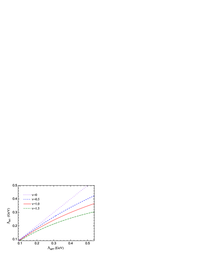
Figure 1: The behavior of the parameter $\Lambda_{{\rm PT}}$ vs. $\Lambda_{{\rm APT}}$ in LO for different values of $\,\nu\,$ at $Q_{0}^{2}=3$ GeV².

It should be stressed that values of the QCD scale parameter $\Lambda$ are different in the PT and APT approaches. In order to illustrate this, in Fig. 1, we present the behavior following from the condition $\left[\alpha_{\rm PT}^{LO}(Q_{0}^{2},\Lambda_{{\rm PT}})\right]^{\nu}={\cal{A}}_{\nu}^{LO}(Q_{0}^{2},\Lambda_{{\rm APT}})$ of the parameter $\Lambda_{{\rm PT}}$ vs. $\Lambda_{{\rm APT}}$ for different values of $\,\nu\,$.

In short, one-loop modification of the QCD coupling within the MPT approach which will be considered further corresponds to the replacement of the logarithm in the ${\alpha}_{\rm{PT}}^{LO}(Q^{2})$ to the “long logarithm” with the “effective gluonic mass” $m_{gl}$: $\ln(Q^{2}/\Lambda^{2})\Rightarrow\ln[(Q^{2}+m_{gl}^{2})/\Lambda^{2}]$ (see, Refs. [9, 28]).

4 Numerical analysis of experimental data

The results of the LO QCD fit in different approaches are presented in Table 1 and Figs. 2–5. Both cases $h(x)$– free and $h(x)=0$ are considered for $Q^{2}_{0}=3$ GeV², $Q^{2}>1.3$ GeV², $n_{f}=4$, and $N_{Max}=12$. In order to reconstruct the $x$-shape of the HT contribution, we have parameterized $h(x)$ in the number of points $x_{i}$ = 0.015, 0.045, 0.080, 0.125, 0.175, 0.225, 0.275, 0.35, 0.45, 0.55, 0.65 - one per $x$-bin. The values of A, $a$, $b$, $\gamma$, $x_{i}$ and $\Lambda$ are considered as free parameters.

Table 1: The results for the QCD leading order fit (with TMC) of $xF_{3}$ data [1] ($Q^{2}_{0}=3$ GeV², $Q^{2}>1$ GeV², $n_{f}=4$, and $N_{Max}=12$).

	$h(x)=0$		$h(x)$–free
Approach	$\Lambda$ (MeV)	$\chi^{2}_{d.f.}$	$\Lambda$ (MeV)	$\chi^{2}_{d.f.}$
PT	$291\pm 36$	$1.35$	$363\pm 170$	$0.984$
APT	$275\pm 39$	$1.42$	$350\pm 145$	$0.980$
MPT	$299\pm 38$	$1.35$	$351\pm 128$	$0.985$
“naive” analyt.	$417\pm 83$	$1.34$	$412\pm 240$	$0.980$

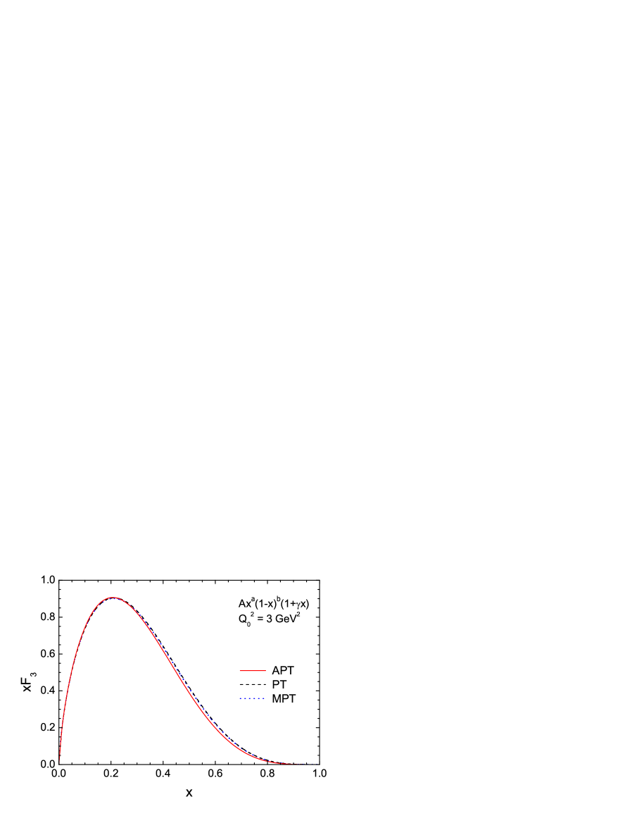
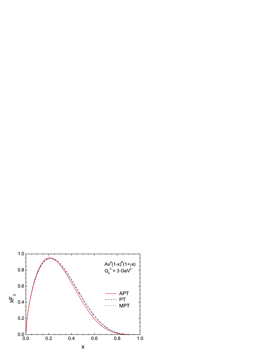
Figure 2: Comparison of parametrizations of $xF_{3}$ in the PT, APT and MPT approaches for $h(x)=0$.

      Figure 3: Comparison of parametrizations of $xF_{3}$ in the PT, APT and MPT approaches for $h(x)\neq 0$.

As can be seen from Table 1, the values of parameter the $\Lambda$ for the case $h(x)=0$ are smaller in comparison with the case of nonzero HT contribution. The difference of the $\Lambda$ values for APT and PT are smaller in the analysis with the HT contribution: $(\Lambda_{{\rm PT}}-\Lambda_{{\rm APT}})_{h(x)=0}>(\Lambda_{{\rm PT}}-\Lambda_{{\rm APT}})_{h(x)\neq 0}$. The LO $h(x)=0$ results for $\Lambda$ values are consistent within errors. If one adds the HT contribution, the values of parameter the $\Lambda$ and their errors are higher than $h(x)=0$ case.

For illustrative purposes we present in the last line of Table 1 the result corresponding to the use in the analysis of “naive analytization” when the ordinary perturbative coupling is replaced by the analytic coupling: ${\alpha}_{\rm{PT}}(Q^{2})\to\alpha_{\rm APT}(Q^{2})$ (see Ref. [12] and references therein).

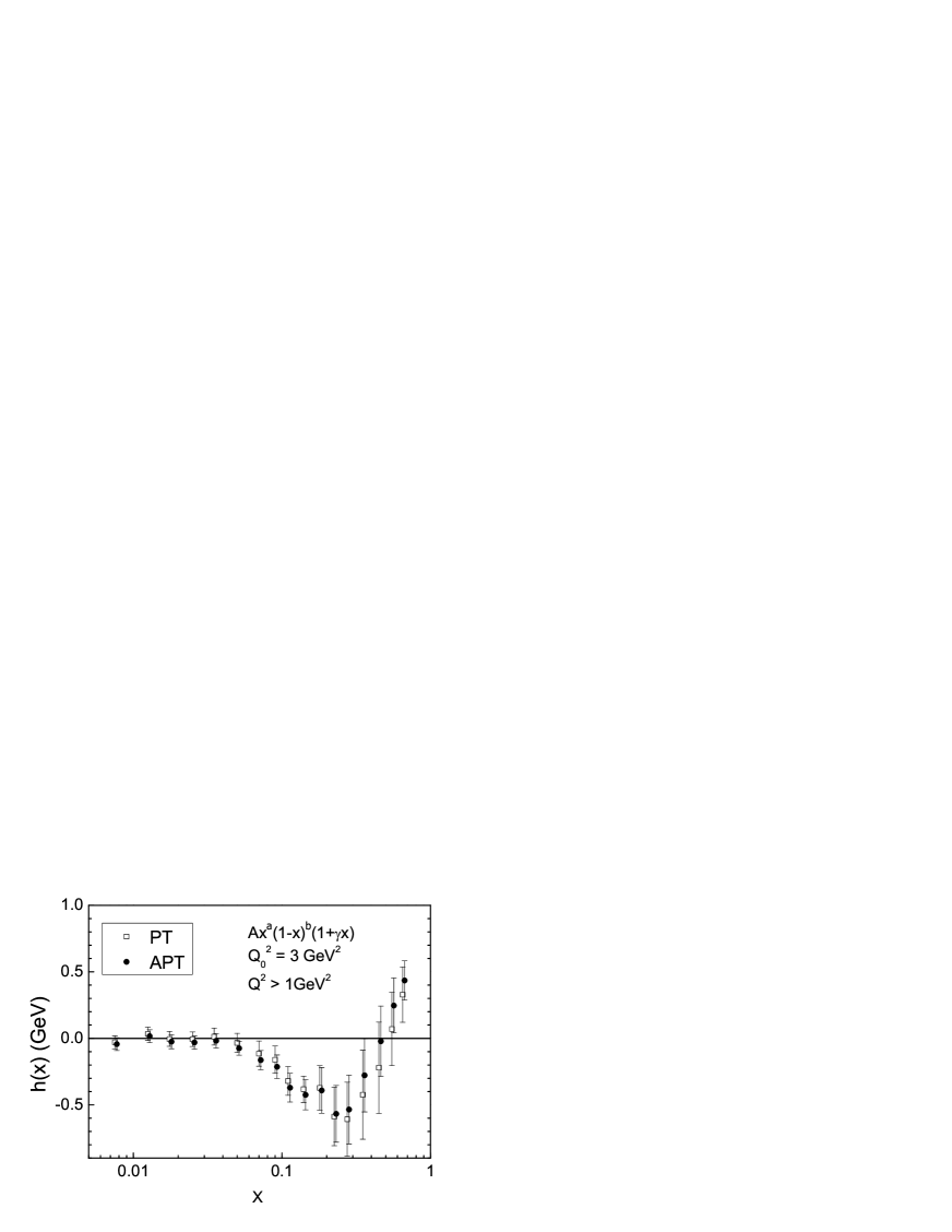
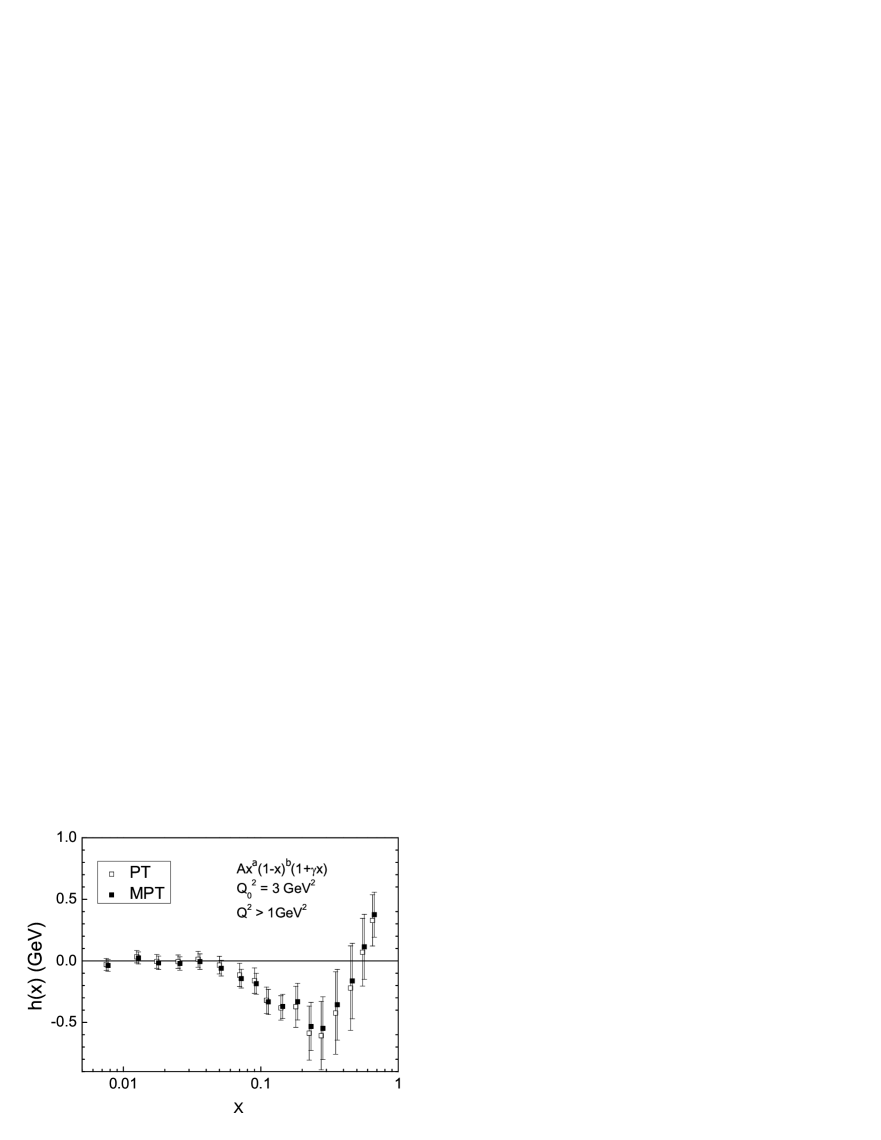
Figure 4: Higher twist contribution resulting from the LO QCD analysis of $xF_{3}$ data [1] for the PT and APT approaches.

      Figure 5: Higher twist contribution resulting from the LO QCD analysis of $xF_{3}$ data [1] for the PT and MPT approaches.

Figures 2–3 show the $xF_{3}$-shape obtained in the APT, PT and MPT approaches without taking into account the HT term (Fig. 2) and with the HT (Fig. 3). In both cases, the result for the APT approach is slightly higher than for the PT and MPT ones for small $x$ and less for large $x$.

Figures 4–5 demonstrate the shape of the HT contribution. From Fig. 4 one can see that for $x>0.3$ we obtained $h^{APT}(x)>h^{PT}(x)$. This inequality is in qualitative agreement with the result obtained in LO for the shape of the HT contribution for the non-singlet part of the $F_{2}$ structure function (see Table 3 in Ref. [11]). The opposite inequality is obtained for small values $x<0.2\,$: $h^{APT}(x)<h^{PT}(x)$. Figure 5 shows that the central values of $h^{PT}(x)$ and $h^{MPT}(x)$ are very close to each other.

5 Conclusion

We performed the QCD analysis of the $xF_{3}$ structure function data based on the analytic approach. It should be noted that the wide kinematic region experimental points gave us the possibility to analyze HT contributions of both small and relatively large $x$ and to compare the APT and MPT results to the PT one. We have found that in the examined region $Q^{2}>1$ GeV² the values of $\Lambda$ obtained in the PT, APT and MPT approaches are close to each other, while the “naive analytization” approach leads to a rather large $\Lambda$ value. The shape of the HT contributions is in quantitative agreement with the results of the previous analysis of the $xF_{3}$ structure function data. We made the first step – LO analysis which showed that the analytic approach gives reasonable results. It is important to extend the analysis to higher orders and apply it to the structure function data in the low $Q^{2}$ region.

Acknowledgments

It is a pleasure for the authors to thank V.L. Khandramai, S.V. Mikhailov, and O.V. Teryaev for interest in this work and helpful discussions. This work was partly supported by the RFBR grants 11-01-00182 and 13-02-01005 and the BelRFFR- JINR grant F12D-002.

References

- [1] CCFR-NuTeV Collab., W.G. Seligman et al., Phys. Rev. Lett. 79, 1213 (1997).
-
[2]
D.V. Shirkov, I.L. Solovtsov,
JINR Rap. Comm. 1996. No. 2[76]-96, 5 (1996);
Phys. Rev. Lett. 79, 1209 (1997). - [3] K.A. Milton, I.L. Solovtsov, Phys. Rev. D 55, 5295 (1997).
- [4] I.L. Solovtsov, D.V. Shirkov, Theor. Math. Phys. 120, 1220 (1999).
- [5] D.V. Shirkov, I.L. Solovtsov, Theor. Math. Phys. 150, 132 (2007).
- [6] K.A. Milton, I.L. Solovtsov, O.P. Solovtsova, Phys. Rev. D 60, 016001 (2001).
- [7] V.L. Khandramai, R.S. Pasechnik, D.V. Shirkov, O.P. Solovtsova, O.V. Teryaev, Phys. Lett. B 706, 340 (2012).
- [8] I.L. Solovtsov, Part. Nucl. Lett. 4[101], 10 (2000).
- [9] D.V. Shirkov, Phys. Part. Nucl. Lett. 10, 186 (2013), arXiv:1208.2103 [hep-ph].
- [10] F.J. Yndurain, The Theory of Quark and Gluon Interactions, Springer, 2006, 476 pp., Chapt. 4.
- [11] A.V. Kotikov, V.G. Krivokhizhin, B.G. Shaikhatdenov, Phys. Atom. Nucl. 75, 507 (2012).
-
[12]
A.P. Bakulev, S.V. Mikhailov, N.G. Stefanis, Phys. Rev. D
72, 074014 (2005);
Erratum: ibid. D 72, 119908(E) (2005). -
[13]
A.P. Bakulev, S.V. Mikhailov, N.G. Stefanis, Phys. Rev. D
75, 056005 (2007);
Erratum: ibid. D 77, 079901(E) (2008). - [14] A.P. Bakulev, Phys. Part. Nucl. 40, 715 (2009).
- [15] G. Cvetic, A.Y. Illarionov, B.A. Kniehl, A.V. Kotikov, Phys. Lett. B 679, 350 (2009).
- [16] R.S. Pasechnik, D.V. Shirkov, O.V. Teryaev, O.P. Solovtsova, V.L. Khandramai, Phys. Rev. D 81, 016010 (2010).
- [17] C. Ayala, G. Cvetic, Phys. Rev. D 87, 054008 (2013).
- [18] G. Parisi, N. Sourlas, Nucl. Phys. B 151, 421 (1979).
-
[19]
I.S. Barker, C.B. Langensiepen, G. Shaw, Nucl. Phys.
B 186, 61 (1981);
V.G. Krivokhizhin et al., Z. Phys. C 36, 51 (1987), Z. Phys. C 48, 347 (1990);
A.V. Kotikov, G. Parente, J. Sanchez-Guillen, Z. Phys. C 58, 465 (1993);
A.L. Kataev, A.V. Sidorov, Phys. Lett. B 331, 179 (1994);
A.L. Kataev et al., Phys. Lett. B 388, 179 (1996);
A.V. Sidorov, Phys. Lett. B 389, 379 (1996); JINR Rapid Comm. 80 (1996) 11, [hep-ph/9609345]. -
[20]
E. Leader, A.V. Sidorov, D.B. Stamenov, Int. J. Mod. Phys. A 13, 5573 (1998);
Phys. Rev. D 58 (1998) 114028;
C. Bourrely et al., Phys. Lett. B 442, 479 (1998). - [21] A.L. Kataev et al., Phys. Lett. B 417, 374 (1998).
- [22] G. Cvetic, A.V. Kotikov, J. Phys. G G39, 065005 (2012).
- [23] N.G. Stefanis, Acta Phys. Polon. Supp. 6, 71 (2013).
- [24] C. Ayala, S.V. Mikhailov, in preparation.
- [25] A.P. Bakulev, V.L. Khandramai, Comput. Phys. Commun. 184, 183 (2013).
- [26] A.V. Sidorov, Nuovo Cim. A 112, 1527 (1999).
- [27] E.G.S. Luna, A.A. Natale, A.L. dos Santos, Phys. Lett. B 698, 52 (2011).
- [28] G. Cvetic, arXiv:1309.1696 [hep-ph].