Pre-merger localization of eccentric compact binary coalescences with second-generation gravitational-wave detector networks
Abstract
We study the possibility of pre-merger localization of eccentric compact binary coalescences by second-generation gravitational-wave detector networks. Gravitational waves from eccentric binaries can be regarded as a sequence of pulses, which are composed of various higher harmonic modes than ones with twice the orbital frequency. The higher harmonic modes from a very early inspiral phase will not only contribute to the signal-to-noise ratio, but also allow us to localize the gravitational-wave source before the merger sets in. This is due to the fact that high-frequency gravitational waves are essential for the source localization via triangulation by ground-based detector networks. We found that the single-detector signal-to-noise ratio exceeds 5 at 10 min before the merger for a 1.4– eccentric binary neutron stars at 100 Mpc in optimal cases, and it can be localized up to 10 deg2 at half a minute before the merger by a four-detector network. We will even be able to achieve 10 deg2 at 10 min before the merger for a face-on eccentric compact binary by a five-detector network.
keywords:
gravitational waves — methods: data analysis — binaries: close — stars: neutron1 introduction
Gravitational waves from compact binary coalescences are expected to be detected in the coming decade by second-generation gravitational-wave detectors like Advanced LIGO, Advanced Virgo, and KAGRA (Harry & LIGO Scientific Collaboration, 2010; Accadia et al., 2011; Somiya, 2012). Gravitational waves will give us a way to infer masses and spins of binary components, and also equations of state for supranuclear-density matter if the binary involves a neutron star. In addition to these intrinsic parameters, extrinsic parameters such as the luminosity distance and sky position of the binary can also be studied by gravitational-wave observation. Once we localize a compact binary coalescence in the sky to the extent that the host galaxy is determined, the luminosity distance will be known as a function of the cosmological redshift so that a new distance ladder may be constructed (Schutz, 1986). Electromagnetic counterparts of compact binary coalescences are also important at this stage (Metzger & Berger, 2012; Piran et al., 2013), because seeing them is more advantageous for accurate localization than hearing gravitational waves.
One ambitious goal of gravitational-wave astronomy is to sound a merger alert before the merger sets in. The benefit of realtime electromagnetic observation of the compact binary merger will be immeasurable. Nearly simultaneous detection of gravitational and electromagnetic waves will give us an opportunity to investigate the propagation speed of gravitational waves as SN 1987A did for neutrinos (Bionta et al., 1987; Hirata et al., 1987). Realtime observation of the merger is also useful to understand electromagnetic radiation mechanisms. If short-hard gamma-ray bursts are driven by compact binary coalescences (see Nakar 2007; Berger 2013 and references therein for reviews), we will be able to detect prompt emission from the beginning in various wavelengths for face-on compact binaries. Recent possible ‘kilonova’ detection supports this binary merger scenario of the short-hard gamma-ray burst (Berger et al., 2013; Hotokezaka et al., 2013; Tanvir et al., 2013), and we can reasonably expect simultaneous detection with gravitational waves. Still, direct connection between the short-hard gamma-ray bursts and gravitational waves is essential for the robust confirmation of the scenario. The onset of afterglow will be observed following the prompt emission. Extended emission observed in the afterglow is one of the most mysterious feature of the short-hard gamma-ray bursts (e.g. Nakamura et al. 2013; Veres & Mészáros 2013), and detailed characteristics including its opening angle will be investigated if a merger alert could be sounded. Other electromagnetic events involving ultrarelativistic outflows, such as a proposed shock breakout emission from binary neutron star mergers (Kyutoku et al., 2014), are also easier to detect with realtime observation.
Besides the signal-to-noise ratio (SNR), localization of the gravitational-wave source up to moderate accuracy is necessary for successful follow-up detection of electromagnetic counterparts (Nissanke et al., 2013; LIGO Scientific Collaboration and Virgo Collaboration, 2013), and thus pre-merger localization should be regarded as a prerequisite for generating merger alerts. Pointing only known galaxies using available catalogues will help to detect electromagnetic counterparts particularly in the early era of gravitational-wave astronomy (Nuttall & Sutton, 2010). Still, assuming the number density of galaxies to be 0.01 Mpc-3, 8 galaxies per deg2 will be found if we are going to observe out to 200 Mpc. Thus, accurate localization is eagerly desired irrespective of our follow-up strategy.
Detection and localization of circular binaries on the celestial sphere prior to the merger are challenging tasks (Abadie et al., 2012; Cannon et al., 2012; Evans et al., 2012), whereas such binaries will be the most frequent sources and are extensively studied. The reason for this is that a circular binary has the largest periapsis distance for a fixed value of the semimajor axis, and the luminosity averaged over an orbit is the lowest among possible configurations. Furthermore, gravitational-wave frequency is only twice the orbital frequency within the quadrupole approximation. The localization of gravitational-wave sources is primarily based on triangulation via the timing difference between detectors (Fairhurst, 2011). Typical separations of ground-based detectors determine typical timing differences ms, and thus accurate localization requires gravitational waves with frequency higher than Hz. But, the gravitational-wave frequency from 1.4– binary neutron stars in a circular orbit does not reach 10 Hz until 1000 s before the merger, and reaches 100 Hz only at 2 s before the merger. As a result, the area of the 90 per cent localization confidence will be larger than 100 deg2 even 1 s before the merger for typical events (Cannon et al., 2012). Moreover, the SNR does not substantially accumulate until gravitational-wave frequency reaches 100 Hz, because each detector is sensitive around 100 Hz. Taking a few to 10 min of latency associated with trigger and alert generation into account (Cannon et al., 2012), it would be challenging to sound merger alerts with second-generation detector networks even if we could omit human validation processes. Furthermore, practical target-of-opportunity observation will involve overheads of telescopes and satellites as additional latency sources.
The situation could be changed for eccentric compact binary coalescences (e.g. O’Leary et al. (2009)), which emit higher mode gravitational waves even within the quadrupole approximation (Peters & Mathews, 1963). Event rates of eccentric compact binary coalescences are conceivably low, and several authors investigated this possibility. Note that the horizon distance 200 Mpc of a single detector is not changed drastically by the presence of a finite eccentricity unless the binary is formed with an extremely short periapsis distance as we discuss later. Lee et al. (2010) studied the formation of very hard eccentric binaries via tidal-interaction induced captures in globular clusters focusing on nearly direct collisions. They found that the local formation rate of binary neutron stars may be a few tens Gpc-3 yr-1 depending on globular cluster models. Although this rate is motivating for ground-based detectors, East et al. (2013) pointed out that this might be an order-of-magnitude overestimation caused by assuming extremely high retention fraction of neutron stars (see also Tsang 2013). At the same time, East et al. (2013) also pointed out that the cross-section of gravitational-wave induced captures is larger than that of the tidal-interaction ones by an order of magnitude. Indeed, whereas the tidal capture requires the initial periapsis distance to be smaller than – for binary neutron stars with the total mass , where and are the gravitational constant and speed of light, respectively (Lee et al., 2010), the gravitational-wave capture can work up to – irrespective of the binary components (O’Leary et al., 2009). Thus, the merger rate of eccentric binary neutron stars could be 1 yr-1 within the sensitive volume of second-generation gravitational-wave detectors. Here, we would not say that such eccentric compact binary coalescences are frequent enough, because the rate estimation is not settled.111It is suggested that dynamical binary-stellar encounters could be another efficient channel of eccentric compact binary formation (Samsing et al., 2014). It is also suggested that the Kozai mechanism in hierarchical triples could reduce the time to the merger of inner compact binaries by several orders of magnitude, and enhance the merger rate (Antonini & Perets, 2012; Seto, 2013; Antognini et al., 2014). Instead, we consider that they can be possible events and should not be completely neglected in the gravitational-wave data analysis. Note that an eccentric binary formed with a very large periapsis distance essentially circularizes before gravitational waves are detected, where the distribution of is expected to be flat below from the fact that the capture cross-section is proportional to .
In this paper, we explore a possibility of realtime detection and localization of moderately eccentric compact binary coalescences. Here, we use the word ‘moderately eccentric’ to state that the binary is eccentric during a detectable inspiral phase, and circularized to a low value of eccentricity, say , when it reaches the last stable orbit. In such cases, the remnant of the merger and associated electromagnetic counterparts are expected to be more similar to those of circular compact binary coalescences than those of direct collisions. We only focus on equal-mass, 1.4– binary neutron stars in this study, and our result depends only weakly on the total mass and mass ratio once effects of the eccentricity are properly normalized with respect to the chirp mass. We always assume that binary components are treated as non-spinning point particles up to the last stable orbit, while the exact merger is determined by the radius of neutron stars.
The paper is organized as follows. In Section 2, we briefly summarize the orbital evolution of eccentric binaries. Next, in Section 3, our formalism to evaluate the SNR, timing accuracy, and localization accuracy is described. Results are shown in Section 4, and Section 5 is devoted to the summary and discussion. We denote masses of each component by and . The total mass and reduced mass are written by and , respectively. The distance to the binary from the earth (or Solar system barycentre) is written by . The semimajor axis and eccentricity of the binary are denoted by and , respectively.
2 binary evolution
We describe the motion of an eccentric binary with and in Newtonian gravity, and consider gravitational radiation in terms of quadrupole formula. The orbital frequency as the inverse of the period is given by
| (1) |
and gravitational waves are decomposed into harmonic modes with frequency
| (2) |
where (Peters & Mathews, 1963). The luminosity of each harmonic mode averaged over an orbit is given by
| (3) |
where is given by equation 20 of Peters & Mathews (1963). We have
| (4) |
and the total luminosity averaged over an orbit , which governs the orbital evolution, is given in terms of .
Time evolution of an eccentric binary due to radiation reaction is handled following O’Leary et al. (2009) in this study. Specifically, we use the eccentricity, , as the independent variable, and describe all quantities including the time to the merger as functions of . The time evolution of and are derived under the assumption of adiabatic evolution according to Peters (1964), whereas the actual evolution may be more discontinuous due to the pulse-like nature of gravitational waves from a highly eccentric binary. This approximation may require sophistication once we are going to prepare waveform templates, and we do not expect that it changes the story as far as pulse-like gravitational-wave trains are emitted.
The periapsis distance is given by , and we introduce a normalized periapsis distance
| (5) |
for convenience. We further introduce an initial normalized periapsis distance at as . Although realistic binaries should be formed with an eccentricity smaller than unity, we consider the evolution of a binary from as an approximation. This approximation can be relaxed by evolving a binary from a realistic initial value at , but we do not take this step so that the formation process is kept unspecified. The change of quantities such as SNRs associated with setting is negligible due to its proximity to unity if we assume gravitational-wave induced captures (see Fig. 1).
The periapsis distance evolves in time according to (O’Leary et al., 2009)
| (6) |
where
| (7) |
This implies that
| (8) | ||||
| (9) |
The formal time to the merger, at which is achieved, is given by
| (10) |
We use this to denote the time to the merger, whereas we truncate gravitational radiation at a finite eccentricity of the last stable orbit, at which
| (11) |
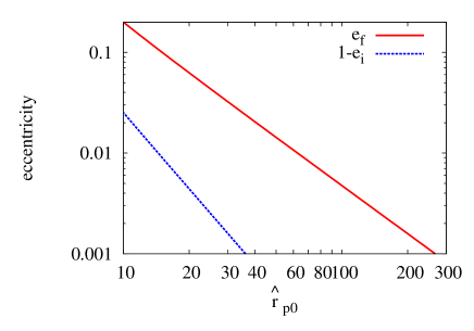
Fig. 1 shows the value of as a function of as well as (deviation from the unity of) the initial eccentricity
| (12) |
for a gravitational-wave induced capture as an example formation process (O’Leary et al., 2009). The eccentricity at the merger, which may correspond roughly to that at the last stable orbit, is less than 0.1 for , and thus we expect that the merger outcome and electromagnetic counterparts are closer to those for circular cases than those for direct collisions. The time to the merger from the initial eccentricity is
| (13) | ||||
| (14) |
and this is approximately twice the orbital period at the formation, which is also proportional to . Here, formation via the gravitational-wave induced capture is assumed and equation (12) is used. The specific values of are half an hour, 3 d, and 3 yr for , 100, and 300, respectively. Since the orbital period, which is proportional to , after periastron passages decreases as in a high-eccentricity regime, more than 10 orbits are always expected as far as the binary is formed with . This may validate the use of the adiabatic approximation, whereas the discontinuous nature of eccentric binary evolution should be considered seriously in practice, especially for binaries formed with small values of .
3 data analysis
We estimate the localization accuracy of a gravitational-wave source adopting the timing triangulation approximation (Fairhurst, 2009; Grover et al., 2014). In this approximation, the source position is reconstructed geometrically using the difference of gravitational-wave arrival times among detectors in a network. The localization accuracy is primarily determined by the timing accuracy in each detector. In this section, we describe computations of ‘realtime’ SNRs, timing accuracy, and localization accuracy, aiming at pre-merger localization.
3.1 signal-to-noise ratio
One of the most important statistics in gravitational-wave data analysis is the SNR at a single detector. We always assume that the matched-filtering analysis is conducted. To circumvent complexities associated with the sky position and orientation of a binary with respect to the detector, we express relevant integrals in terms of the luminosity as an averaged quantity following Flanagan & Hughes (1998), O’Leary et al. (2009) and Kocsis & Levin (2012). For gravitational waves composed of various harmonic modes, the averaged (and optimal) SNR is given by
| (15) |
using the fact that overlaps between different harmonic modes vanish (Barack & Cutler, 2004). Here, is one-sided noise power spectral density of the detector. In this study, we always use the anticipated noise curve of the zero-detuning, high laser power Advanced LIGO configuration (https://dcc.ligo.org/cgi-bin/DocDB/ShowDocument?docid=2974).
To explore the possibility of a realtime merger alert, we extend the SNR to a function of our time variable, i.e. eccentricity.222We used Parseval’s theorem to derive the expression in terms of the luminosity. Although it may seem inappropriate to truncate the integration with the finite time duration, problems do not occur as long as the adiabatic approximation is valid. Using a relation , the realtime SNR for the nth harmonic mode is given by
| (16) |
where
| (17) |
and . The realtime total SNR is given by
| (18) |
and thus, the relation between the SNR and time to the merger is given in a parametrized form. In a practical numerical computation, we truncate the summation at
| (19) |
with which 0.1 per cent accuracy is expected to be achieved (O’Leary et al., 2009). The realtime SNR obtains its full value at the last stable orbit as .
Because diverges at , we have to approximate the integral at . Using the fact that gravitational-wave pulses emitted at are approximately identical, we replace the gravitational-wave luminosity distribution over harmonic modes at any value of larger than a prescribed value by that at , as well as the representative frequency for each harmonic mode. This gives
| (20) |
where
| (21) |
is the energy radiated between and . We typically set , and the error associated with this approximation is at most 0.1 per cent, thus negligible. This is because the radiated energy is very small in the relevant regime. Another way to avoid this divergence is to introduce realistic initial values, .
3.2 timing accuracy
For a circular binary, the timing accuracy is often approximated by inverting a two-dimensional Fisher information matrix for the reference time and phase (e.g. the coalescence time and phase) neglecting the correlation with other parameters (Fairhurst, 2009). On one hand, it is known that the amplitude and polarization information of gravitational waves in each detector improve the localization accuracy (Kasliwal & Nissanke, 2013). On the other hand, the timing triangulation approximation depends on the Fisher analysis, which is only accurate at large SNRs. In total, the timing triangulation approximation with timing accuracy obtained by the two-dimensional model is found to underestimate the localization accuracy by a factor of 4 compared to that obtained by fully Bayesian analysis for all the parameters including the sky position at realistic SNRs (Grover et al., 2014).
In this study, we evaluate the timing accuracy simply by a one-dimensional model in which the correlation between the time and all the other parameters are neglected for both circular and eccentric binaries. In the terminology of the Fisher matrix, the timing accuracy is estimated as using the Fisher matrix component with respect to the reference time. We find that the timing accuracy estimated in this one-dimensional model is exactly the same as the result of a two-dimensional, time-and-phase model for an eccentric binary formed with . This owes to the divergence of the Fisher matrix component with respect to the reference phase in the limit of . The correlation term vanishes in this limit. Even if the realistic initial eccentricity is slightly less than unity, our results are essentially unchanged as the divergence is rapid (see Appendix A). On another front, Grover et al. (2014) show for a circular binary that this approximation gives overestimated accuracy by a factor of 2 than fully Bayesian analysis, and thus, we assume this as an approximate upper limit. These facts imply that the contrast between localization properties of eccentric and circular binaries elucidated by our one-dimensional model is expected to be a conservative estimation.
The reason of the exquisite accuracy for the reference phase of eccentric binaries is the different morphology of gravitational waves. The gravitational waveform of circular binaries is usually called as a chirp signal, in which only a nearly sinusoidal mode is emitted with increasing amplitude and frequency throughout their lifetimes within the quadrupole approximation. The matched filtering for this case is essentially a problem of matching the phase evolution. By contrast, gravitational waves from eccentric binaries with are considered as a sequence of nearly identical pulses emitted around the periapsis, or repeated bursts (Kocsis & Levin, 2012). In this case, the matched filtering may be considered as a problem of finding the arrival time of pulse peaks displaced by decreasing orbital periods. The pulse width is approximately constant at , whereas the orbital period diverges at . Thus, the orbital phase is determined accurately to be the periapsis when the pulses are observed.
The Fisher matrix component for the reference time is obtained using the fact that the n-th harmonic mode gravitational waves are proportional to in the frequency domain. It is given by
| (22) |
where the mth moment of the frequency for nth harmonic, , is defined by333We separate in and to match the existing study for a circular binary. (Fairhurst, 2009, 2011)
| (23) |
Similarly to the SNR, the realtime mth moment of the frequency for nth harmonic is defined by
| (24) |
and the realtime timing accuracy is expressed as
| (25) |
We again truncate the summation at . The relation between the timing accuracy and time to the merger is given in a parametrized form in a similar manner to that between the SNR and timing accuracy.
As already noted, the caveat of this model is that it relies on the Fisher analysis, which breaks down at the low SNR regime. Unfortunately, we are always interested in the low SNR regime as far as our aim is to sound a merger alert as early as possible. Comparisons with the fully Bayesian analysis are conducted in Grover et al. (2014) for a circular binary, but they have never been done for an eccentric binary. Furthermore, the validity in the very low SNR regime required for pre-merger localization is not checked even for circular binaries. Thus, the Fisher analysis could be a poorer approximation in realistic data analysis for pre-merger localization of eccentric binaries than expected from the previous study of a circular binary. We left more quantitative analysis such as the fully Bayesian one for the future study.
3.3 localization
We follow Fairhurst (2011) to estimate localization ability of a detector network. Localization accuracy depends on a particular configuration of the detector network. In this study, we focus on a four-detector network composed of Advanced LIGO Hanford, Advanced LIGO Livingston, Advanced Virgo, and KAGRA, whereas the expression below is not limited to this particular network. We also consider a five-detector network composed of the mentioned four detectors and LIGO India. Their locations are taken from Schutz (2011). The antenna pattern functions and noise curves will be different among the detectors, but we adopt the same value of at all the detectors for simplicity. While we have not critically assessed the deviation from realistic values due to this approximation, we believe that our result is sufficient to elucidate the effect of eccentricity semiquantitatively, partly because is derived by averaging over the sky position and orientation of the binary.
Once locations of detectors and timing accuracy at them are determined, the inverse covariance matrix associated with the probability distribution of the sky position is given by (Fairhurst, 2011)
| (26) |
Here, lowercase latin indices denote three-dimensional coordinates, and we do not restrict the estimated source position to be on the celestial sphere at this stage. Uppercase latin indices refer to the detectors in a network. The timing accuracy at the detector I is written by , and where is the location of the detector I. This expression is valid for the case in which the timing accuracy depends on the detector, whereas we adopt common values in this study as stated above. This matrix has three eigenvalues, and they define the inverse squared localization error of the sky position in the three-dimensional space.
We would like to restrict the sky position of the source to the celestial sphere (Fairhurst, 2011). The localization error at the sky position is given using the projection matrix
| (27) |
where is the unit vector pointing from the centre of the earth. The projected inverse covariance matrix is given by
| (28) |
and the two non-zero eigenvalues of this matrix, and , determine the localization accuracy around . Finally, the localization error with a probability is approximately given by
| (29) |
In this study, we search the best and worst localization errors over the sky position for a given detector network, and also take the average.
4 result
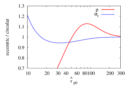
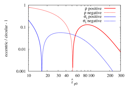
First, we demonstrate the dependence of and as full values, i.e. those obtained after all the radiation are detected, on the initial periapsis distance in Fig. 2. For comparison, all the values are normalized with respect to those of a circular binary, which take and ms for a binary at Mpc. Fig. 3 shows the relative difference in the logarithmic scale, and representative values for selected eccentric binaries as well as those for circular binaries are shown in Table 1.
The SNR, , takes the largest value at . This increase of the SNR at moderately large is primarily ascribed to the fact that the radiated energy tends to concentrate around sensitive frequency of a particular detector configuration. In contrast, the SNR decreases at smaller values of , because the initial orbit is too close to the last stable orbit and contribution from the inspiral phase at a large separation is lost. For a large value of , the SNR is essentially the same as that of a circular binary. This figure implies that the horizon distance is changed only up to a few tens per cent for eccentric binaries except for those born with very small . We do not pay particular attention to such a weak signal regime in this study.
The timing accuracy for an eccentric binary with is better than that for a circular binary, and it approaches the value for a circular binary at large . We stress that the values for eccentric and circular binaries agree when we focus only on the reference time, and the results deviate even in the limit of when we also consider the reference phase. The timing accuracy becomes worse than that of the circular binary at due to the lack of the SNR, and we do not pay attention to that regime. The best timing accuracy is achieved at , whereas the SNR is smaller by 30 per cent than the circular value.
| (s) | ||
|---|---|---|
| 40 | 12.4 | 67.7 |
| 100 | 16.0 | 70.7 |
| 300 | 14.3 | 71.7 |
| 14.2 | 71.8 |
 |
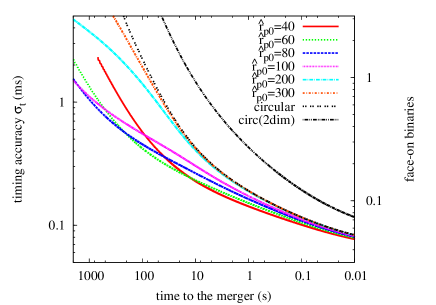 |
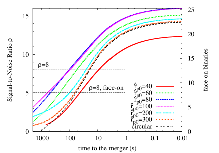
Next, we compare time evolution of and between eccentric and circular binaries. Fig. 4 shows the time evolution of and for various values of as well as those for a circular binary at Mpc. As an eyeguide, we include horizontal lines which denote both for the orientation-averaged and face-on binaries. Here, we also show the scale for face-on binaries, because the short-hard gamma-ray burst should be more relevant for such cases.
The comparison of the SNR evolution shows that eccentric binary coalescences accumulate SNRs from earlier stages of their lifetimes. A circular binary at Mpc achieves only at 20 s before the merger. By contrast, an eccentric binary with does at 100 s before the merger, partly due to the large full SNR but mainly due to strong emission at an early stage of its evolution. If we consider or of a face-on binary as a triggering criterion of the merger alert, it is achieved at 10 min before the merger for , whereas it is 1 min for a circular binary. The rapid SNR accumulation at a few minutes before the merger occurs approximately for . For a large value of , the accumulation behaviour of the SNR approach asymptotically to that of the circular case, because the dominant emission channel becomes the mode from a close orbit. For a small value of , the SNR is not substantial.
The time evolution of timing accuracy also depends on the value of . For a circular binary, ms is achieved at only 40 s before the merger with . By contrast, an eccentric binary with can achieve the same accuracy at 12 min before the merger. Roughly speaking, ms is achieved at a few minutes before the merger for . For virtually all the cases, the timing accuracy as a function of the time to the merger is always better for an eccentric binary than for a circular binary, while the SNR can be smaller for a small value of . This reflects the fact that the localization depends crucially on high-frequency gravitational waves, which a circular binary does not emit until right before the merger.
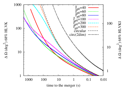
Finally, we compare time evolution of the localization accuracy between eccentric and circular binaries. Fig. 5 shows the evolution of localization accuracy for various values of as well as that for a circular binary. The localization area is shown as a sky position averaged value, and the best (worst) case values are obtained by multiplying 0.4 (3) and 0.5 (2.5) for four- and five-detector networks considered here, respectively (see Table 2). Although we specify a detector network, we do not take directional dependence of the antenna pattern function of each detector into account, and we take the same values of at all the detectors for simplicity. These values depend on the orientation and sky position of the binary and also orientation of the detector in reality. Especially, adopting the same values in all the detectors does not give realistic results for cases in which a binary is located on blind spots of detectors. Thus, this figure should not be taken too quantitatively, while we believe that this approximation is sufficient to demonstrate the localization efficiency.
This figure suggests that eccentric binaries could be localized with 68 per cent confidence up to 10 deg2, typical field of view of large-area optical telescopes (Nissanke et al., 2013), at half a minute before the merger by a four-detector network. On the other hand, a circular binary can be localized up to this accuracy only at a few seconds before the merger. If lower confidence and/or larger localization error are allowed for the purpose of sounding merger alerts, more rapid localization is possible.
Taking the expected latency for a gravitational-wave data analysis pipeline, one interesting value may be those at 10 min before the merger, at which , ms and 100 deg2 at 68 per cent confidence level are achieved. This should be contrasted with very large localization error for a circular binary, which will not enable us to declare that the source is localized in practice. The localization area is approximately halved if we restrict to 50 per cent confidence area, so that the five-detector network will be able to localize the source within 10 deg2 even at 10 min before the merger.
Overheads of electromagnetic instruments would determine the required time to the merger if the latency associated with gravitational-wave data analysis could be reduced (Cannon et al., 2012). They depend on particular instruments, and one possibility may be 1 min which can be achieved with robotic telescopes such as Robotic Transient Search Experiment (Rykoff et al., 2005). The SNR exceeds 8 for various values of , and the localization accuracy could be 10 deg2 by the four-detector network with slightly lower confidence level than 68 per cent. This level of accuracy is expected only a few seconds before the merger for a circular binary. Although this assumption is too optimistic to be realistic, this reminds us that reducing the latency could have a practical impact on pre-merger localization accuracy of eccentric binaries.
The localization accuracy is better for a face-on binary, which may be a progenitor of an observable short-hard gamma-ray burst. The localization area for an eccentric binary is sufficient for typical gamma-ray satellites, such as Fermi Large Area Telescope (LAT), when is achieved for a face-on one. This occurs earlier by an order of magnitude for an eccentric binary than for a circular binary (see Fig. 4). Still, taking not very rapid 0.2 deg s-1 slew speed of Fermi-LAT into account, a gamma-ray satellite capable of rapid timing-of-opportunity observation will be invaluable even if the sensitivity is inferior to current ones, because gamma-ray bursts at Mpc should be extremely bright. The Large Size Telescopes of the Cherenkov Telescope Array will be able to perform rapid follow-up to observe more energetic photons at the GeV–TeV range, which may be able to distinguish mechanisms of the extended emission (Veres & Mészáros, 2013).
| HLV | HLVK | HLVI | HLVKI | |
|---|---|---|---|---|
| 68 per cent best | 160 | 47 | 58 | 34 |
| 68 per cent average | — | 120 | 120 | 76 |
| 68 per cent worst | — | 330 | 360 | 190 |
| 90 per cent best | 310 | 96 | 120 | 69 |
| 90 per cent average | — | 250 | 240 | 150 |
| 90 per cent worst | — | 660 | 720 | 380 |
5 summary and discussion
We showed that gravitational waves from moderately eccentric compact binary coalescences will not only accumulate a substantial SNR at a few to 10 min before the merger, but also allow us to determine the sky position before the merger to the extent that we never expect for circular compact binary coalescences. This unique property owes to higher mode gravitational waves emitted during the eccentric inspiral phase. The pre-merger localization could give us a way to observe the whole merger process and associated electromagnetic counterparts provided that the sum of the latency of sounding merger alerts and overheads of follow-up observation required by telescopes and satellites can be sufficiently reduced.
The gravitational radiation model adopted in this study is derived by the quadrupole formula with Newtonian two-point orbital dynamics (Peters & Mathews, 1963; Peters, 1964). Post-Newtonian corrections such as the periastron precession and spin-orbit interaction have to be taken into account for more quantitative study and actual data analysis (Brown & Zimmerman, 2010; Huerta & Brown, 2013), although theoretical templates of gravitational waves from eccentric compact binary coalescences are not developed very much compared to those for circular ones (e.g. Gopakumar & Schäfer 2011; Tessmer & Schäfer 2011). Tidal effects due to the finite size of neutron stars, such as the excitation of f-mode oscillation, will also become important at some stage of the orbital evolution (Stephens et al., 2011; Gold et al., 2012; East & Pretorius, 2012). We expect that these issues modify our conclusion only quantitatively, because the repeated pulse-like waveform at the early stage of inspiral is conserved. Another assuring point is that the waveform near the merger is irrelevant to the purpose of the pre-merger localization and merger alert, and thus higher order post-Newtonian and tidal effects should be safely neglected.444But see, e.g. Loutrel et al. (2014) for possible “negative” post-Newtonian terms in modified gravity with dipolar radiation. As stated repeatedly, discontinuous orbital evolution in the high-eccentricity regime will require more careful consideration.
The timing triangulation approximation adopted in this study relies on the Fisher analysis, and it inevitably breaks down when we try to sound a merger alert using low SNR gravitational waves from a binary long before the merger. A detailed study such as Monte Carlo simulations is necessary to assess quantitatively the ability to localize the gravitational-wave source before the merger with low SNR signals. One important difference of the eccentric waveform from the circular one is the introduction of a new degree of freedom, which may be expressed as the angle of the periapsis direction (Barack & Cutler, 2004). The correlation between this angle and timing accuracy has to be investigated quantitatively, whereas we expect that the timing accuracy primarily depends on the pulse-like waveform structure. In addition, a common value of the timing accuracy (and SNR) is adopted for all the detectors to derive the localization accuracy, and this approximation requires improvement.
A challenging task will be the matched filtering analysis for long-term gravitational-wave pulse sequences (see also Antonini et al. (2014)).555See Tai et al. (2014) for an alternative approach to detect signals from eccentric compact binary coalescences. In a pipeline of initial LIGO-Virgo data analysis, detector output data are usually split into 256 s segments (Babak et al., 2013). This will be lengthened in a pipeline of second-generation detectors, which are sensitive at lower frequency. The required segment length will be, however, much longer for eccentric binaries than for circular binaries if we try to process all the available information, because eccentric binaries emit detectable gravitational waves during their early lives with very low orbital frequency (see the end of section 2). One way to overcome this is to develop a longer pipeline specialized to eccentric compact binary coalescences. The rotation of the earth will not be negligible with this strategy. Another way is to choose an appropriate time interval from the entire lifetime of an eccentric binary for a given length of the segment. The large number of harmonic modes can be a difficulty in practical construction of template banks without any dimensional reduction irrespective of the strategy.
The gravitational-wave pulse from an eccentric binary more resembles a detector glitch than the chirp signal from circular binaries does. Sequences of pulses may be naturally distinguished from noises by multidetector coincidences with information of timing consistency, and it might require human validation processes at least in the early epoch of second-generation gravitational-wave detectors. If high false alarm rates are allowed for the purpose of merger alerts to electromagnetic follow-up observations, omitting time consuming validation processes might be an option. Another, possibly ambitious, way to reduce effective latency might be to first carefully analyse gravitational-wave signals sufficiently before the merger aiming at rejecting false alarms, and next analyse signals as close to the merger as possible assuming that the signal is physical with available information from the first stage of analysis.
Acknowledgements
KK is deeply grateful to John L. Friedman for valuable discussions. KK is supported by JSPS Postdoctoral Fellowship for Research Abroad, and NS is supported by JSPS (24540269) and MEXT (24103006).
Appendix A Fisher analysis
We compute the Fisher information matrix with respect to and , where Greek indices take for or for . Using the fact that the nth harmonic mode is proportional to in the frequency domain, we can replace differentiation with respect to and by multiplication of and , respectively (Cutler & Flanagan, 1994). Components of the Fisher matrix are given by
| (30) | ||||
| (31) | ||||
| (32) |
Computing the inverse of this two-dimensional Fisher information matrix, we obtain the expression of the timing accuracy,
| (33) |
Note that for a circular binary emitting only via the mode, this expression gives
| (34) |
where is the effective bandwidth for single, mode gravitational waves. This result agrees with the one derived in Fairhurst (2009).
Now, let us confirm the divergence of phase-related components using a simplified detector model characterized by
| (35) |
where is a constant. The SNR is given by
| (36) |
and thus, we have
| (37) |
Hereafter, we replace by an integral and express the luminosity in a more convenient form as
| (38) |
In the limit of , we have
| (39) | ||||
| (40) | ||||
| (41) | ||||
| (42) | ||||
| (43) |
Therefore, the SNR is approximately written as
| (44) |
Now we can relate and by as
| (45) |
and we can derive (Olver, 1954)
| (46) |
at the limit of (). Finally, we have
| (47) |
Thus, the integral (or originally the summation) of is not divergent at , so is . The integral for diverges but as moderate as . The integral for is , and thus violent.
References
- Abadie et al. (2012) Abadie J. et al., 2012, A&A, 539, A124
- Accadia et al. (2011) Accadia T. et al., 2011, Class. Quantum Gravity, 28, 025005
- Antognini et al. (2014) Antognini J. M., Shappee B. J., Thompson T. A., Amaro-Seoane P., 2014, MNRAS, 439, 1079
- Antonini & Perets (2012) Antonini F., Perets H. B., 2012, ApJ, 757, 27
- Antonini et al. (2014) Antonini F., Murray N., Mikkola S., 2014, ApJ, 781, 45
- Babak et al. (2013) Babak S. et al., 2013, Phys. Rev. D, 87, 024033
- Barack & Cutler (2004) Barack L., Cutler C., 2004, Phys. Rev. D, 69, 082005
- Berger (2013) Berger E., 2013, preprint (arXiv:1311.2603)
- Berger et al. (2013) Berger E., Fong W., Chornock R., 2013, ApJ, 774, L23
- Bionta et al. (1987) Bionta R. M., Blewitt G., Bratton C. B., Casper D., Ciocio A., 1987, Phys. Rev. Lett., 58, 1494
- Brown & Zimmerman (2010) Brown D. A., Zimmerman P. J., 2010, Phys. Rev. D, 81, 024007
- Cannon et al. (2012) Cannon K. et al., 2012, ApJ, 748, 136
- Cutler & Flanagan (1994) Cutler C., Flanagan É. É., 1994, Phys. Rev. D, 49, 2658
- Cutler et al. (1994) Cutler C., Kennefick D., Poisson E., 1994, Phys. Rev. D, 50, 3816
- East & Pretorius (2012) East W. E., Pretorius F., 2012, ApJ, 760, L4
- East et al. (2013) East W. E., McWilliams S. T., Levin J., Pretorius F., 2013, Phys. Rev. D, 87, 043004
- Evans et al. (2012) Evans P. A. et al., 2012, ApJS, 203, 28
- Fairhurst (2009) Fairhurst S., 2009, New J. Phys., 11, 123006
- Fairhurst (2011) Fairhurst S., 2011, Class. Quantum Gravity, 28, 105021
- Flanagan & Hughes (1998) Flanagan É. É., Hughes S. A., 1998, Phys. Rev. D, 57, 4535
- Gold et al. (2012) Gold R., Bernuzzi S., Thierfelder M., Brügmann B., Pretorius F., 2012, Phys. Rev. D, 86, 121501
- Gopakumar & Schäfer (2011) Gopakumar A., Schäfer G., 2011, Phys. Rev. D, 84, 124007
- Grover et al. (2014) Grover K., Fairhurst S., Farr B. F., Mandel I., Rodriguez C., Sidery T., Vecchio A., 2014, Phys. Rev. D, 89, 042004
- Harry & LIGO Scientific Collaboration (2010) Harry G. M., LIGO Scientific Collaboration, 2010, Class. Quantum Gravity, 27, 084006
- Hirata et al. (1987) Hirata K., Kajita T., Koshiba M., Nakahata M., Oyama Y., 1987, Phys. Rev. Lett., 58, 1490
- Hotokezaka et al. (2013) Hotokezaka K., Kyutoku K., Tanaka M., Kiuchi K., Sekiguchi Y., Shiata M., Wanajo S., 2013, ApJ, 778, L16
- Huerta & Brown (2013) Huerta E. A., Brown D. A., 2013, Phys. Rev. D, 87, 127501
- Kasliwal & Nissanke (2013) Kasliwal M., Nissanke S., 2013, preprint (arXiv:1309.1554)
- Kocsis & Levin (2012) Kocsis B., Levin J., 2012, Phys. Rev. D, 85, 123005
- Kyutoku et al. (2014) Kyutoku K., Ioka K., Shibata M., 2014, MNRAS, 437, L6
- Lee et al. (2010) Lee W. E., Ramirez-Ruiz E., van de Ven G., 2010, ApJ, 720, 953
- LIGO Scientific Collaboration and Virgo Collaboration (2013) LIGO Scientific Collaboration and Virgo Collaboration, 2013, preprint (arXiv:1304.0670)
- Loutrel et al. (2014) Loutrel N., Yunes N., Pretorius F., 2014, preprint (arXiv:1404.0092)
- Metzger & Berger (2012) Metzger B. D., Berger E., 2012, ApJ, 746, 48
- Nakamura et al. (2013) Nakamura T., Kashiyama K., Nakauchi D., Suwa Y., Sakamoto T., Kawai N., 2013, preprint (arXiv:1312.0297)
- Nakar (2007) Nakar E., 2007, Phys. Rep., 442, 166
- Nissanke et al. (2013) Nissanke S., Kasliwal M., Georgieva A., 2013, ApJ, 767, 124
- Nuttall & Sutton (2010) Nuttall L. K., Sutton P. J., 2010, Phys. Rev. D, 82, 102002
- O’Leary et al. (2009) O’Leary R. M., Kocsis B., Loeb A., 2009, MNRAS, 395, 2127
- Olver (1954) Olver F. W. J., 1954, Phil. Trans. R. Soc. A, 247, 328
- Peters (1964) Peters P. C., 1964, Phys. Rev., 136, B1224
- Peters & Mathews (1963) Peters P. C., Mathews J., 1963, Phys. Rev., 131, 435
- Piran et al. (2013) Piran T., Nakar E., Rosswog S., 2013, MNRAS, 430, 2121
- Rykoff et al. (2005) Rykoff E. S. et al., 2005, ApJ, 631, L121
- Samsing et al. (2014) Samsing J., Macleod M., Ramirez-Ruiz E., 2014, ApJ., 784, 71
- Schutz (1986) Schutz B. F., 1986, Nature, 323, 310
- Schutz (2011) Schutz B. F., 2011, Class. Quantum Gravity, 28, 125023
- Seto (2013) Seto N., 2013, Phys. Rev. Lett., 111, 061106
- Somiya (2012) Somiya K., 2012, Class. Quantum Gravity, 29, 124007
- Stephens et al. (2011) Stephens B. C., East W. E., Pretorius F., 2011, ApJ, 737, L5
- Tai et al. (2014) Tai K. S., McWilliams S. T., Pretorius F., 2014, preprint (arXiv:1403.7754)
- Tanvir et al. (2013) Tanvir N. R., Levan A. J., Fruchter A. S., Hjorth J., Hounsell R., Wiersema K., Tunnicliffe R. L., 2013, Nature, 500, 547
- Tessmer & Schäfer (2011) Tessmer M., Schäfer G., 2011, Ann. Phys., 523, 813
- Tsang (2013) Tsang D., 2013, ApJ, 777, 103
- Veres & Mészáros (2013) Veres P., Mészáros P., 2013, preprint (arXiv:1312.0590)