Semileptonic B→D∗∗bold-â†’đ”superscriptđ·absent\boldsymbol{B\to D^{**}} decays in Lattice QCD : a feasability study and first results

M Atouib, B. Blossiera, V. Morénasb
O. PĂšnea, K. Petrovc
Abstract

We compute the decays B→D0âˆ—â†’đ”subscriptsuperscriptđ·âˆ—0{B\to D^{\ast}_{0}} and B→D2âˆ—â†’đ”subscriptsuperscriptđ·âˆ—2{B\to D^{\ast}_{2}} with finite masses for the b𝑏b and c𝑐c quarks. We first discuss the spectral properties of both the Bđ”B meson as a function of its momentum and of the D0∗subscriptsuperscriptđ·âˆ—0D^{\ast}_{0} and D2∗subscriptsuperscriptđ·âˆ—2D^{\ast}_{2} at rest. We compute the theoretical formulae leading to the decay amplitudes from the three-point and two-point correlators. We then compute the amplitudes at zero recoil of B→D0âˆ—â†’đ”subscriptsuperscriptđ·âˆ—0{B\to D^{\ast}_{0}} which turns out not to be vanishing contrary to what happens in the heavy quark limit. This opens a possibility to get a better agreement with experiment. To improve the continuum limit we have added a set of data with smaller lattice spacing. The B→D2âˆ—â†’đ”subscriptsuperscriptđ·âˆ—2{B\to D^{\ast}_{2}} vanishes at zero recoil and we show a convincing signal but only slightly more than 1 sigma from 0. In order to reach quantitatively significant results, we plan to fully exploit smaller lattice spacings as well as another lattice regularization.

[Uncaptioned image]

a Laboratoire de Physique Théorique111Unité Mixte de Recherche 8627 du Centre National de la Recherche Scientifique,

CNRS et Université Paris-Sud XI, Bùtiment 210, 91405 Orsay Cedex, France

b Laboratoire de Physique Corpusculaire de Clermont-Ferrand222Unité Mixte de Recherche 6533 CNRS/IN2P3 - Université Blaise Pascal, Campus Universitaire des Cézeaux,

4 avenue Blaise Pascal, TSA 60026, CS 60026, 63178 AubiĂšre Cedex, France

cInria Saclay, 1 rue HonorĂ© d’Estienne d’Orves, BĂątiment Alan Turing,

Campus de l’Ecole Polytechnique, 91120 Palaiseau, France

LPC-Clermont RI 13-07

LPT-Orsay-13-101

1 Introduction

Understanding the composition of the final state in Bđ”B meson semileptonic decay into charm meson is of key importance to control the theoretical error on the CKM matrix element Vc​bsubscript𝑉𝑐𝑏V_{cb}. The discrepancy between the inclusive determination and the exclusive one, based on B→D(∗)​lâ€‹Îœâ†’đ”superscriptđ·đ‘™đœˆB\to D^{(*)}l\nu, is still of the order of 3ÏƒđœŽ\sigma [1]. A significant part of the total width Γ​(B→Xc​l​Μ)Î“â†’đ”subscript𝑋𝑐𝑙𝜈\Gamma(B\to X_{c}l\nu) comes from excited states: it was recently argued that the radial excitation Dâ€Čsuperscriptđ·â€ČD^{\prime} might be particularly favoured, implying a suppression of the B→Dâˆ—â†’đ”superscriptđ·B\to D^{*} form factors as suggested by a study performed using the Operator Product Expansion formalism [2]. Another group of states that contribute to the width, about one quarter of it, is orbital excitations, in other words, positive parity charmed mesons, that we will note D∗∗superscriptđ·absentD^{**} hereafter. They are not well understood: indeed there seems to be a persistent discrepancy between claims from theory and from experiment [3], while a comparison between semileptonic decay and non leptonic decay B→Dâˆ—âˆ—â€‹Ï€â†’đ”superscriptđ·absent𝜋B\to D^{**}\pi, involving the same form factors (at least in the case of the so-called Class I process), is quite confusing on the experimental side [4]. Two types of D∗∗superscriptđ·absentD^{**} are observed: two “narrow resonances” D3/2subscriptđ·32D_{3/2} and a couple of “broad resonances” D1/2subscriptđ·12D_{1/2}, in the same mass region [5]. While experiments point towards a dominance of the broad resonances in semileptonic decays, theory points rather towards a dominance of the narrow resonances : not only a series of sum rules [6, 7] derived from QCD obtains that hierarchy, but also calculations with quark models [8] - [10] and lattice computations performed in the quenched approximation [11] and with Nf=2subscriptNf2{\rm N_{f}}=2 dynamical quarks [12]. However, the main limitation of these results is that they are derived in the heavy quark limit. 1/mc1subscript𝑚𝑐1/m_{c} corrections might be pretty large and, before getting any definitive conclusion on the disagreement between theory and experiment in that sector of flavour physics, it is mandatory to reduce the sources of systematic errors on the theory side.

2 Theoretical framework

In this paragraph, all the main formulae up to the differential decay rates will be given for the semileptonic decays of a Bđ”B heavy meson into the first orbitally excited D∗∗superscriptđ·absentD^{**} mesons.

We will focus our study on the production of the |P03⟩delimited-|⟩superscriptsubscript𝑃03\big{\lvert}\prescript{3}{}{P}_{0}\big{\rangle} (scalar D0∗subscriptsuperscriptđ·0D^{*}_{0}) and the |P23⟩delimited-|⟩superscriptsubscript𝑃23\big{\lvert}\prescript{3}{}{P}_{2}\big{\rangle} (tensor D2∗subscriptsuperscriptđ·2D^{*}_{2}) states333We use the |LJ2​S+1⟩delimited-|⟩superscriptsubscriptđżđœ2𝑆1\big{\lvert}\prescript{2S+1}{}{L}_{J}\big{\rangle} notation of the states, where S𝑆S is the spin angular momentum, L=1𝐿1L=1 the orbital angular momentum and J=L+Sđœđżđ‘†J=L+S the total angular momentum of the D∗∗superscriptđ·absentD^{**} state..

Finally, we will also give relations in the case where the mass of the lepton cannot be neglected.

2.1 Form factors

In order to derive the decay rates, we need the transition amplitudes. They can be described using 6 form factors [15].

P23superscriptsubscript𝑃23\prescript{3}{}{P}_{2} state :

⟹P23​(pD2∗,Δ​(pD2∗,λ))|VÎŒ|B​(pB)⟩quantum-operator-productsuperscriptsubscript𝑃23subscript𝑝subscriptsuperscriptđ·2𝜀subscript𝑝subscriptsuperscriptđ·2𝜆subscriptđ‘‰đœ‡đ”subscriptđ‘đ”\displaystyle\big{\langle}\prescript{3}{}{P}_{2}\bigl{(}p_{{}_{\!D^{*}_{2}}},\,\varepsilon(p_{{}_{\!D^{*}_{2}}},\,\lambda)\bigr{)}\,\big{|}\,V_{\mu}\,\big{|}\,B(p_{{}_{\!B}})\big{\rangle} =i​h~​ϔΌ​Μ​λ​ρ​Δ(pD2∗,λ)∗Μ​α​pBα​(pB+pD2∗)λ​(pB−pD2∗)ρabsent𝑖~ℎsubscriptitalic-Ï”đœ‡đœˆđœ†đœŒsubscriptsuperscript𝜀∗absentđœˆđ›Œsubscript𝑝subscriptsuperscriptđ·2𝜆subscriptsubscriptđ‘đ”đ›Œsuperscriptsubscriptđ‘đ”subscript𝑝subscriptsuperscriptđ·2𝜆superscriptsubscriptđ‘đ”subscript𝑝subscriptsuperscriptđ·2𝜌\displaystyle=\ i\,\boxed{\tilde{h}}\,\epsilon_{\mu\nu\lambda\rho}\,\varepsilon^{\ast\nu\alpha}_{(p_{{}_{\!D^{*}_{2}}},\,\lambda)}\,{p_{{}_{\!B}}}_{\alpha}\,(p_{{}_{\!B}}+{p_{{}_{\!D^{*}_{2}}}})^{\lambda}\,(p_{{}_{\!B}}-{p_{{}_{\!D^{*}_{2}}}})^{\rho} (2.1)
⟹P23​(pD2∗,Δ​(pD2∗,λ))|AÎŒ|B​(pB)⟩quantum-operator-productsuperscriptsubscript𝑃23subscript𝑝subscriptsuperscriptđ·2𝜀subscript𝑝subscriptsuperscriptđ·2𝜆subscriptđŽđœ‡đ”subscriptđ‘đ”\displaystyle\big{\langle}\prescript{3}{}{P}_{2}\bigl{(}p_{{}_{\!D^{*}_{2}}},\,\varepsilon(p_{{}_{\!D^{*}_{2}}},\,\lambda)\bigr{)}\,\big{|}\,A_{\mu}\,\big{|}\,B(p_{{}_{\!B}})\big{\rangle} =k~​ΔΌ​Μ∗(pD2∗,λ)​pBÎœ+(Δα​ÎČ∗(pD2∗,λ)​pBα​pBÎČ)​[b~+​(pB+pD2∗)ÎŒ+b~−​(pB−pD2∗)ÎŒ]absent~𝑘superscriptsuperscriptsubscript𝜀𝜇𝜈∗subscript𝑝subscriptsuperscriptđ·2𝜆superscriptsubscriptđ‘đ”đœˆsuperscriptsuperscriptsubscriptđœ€đ›Œđ›œâˆ—subscript𝑝subscriptsuperscriptđ·2𝜆superscriptsubscriptđ‘đ”đ›Œsuperscriptsubscriptđ‘đ”đ›œdelimited-[]subscript~𝑏subscriptsubscriptđ‘đ”subscript𝑝subscriptsuperscriptđ·2𝜇subscript~𝑏subscriptsubscriptđ‘đ”subscript𝑝subscriptsuperscriptđ·2𝜇\displaystyle=\boxed{\tilde{k}}\,{\varepsilon_{\mu\nu}^{\ast}}^{\!\!\!\!(p_{{}_{\!D^{*}_{2}}},\,\lambda)}{p_{{}_{\!B}}}^{\nu}+\left({{\varepsilon_{\alpha\beta}^{\ast}}^{\!\!\!\!(p_{{}_{\!D^{*}_{2}}},\,\lambda)}{p_{{}_{\!B}}}^{\alpha}{p_{{}_{\!B}}}^{\beta}}\right)\left[{\boxed{\tilde{b}_{+}}\,(p_{{}_{\!B}}+p_{{}_{\!D^{*}_{2}}})_{\mu}+\boxed{\tilde{b}_{-}}\,(p_{{}_{\!B}}-p_{{}_{\!D^{*}_{2}}})_{\mu}}\right]

P03superscriptsubscript𝑃03\prescript{3}{}{P}_{0} state :

⟹P03​(pD0∗)|VÎŒ|B​(pB)⟩quantum-operator-productsuperscriptsubscript𝑃03subscript𝑝subscriptsuperscriptđ·0subscriptđ‘‰đœ‡đ”subscriptđ‘đ”\displaystyle\big{\langle}\prescript{3}{}{P}_{0}(p_{{}_{\!D^{*}_{0}}})\,\big{|}\,V_{\mu}\,\big{|}\,B(p_{{}_{\!B}})\big{\rangle} =0(parity invariance)absent0(parity invariance)\displaystyle=0\qquad\quad\text{(parity invariance)} (2.2)
⟹P03​(pD0∗)|AÎŒ|B​(pB)⟩quantum-operator-productsuperscriptsubscript𝑃03subscript𝑝subscriptsuperscriptđ·0subscriptđŽđœ‡đ”subscriptđ‘đ”\displaystyle\big{\langle}\prescript{3}{}{P}_{0}(p_{{}_{\!D^{*}_{0}}})\,\big{|}\,A_{\mu}\,\big{|}\,B(p_{{}_{\!B}})\big{\rangle} =u~+​(pB+pD0∗)ÎŒ+u~−​(pB−pD0∗)ÎŒabsentsubscript~𝑱subscriptsubscriptđ‘đ”subscript𝑝subscriptsuperscriptđ·0𝜇subscript~𝑱subscriptsubscriptđ‘đ”subscript𝑝subscriptsuperscriptđ·0𝜇\displaystyle=\boxed{\tilde{u}_{+}}\,(p_{{}_{\!B}}+p_{{}_{\!D^{*}_{0}}})_{\mu}+\boxed{\tilde{u}_{-}}\,(p_{{}_{\!B}}-p_{{}_{\!D^{*}_{0}}})_{\mu}

where VÎŒsubscript𝑉𝜇V_{\mu} denotes the vector current cÂŻâ€‹ÎłÎŒâ€‹b¯𝑐subscriptđ›Ÿđœ‡đ‘\bar{c}\gamma_{\mu}b and AÎŒsubscript𝐮𝜇A_{\mu} the axial current cÂŻâ€‹ÎłÎŒâ€‹Îł5​b¯𝑐subscriptđ›Ÿđœ‡subscriptđ›Ÿ5𝑏\bar{c}\gamma_{\mu}\gamma_{5}b.

Δ​(pD2∗,λ)𝜀subscript𝑝subscriptsuperscriptđ·2𝜆\varepsilon(p_{{}_{\!D^{*}_{2}}},\,\lambda) is the polarisation tensor of the P23superscriptsubscript𝑃23\prescript{3}{}{P}_{2} state (Î»đœ†\lambda being the projection of the J=2đœ2J=2 total angular momentum along some quantification axis).

Moreover, the chosen normalisation of the mesonic states is

⟹M​(pâ€Č)|M​(p)⟩=(2​π)3​ 2​E​ή3​(p→â€Č−p→).inner-product𝑀superscript𝑝â€Č𝑀𝑝superscript2𝜋32𝐾superscript𝛿3superscript→𝑝â€Č→𝑝\big{\langle}M\bigl{(}p^{\,\prime}\bigr{)}\,\big{|}\,M\bigl{(}p\bigr{)}\big{\rangle}\ =\ (2\pi)^{3}\,2E\,\delta^{3}(\vec{p}^{\,\prime}-\vec{p})\,.

Finally, because of parity and time-reversal invariance of the strong interactions, those form factors are real numbers.

2.2 Differential decay rates

The goal is to compute the differential decay width d​Γ​(B¯→Dâˆ—âˆ—â€‹â„“â€‹ÎœÂŻ)dÎ“â†’ÂŻđ”superscriptđ·absentℓ¯𝜈\text{d}\Gamma(\bar{B}\to D^{**}\,\ell\,\bar{\nu}) whose general expression is

d​Γ​(B¯→Dâˆ—âˆ—â€‹â„“â€‹ÎœÂŻ)=12​EB​|ℳ¯|2​d​Ω,dÎ“â†’ÂŻđ”superscriptđ·absentℓ¯𝜈12subscriptđžđ”superscript¯ℳ2dΊ\displaystyle\text{d}\Gamma(\bar{B}\to D^{**}\,\ell\,\bar{\nu})=\dfrac{1}{2\,E_{{}_{\!B}}}\,\lvert\bar{\mathscr{M}}\rvert^{2}\,\text{d}\Phi\,,
with{d​Ω=d3​p→D∗∗(2​π)3​ 2​ED∗∗​d3​p→ℓ(2​π)3​ 2​Eℓ​d3​p→Μ(2​π)3​ 2​EΜ​(2​π)4​ή(4)​(pB−pD∗∗−pℓ−pÎœ),|ℳ¯|2=∑Ό,ÎœWΌ​Μ​ℓΌ​Μ.\displaystyle\text{with}\qquad\qquad\left\{\begin{aligned} &\text{d}\Phi=\dfrac{d^{3}\vec{p}_{{}_{\!D^{**}}}}{(2\pi)^{3}\,2E_{{}_{\!D^{**}}}}\,\dfrac{d^{3}\vec{p}_{{}_{\!\ell}}}{(2\pi)^{3}\,2E_{{}_{\!\ell}}}\,\dfrac{d^{3}\vec{p}_{{}_{\!\nu}}}{(2\pi)^{3}\,2E_{{}_{\!\nu}}}\,(2\pi)^{4}\,\delta^{(4)}(p_{{}_{\!B}}-p_{{}_{\!D^{**}}}-p_{{}_{\!\ell}}-{p}_{{}_{\!\nu}})\,,\\[5.69054pt] &\lvert\bar{\mathscr{M}}\rvert^{2}=\sum\limits_{\mu,\,\nu}\,W_{\mu\nu}\ell^{\mu\nu}\,.\end{aligned}\right.

In the last equality, WΌ​Μsubscript𝑊𝜇𝜈W_{\mu\nu} denotes the hadronic tensor

WΌ​Μ​(pB,pD∗∗)=GF2​|Vc​b|22​∑final spins⟹D∗∗​(pD∗∗)|VΌ−AÎŒ|B¯​(pB)⟩​⟚B¯​(pB)|VΜ−AÎœ|D∗∗​(pD∗∗)⟩,subscript𝑊𝜇𝜈subscriptđ‘đ”subscript𝑝superscriptđ·absentsuperscriptsubscriptđșđč2superscriptsubscript𝑉𝑐𝑏22subscriptfinal spinsquantum-operator-productsuperscriptđ·âˆ—absent∗subscript𝑝superscriptđ·absentsubscript𝑉𝜇subscriptđŽđœ‡ÂŻđ”subscriptđ‘đ”quantum-operator-productÂŻđ”subscriptđ‘đ”subscript𝑉𝜈subscript𝐮𝜈superscriptđ·âˆ—absent∗subscript𝑝superscriptđ·absentW_{\mu\nu}(p_{{}_{\!B}},\,p_{{}_{\!D^{**}}})=\dfrac{G_{F}^{2}\,\lvert V_{cb}\rvert^{2}}{2}\,\sum_{\mathclap{{\text{\tiny final spins}}}}\ \big{\langle}D^{\ast\ast}(p_{{}_{\!D^{**}}})\,\big{|}\,V_{\mu}-A_{\mu}\,\big{|}\,\bar{B}(p_{{}_{\!B}})\big{\rangle}\ \big{\langle}\bar{B}(p_{{}_{\!B}})\,\big{|}\,V_{\nu}-A_{\nu}\,\big{|}\,D^{\ast\ast}(p_{{}_{\!D^{**}}})\big{\rangle}\,,

where the transition amplitudes have been given in the preceding paragraph (let us note that there are no summation nor average over the initial spins since the BÂŻÂŻđ”\bar{B} meson has a spin equal to zero) and ℓΌ​Μsuperscriptℓ𝜇𝜈\ell^{\mu\nu} represents the leptonic tensor

ℓΌ​Μ​(pℓ,pÎœ)=∑s[u¯ℓ​(pℓ,s)â€‹ÎłÎŒâ€‹(1−γ5)​vΜ​(pÎœ)]⋅[u¯ℓ​(pℓ,s)â€‹ÎłÎœâ€‹(1−γ5)​vΜ​(pÎœ)]∗superscriptℓ𝜇𝜈subscript𝑝ℓsubscript𝑝𝜈subscript𝑠⋅delimited-[]subscript¯𝑱ℓsubscript𝑝ℓ𝑠superscriptđ›Ÿđœ‡1superscriptđ›Ÿ5subscript𝑣𝜈subscript𝑝𝜈superscriptdelimited-[]subscript¯𝑱ℓsubscript𝑝ℓ𝑠superscriptđ›Ÿđœˆ1superscriptđ›Ÿ5subscript𝑣𝜈subscript𝑝𝜈∗\ell^{\mu\nu}(p_{{}_{\!\ell}},\,{p}_{{}_{\!\nu}})=\sum_{s}\left[{\bar{u}_{\ell}(p_{{}_{\!\ell}},s)\,\gamma^{\mu}\!\left({1-\gamma^{5}}\right)\!v_{\nu}({p}_{{}_{\!\nu}})}\right]\!\!\cdot\!\!\left[{\bar{u}_{\ell}(p_{{}_{\!\ell}},s)\,\gamma^{\nu}\!\left({1-\gamma^{5}}\right)\!v_{\nu}({p}_{{}_{\!\nu}})}\right]^{\ast}

In that last formula, uℓ​(pℓ,s)subscript𝑱ℓsubscript𝑝ℓ𝑠u_{\ell}(p_{{}_{\!\ell}},s) is the lepton ℓℓ\ell spinor (s𝑠s denotes the usual projection of its spin), while vΜ​(pÎœ)subscript𝑣𝜈subscript𝑝𝜈v_{\nu}({p}_{{}_{\!\nu}}) represents the antineutrino ÎœÂŻÂŻđœˆ\bar{\nu} spinor.

All that remains is to compute the leptonic tensor, then the hadronic tensor and the measure d​ΩdΩ\text{d}\Phi of the phase space in order to obtain the expressions of the differential decay widths.

2.2.1 Leptonic tensor ℓ𝝁​𝝂superscriptbold-ℓ𝝁𝝂\boldsymbol{\ell^{\mu\nu}}

The calculation is classical and straightforward, leading to

ℓΌ​Μ=8​[pℓΌ​pΜΜ+pℓΜ​pΜΌ−(pℓ⋅pÎœ)​gΌ​Μ−i​ϔΌ​Μ​ρ​σ​(pℓ)ρ​(pÎœ)σ].superscriptℓ𝜇𝜈8delimited-[]superscriptsubscript𝑝ℓ𝜇superscriptsubscript𝑝𝜈𝜈superscriptsubscript𝑝ℓ𝜈superscriptsubscript𝑝𝜈𝜇⋅subscript𝑝ℓsubscript𝑝𝜈superscript𝑔𝜇𝜈𝑖superscriptitalic-Ï”đœ‡đœˆđœŒđœŽsubscriptsubscript𝑝ℓ𝜌subscriptsubscript𝑝𝜈𝜎\ell^{\mu\nu}=8\left[{p_{{}_{\!\ell}}^{\mu}\,{p}_{{}_{\!\nu}}^{\nu}\ +\ p_{{}_{\!\ell}}^{\nu}\,{p}_{{}_{\!\nu}}^{\mu}\ -(p_{{}_{\!\ell}}\cdot{p}_{{}_{\!\nu}})\,g^{\mu\nu}\ -\ i\,\epsilon^{\mu\nu\rho\sigma}(p_{{}_{\!\ell}})_{\rho}({p}_{{}_{\!\nu}})_{\sigma}}\right]\,.

We can notice that the mass of the lepton has vanished, which renders the expression valid in the situations where mℓ=0subscript𝑚ℓ0m_{{}_{\!\ell}}=0 as well as mℓ≠0subscript𝑚ℓ0m_{{}_{\!\ell}}\neq 0.

2.2.2 Hadronic tensor đ‘Ÿđâ€‹đ‚subscriptđ‘Ÿđđ‚\boldsymbol{W_{\mu\nu}}

By looking at the expressions of the transition amplitudes given above, the general structure of the hadronic tensor can be inferred and put into the form [15]:

WΌ​Μ=GF2​|Vc​b|22[αgΌ​Μ+ÎČ++(pB+pD∗∗)ÎŒ(pB+pD∗∗)Îœ+ÎČ+−(pB+pD∗∗)ÎŒ(pB−pD∗∗)Îœ..+ÎČ−+(pB−pD∗∗)ÎŒ(pB+pD∗∗)Îœ+ÎČ−−(pB−pD∗∗)ÎŒ(pB−pD∗∗)Îœ+iÎłÏ”ÎŒâ€‹Îœâ€‹Ïâ€‹Ïƒ(pB+pD∗∗)ρ(pB−pD∗∗)σ].\begin{split}W_{\mu\nu}&=\dfrac{G_{F}^{2}\,\lvert V_{cb}\rvert^{2}}{2}\,\biggl{[}{\boxed{\alpha}\,g_{\mu\nu}\ +\ \boxed{\beta_{{}_{++}}}(p_{{}_{\!B}}+p_{{}_{\!D^{**}}})_{\mu}(p_{{}_{\!B}}+p_{{}_{\!D^{**}}})_{\nu}\ +\ \boxed{\beta_{{}_{+-}}}(p_{{}_{\!B}}+p_{{}_{\!D^{**}}})_{\mu}(p_{{}_{\!B}}-p_{{}_{\!D^{**}}})_{\nu}}\biggr{.}\\ &\biggl{.}{\ +\ \boxed{\beta_{{}_{-+}}}(p_{{}_{\!B}}-p_{{}_{\!D^{**}}})_{\mu}(p_{{}_{\!B}}+p_{{}_{\!D^{**}}})_{\nu}\ +\ \beta_{{}_{--}}(p_{{}_{\!B}}-p_{{}_{\!D^{**}}})_{\mu}(p_{{}_{\!B}}-p_{{}_{\!D^{**}}})_{\nu}\ +\ i\,\boxed{\gamma}\,\epsilon_{\mu\nu\rho\sigma}(p_{{}_{\!B}}+p_{{}_{\!D^{**}}})^{\rho}(p_{{}_{\!B}}-p_{{}_{\!D^{**}}})^{\sigma}}\biggr{]}\,.\end{split} (2.3)

The coefficients Î±đ›Œ{\alpha}, ÎČ++subscriptđ›œabsent{\beta_{{}_{++}}}, ÎČ+−subscriptđ›œabsent{\beta_{{}_{+-}}}, ÎČ−+subscriptđ›œabsent{\beta_{{}_{-+}}}, ÎČ−−subscriptđ›œabsent{\beta_{{}_{--}}} and Îłđ›Ÿ{\gamma} are given in the Appendix for the P03superscriptsubscript𝑃03\prescript{3}{}{P}_{0} and the P23superscriptsubscript𝑃23\prescript{3}{}{P}_{2} states.

2.2.3 Kinematics and notations

For reasons of simplification, we now choose to compute the decay rates in the rest frame of the BÂŻÂŻđ”\bar{B} meson.

We then define two dimensionless parameters xđ‘„x and y𝑩y according to

x​mB=2​Eâ„“đ‘„subscriptđ‘šđ”2subscript𝐾ℓ\boxed{x\,m_{{}_{\!B}}=2\,E_{{}_{\!\ell}}}
as well asy​mB2=(pB−pD∗∗)2=(pℓ+pÎœ)2as well as𝑩superscriptsubscriptđ‘šđ”2superscriptsubscriptđ‘đ”subscript𝑝superscriptđ·absent2superscriptsubscript𝑝ℓsubscript𝑝𝜈2\text{as well as}\qquad\qquad\qquad\boxed{y\,m_{{}_{\!B}}^{2}=(p_{{}_{\!B}}-p_{{}_{\!D^{**}}})^{2}=(p_{{}_{\!\ell}}+{p}_{{}_{\!\nu}})^{2}}

where Eℓsubscript𝐾ℓE_{{}_{\!\ell}} is the energy of the lepton in the BÂŻÂŻđ”\bar{B} rest frame.

We introduce also the mass ratio rXsubscript𝑟𝑋r_{{}_{\!X}}

mX=rX​mBwhere X is either a D∗∗ meson or the lepton ℓsubscript𝑚𝑋subscript𝑟𝑋subscriptđ‘šđ”where X is either a D∗∗ meson or the lepton ℓ\boxed{m_{{}_{\!X}}\ =\ r_{{}_{\!X}}\,{m_{{}_{\!B}}}}\qquad\text{where $X$ is either a $D^{**}$ meson or the lepton $\ell$}

Many kinematical terms can be expressed with these three parameters, such as

ED∗∗=mB2(1−y+rD∗∗2);pℓ⋅pÎœ=12mB2(y−rℓ2);pℓ⋅pD∗∗=12mB2(x−y−rℓ2);pB⋅pℓ=12mB2x.E_{{}_{\!D^{**}}}=\dfrac{m_{{}_{\!B}}}{2}\,(1-y+r_{{}_{\!D^{**}}}^{2})\quad;\quad p_{{}_{\!\ell}}\cdot{p}_{{}_{\!\nu}}=\dfrac{1}{2}\,m_{{}_{\!B}}^{2}\,(y-r_{{}_{\!\ell}}^{2})\quad;\quad p_{{}_{\!\ell}}\cdot p_{{}_{\!D^{**}}}=\dfrac{1}{2}\,m_{{}_{\!B}}^{2}\,(x-y-r_{{}_{\!\ell}}^{2})\quad;\quad p_{{}_{\!B}}\cdot p_{{}_{\!\ell}}=\dfrac{1}{2}\,m_{{}_{\!B}}^{2}\,x\quad.

2.2.4 Measure dâ€‹đšœdđšœ\boldsymbol{\text{d}\Phi} of the phase space

The goal is to get the differential widths d​ΓdΓ\text{d}\Gamma with respect to the lepton energy Eℓsubscript𝐾ℓE_{{}_{\!\ell}} and the momentum transfer (pB−pD∗∗)2superscriptsubscriptđ‘đ”subscript𝑝superscriptđ·absent2(p_{{}_{\!B}}-p_{{}_{\!D^{**}}})^{2}, in other words with respect to the variables xđ‘„x and y𝑩y : d2​Γ/d​x​d​ysuperscriptd2Γdđ‘„d𝑩\ {\text{d}^{2}\Gamma}/{\text{d}x\,\text{d}y}

So we must integrate over the antineutrino momentum p→Μsubscript→𝑝𝜈\vec{p}_{{}_{\!\nu}}, then over all possible orientations of p→ℓsubscript→𝑝ℓ\vec{p}_{{}_{\!\ell}} so that only the dependance on Eℓsubscript𝐾ℓE_{{}_{\!\ell}} (i.e. on xđ‘„x) remains, and finally over all possible directions of the 3-vector p→D∗∗subscript→𝑝superscriptđ·absent\vec{p}_{{}_{\!D^{**}}} since we want to keep the dependance on ED∗∗subscript𝐾superscriptđ·absentE_{{}_{\!D^{**}}} (i.e. on y𝑩y). We finally get :

d​Ω=−mB2128​π3​d​x​d​y​ξ​(1−x+y−rD∗∗2)dΊsuperscriptsubscriptđ‘šđ”2128superscript𝜋3dđ‘„d𝑩𝜃1đ‘„đ‘Šsuperscriptsubscript𝑟superscriptđ·absent2\text{d}\Phi=-\,\dfrac{m_{{}_{\!B}}^{2}}{128\pi^{3}}\,\text{d}x\,\text{d}y\,\theta(1-x+y-r_{{}_{\!D^{**}}}^{2})

where ξ​(z)𝜃𝑧\theta(z) is the usual Heaviside function.

2.2.5 Constraints on 𝒙𝒙\boldsymbol{x} and 𝒚𝒚\boldsymbol{y}

The parameters xđ‘„x and y𝑩y, that is the lepton energy (Eℓsubscript𝐾ℓE_{{}_{\!\ell}}) and the D∗∗superscriptđ·âˆ—absent∗D^{\ast\ast} meson energy (ED∗∗subscript𝐾superscriptđ·absentE_{{}_{\!D^{**}}}), cannot be arbitrary. They are constrained by two conditions : one which is obvious in the expression of d​ΩdΊ\text{d}\Phi above (the Heaviside function) and another one which appeared during the integration over the direction of p→ℓsubscript→𝑝ℓ\vec{p}_{{}_{\!\ell}}. In other terms, we have access to the variation domains of both parameters xđ‘„x and y𝑩y whether we consider x=x​(y)đ‘„đ‘„đ‘Šx=x(y) or y=y​(x)đ‘Šđ‘Šđ‘„y=y(x): they are given in the Appendix.

2.2.6 Differential decay widths in the đ‘©ÂŻbold-ÂŻđ‘©\boldsymbol{\bar{B}} rest frame

Using the definition of d​ΓdΓ\text{d}\Gamma as well as all the preceding results, the construction of the differential decay widths proceeds in the following way :

d​Γd​x​d​y​(B¯→Dâˆ—âˆ—â€‹â„“â€‹ÎœÂŻ)=−mB256​π3​|ℳ¯|2dΓdđ‘„dđ‘Šâ†’ÂŻđ”superscriptđ·absentℓ¯𝜈subscriptđ‘šđ”256superscript𝜋3superscript¯ℳ2\boxed{\dfrac{\text{d}\Gamma}{\text{d}x\,\text{d}y}(\bar{B}\to D^{**}\,\ell\,\bar{\nu})=-\,\dfrac{m_{{}_{\!B}}}{256\pi^{3}}\,\lvert\bar{\mathscr{M}}\rvert^{2}}

where |ℳ¯|2=WΌ​Μ​ℓΌ​Μsuperscript¯ℳ2subscript𝑊𝜇𝜈superscriptℓ𝜇𝜈\lvert\bar{\mathscr{M}}\rvert^{2}=W_{\mu\nu}\ell^{\mu\nu} becomes in this particular frame

|ℳ¯|2=2GF2|Vc​b|2mB2{.\displaystyle\lvert\bar{\mathscr{M}}\rvert^{2}=2\,{G_{F}^{2}\,\lvert V_{cb}\rvert^{2}}\,m_{{}_{\!B}}^{2}\,\Biggl{\{}{}\Biggr{.} −2​α​(y−rℓ2)2đ›Œđ‘Šsuperscriptsubscript𝑟ℓ2\displaystyle-2\,\boxed{\alpha}\,(y-r_{{}_{\!\ell}}^{2})
−ÎČ++​mB2​[4​[x​rD∗∗2+(1−x)​(y−x)]+rℓ2​[3​y−4​(x+rD∗∗2)+rℓ2]]subscriptđ›œabsentsuperscriptsubscriptđ‘šđ”2delimited-[]4delimited-[]đ‘„superscriptsubscript𝑟superscriptđ·absent21đ‘„đ‘Šđ‘„superscriptsubscript𝑟ℓ2delimited-[]3𝑩4đ‘„superscriptsubscript𝑟superscriptđ·absent2superscriptsubscript𝑟ℓ2\displaystyle-\boxed{\beta_{{}_{++}}}\,m_{{}_{\!B}}^{2}\,\Bigl{[}{4\,\bigl{[}{x\,r_{{}_{\!D^{**}}}^{2}+(1-x)(y-x)}\bigr{]}+r_{{}_{\!\ell}}^{2}\bigl{[}{3\,y-4(x+r_{{}_{\!D^{**}}}^{2})+r_{{}_{\!\ell}}^{2}}\bigr{]}}\Bigr{]}
+(ÎČ+−+ÎČ−+)​mB2​rℓ2​[2​(1−x−rD∗∗2)+y+rℓ2]subscriptđ›œabsentsubscriptđ›œabsentsuperscriptsubscriptđ‘šđ”2superscriptsubscript𝑟ℓ2delimited-[]21đ‘„superscriptsubscript𝑟superscriptđ·absent2𝑩superscriptsubscript𝑟ℓ2\displaystyle+\left({\,\boxed{\beta_{{}_{+-}}}+\boxed{\beta_{{}_{-+}}}\,}\right)\,m_{{}_{\!B}}^{2}\,r_{{}_{\!\ell}}^{2}\Bigl{[}{2(1-x-r_{{}_{\!D^{**}}}^{2})+y+r_{{}_{\!\ell}}^{2}}\Bigr{]}
+ÎČ−−​mB2​rℓ2​(y−rℓ2)subscriptđ›œabsentsuperscriptsubscriptđ‘šđ”2superscriptsubscript𝑟ℓ2𝑩superscriptsubscript𝑟ℓ2\displaystyle+\boxed{\beta_{{}_{--}}}\,m_{{}_{\!B}}^{2}\,r_{{}_{\!\ell}}^{2}\,(y-r_{{}_{\!\ell}}^{2})
−2γmB2[y(1+y−2x−rD∗∗2)+rℓ2(1+y−rD∗∗2)].}\displaystyle-2\,\boxed{\gamma}\,m_{{}_{\!B}}^{2}\Bigl{[}{y\,(1+y-2\,x-r_{{}_{\!D^{**}}}^{2})+r_{{}_{\!\ell}}^{2}(1+y-r_{{}_{\!D^{**}}}^{2})}\Bigr{]}\Biggl{.}{}\Biggr{\}}

We can notice that, for a zero mass lepton, only the coefficients Î±đ›Œ{\alpha}, ÎČ++subscriptđ›œabsent{\beta_{{}_{++}}} and Îłđ›Ÿ{\gamma} survive.

The expressions for each D∗∗superscriptđ·absentD^{**} are also written in the Appendix. However, their use requires the knowledge of the momentum dependance of the form factors. In the following, we will focus on a method to obtain such a dependance.

2.3 Extracting the form factors from the transition amplitudes

On the lattice, we compute the transition amplitudes for different momenta of the mesons. But we need the momentum dependance of the form factors in order to calculate the decay rates of the semileptonic decays of the Bđ”B to a D∗∗superscriptđ·absentD^{**}. So we must devise a way to extract the form factors from the lattice transition amplitudes.

2.3.1 Kinematics

We will work in the rest frame of the D∗∗superscriptđ·absentD^{**} meson444This will greatly simplify the calculations on the lattice. so the Bđ”B meson will carry the momentum. Moreover, we will consider the Bđ”B’s whose spatial momentum is symmetrical.

pD∗∗=(mD∗∗,0→)andpBÎŒ=(EB,p,p,p).formulae-sequencesubscript𝑝superscriptđ·absentsubscript𝑚superscriptđ·absent→0andsuperscriptsubscriptđ‘đ”đœ‡subscriptđžđ”đ‘đ‘đ‘p_{{}_{\!D^{**}}}=(m_{{}_{\!D^{**}}},\,\vec{0})\quad\quad\text{and}\quad\quad p_{{}_{\!B}}^{\mu}=(E_{{}_{\!B}},\,p,\,p,\,p)\quad.

We will also choose the Minkowski metrics: gΌ​Μ=Diag​(+,−,−,−)subscript𝑔𝜇𝜈Diag\ g_{\mu\nu}=\text{Diag}(+,\,-,\,-,\,-)

The other piece we need is the expression of the polarisation tensor for the P23superscriptsubscript𝑃23\prescript{3}{}{P}_{2} state in the D∗∗superscriptđ·absentD^{**} rest frame, that is Δ​(0→,λ)𝜀→0𝜆\varepsilon(\vec{0},\,\lambda). We can construct it from the combination of two spin-1 states

ΔΌ​Μ​(0→,λ)=∑s,sâ€Č⟹1 1​s​sâ€Č| 2​λ⟩​ΔΌ​(0→,s)​ΔΜ​(0→,sâ€Č),superscript𝜀𝜇𝜈→0𝜆subscript𝑠superscript𝑠â€Činner-product11𝑠superscript𝑠â€Č2𝜆superscript𝜀𝜇→0𝑠superscript𝜀𝜈→0superscript𝑠â€Č{\varepsilon^{\mu\nu}(\vec{0},\,\lambda)=\sum\limits_{s,\,s^{\prime}}\langle 1\ 1\ s\ s^{\prime}\,|\,2\ \lambda\rangle\,\varepsilon^{\mu}(\vec{0},\,s)\,\varepsilon^{\nu}(\vec{0},\,s^{\prime})}\,,

where the Clebsch-Gordan coefficients for 1+1→2→1121+1\to 2 appear, as well as the polarisation vector ΔΌ​(0→,s)superscript𝜀𝜇→0𝑠\varepsilon^{\mu}(\vec{0},\,s) of a spin-1 state. The final expressions are gathered in the Appendix.

2.3.2 đ‘·đŸŽđŸ‘superscriptsubscriptđ‘·03\boldsymbol{\prescript{3}{}{P}_{0}} form factors

Using the notation

đ’ŻÎŒA​=def.​⟹P03|AÎŒ|B​(pB)⟩,superscriptsubscript𝒯𝜇𝐮def.quantum-operator-productsuperscriptsubscript𝑃03subscriptđŽđœ‡đ”subscriptđ‘đ”{\mathscr{T}}_{\mu}^{A}\overset{\text{def.}}{=}\big{\langle}\prescript{3}{}{P}_{0}\,\big{|}\,A_{\mu}\,\big{|}\,B(p_{{}_{\!B}})\big{\rangle},

we explicitely get from Eqs. (2.2):

{𝒯0A=u~+​(EB+mD∗∗)+u~−​(EB−mD∗∗)(temporal direction),𝒯iA=u~+​p+u~−​p(spatial direction).\left\{\begin{aligned} {\mathscr{T}}_{0}^{A}&=\boxed{\tilde{u}_{+}}\,(E_{{}_{\!B}}+m_{{}_{\!D^{**}}})+\boxed{\tilde{u}_{-}}\,(E_{{}_{\!B}}-m_{{}_{\!D^{**}}})&\qquad\qquad\text{(temporal direction),}\\ {\mathscr{T}}_{i}^{A}&=\boxed{\tilde{u}_{+}}\,p+\boxed{\tilde{u}_{-}}\,p&\qquad\qquad\text{(spatial direction).}\end{aligned}\right.

So it is straightforward to express u~+subscript~𝑱\tilde{u}_{+} and u~−subscript~𝑱\tilde{u}_{-} with the đ’ŻÎŒAsuperscriptsubscript𝒯𝜇𝐮{\mathscr{T}}_{\mu}^{A}’s. The results are presented in the Appendix.

2.3.3 đ‘·đŸđŸ‘superscriptsubscriptđ‘·23\boldsymbol{\prescript{3}{}{P}_{2}} form factors

In the following, we will adopt the notation:

đ’ŻÎŒâ€‹(λ)A​=def.​⟹P23​(λ)|AÎŒ|B​(pB)⟩as well asđ’ŻÎŒâ€‹(λ)V​=def.​⟹P23​(λ)|VÎŒ|B​(pB)⟩.superscriptsubscript𝒯𝜇𝜆𝐮def.quantum-operator-productsuperscriptsubscript𝑃23𝜆subscriptđŽđœ‡đ”subscriptđ‘đ”as well assuperscriptsubscript𝒯𝜇𝜆𝑉def.quantum-operator-productsuperscriptsubscript𝑃23𝜆subscriptđ‘‰đœ‡đ”subscriptđ‘đ”{\mathscr{T}}_{\mu(\lambda)}^{A}\overset{\text{def.}}{=}\big{\langle}\prescript{3}{}{P}_{2}(\lambda)\,\big{|}\,A_{\mu}\,\big{|}\,B(p_{{}_{\!B}})\big{\rangle}\qquad\text{as well as}\qquad{\mathscr{T}}_{\mu(\lambda)}^{V}\overset{\text{def.}}{=}\big{\langle}\prescript{3}{}{P}_{2}(\lambda)\,\big{|}\,V_{\mu}\,\big{|}\,B(p_{{}_{\!B}})\big{\rangle}.

In order to extract one particular form factor, we can choose in Eqs. (2.1) either some spatial direction where each coefficient of the other form factors vanishes, or we can construct a linear combination of the 𝒯i​(λ)Asuperscriptsubscript𝒯𝑖𝜆𝐮{\mathscr{T}}_{i(\lambda)}^{A} and/or the 𝒯i​(λ)Vsuperscriptsubscript𝒯𝑖𝜆𝑉{\mathscr{T}}_{i(\lambda)}^{V}.

This procedure can be carried out by using the expressions for the polarisation tensor and the four-momenta at our disposal and calculating the contribution of the corresponding terms appearing in the matrix elements (2.1) which define the form factors (those contributions are gathered in Table 1).

đœș𝝁​𝝂(𝝀)superscriptsubscriptđœș𝝁𝝂𝝀\boldsymbol{\varepsilon_{\mu\nu}^{(\lambda)}} đœș𝝁​𝝂(𝝀)â€‹đ’‘đ‘©đ‚superscriptsubscriptđœș𝝁𝝂𝝀superscriptsubscriptđ’‘đ‘©đ‚\boldsymbol{{\varepsilon_{\mu\nu}^{(\lambda)}p_{{}_{\!B}}^{\nu}}}
ΔΌ​Μ(+2)superscriptsubscript𝜀𝜇𝜈2\varepsilon_{\mu\nu}^{(+2)} p2​(0, 1+i,i−1, 0)𝑝201𝑖𝑖1 0\dfrac{p}{2}\,\Bigl{(}{0,\,1+i,\,i-1,\,0}\Bigr{)}
ΔΌ​Μ(+1)superscriptsubscript𝜀𝜇𝜈1\varepsilon_{\mu\nu}^{(+1)} −p2​(0, 1,i, 1+i)𝑝201𝑖1𝑖-\,\dfrac{p}{2}\,\Bigl{(}{0,\,1,\,i,\,1+i}\Bigr{)}
ΔΌ​Μ(0)superscriptsubscript𝜀𝜇𝜈0\varepsilon_{\mu\nu}^{(0)} −p6​(0, 1, 1,− 2)𝑝60112-\,\dfrac{p}{\sqrt{6}}\,\Bigl{(}{0,\,1,\,1,\,-\,2}\Bigr{)}
ΔΌ​Μ(−1)superscriptsubscript𝜀𝜇𝜈1\varepsilon_{\mu\nu}^{(-1)} p2​(0, 1,−i, 1−i)𝑝201𝑖1𝑖\dfrac{p}{2}\,\Bigl{(}{0,\,1,\,-\,i,\,1-i}\Bigr{)}
ΔΌ​Μ(−2)superscriptsubscript𝜀𝜇𝜈2\varepsilon_{\mu\nu}^{(-2)} p2​(0, 1−i,− 1−i, 0)𝑝201𝑖1𝑖 0\dfrac{p}{2}\,\Bigl{(}{0,\,1-i,\,-\,1-\,i,\,0}\Bigr{)}
ΔΌ​Μ(+2)+ΔΌ​Μ(−2)superscriptsubscript𝜀𝜇𝜈2superscriptsubscript𝜀𝜇𝜈2\varepsilon_{\mu\nu}^{(+2)}+\varepsilon_{\mu\nu}^{(-2)} p​(0, 1,− 1, 0)𝑝011 0p\,\Bigl{(}{0,\,1,\,-\,1,\,0}\Bigr{)}
ΔΌ​Μ(+2)−ΔΌ​Μ(−2)superscriptsubscript𝜀𝜇𝜈2superscriptsubscript𝜀𝜇𝜈2\varepsilon_{\mu\nu}^{(+2)}-\varepsilon_{\mu\nu}^{(-2)} p​(0,i,i, 0)𝑝0𝑖𝑖 0p\,\Bigl{(}{0,\,i,\,i,\,0}\Bigr{)}
ΔΌ​Μ(+1)+ΔΌ​Μ(−1)superscriptsubscript𝜀𝜇𝜈1superscriptsubscript𝜀𝜇𝜈1\varepsilon_{\mu\nu}^{(+1)}+\varepsilon_{\mu\nu}^{(-1)} p​(0, 0,−i,−i)𝑝0 0𝑖𝑖p\,\Bigl{(}{0,\,0,\,-\,i,\,-\,i}\Bigr{)}
ΔΌ​Μ(+1)−ΔΌ​Μ(−1)superscriptsubscript𝜀𝜇𝜈1superscriptsubscript𝜀𝜇𝜈1\varepsilon_{\mu\nu}^{(+1)}-\varepsilon_{\mu\nu}^{(-1)} p​(0,− 1, 0,− 1)𝑝01 01p\,\Bigl{(}{0,\,-\,1,\,0,\,-\,1}\Bigr{)}

       đœș(𝝀)𝝁​𝝂subscriptsuperscriptđœș𝝁𝝂𝝀\boldsymbol{\varepsilon^{\mu\nu}_{(\lambda)}} đœș(𝝀)đâ€‹đ‚â€‹đ’‘đ‘©đ‚subscriptsuperscriptđœș𝝁𝝂𝝀subscriptsubscriptđ’‘đ‘©đ‚\boldsymbol{{\varepsilon^{\mu\nu}_{(\lambda)}{p_{{}_{\!B}}}_{\nu}}} Δ(+2)Ό​Μsubscriptsuperscript𝜀𝜇𝜈2\varepsilon^{\mu\nu}_{(+2)} −p2​(0, 1+i,− 1+i, 0)𝑝201𝑖1𝑖 0-\,\dfrac{p}{2}\,\Bigl{(}{0,\,1+i,\,-\,1+i,\,0}\Bigr{)} Δ(+1)Ό​Μsubscriptsuperscript𝜀𝜇𝜈1\varepsilon^{\mu\nu}_{(+1)} p2​(0, 1,i, 1+i)𝑝201𝑖1𝑖\dfrac{p}{2}\,\Bigl{(}{0,\,1,\,i,\,1+i}\Bigr{)} Δ(0)Ό​Μsubscriptsuperscript𝜀𝜇𝜈0\varepsilon^{\mu\nu}_{(0)} p6​(0, 1, 1,− 2)𝑝60112\dfrac{p}{\sqrt{6}}\,\Bigl{(}{0,\,1,\,1,\,-\,2}\Bigr{)} Δ(−1)Ό​Μsubscriptsuperscript𝜀𝜇𝜈1\varepsilon^{\mu\nu}_{(-1)} p2​(0,− 1,i,− 1+i)𝑝201𝑖1𝑖\dfrac{p}{2}\,\Bigl{(}{0,\,-\,1,\,i,\,-\,1+i}\Bigr{)} Δ(−2)Ό​Μsubscriptsuperscript𝜀𝜇𝜈2\varepsilon^{\mu\nu}_{(-2)} p2​(0,− 1+i, 1+i, 0)𝑝201𝑖1𝑖 0\dfrac{p}{2}\,\Bigl{(}{0,\,-\,1+i,\,1+i,\,0}\Bigr{)} Δ(+2)Ό​Μ+Δ(−2)Ό​Μsubscriptsuperscript𝜀𝜇𝜈2subscriptsuperscript𝜀𝜇𝜈2\varepsilon^{\mu\nu}_{(+2)}+\varepsilon^{\mu\nu}_{(-2)} p​(0,− 1, 1, 0)𝑝011 0p\,\Bigl{(}{0,\,-\,1,\,1,\,0}\Bigr{)} Δ(+2)Ό​Μ−Δ(−2)Ό​Μsubscriptsuperscript𝜀𝜇𝜈2subscriptsuperscript𝜀𝜇𝜈2\varepsilon^{\mu\nu}_{(+2)}-\varepsilon^{\mu\nu}_{(-2)} p​(0,−i,−i, 0)𝑝0𝑖𝑖 0p\,\Bigl{(}{0,\,-\,i,\,-\,i,\,0}\Bigr{)} Δ(+1)Ό​Μ+Δ(−1)Ό​Μsubscriptsuperscript𝜀𝜇𝜈1subscriptsuperscript𝜀𝜇𝜈1\varepsilon^{\mu\nu}_{(+1)}+\varepsilon^{\mu\nu}_{(-1)} p​(0, 0,i,i)𝑝0 0𝑖𝑖p\,\Bigl{(}{0,\,0,\,i,\,i}\Bigr{)} Δ(+1)Ό​Μ−Δ(−1)Ό​Μsubscriptsuperscript𝜀𝜇𝜈1subscriptsuperscript𝜀𝜇𝜈1\varepsilon^{\mu\nu}_{(+1)}-\varepsilon^{\mu\nu}_{(-1)} p​(0, 1, 0, 1)𝑝01 01p\,\Bigl{(}{0,\,1,\,0,\,1}\Bigr{)}

đœș(𝝀)𝝁​𝝂subscriptsuperscriptđœș𝝁𝝂𝝀\boldsymbol{\varepsilon^{\mu\nu}_{(\lambda)}} đœș(𝝀)đâ€‹đ‚â€‹đ’‘đ‘©đâ€‹đ’‘đ‘©đ‚subscriptsuperscriptđœș𝝁𝝂𝝀subscriptsubscriptđ’‘đ‘©đsubscriptsubscriptđ’‘đ‘©đ‚\boldsymbol{{\varepsilon^{\mu\nu}_{(\lambda)}{p_{{}_{\!B}}}_{\mu}{p_{{}_{\!B}}}_{\nu}}}
Δ(+2)Ό​Μsubscriptsuperscript𝜀𝜇𝜈2\varepsilon^{\mu\nu}_{(+2)} i​p2𝑖superscript𝑝2i\,p^{2}
Δ(+1)Ό​Μsubscriptsuperscript𝜀𝜇𝜈1\varepsilon^{\mu\nu}_{(+1)} −(1+i)​p21𝑖superscript𝑝2-\,(1+i)\,p^{2}
Δ(0)Ό​Μsubscriptsuperscript𝜀𝜇𝜈0\varepsilon^{\mu\nu}_{(0)} 00
Δ(−1)Ό​Μsubscriptsuperscript𝜀𝜇𝜈1\varepsilon^{\mu\nu}_{(-1)} (1−i)​p21𝑖superscript𝑝2(1-i)\,p^{2}
Δ(−2)Ό​Μsubscriptsuperscript𝜀𝜇𝜈2\varepsilon^{\mu\nu}_{(-2)} −i​p2𝑖superscript𝑝2-\,i\,p^{2}
Δ(+2)Ό​Μ+Δ(−2)Ό​Μsubscriptsuperscript𝜀𝜇𝜈2subscriptsuperscript𝜀𝜇𝜈2\varepsilon^{\mu\nu}_{(+2)}+\varepsilon^{\mu\nu}_{(-2)} 00
Δ(+2)Ό​Μ−Δ(−2)Ό​Μsubscriptsuperscript𝜀𝜇𝜈2subscriptsuperscript𝜀𝜇𝜈2\varepsilon^{\mu\nu}_{(+2)}-\varepsilon^{\mu\nu}_{(-2)} 2​i​p22𝑖superscript𝑝22\,i\,p^{2}
Δ(+1)Ό​Μ+Δ(−1)Ό​Μsubscriptsuperscript𝜀𝜇𝜈1subscriptsuperscript𝜀𝜇𝜈1\varepsilon^{\mu\nu}_{(+1)}+\varepsilon^{\mu\nu}_{(-1)} − 2​i​p22𝑖superscript𝑝2-\,2\,i\,p^{2}
Δ(+1)Ό​Μ−Δ(−1)Ό​Μsubscriptsuperscript𝜀𝜇𝜈1subscriptsuperscript𝜀𝜇𝜈1\varepsilon^{\mu\nu}_{(+1)}-\varepsilon^{\mu\nu}_{(-1)} − 2​p22superscript𝑝2-\,2\,p^{2}
Table 1: Contributions of the polarisation tensor in the B→P23â†’đ”superscriptsubscript𝑃23B\,\to\,\prescript{3}{}{P}_{2} transition amplitude

A few possibilities are collected in the Appendix.

2.4 Summary

We have constructed all the theoretical formulae which allow us to calculate the decay widths of the semileptonic B→Dâˆ—âˆ—â†’đ”superscriptđ·absentB\to D^{**} channels. The strategy to use them is the following :

  1. 1.

    compute, on the lattice, the transition amplitudes for the B→Dâˆ—âˆ—â†’đ”superscriptđ·absentB\to D^{**} processes.

  2. 2.

    extract the form factors from them.

  3. 3.

    use the formulae in the Appendix to obtain the decay widths.

Since we expect the lattice P23superscriptsubscript𝑃23\prescript{3}{}{P}_{2} computation to be somewhat tricky, we are first going to estimate the contribution of the k~~𝑘\tilde{k}, b~+subscript~𝑏\tilde{b}_{+}, b~−subscript~𝑏\tilde{b}_{-} and h~~ℎ\tilde{h} form factors to the B¯→D2âˆ—â€‹â„“â€‹ÎœÂŻâ†’ÂŻđ”subscriptsuperscriptđ·2ℓ¯𝜈\bar{B}\to D^{*}_{2}\,\ell\,\bar{\nu} decay width.

2.5 Estimation of the contribution of the form factors to the đ‘·đŸđŸ‘superscriptsubscriptđ‘·23\boldsymbol{\prescript{3}{}{P}_{2}} decay width

There are four form factors needed to describe the transition amplitudes from a Bđ”B to a P23superscriptsubscript𝑃23\prescript{3}{}{P}_{2} state which increases the difficulty in the lattice computations. So it could be useful to have an idea of each of their contribution to the decay widths.

In order to get a quantitative hint, we will relate these form factors to their infinite mass limit τ3/2subscript𝜏32\tau_{{}_{\!3/2}}  and use this τ3/2subscript𝜏32\tau_{{}_{\!3/2}}  to produce a numerical estimation.

2.5.1 Infinite mass limit

In the limit where the heavy quark of the meson has an infinite mass, new symmetries (and thus additionnal conserved quantities) appear. These new symmetries provide additional relations between the transition amplitudes so that the form factors become dependant. It can be proven [13] that this reduction of the form factors leads to the following relations for the P23superscriptsubscript𝑃23\prescript{3}{}{P}_{2} state :

{h~=32​1mB2​rD2∗​τ3/2k~=3​rD2∗​(1+w)​τ3/2b~+=−32​1mB2​rD2∗​τ3/2b~−=32​1mB2​rD2∗​τ3/2\left\{\begin{aligned} &\quad{{\tilde{h}}=\dfrac{\sqrt{3}}{2}\dfrac{1}{m_{{}_{\!B}}^{2}\,\sqrt{r_{{}_{\!D^{*}_{2}}}}}\,\tau_{{}_{\!3/2}}}&\qquad\qquad\qquad&{{\tilde{k}}=\sqrt{3}\,\sqrt{\smash[b]{r_{{}_{\!D^{*}_{2}}}}}\,(1+w)\,\tau_{{}_{\!3/2}}}\\[5.69054pt] &\quad{{\tilde{b}}_{+}=-\,\dfrac{\sqrt{3}}{2}\dfrac{1}{m_{{}_{\!B}}^{2}\,\sqrt{r_{{}_{\!D^{*}_{2}}}}}\,\tau_{{}_{\!3/2}}}&\qquad\qquad\qquad&{{\tilde{b}}_{-}=\dfrac{\sqrt{3}}{2}\dfrac{1}{m_{{}_{\!B}}^{2}\,\sqrt{r_{{}_{\!D^{*}_{2}}}}}\,\tau_{{}_{\!3/2}}}\end{aligned}\right.

where the parameter wđ‘€w is defined by :

mB​mD2∗​w=pB⋅pD2∗âŸčy=1+rD∗∗2−2​rD∗∗​wsubscriptđ‘šđ”subscript𝑚subscriptsuperscriptđ·2đ‘€â‹…subscriptđ‘đ”subscript𝑝subscriptsuperscriptđ·2âŸč𝑩1superscriptsubscript𝑟superscriptđ·absent22subscript𝑟superscriptđ·absentđ‘€m_{{}_{\!B}}\,m_{{}_{\!D^{*}_{2}}}\,w=p_{{}_{\!B}}\!\cdot p_{{}_{\!D^{*}_{2}}}\qquad\Longrightarrow\qquad\boxed{y=1+r_{{}_{\!D^{**}}}^{2}-2\,r_{{}_{\!D^{**}}}\,w}

and τ3/2subscript𝜏32\tau_{{}_{\!3/2}}  is one of the so-called Isgur-Wise functions.

2.5.2 Fit of 𝝉𝟑/𝟐subscript𝝉32\boldsymbol{\tau_{{}_{\!3/2}}}

Using a covariant construction of the transition amplitudes in the infinite mass limit (quark models Ă  la Bakamjian-Thomas), it has been shown [14, 8] that the Isgur-Wise function τ3/2subscript𝜏32\tau_{{}_{\!3/2}}  can be well fitted by :

τ3/2​(w)=τ3/2​(1)​(21+w)2​σ3/22âŸčτ3/2​(y)=τ3/2​(1)​[4​rD2∗(1+rD2∗)2−y]2​σ3/22formulae-sequencesubscript𝜏32đ‘€subscript𝜏321superscript21đ‘€2subscriptsuperscript𝜎232âŸčsubscript𝜏32𝑩subscript𝜏321superscriptdelimited-[]4subscript𝑟subscriptsuperscriptđ·2superscript1subscript𝑟subscriptsuperscriptđ·22𝑩2subscriptsuperscript𝜎232{\tau_{{}_{\!3/2}}(w)=\tau_{{}_{\!3/2}}(1)\,\left(\dfrac{2}{1+w}\right)^{2\,\sigma^{2}_{{}_{\!3/2}}}}\qquad\Longrightarrow\qquad\tau_{{}_{\!3/2}}(y)=\tau_{{}_{\!3/2}}(1)\,\left[\dfrac{4\,r_{{}_{\!D^{*}_{2}}}}{(1+r_{{}_{\!D^{*}_{2}}})^{2}-y}\right]^{2\,\sigma^{2}_{{}_{\!3/2}}}

where the accessible phase space domain is given by :

1≀w≀mB2+mD∗∗22​mB​mD∗∗âŸč(1−rD2∗)2≄y≄0formulae-sequence1đ‘€superscriptsubscriptđ‘šđ”2superscriptsubscript𝑚superscriptđ·absent22subscriptđ‘šđ”subscript𝑚superscriptđ·absentâŸčsuperscript1subscript𝑟subscriptsuperscriptđ·22𝑩01\leq w\leq\dfrac{m_{{}_{\!B}}^{2}+m_{{}_{\!D^{**}}}^{2}}{2\,m_{{}_{\!B}}\,m_{{}_{\!D^{**}}}}\qquad\Longrightarrow\qquad{(1-r_{{}_{\!D^{*}_{2}}})^{2}\geq y\geq 0}

We will also take (GI model [15] in [8]) : τ3/2​(1)≃0.54as well asσ3/22≃1.50.formulae-sequencesimilar-to-or-equalssubscript𝜏3210.54as well assimilar-to-or-equalssubscriptsuperscript𝜎2321.50\qquad\qquad{\tau_{{}_{\!3/2}}(1)\simeq 0.54}\quad\text{as well as}\quad{\sigma^{2}_{{}_{\!3/2}}\simeq 1.50}\,.

2.5.3 Quantitative prediction of each contribution to the total width

We are now in position to estimate the contribution of each form factor to the total width of the B¯→D2âˆ—â€‹â„“â€‹ÎœÂŻâ†’ÂŻđ”subscriptsuperscriptđ·2ℓ¯𝜈\bar{B}\to D^{*}_{2}\,\ell\,\bar{\nu} decay channel. Let us take the case of a zero mass lepton to simplify the calculations. Starting from the expression of d2​Γd​x​d​ysuperscriptd2Γdđ‘„d𝑩\dfrac{\text{d}^{2}\Gamma}{\text{d}x\,\text{d}y} and with the notations given in the Appendix, we can perform both the integrations over xđ‘„x and y𝑩y and we get :

đ‘Ș𝒊subscriptđ‘Ș𝒊\boldsymbol{C_{i}} C1×k~2subscriptđ¶1superscript~𝑘2C_{1}\times{\tilde{k}}^{2} C2×h~2subscriptđ¶2superscript~ℎ2C_{2}\times{\tilde{h}}^{2} C3×b~+2subscriptđ¶3superscriptsubscript~𝑏2C_{3}\times{\tilde{b}}_{+}^{2} C5×2​k~​b~+subscriptđ¶52~𝑘subscript~𝑏C_{5}\times 2\,{\tilde{k}}\,{\tilde{b}}_{+} C8subscriptđ¶8C_{8}
∏đ‘Ș𝒊×FF𝟐double-integralsubscriptđ‘Ș𝒊superscriptFF2\boldsymbol{\iint C_{i}\times\text{FF}^{2}} -61.3 -0.86 -4.43 29.0 0

We can notice that the biggest contributions come from the terms where the k~~𝑘{\tilde{k}} form factor appears; that is why we will focus on its determination in the actual lattice computation.

3 Simulation set up

In our analysis we use gauge ensembles produced by European Twisted Mass Collaboration [16] - [18] with Nf=2subscript𝑁𝑓2N_{f}=2 twisted-mass fermions tuned at maximal twist. Parameters of the simulations are collected in Table 2.

đœ·đœ·\boldsymbol{\beta} đ‘łđŸ‘Ă—đ‘»superscript𝑳3đ‘»\boldsymbol{L^{3}\times T} 𝒂𝒂\boldsymbol{a}[fm] # cnfgs 𝝁𝐬𝐞𝐚=𝝁𝒍subscript𝝁𝐬𝐞𝐚subscript𝝁𝒍\boldsymbol{\mu_{\rm sea}=\mu_{l}} 𝝁𝒄subscript𝝁𝒄\boldsymbol{\mu_{c}} 𝝁𝒃subscript𝝁𝒃\boldsymbol{\mu_{b}} đœœâ€‹[𝝅/𝑳]đœœdelimited-[]𝝅𝑳\boldsymbol{\theta\ [\pi/L]}
3.9 243×48superscript2434824^{3}\times 48 0.085​(3)0.08530.085(3) 240 0.0085 0.215 0.3498 0.0, 0.99, 1.41
2.02, 2.50, 2.92
3.66
0.4839 0.0,1.21,1.72
2.46, 3.05, 3.56
4.46
0.6694 0.0,1.48,2.11
3.01, 3.73, 4.36
5.46
4.05 323×64superscript3236432^{3}\times 64 0.069(2) 160 0.006 0.1849 0.3008 0.0,1.09,1.56
2.23, 2.76, 3.23
4.04
0.4162 0.0,1.35,1.92
2.74, 3.40, 3.97
4.97
0.5757 0.0,1.67,2.37
3.39, 4.21, 4.91
6.15
4.2 323×64superscript3236432^{3}\times 64 0.054(2) 300 0.0065 0.1566 0.2548 0.0
0.3525 0.0
0.4876 0.0
Table 2: Parameters of the simulations used in this work; masses and momenta are expressed in lattice units. Pion masses are mπ=420subscript𝑚𝜋420m_{\pi}=420 MeV for the ensemble (ÎČ=3.9đ›œ3.9\beta=3.9, a​Όsea=0.0085𝑎subscript𝜇sea0.0085a\mu_{\rm sea}=0.0085) and mπ=450subscript𝑚𝜋450m_{\pi}=450 MeV for the ensemble (ÎČ=4.05đ›œ4.05\beta=4.05, a​Όsea=0.0060𝑎subscript𝜇sea0.0060a\mu_{\rm sea}=0.0060) [19]. The lattice spacing aÎČ=3.9subscriptđ‘Žđ›œ3.9a_{\beta=3.9} is fixed by imposing the matching of fπsubscript𝑓𝜋f_{\pi} obtained on the lattice to the experimental value [19] and aÎČ=4.05subscriptđ‘Žđ›œ4.05a_{\beta=4.05} is rescaled using the parameter ΛMSÂŻNf=2subscriptsuperscriptΛsubscriptNf2ÂŻMS\Lambda^{\rm N_{f}=2}_{\overline{\rm MS}} [20]. We have added a premiminary use of data for (ÎČ=4.2đ›œ4.2\beta=4.2, a​Όsea=0.0065𝑎subscript𝜇sea0.0065a\mu_{\rm sea}=0.0065) and mπ=495subscript𝑚𝜋495m_{\pi}=495 MeV. This will be used only for the decay into a scalar charmed meson. The reason is that, with only ÎČ=3.9đ›œ3.9\beta=3.9 and ÎČ=4.05đ›œ4.05\beta=4.05, the extrapolation of the decay amplitude B→D0⋆​lâ€‹Îœâ†’đ”subscriptsuperscriptđ·â‹†0𝑙𝜈B\to D^{\star}_{0}l\nu to the physical situation produces a result grieved by more than 100 % error. The data for ÎČ=4.2đ›œ4.2\beta=4.2, being closer to the coninuum, allow a significant result as will be seen.

The gauge action is tree-level Symanzik improved [21] and reads

SG​[U]=ÎČ6​(b0​∑x,Ό≠ΜTr​(1−P1×1​(x;ÎŒ,Îœ))+b1​∑x,Ό≠ΜTr​(1−P1×2​(x;ÎŒ,Îœ))),subscript𝑆Gdelimited-[]đ‘ˆđ›œ6subscript𝑏0subscriptđ‘„đœ‡đœˆTr1superscript𝑃11đ‘„đœ‡đœˆsubscript𝑏1subscriptđ‘„đœ‡đœˆTr1superscript𝑃12đ‘„đœ‡đœˆS_{\mathrm{G}}[U]=\frac{\beta}{6}\bigg{(}b_{0}\sum_{x,\mu\neq\nu}\textrm{Tr}\Big{(}1-P^{1\times 1}(x;\mu,\nu)\Big{)}+b_{1}\sum_{x,\mu\neq\nu}\textrm{Tr}\Big{(}1-P^{1\times 2}(x;\mu,\nu)\Big{)}\bigg{)},

where b0=1−8​b1subscript𝑏018subscript𝑏1b_{0}=1-8b_{1} and b1=−1/12subscript𝑏1112b_{1}=-1/12. The fermionic action with two degenerate flavors is Wilson-like with a twisted mass term and reads [22] - [24]:

SF​[χq,Ï‡ÂŻq,U]=a4​∑xÏ‡ÂŻq​(x)​(DW+i​Όq​γ5​τ3)​χ​(x)q,subscript𝑆Fsubscript𝜒𝑞subscript¯𝜒𝑞𝑈superscript𝑎4subscriptđ‘„subscriptÂŻđœ’đ‘žđ‘„subscriptđ·W𝑖subscript𝜇qsubscriptđ›Ÿ5subscript𝜏3𝜒subscriptđ‘„đ‘žS_{\mathrm{F}}[\chi_{q},\bar{\chi}_{q},U]=a^{4}\sum_{x}\bar{\chi}_{q}(x)\Big{(}D_{\rm W}+i\mu_{\mathrm{q}}\gamma_{5}\tau_{3}\Big{)}\chi(x)_{q},

where DWsubscriptđ·WD_{\rm W} is the massless Wilson-Dirac operator. In the valence sector we add two doublets of charm quarks and “bottom” quarks. Moreover, as we are interested in computing form factors at different momenta we implement ξ𝜃\theta-boundary conditions [25], using ξ→≡(Ξ,Ξ,Ξ)→𝜃𝜃𝜃𝜃\vec{\theta}\equiv(\theta,\theta,\theta), for the b𝑏b doublet:

χb​(x+L​e^i)=ei​ξ​L​χb​(x)subscriptđœ’đ‘đ‘„đżsubscript^𝑒𝑖superscript𝑒𝑖𝜃𝐿subscriptđœ’đ‘đ‘„\chi_{b}(x+L\hat{e}_{i})=e^{i\theta L}\chi_{b}(x)

This is equivalent to define an auxiliary field

χbξ→​(x)=e−i​ξ→⋅x→​χb​(x)subscriptsuperscriptđœ’â†’đœƒđ‘đ‘„superscriptđ‘’â‹…đ‘–â†’đœƒâ†’đ‘„subscriptđœ’đ‘đ‘„\chi^{\vec{\theta}}_{b}(x)=e^{-i{\vec{\theta}}\cdot\vec{x}}\chi_{b}(x)

and a Dirac operator

Dξ→​(χb,Ï‡ÂŻb,U)≡D​(χbξ→,Ï‡ÂŻbξ→,Uξ→)withUiξ→​(x)=ei​a​ξ​Ui​(x).formulae-sequencesuperscriptđ·â†’đœƒsubscript𝜒𝑏subscriptÂŻđœ’đ‘đ‘ˆđ·subscriptsuperscript𝜒→𝜃𝑏subscriptsuperscript¯𝜒→𝜃𝑏superscript𝑈→𝜃withsubscriptsuperscriptđ‘ˆâ†’đœƒđ‘–đ‘„superscript𝑒𝑖𝑎𝜃subscriptđ‘ˆđ‘–đ‘„D^{\vec{\theta}}(\chi_{b},\bar{\chi}_{b},U)\equiv D(\chi^{\vec{\theta}}_{b},\bar{\chi}^{\vec{\theta}}_{b},U^{\vec{\theta}})\qquad\text{with}\qquad U^{\vec{\theta}}_{i}(x)=e^{ia\theta}U_{i}(x).

The whole fermionic action reads finally :

Sval=SF​[χq,Ï‡ÂŻq,U]+SF​[χc,Ï‡ÂŻc,U]+SF​[χbξ→,Ï‡ÂŻbξ→,Uξ→].superscript𝑆valsubscript𝑆Fsubscript𝜒𝑞subscript¯𝜒𝑞𝑈subscript𝑆Fsubscript𝜒𝑐subscript¯𝜒𝑐𝑈subscript𝑆Fsubscriptsuperscript𝜒→𝜃𝑏subscriptsuperscript¯𝜒→𝜃𝑏superscript𝑈→𝜃S^{\rm val}\ =\ S_{\mathrm{F}}[\chi_{q},\,\bar{\chi}_{q},\,U]\ +\ S_{\mathrm{F}}[\chi_{c},\,\bar{\chi}_{c},\,U]\ +\ S_{\mathrm{F}}\bigl{[}\chi^{\vec{\theta}}_{b},\,\bar{\chi}^{\vec{\theta}}_{b},\,U^{\vec{\theta}}\bigr{]}.

We use all to all propagators with stochastic sources η​[i]𝜂delimited-[]𝑖\eta[i] diluted in time [26] and improve the variance to signal ratio with the one-end trick [27, 28]. When it is generalised to ξ𝜃\theta-boundary conditions, it consists in solving the Dirac equations

∑yD​[f,r,ξ→]α​ÎČa​b​(x,y)​ϕ​[i,f,r,ξ→,α~,t~]ÎČb​(y)=η​[i]αa​(x)​Ύα​α~​ήtx​t~,subscriptđ‘Šđ·subscriptsuperscriptđ‘“đ‘Ÿâ†’đœƒđ‘Žđ‘đ›Œđ›œđ‘„đ‘Šitalic-ϕsubscriptsuperscript𝑖𝑓𝑟→𝜃~đ›Œ~đ‘Ąđ‘đ›œđ‘Šđœ‚subscriptsuperscriptdelimited-[]đ‘–đ‘Žđ›Œđ‘„subscriptđ›żđ›Œ~đ›Œsubscript𝛿subscriptđ‘Ąđ‘„~𝑡\sum_{y}D\bigl{[}f,\,r,\,\vec{\theta}\,\bigr{]}^{ab}_{\alpha\beta}(x,y)\ \phi\bigl{[}i,\,f,\,r,\,\vec{\theta},\,\tilde{\alpha},\,\tilde{t}\,\bigr{]}^{b}_{\beta}(y)\ =\ \eta[i]^{a}_{\alpha}(x)\ \delta_{\alpha\,\tilde{\alpha}}\ \delta_{t_{x}\,\tilde{t}}\,,

where τ3​χ=r​χsuperscript𝜏3𝜒𝑟𝜒\tau^{3}\chi=r\chi, f𝑓f represents the fermion flavour, and

∑yD​[f2,r2,ξ→2]α​ÎČa​b​(x,y)​Ω​[i,f2,r2,f1,r1,Γ2,ξ→2,ξ→1,α~,t~,t~+tS]ÎČb​(y)=Γ2​α​ÎČ​ϕ​[i,f1,r1,ξ→1,α~,t~]ÎČa​(x)​ήtS,tx−t~.subscriptđ‘Šđ·subscriptsuperscriptsubscript𝑓2subscript𝑟2subscript→𝜃2đ‘Žđ‘đ›Œđ›œđ‘„đ‘ŠÎŠsuperscriptsubscript𝑖subscript𝑓2subscript𝑟2subscript𝑓1subscript𝑟1subscriptΓ2subscript→𝜃2subscript→𝜃1~đ›Œ~𝑡~𝑡subscriptđ‘Ąđ‘†đ›œđ‘đ‘ŠsubscriptΓ2đ›Œđ›œitalic-ϕsuperscriptsubscript𝑖subscript𝑓1subscript𝑟1subscript→𝜃1~đ›Œ~đ‘Ąđ›œđ‘Žđ‘„subscript𝛿subscript𝑡𝑆subscriptđ‘Ąđ‘„~𝑡\sum_{y}D\bigl{[}f_{2},\,r_{2},\,\vec{\theta}_{2}\bigr{]}^{ab}_{\alpha\beta}(x,y)\ \Phi\bigl{[}i,\,f_{2},\,r_{2},\,f_{1},\,r_{1},\,\Gamma_{2},\,\vec{\theta}_{2},\,\vec{\theta}_{1},\,\tilde{\alpha},\,\tilde{t},\,\tilde{t}+t_{S}\bigr{]}_{\beta}^{b}(y)\ =\ \Gamma_{2\,\alpha\,\beta}\ \phi\bigl{[}i,\,f_{1},\,r_{1},\,\vec{\theta}_{1},\,\tilde{\alpha},\,\tilde{t}\,\bigr{]}_{\beta}^{a}(x)\ \delta_{t_{S},\,t_{x}-\tilde{t}}\,.

The stochastic source

Ο​[i,α~,t~]αa​(x)≥η​[i]αa​(x)​Ύα​α~​ήtx​t~𝜉subscriptsuperscript𝑖~đ›Œ~đ‘Ąđ‘Žđ›Œđ‘„đœ‚subscriptsuperscriptdelimited-[]đ‘–đ‘Žđ›Œđ‘„subscriptđ›żđ›Œ~đ›Œsubscript𝛿subscriptđ‘Ąđ‘„~𝑡\xi\bigl{[}i,\,\tilde{\alpha},\,\tilde{t}\,\bigr{]}^{a}_{\alpha}(x)\ \equiv\ \eta[i]^{a}_{\alpha}(x)\delta_{\alpha\,\tilde{\alpha}}\ \delta_{t_{x}\,\tilde{t}}

is diluted in spinor and is non zero in a single time-slice t~~𝑡\tilde{t}. It is normalized by

limN→∞1N​∑i=1NΟ​[i,α~,t~]αa​(x)​Ο∗​[i,α~,t~]ÎČb​(y)=ÎŽa​b​Ύα​ÎČ​ήx​y​Ύα​α~​ήtx​t~.subscript→𝑁1𝑁superscriptsubscript𝑖1𝑁𝜉subscriptsuperscript𝑖~đ›Œ~đ‘Ąđ‘Žđ›Œđ‘„superscript𝜉subscriptsuperscript𝑖~đ›Œ~đ‘Ąđ‘đ›œđ‘Šsubscript𝛿𝑎𝑏subscriptđ›żđ›Œđ›œsubscriptđ›żđ‘„đ‘Šsubscriptđ›żđ›Œ~đ›Œsubscript𝛿subscriptđ‘Ąđ‘„~𝑡\lim_{N\to\infty}\dfrac{1}{N}\sum_{i=1}^{N}\xi\bigl{[}i,\,\tilde{\alpha},\,\tilde{t}\,\bigr{]}^{a}_{\alpha}(x)\ \xi^{*}\bigl{[}i,\,\tilde{\alpha},\,\tilde{t}\,\bigr{]}^{b}_{\beta}(y)\ =\ \delta_{ab}\,\delta_{\alpha\beta}\,\delta_{xy}\,\delta_{\alpha\tilde{\alpha}}\delta_{t_{x}\tilde{t}}\,.

In order to improve the overlap of the interpolating fields for the ground states or to create operator of higher spin (for instance the tensor meson D2∗subscriptsuperscriptđ·2D^{*}_{2}), one has to use interpolating fields generically written as Ï‡ÂŻ1​SĂ—Î“â€‹Ï‡2subscript¯𝜒1𝑆Γsubscript𝜒2\bar{\chi}_{1}S\times\Gamma\chi_{2}, where S𝑆S is a path of links and ΓΓ\Gamma is any Dirac matrix. We use interpolating fields of the so-called Gaussian smeared-form [29]

S=(1+ÎșG​a2​Δ1+6​ÎșG)R,𝑆superscript1subscript𝜅đșsuperscript𝑎2Δ16subscript𝜅đș𝑅\displaystyle S=\left(\frac{1+\kappa_{G}a^{2}\Delta}{1+6\kappa_{G}}\right)^{R},

where ÎșG=0.15subscript𝜅đș0.15\kappa_{G}=0.15 is a hopping parameter, R=30𝑅30R=30 is the number of applications of the operator (1+ÎșG​a2​Δ)/(1+6​ÎșG)1subscript𝜅đșsuperscript𝑎2Δ16subscript𝜅đș(1+\kappa_{G}a^{2}\Delta)/(1+6\kappa_{G}), and ΔΔ\Delta the gauge-covariant 3-D Laplacian constructed from three-times APE-blocked links [30]. If necessary, we also incorporate in S𝑆S a covariant derivative:

∇i≡12​a​[Ui​(x)−Ui†​(x−ı^)].subscript∇𝑖12𝑎delimited-[]subscriptđ‘ˆđ‘–đ‘„subscriptsuperscriptđ‘ˆâ€ đ‘–đ‘„^italic-ı\nabla_{i}\equiv\frac{1}{2a}\left[U_{i}(x)-U^{\dagger}_{i}(x-\hat{\imath})\right].

It is the case to create a tensor meson.

The Dirac equations, which we then have to solve, read:

{∑yD​[f,r,ξ→]α​ÎČa​b​(x,y)​ϕ​[i,f,r,S,ξ→,α~,t~]ÎČb​(y)=(S​η​[i])αa​(x)​Ύα​α~​ήtx​t~∑yD[f2,r2,ξ→2]α​ÎČa​b(x,y)Ί[i,f2,r2,f1,r1,Γ2,S2,ξ→2,ξ→1,α~,t~,t~+tS]ÎČb(y)=Γ2​α​ÎČ​(S2​ϕ​[i,f1,r1,ξ→1,α~,t~])ÎČa​(x)​ήtS​tx−t~.\left\{\begin{aligned} &\sum_{y}D\bigl{[}f,\,r,\,\vec{\theta}\,\bigr{]}^{ab}_{\alpha\beta}(x,y)\ \phi\bigl{[}i,\,f,\,r,\,S,\,\vec{\theta},\,\tilde{\alpha},\,\tilde{t}\,\bigr{]}^{b}_{\beta}(y)\ =\ \bigl{(}S\,\eta[i]\bigr{)}^{a}_{\alpha}(x)\ \delta_{\alpha\tilde{\alpha}}\ \delta_{t_{x}\tilde{t}}\,\\ &\begin{split}\sum_{y}D\bigl{[}f_{2},\,r_{2},\,\vec{\theta}_{2}\bigr{]}^{ab}_{\alpha\beta}(x,y)\ \Phi\bigl{[}i,\,f_{2},\,r_{2},\,f_{1},\,r_{1},\,\Gamma_{2},\,S_{2},\,\vec{\theta}_{2},\,\vec{\theta}_{1},\,&\tilde{\alpha},\,\tilde{t},\,\tilde{t}+t_{S}\bigr{]}_{\beta}^{b}(y)\\ &=\ \Gamma_{2\,\alpha\beta}\ \bigl{(}S_{2}\,\phi\bigl{[}i,\,f_{1},\,r_{1},\,\vec{\theta}_{1},\,\tilde{\alpha},\,\tilde{t}\,\bigr{]}\bigr{)}_{\beta}^{a}(x)\ \delta_{t_{S}\,t_{x}-\tilde{t}}\,.\end{split}\end{aligned}\right.

We compute the “charged” Bđ”B and Dđ·D two-point correlators Cξ→;S1​Γ1;S2​Γ2(2)​h​l​(t)subscriptsuperscriptđ¶2ℎ𝑙→𝜃subscript𝑆1subscriptΓ1subscript𝑆2subscriptΓ2𝑡C^{(2)\,hl}_{\vec{\theta};S_{1}\,\Gamma_{1};S_{2}\,\Gamma_{2}}(t) which read [32]:

Cξ→;S1​Γ1;S2​Γ2(2)​h​l​(t)subscriptsuperscriptđ¶2ℎ𝑙→𝜃subscript𝑆1subscriptΓ1subscript𝑆2subscriptΓ2𝑡\displaystyle C^{(2)\,hl}_{\vec{\theta};S_{1}\,\Gamma_{1};S_{2}\,\Gamma_{2}}(t) =\displaystyle= 12​∑r=±1⟹Tr​∑x→,y→Γ1​𝒼lS1​(r;y→,t~;x→,t~+t)​Γ2​𝒼hS2​(−r;x→,t~+t;y→,t~)⟩,12subscript𝑟plus-or-minus1delimited-⟚⟩Trsubscriptâ†’đ‘„â†’đ‘ŠsubscriptΓ1subscriptsuperscript𝒼subscript𝑆1𝑙𝑟→𝑩~đ‘Ąâ†’đ‘„~𝑡𝑡subscriptΓ2subscriptsuperscript𝒼subscript𝑆2â„Žđ‘Ÿâ†’đ‘„~𝑡𝑡→𝑩~𝑡\displaystyle\frac{1}{2}\sum_{r=\pm 1}\left\langle{\rm Tr}\sum_{\vec{x},\vec{y}}\Gamma_{1}\,{\mathscr{S}}^{S_{1}}_{l}(r;\,\vec{y},\,\tilde{t};\,\vec{x},\,\tilde{t}+t)\,\Gamma_{2}\,{\mathscr{S}}^{S_{2}}_{h}(-r;\,\vec{x},\,\tilde{t}+t;\,\vec{y},\,\tilde{t})\right\rangle\,,
=\displaystyle= 12∑r=±11N∑n=1N⟹Tr{∑x→(Γ1Îł5)α~​ÎČ~ϕ∗[n,l,r,S1,0→,ÎČ~,t~]αb(x→,t~+t)\displaystyle\frac{1}{2}\sum_{r=\pm 1}\frac{1}{N}\sum_{n=1}^{N}\left\langle{\rm Tr}\left\{\sum_{\vec{x}}(\Gamma_{1}\gamma_{5})_{\tilde{\alpha}\tilde{\beta}}\,\phi^{*}\bigl{[}n,\,l,\,r,\,S_{1},\,\vec{0},\,\tilde{\beta},\,\tilde{t}\,\bigr{]}^{b}_{\alpha}(\vec{x},\tilde{t}+t)\right.\right.
..×(Îł5Γ2)α​ÎČ(S2ϕ[n,h,r,ξ→,α~,t~])ÎČb(x→,t~+t)}⟩,\displaystyle\hskip 170.71652pt\Biggl{.}\Biggl{.}\times\,(\gamma_{5}\Gamma_{2})_{\alpha\beta}(S_{2}\,\phi\bigl{[}n,\,h,\,r,\,\vec{\theta},\,\tilde{\alpha},\,\tilde{t}\bigr{]})^{b}_{\beta}(\vec{x},\tilde{t}+t)\Biggr{\}}\Biggr{\rangle}\,,

where ⟚ ⟩delimited-⟚⟩ \left\langle...\right\rangle stands for the gauge ensemble average and h≡cℎ𝑐h\equiv c or b𝑏b.

We recall that, in Twisted-Mass QCD, quark propagators have the hermiticity property:

𝒼q​(r;x;y)=Îł5​𝒼q†​(−r;y;x)​γ5.subscriptđ’źđ‘žđ‘Ÿđ‘„đ‘Šsubscriptđ›Ÿ5subscriptsuperscriptđ’źâ€ đ‘žđ‘Ÿđ‘Šđ‘„subscriptđ›Ÿ5{\mathscr{S}}_{q}(r;\,x;\,y)\ =\ \gamma_{5}\,{\mathscr{S}}^{\dagger}_{q}(-r;\,y;\,x)\,\gamma_{5}\,.

We also compute the “neutral” B→Dâ†’đ”đ·B\to D three-point correlators Cξ→;S1​Γ1;Γ;S2​Γ2(3)​b​Γ​c​(t,ts)subscriptsuperscriptđ¶3𝑏Γ𝑐→𝜃subscript𝑆1subscriptΓ1Γsubscript𝑆2subscriptΓ2𝑡subscript𝑡𝑠C^{(3)\,b\Gamma c}_{\vec{\theta};S_{1}\,\Gamma_{1};\Gamma;S_{2}\,\Gamma_{2}}(t,t_{s}) which read:

Cξ→;S1​Γ1;Γ;S2​Γ2(3)​b​Γ​c​(t,tS)subscriptsuperscriptđ¶3𝑏Γ𝑐→𝜃subscript𝑆1subscriptΓ1Γsubscript𝑆2subscriptΓ2𝑡subscript𝑡𝑆\displaystyle C^{(3)\,b\Gamma c}_{\vec{\theta};S_{1}\,\Gamma_{1};\Gamma;S_{2}\,\Gamma_{2}}(t,t_{S}) =\displaystyle= 12∑r=±1⟹Tr∑x→,y→,z→Γ𝒼c(r,0→;z→,t~+t;y→,t~)Γ1𝒼lS1(−r,0→;y→,t~;x→,t~+tS)\displaystyle\frac{1}{2}\sum_{r=\pm 1}\left\langle{\rm Tr}\sum_{\vec{x},\vec{y},\vec{z}}\Gamma\,{\mathscr{S}}_{c}(r,\,\vec{0};\,\vec{z},\,\tilde{t}+t;\,\vec{y},\,\tilde{t})\,\Gamma_{1}\,{\mathscr{S}}^{S_{1}}_{l}(-r,\,\vec{0};\,\vec{y},\,\tilde{t};\,\vec{x},\,\tilde{t}+t_{S})\right.
.×Γ2𝒼bS2(r,ξ→;x→,t~+tS;z→,t~+t)⟩,\displaystyle\hskip 227.62204pt\Biggl{.}\times\Gamma_{2}\,{\mathscr{S}}^{S_{2}}_{b}(r,\,\vec{\theta};\,\vec{x},\,\tilde{t}+t_{S};\,\vec{z},\,\tilde{t}+t)\Biggr{\rangle}\,,
=\displaystyle= 12∑r=±11N∑n=1N⟹Tr{∑x→(Γγ5)α~​ÎČ~(ϕ[n,c,r,S1,0→,ÎČ~,t~])αb(x→,t~+t)\displaystyle\frac{1}{2}\sum_{r=\pm 1}\frac{1}{N}\sum_{n=1}^{N}\left\langle{\rm Tr}\left\{\sum_{\vec{x}}(\Gamma\gamma_{5})_{\tilde{\alpha}\tilde{\beta}}\,(\phi\bigl{[}n,\,c,\,r,\,S_{1},\,\vec{0},\,\tilde{\beta},\,\tilde{t}\,\bigr{]})^{b}_{\alpha}(\vec{x},\,\tilde{t}+t)\right.\right.
..×(Îł5Γ1)α​ÎČΩ∗[n,b,−r,l,r,S2,Γ2,ξ→,0→,α~,t~,t~+tS]ÎČb(x→,t~+t)}⟩.\displaystyle\hskip 113.81102pt\Biggl{.}\Biggl{.}\times\,(\gamma_{5}\Gamma_{1})_{\alpha\beta}\,\Phi^{*}\bigl{[}n,\,b,\,-r,\,l,\,r,\,S_{2},\,\Gamma_{2},\,\vec{\theta},\,\vec{0},\,\tilde{\alpha},\,\tilde{t},\,\tilde{t}+t_{S}\bigr{]}^{b}_{\beta}(\vec{x},\,\tilde{t}+t)\Biggr{\}}\Biggr{\rangle}\,.

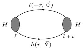
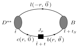
Those two types of correlators are depicted in Figure 1. On each of the two ensembles, we estimate the statistical error from a jackknife procedure.
Refer to caption
Refer to caption
Figure 1: Kinematical configuration of the 2-pt correlators (left) and 3-pt correlators (right) we compute.

4 Masses and energies

We decide to concentrate our effort on the analysis of smeared-smeared 2-pt correlators because the benefit of such a technique has been already clearly observed in a previous work by ETMC [31]. Masses and energies of pseudoscalar Bđ”B and Dđ·D mesons are first extracted from a fit of the form

CP​P​(t,ξ→)=đ’”2​(1)2​EP(1)​(ξ→)​(e−E(1)​(ξ→)​t+e−E(1)​(ξ→)​(T−t)),đ’”2​(1)=⟹H(1)|OPH⁣†| 0⟩formulae-sequencesubscriptđ¶đ‘ƒđ‘ƒđ‘Ąâ†’đœƒsuperscriptđ’”212subscriptsuperscript𝐾1𝑃→𝜃superscript𝑒superscript𝐾1→𝜃𝑡superscript𝑒superscript𝐾1→𝜃𝑇𝑡superscriptđ’”21quantum-operator-productsuperscriptđ»1subscriptsuperscriptđ‘‚đ»â€ đ‘ƒâ€‰0C_{PP}(t,\vec{\theta})=\frac{{\cal Z}^{2\,(1)}}{2E^{(1)}_{P}(\vec{\theta})}\left(e^{-E^{(1)}(\vec{\theta})t}+e^{-E^{(1)}(\vec{\theta})(T-t)}\right),\;\;{\cal Z}^{2\,(1)}=\langle H^{(1)}\,|\,O^{H{\dagger}}_{P}\,|\,0\rangle

in a time range where the contribution from the first excitation is small compared to the statistical error. The stability of the fit is checked by enlarging the time interval and adding a second exponential in the fomula, i.e.:

CP​P​(t,ξ→)=∑i=12đ’”2​(i)2​EP(i)​(ξ→)​(e−E(i)​(ξ→)​t+e−E(i)​(ξ→)​(T−t))subscriptđ¶đ‘ƒđ‘ƒđ‘Ąâ†’đœƒsuperscriptsubscript𝑖12superscriptđ’”2𝑖2subscriptsuperscript𝐾𝑖𝑃→𝜃superscript𝑒superscript𝐾𝑖→𝜃𝑡superscript𝑒superscript𝐾𝑖→𝜃𝑇𝑡C_{PP}(t,\vec{\theta})=\sum_{i=1}^{2}\frac{{\cal Z}^{2\,(i)}}{2E^{(i)}_{P}(\vec{\theta})}\left(e^{-E^{(i)}(\vec{\theta})t}+e^{-E^{(i)}(\vec{\theta})(T-t)}\right)

The last step in the analysis is to measure the effective energy EP≡EP(1)subscript𝐾𝑃subscriptsuperscript𝐾1𝑃E_{P}\equiv E^{(1)}_{P} of the ground state from the ratio

CP​P​(t+1,ξ→)CP​P​(t,ξ→)=cosh⁥(EP​(ξ→))+sinh⁥(EP​(ξ→))​tanh⁥[EP​(ξ→)​(t−T/2)]subscriptđ¶đ‘ƒđ‘ƒđ‘Ą1→𝜃subscriptđ¶đ‘ƒđ‘ƒđ‘Ąâ†’đœƒsubscript𝐾𝑃→𝜃subscript𝐾𝑃→𝜃subscript𝐾𝑃→𝜃𝑡𝑇2\frac{C_{PP}(t+1,\vec{\theta})}{C_{PP}(t,\vec{\theta})}=\cosh(E_{P}(\vec{\theta}))+\sinh(E_{P}(\vec{\theta}))\tanh[E_{P}(\vec{\theta})(t-T/2)]

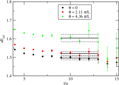
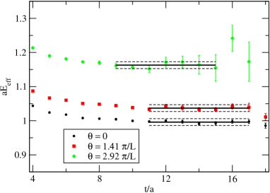
We show in Figure 2 examples of plateaus for ”Bđ”B”-mesons energies at three different momenta.
Refer to caption
Refer to caption
Figure 2: Effective energies of ”Bđ”B”-mesons measured with the ETMC ensemble (ÎČ=3.9đ›œ3.9\beta=3.9, ÎŒsea=ÎŒl=0.0085subscript𝜇seasubscript𝜇𝑙0.0085\mu_{\rm sea}=\mu_{l}=0.0085): ÎŒh=0.3498subscript𝜇ℎ0.3498\mu_{h}=0.3498 (left) and ÎŒh=0.6694subscript𝜇ℎ0.6694\mu_{h}=0.6694 (right).

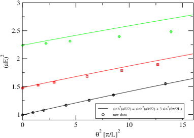
We study the dispersion relation to get an idea of the magnitude of cut-off effects. We display in Figure 3 the Bđ”B meson energies and compare them to the theoretical formula

sinh2⁡[a​E​(ξ)/2]=sinh2⁡[a​M/2]+3​sin2⁡(ξ/2)whereM≡E​(0)formulae-sequencesuperscript2𝑎𝐾𝜃2superscript2𝑎𝑀23superscript2𝜃2where𝑀𝐾0\sinh^{2}[aE(\theta)/2]=\sinh^{2}[aM/2]+3\sin^{2}(\theta/2)\qquad\text{where}\qquad M\equiv E(0) (4.1)
Refer to caption
Figure 3: Comparison of the ”Bđ”B”-mesons energies with the dispersion relation, at the ETMC ensemble (ÎČ=3.9đ›œ3.9\beta=3.9, ÎŒsea=ÎŒl=0.0085subscript𝜇seasubscript𝜇𝑙0.0085\mu_{\rm sea}=\mu_{l}=0.0085). The energy have been rescaled to 1 for the lightest Bđ”B at rest. The black, red and green points correspond to the three Bđ”B masses in increasing order.

The agreement is good at the two lightest heavy masses but really bad at the heaviest one: cut-off effects are pretty large.

Interpolating fields of the 2+superscript22^{+} state are given by the formula O(λ)=ϔΌ​Μ∗(λ)â€‹Ï‡ÂŻcâ€‹ÎłÎŒâ€‹âˆ‡ÎœÏ‡lsuperscript𝑂𝜆subscriptsuperscriptitalic-Ï”absent𝜆𝜇𝜈subscript¯𝜒𝑐subscriptđ›Ÿđœ‡subscript∇𝜈subscript𝜒𝑙O^{(\lambda)}=\epsilon^{*(\lambda)}_{\mu\nu}\bar{\chi}_{c}\gamma_{\mu}\nabla_{\nu}\chi_{l}, λ=±2,±1, 0𝜆plus-or-minus2plus-or-minus1 0\lambda=\pm 2,\,\pm 1,\,0. Actually we choose to use linear combinations of those interpolating fields that read:

{O~(1)=12​(O(+2)+O(−2))=12â€‹Ï‡ÂŻc​(Îł1​∇1−γ2​∇2)​χlO~(2)=O(0)=−16â€‹Ï‡ÂŻc​(Îł1​∇1+Îł2​∇2−2​γ3​∇3)​χlO~(3)=12​(O(+2)−O(−2))=−i2â€‹Ï‡ÂŻc​(Îł1​∇2+Îł2​∇1)​χlO~(4)=12​(O(+1)+O(−1))=i2â€‹Ï‡ÂŻc​(Îł2​∇3+Îł3​∇2)​χlO~(5)=12​(O(+1)−O(−1))=−12â€‹Ï‡ÂŻc​(Îł1​∇3+Îł3​∇1)​χl\left\{\begin{aligned} \tilde{O}^{(1)}&\ =\ \frac{1}{\sqrt{2}}(O^{(+2)}+O^{(-2)})\ =\ \frac{1}{\sqrt{2}}\bar{\chi}_{c}(\gamma_{1}\nabla_{1}-\gamma_{2}\nabla_{2})\chi_{l}\\[8.53581pt] \tilde{O}^{(2)}&\ =O^{(0)}\ =\ -\frac{1}{\sqrt{6}}\bar{\chi}_{c}(\gamma_{1}\nabla_{1}+\gamma_{2}\nabla_{2}-2\gamma_{3}\nabla_{3})\chi_{l}\\[8.53581pt] \tilde{O}^{(3)}&\ =\ \frac{1}{\sqrt{2}}(O^{(+2)}-O^{(-2)})\ =\ -\frac{i}{\sqrt{2}}\bar{\chi}_{c}(\gamma_{1}\nabla_{2}+\gamma_{2}\nabla_{1})\chi_{l}\\[8.53581pt] \tilde{O}^{(4)}&\ =\ \frac{1}{\sqrt{2}}(O^{(+1)}+O^{(-1)})\ =\ \frac{i}{\sqrt{2}}\bar{\chi}_{c}(\gamma_{2}\nabla_{3}+\gamma_{3}\nabla_{2})\chi_{l}\\[8.53581pt] \tilde{O}^{(5)}&\ =\ \frac{1}{\sqrt{2}}(O^{(+1)}-O^{(-1)})\ =\ -\frac{1}{\sqrt{2}}\bar{\chi}_{c}(\gamma_{1}\nabla_{3}+\gamma_{3}\nabla_{1})\chi_{l}\end{aligned}\right.

The two first interpolating fields live in the E𝐾E representation of the Ohsubscript𝑂ℎO_{h} cubic group symmetry of rotations and inversion in a 3-d spatial lattice, while the three last live in the T2subscript𝑇2T_{2} representation of that group [33]. We finally consider the r𝑟r-symmetrized smeared-smeared 2-pt correlators

C2+,E(2)​(t)=12​[⟹∑x→,y→O~S(1)​(y→,t+t~)​O~S†(1)​(x→,t~)⟩+⟹∑x→,y→O~S(2)​(y→,t+t~)​O~S†(2)​(x→,t~)⟩]subscriptsuperscriptđ¶2superscript2𝐾𝑡12delimited-[]delimited-⟚⟩subscriptâ†’đ‘„â†’đ‘Šsubscriptsuperscript~𝑂1𝑆→𝑩𝑡~𝑡subscriptsuperscript~𝑂†absent1đ‘†â†’đ‘„~𝑡delimited-⟚⟩subscriptâ†’đ‘„â†’đ‘Šsubscriptsuperscript~𝑂2𝑆→𝑩𝑡~𝑡subscriptsuperscript~𝑂†absent2đ‘†â†’đ‘„~𝑡C^{(2)}_{2^{+},E}(t)=\frac{1}{2}\left[\langle\sum_{\vec{x},\vec{y}}\tilde{O}^{(1)}_{S}(\vec{y},t+\tilde{t})\tilde{O}^{{\dagger}(1)}_{S}(\vec{x},\tilde{t})\rangle+\langle\sum_{\vec{x},\vec{y}}\tilde{O}^{(2)}_{S}(\vec{y},t+\tilde{t})\tilde{O}^{{\dagger}(2)}_{S}(\vec{x},\tilde{t})\rangle\right] (4.2)

and

C2+,T2(2)(t)=13[⟹∑x→,y→O~S(3)(y→,t+t~)O~S†(3)(x→,t~)⟩+⟹∑x→,y→O~S(4)(y→,t+t~)O~S†(4)(x→,t~)⟩+⟩+⟹∑x→,y→O~S(5)(y→,t+t~)O~S†(5)(x→,t~)⟩]C^{(2)}_{2^{+},T_{2}}(t)=\frac{1}{3}\left[\langle\sum_{\vec{x},\vec{y}}\tilde{O}^{(3)}_{S}(\vec{y},t+\tilde{t})\tilde{O}^{{\dagger}(3)}_{S}(\vec{x},\tilde{t})\rangle+\langle\sum_{\vec{x},\vec{y}}\tilde{O}^{(4)}_{S}(\vec{y},t+\tilde{t})\tilde{O}^{{\dagger}(4)}_{S}(\vec{x},\tilde{t})\rangle+\rangle+\langle\sum_{\vec{x},\vec{y}}\tilde{O}^{(5)}_{S}(\vec{y},t+\tilde{t})\tilde{O}^{{\dagger}(5)}_{S}(\vec{x},\tilde{t})\rangle\right] (4.3)

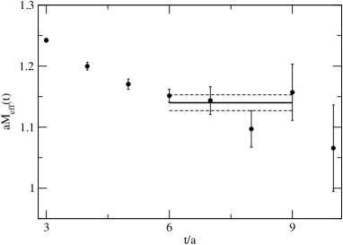
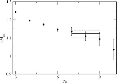
The masses we extract by studying the ratios C2+,E(2)​(t)C2+,E(2)​(t+1)subscriptsuperscriptđ¶2superscript2𝐾𝑡subscriptsuperscriptđ¶2superscript2𝐾𝑡1\frac{C^{(2)}_{2^{+},E}(t)}{C^{(2)}_{2^{+},E}(t+1)} and C2+,T2(2)​(t)C2+,T2(2)​(t+1)subscriptsuperscriptđ¶2superscript2subscript𝑇2𝑡subscriptsuperscriptđ¶2superscript2subscript𝑇2𝑡1\frac{C^{(2)}_{2^{+},T_{2}}(t)}{C^{(2)}_{2^{+},T_{2}}(t+1)} are in principal equal: any discrepancy comes from cut-off effects. We show in Figure 4 that, indeed, lattice artefacts are present.
Refer to caption
Refer to caption
Figure 4: Effective mass of the D2∗subscriptsuperscriptđ·2D^{*}_{2} meson measured with the ETMC ensemble (ÎČ=3.9đ›œ3.9\beta=3.9, ÎŒsea=ÎŒl=0.0085subscript𝜇seasubscript𝜇𝑙0.0085\mu_{\rm sea}=\mu_{l}=0.0085): C2+,E(2)​(t)C2+,E(2)​(t+1)subscriptsuperscriptđ¶2superscript2𝐾𝑡subscriptsuperscriptđ¶2superscript2𝐾𝑡1\frac{C^{(2)}_{2^{+},E}(t)}{C^{(2)}_{2^{+},E}(t+1)} (left) and C2+,T2(2)​(t)C2+,T2(2)​(t+1)subscriptsuperscriptđ¶2superscript2subscript𝑇2𝑡subscriptsuperscriptđ¶2superscript2subscript𝑇2𝑡1\frac{C^{(2)}_{2^{+},T_{2}}(t)}{C^{(2)}_{2^{+},T_{2}}(t+1)} (right).

As parity is broken by Twisted-mass action at finite lattice spacing [23] and the states we consider are not made with quarks of the same flavour doublet, contrary to what is discussed in section 5.2 of [24], the scalar Dđ·D meson can in principle mix with the pseudoscalar Dđ·D meson. We have to build a matrix of correlators {Ci​j​(t)}subscriptđ¶đ‘–đ‘—đ‘Ą\{C_{ij}(t)\} and solve a Generalised Eigenvalue Problem (GEVP) [34] - [36]. We study a 2×2222\times 2 system whose entries correspond to the interpolating fields with Dirac structures Ï‡ÂŻc​γ5​χlsubscript¯𝜒𝑐superscriptđ›Ÿ5subscript𝜒𝑙\bar{\chi}_{c}\gamma^{5}\chi_{l} and Ï‡ÂŻc​χlsubscript¯𝜒𝑐subscript𝜒𝑙\bar{\chi}_{c}\chi_{l}:

Ci​j​(t)=[CÏ‡ÂŻc​γ5​χl;Ï‡ÂŻl​γ5​χc(2)​(t)CÏ‡ÂŻc​γ5​χl;iâ€‹Ï‡ÂŻl​χc(2)​(t)C−iâ€‹Ï‡ÂŻc​χl;Ï‡ÂŻl​γ5​χc(2)​(t)CÏ‡ÂŻc​χl;Ï‡ÂŻl​χc(2)​(t)]subscriptđ¶đ‘–đ‘—đ‘Ądelimited-[]subscriptsuperscriptđ¶2subscript¯𝜒𝑐subscriptđ›Ÿ5subscript𝜒𝑙subscript¯𝜒𝑙subscriptđ›Ÿ5subscript𝜒𝑐𝑡subscriptsuperscriptđ¶2subscript¯𝜒𝑐subscriptđ›Ÿ5subscript𝜒𝑙𝑖subscript¯𝜒𝑙subscript𝜒𝑐𝑡subscriptsuperscriptđ¶2𝑖subscript¯𝜒𝑐subscript𝜒𝑙subscript¯𝜒𝑙subscriptđ›Ÿ5subscript𝜒𝑐𝑡subscriptsuperscriptđ¶2subscript¯𝜒𝑐subscript𝜒𝑙subscript¯𝜒𝑙subscript𝜒𝑐𝑡C_{ij}(t)=\left[\begin{array}[]{ll}C^{(2)}_{\bar{\chi}_{c}\gamma_{5}\chi_{l};\bar{\chi}_{l}\gamma_{5}\chi_{c}}(t)&C^{(2)}_{\bar{\chi}_{c}\gamma_{5}\chi_{l};i\bar{\chi}_{l}\chi_{c}}(t)\\[5.69054pt] C^{(2)}_{-i\bar{\chi}_{c}\chi_{l};\bar{\chi}_{l}\gamma_{5}\chi_{c}}(t)&C^{(2)}_{\bar{\chi}_{c}\chi_{l};\bar{\chi}_{l}\chi_{c}}(t)\end{array}\right]

We solve the system

Ci​j​(t)​vj(n)​(t,t0)=λ(n)​(t,t0)​Ci​j​(t0)​vj(n)​(t,t0)subscriptđ¶đ‘–đ‘—đ‘Ąsubscriptsuperscript𝑣𝑛𝑗𝑡subscript𝑡0superscript𝜆𝑛𝑡subscript𝑡0subscriptđ¶đ‘–đ‘—subscript𝑡0subscriptsuperscript𝑣𝑛𝑗𝑡subscript𝑡0C_{ij}(t)v^{(n)}_{j}(t,t_{0})=\lambda^{(n)}(t,t_{0})C_{ij}(t_{0})v^{(n)}_{j}(t,t_{0}) (4.4)

We set t0=3subscript𝑡03t_{0}=3 (ÎČ=3.9)đ›œ3.9(\beta=3.9) and 5 (ÎČ=4.05)đ›œ4.05(\beta=4.05). λ(n)​(t,t0)superscript𝜆𝑛𝑡subscript𝑡0\lambda^{(n)}(t,t_{0}) and v(n)​(t,t0)superscript𝑣𝑛𝑡subscript𝑡0v^{(n)}(t,t_{0}) are the eigenvalues and eigenvectors of the matrix C−1​(t0)​C​(t)superscriptđ¶1subscript𝑡0đ¶đ‘ĄC^{-1}(t_{0})C(t). The effective mass mD0∗subscript𝑚subscriptsuperscriptđ·0m_{D^{*}_{0}} of the scalar meson is given by:

λ(2)​(t,t0)=cosh⁥[mD0∗​(T/2−t)]cosh⁥[mD0∗​(T/2−t0)]superscript𝜆2𝑡subscript𝑡0subscript𝑚subscriptsuperscriptđ·0𝑇2𝑡subscript𝑚subscriptsuperscriptđ·0𝑇2subscript𝑡0\lambda^{(2)}(t,t_{0})=\frac{\cosh[m_{D^{*}_{0}}(T/2-t)]}{\cosh[m_{D^{*}_{0}}(T/2-t_{0})]} (4.5)

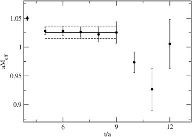
We show in Figure 5 mD0∗subscript𝑚subscriptsuperscriptđ·0m_{D^{*}_{0}} for the ensemble (ÎČ=3.9,ÎŒsea=0.0085formulae-sequenceđ›œ3.9subscript𝜇sea0.0085\beta=3.9,\mu_{\rm sea}=0.0085). The signal is unfortunately quite short, but still acceptable for our qualitative study.
Refer to caption
Figure 5: Effective mass of the D0∗subscriptsuperscriptđ·0D^{*}_{0} meson measured with the ETMC ensemble (ÎČ=3.9đ›œ3.9\beta=3.9, ÎŒsea=ÎŒl=0.0085subscript𝜇seasubscript𝜇𝑙0.0085\mu_{\rm sea}=\mu_{l}=0.0085).

We collect in the Appendix all the masses and energies that we extracted in our analysis. The total error includes the statistical one and the discrepancy of results when we change the time range [tmin,tmax]subscript𝑡minsubscript𝑡max[t_{\rm min},t_{\rm max}] of fits by tmin±1plus-or-minussubscript𝑡min1t_{\rm min}\pm 1 and tmax±1plus-or-minussubscript𝑡max1t_{\rm max}\pm 1, when we take different t0subscript𝑡0t_{0} in the range [3, 6] and, in the case of pseudoscalar Bđ”B mesons, when we perform a 2-states exponential fit.

4.1 đ‘Žđ‘«đŸâˆ—âˆ’đ‘Žđ‘«subscript𝑮subscriptsuperscriptđ‘«bold-∗2subscriptđ‘Žđ‘«\boldsymbol{M_{D^{\ast}_{2}}-M_{D}} and đ‘Žđ‘«đŸŽâˆ—âˆ’đ‘Žđ‘«subscript𝑮subscriptsuperscriptđ‘«bold-∗0subscriptđ‘Žđ‘«\boldsymbol{M_{D^{\ast}_{0}}-M_{D}} in the continuum limit and experiment

In Table 7 in the appendix are given the masses of the D2∗,D0∗subscriptsuperscriptđ·âˆ—2subscriptsuperscriptđ·âˆ—0{D^{\ast}_{2}},{D^{\ast}_{0}} and Dđ·D mesons. It is interesting to perform an extrapolation to the continuum and compare with the experimental data. For the latter we will take the c​s¯𝑐¯𝑠c\bar{s} mesons. It does not change anything for the tensor meson as compared to the non-strange charmed mesons (MD2∗​(2460)−MD≃MD2​s∗​(2573)−MDssimilar-to-or-equalssubscript𝑀subscriptsuperscriptđ·âˆ—22460subscriptđ‘€đ·subscript𝑀subscriptsuperscriptđ·âˆ—2𝑠2573subscript𝑀subscriptđ·đ‘ M_{D^{\ast}_{2}}(2460)-M_{D}\simeq M_{D^{\ast}_{2s}}(2573)-M_{D_{s}}) but for the scalar mesons it does, since the D0​s∗​(2317)subscriptsuperscriptđ·âˆ—0𝑠2317D^{\ast}_{0s}(2317) has a narrow and clear signal which is not the case of the D0∗​(2400)subscriptsuperscriptđ·âˆ—02400D^{\ast}_{0}(2400) whose signal is very broad due to its S-wave decay into Dâ€‹Ï€đ·đœ‹D\pi.

lattice spacing (fm) inverse spacing (GeV) scalar tensor
0.085(3) 2.32(8) 0.58(9) 0.88(7)
0.069(2) 2.85(8) 0.51(5) 0.88(5)
0.0054(2) 3.65(8) 0.51(5)
0.0 infinfimum\inf 0.44(7) 0.88(7) (+15−18)matrix1518\begin{pmatrix}+15\\ -18\end{pmatrix}
Exp. 0.349 0.605
Table 3: Mass differences MD0∗−MDsubscript𝑀subscriptsuperscriptđ·âˆ—0subscriptđ‘€đ·M_{D^{\ast}_{0}}-M_{D} (third column) and MD2∗−MDsubscript𝑀subscriptsuperscriptđ·âˆ—2subscriptđ‘€đ·M_{D^{\ast}_{2}}-M_{D} (fourth column) for ÎČ=3.9đ›œ3.9\beta=3.9 (first line), ÎČ=4.05đ›œ4.05\beta=4.05 (second line) and ÎČ=4.2đ›œ4.2\beta=4.2 (third line), the latter being for the moment restricted to MD0∗−MDsubscript𝑀subscriptsuperscriptđ·âˆ—0subscriptđ‘€đ·M_{D^{\ast}_{0}}-M_{D}. We use the lattice spacings reported in Table 2. The extrapolation to vanishing lattice spacing is in the fourth line and the experimental data MD0​s∗​(2317)−MDssubscript𝑀subscriptsuperscriptđ·âˆ—0𝑠2317subscript𝑀subscriptđ·đ‘ M_{D^{\ast}_{0s}}(2317)-M_{D_{s}} and MD2​s∗​(2573)−MDssubscript𝑀subscriptsuperscriptđ·âˆ—2𝑠2573subscript𝑀subscriptđ·đ‘ M_{D^{\ast}_{2s}}(2573)-M_{D_{s}} are in the fifth line. The errors combine in quadrature the errors on the masses in lattice units and on the lattice spacing. The fitting windows are reported in table 7. The dependence of the value extrapolated to continuum strongly depends on the lattice spacing. Our uncertainty does not incorporate the systematic one due to the choice of the fitting windows. Our mass differences extrapolated to the continuum are above experiment.

We perform the extrapolation to the continuum limit and compute the error using jackknife. We show our results in Table 3. We see that the agreement with experiment is not so good but the errors are large. For the moment we cannot say much, except that the future will tell whether this issue comes mainly from statistical fluctuations or whether the lattice regularization is in cause. A similar conclusion was made recently in a lattice study with Nf=2+1+1subscriptNf211{\rm N_{f}}=2+1+1 dynamical quarks regularised by TmQCD [39]. Also, we have not considered yet the possible effect of the opening of the decay channel D0∗→D​π→subscriptsuperscriptđ·0đ·đœ‹D^{*}_{0}\to D\pi S𝑆S-wave state as proposed in [40].

5 đ‘©đ‘©\boldsymbol{B} decay to the scalar đ‘«đŸŽâˆ—subscriptsuperscriptđ‘«0\boldsymbol{D^{*}_{0}} charmed meson

In this section we will restrict to the zero recoil kinematics, in other words the initial Bđ”B meson is taken at rest. We restrict ourselves to this simpler case because the momentum dependance of the B→D0âˆ—â†’đ”subscriptsuperscriptđ·0B\to D^{*}_{0} decay is very difficult to study on the lattice (3-pt correlators are very noisy) and we cannot yet say anything significant about it, but also because the non vanishing of the zero recoil amplitude is of utmost phenomenological relevance : in the infinite mass limit, the B→D0âˆ—â†’đ”subscriptsuperscriptđ·0B\to D^{*}_{0} amplitude vanishes at zero recoil [13]. This forbids the decay into a S-wave between the lepton pair and the D0∗subscriptsuperscriptđ·0D^{*}_{0} since an S-wave clearly does not vanish at zero recoil. The S-wave is a major contribution to these decays since their available phase space is rather small, and higher waves are suppresed by the so-called centrifugal barreer effect. With finite heavy quark masses we will show that the zero recoil amplitude does not vanish, there is a non vanishing S-wave and this may change drastically the ratio between Γ​(B→D2∗)Î“â†’đ”subscriptsuperscriptđ·2\Gamma(B\to D^{*}_{2}) and Γ​(B→D0∗)Î“â†’đ”subscriptsuperscriptđ·0\Gamma(B\to D^{*}_{0}) since the B→D2âˆ—â†’đ”subscriptsuperscriptđ·2B\to D^{*}_{2} decay amplitude does vanish at zero recoil whether the mass of the c𝑐c and b𝑏b is taken infinite or finite, thus implying only a D-wave decay. The possible importance of a non vanishing zero recoil amplitude was stressed in [37] where the authors estimated subleading corrections to the infinite mass limit : although subleading in the Λ/mc,bΛsubscript𝑚𝑐𝑏\Lambda/m_{c,b} expansion, the S-wave may not be negligible. Our computation confirms this conclusion as shall be seen.

5.1 Computation of the amplitude ratio (đ‘©â†’đ‘«đŸŽâˆ—)bold-â†’đ‘©subscriptsuperscriptđ‘«0\boldsymbol{(B\to D^{*}_{0}}) over (đ‘©â†’đ‘«)bold-â†’đ‘©đ‘«\boldsymbol{(B\to D)} at zero recoil

We will compute the ratio of amplitudes A​(B→D0∗)/A​(B→D)đŽâ†’đ”subscriptsuperscriptđ·0đŽâ†’đ”đ·A(B\to D^{*}_{0})/A(B\to D). We take A​(B→D)đŽâ†’đ”đ·A(B\to D) as a benchmark since it is experimentally fairly well known, and Dđ·D being a J=0đœ0J=0 state as D0∗subscriptsuperscriptđ·0D^{*}_{0}, it is expected that the momentum dependence of these decays will be rather similar. We recall some formulae neglecting for the moment the D−D0âˆ—đ·subscriptsuperscriptđ·0D-D^{*}_{0} mixing due to the parity violation at finite lattice spacing when using twisted mass quarks. The matrix elements ⟹B|V0|D⟩quantum-operator-productđ”subscript𝑉0đ·\langle B|V_{0}|D\rangle and ⟹B|A0|D0∗⟩quantum-operator-productđ”subscript𝐮0subscriptsuperscriptđ·0\langle B|A_{0}|D^{*}_{0}\rangle are given by the following ratio

⟹B|O|Hc⟩=CBOHc(3)​(tp,t,ts)​ZHc/ZB​ZOCHc(2)​(t−ts)​exp⁥(−EB​(tp−t))/(2​EB),quantum-operator-productđ”đ‘‚subscriptđ»đ‘subscriptsuperscriptđ¶3subscriptBOHcsubscript𝑡𝑝𝑡subscript𝑡𝑠subscript𝑍subscriptđ»đ‘subscriptđ‘đ”subscript𝑍𝑂subscriptsuperscriptđ¶2subscriptđ»đ‘đ‘Ąsubscript𝑡𝑠subscriptđžđ”subscript𝑡𝑝𝑡2subscriptđžđ”\displaystyle\langle B|O|H_{c}\rangle=\frac{C^{(3)}_{\rm BOH_{c}}(t_{p},t,t_{s})\sqrt{Z_{H_{c}}/Z_{B}}Z_{O}}{C^{(2)}_{H_{c}}(t-t_{s})\exp(-E_{B}\,(t_{p}-t))/(2E_{B})}\,, (5.1)

where ts<t<tpsubscript𝑡𝑠𝑡subscript𝑡𝑝t_{s}<t<t_{p} are respectively the source, current and sink times (cf Fig 1).

Z0=ZV​(ZA)subscript𝑍0subscript𝑍𝑉subscript𝑍𝐮Z_{0}=Z_{V}(Z_{A}) when Hc=D​(D0∗)subscriptđ»đ‘đ·subscriptsuperscriptđ·0H_{c}=D(D^{*}_{0}). ZHcsubscript𝑍subscriptđ»đ‘Z_{H_{c}} and ZBsubscriptđ‘đ”Z_{B} are defined from the fit of the 2-pt correlators of the Hcsubscriptđ»đ‘H_{c} and Bđ”B mesons, assuming we are far enough from the center of the lattice to be allowed to neglect the backward exponential in time while the contribution of excited states is small.

CB(2)​(t,ξ→)=ZB2​EB​(ξ→)​exp⁥(−EB​(ξ→))​t;CHc(2)​(t,0)=ZHc2​MHc​exp⁥(−MHc​t).formulae-sequencesubscriptsuperscriptđ¶2đ”đ‘Ąâ†’đœƒsubscriptđ‘đ”2subscriptđžđ”â†’đœƒsubscriptđžđ”â†’đœƒđ‘Ąsubscriptsuperscriptđ¶2subscriptđ»đ‘đ‘Ą0subscript𝑍subscriptđ»đ‘2subscript𝑀subscriptđ»đ‘subscript𝑀subscriptđ»đ‘đ‘Ą\displaystyle C^{(2)}_{B}(t,\vec{\theta})=\frac{Z_{B}}{2E_{B}(\vec{\theta})}\exp(-E_{B}(\vec{\theta}))t;\qquad C^{(2)}_{H_{c}}(t,0)=\frac{Z_{H_{c}}}{2M_{H_{c}}}\exp\left(-M_{H_{c}}t\right)\,. (5.2)

Then we compute

⟹B|A0|D0∗⟩⟚B|V0|D⟩=CBA0​D0∗(3)​(tp,t,ts)​CD(2)​(t−ts)​ZA​ZD0∗CBV0​D(3)​(tp,t,ts)​CD0∗(2)​(t−ts)​ZV​ZD.quantum-operator-productđ”subscript𝐮0subscriptsuperscriptđ·0quantum-operator-productđ”subscript𝑉0đ·subscriptsuperscriptđ¶3subscriptBA0subscriptsuperscriptD0subscript𝑡𝑝𝑡subscript𝑡𝑠subscriptsuperscriptđ¶2đ·đ‘Ąsubscript𝑡𝑠subscript𝑍𝐮subscript𝑍subscriptsuperscriptđ·0subscriptsuperscriptđ¶3subscriptBV0Dsubscript𝑡𝑝𝑡subscript𝑡𝑠subscriptsuperscriptđ¶2subscriptsuperscriptđ·0𝑡subscript𝑡𝑠subscript𝑍𝑉subscriptđ‘đ·\displaystyle\frac{\langle B|A_{0}|D^{*}_{0}\rangle}{\langle B|V_{0}|D\rangle}=\frac{C^{(3)}_{\rm BA_{0}D^{*}_{0}}(t_{p},t,t_{s})C^{(2)}_{D}(t-t_{s})Z_{A}\sqrt{Z_{D^{*}_{0}}}}{C^{(3)}_{\rm BV_{0}D}(t_{p},t,t_{s})C^{(2)}_{D^{*}_{0}}(t-t_{s})Z_{V}\sqrt{Z_{D}}}\,. (5.3)
v(1)superscript𝑣1v^{(1)} v(2)superscript𝑣2v^{(2)}
0.97 0.28  i
0.22 i 0.96
Table 4: Values of the approximately orthonormalised eigenvectors v(1)superscript𝑣1v^{(1)} and v(2)superscript𝑣2v^{(2)}, eq. (4.5), for ÎČ=3.9đ›œ3.9\beta=3.9, t0=ts=3subscript𝑡0subscript𝑡𝑠3t_{0}=t_{s}=3, t=7𝑡7t=7 and tp=14subscript𝑡𝑝14t_{p}=14. v(1)​v(2)⁣†=0.07​isuperscript𝑣1superscript𝑣2†0.07𝑖v^{(1)}v^{(2)\dagger}=0.07\,i, rather small as expected in eq 5.4.

5.2 Taking into account the scalar-pseudoscalar mixing

In section 4 we have detailed the Generalised Eigenvalue method. As explained there and in section 3, we restrict ourselves to a 2×2222\times 2 matrix of smeared and stochastic 2-pt correlators. The largest (smallest) eigenvalue λ(1)superscript𝜆1\lambda^{(1)} (λ(2)superscript𝜆2\lambda^{(2)} ) will be related to the mass of the Dđ·D (D0∗subscriptsuperscriptđ·0D^{*}_{0}) state. The corresponding eigenvectors give the linear combination of Ï‡ÂŻc​γ5​χlsubscript¯𝜒𝑐subscriptđ›Ÿ5subscript𝜒𝑙\bar{\chi}_{c}\gamma_{5}\chi_{l} and Ï‡ÂŻc​χlsubscript¯𝜒𝑐subscript𝜒𝑙\bar{\chi}_{c}\chi_{l} interpolating fields that have the largest coupling to the D​(D0∗)đ·subscriptsuperscriptđ·0D(D^{*}_{0}) state. The eigenvectors turn out to be not far from orthogonal

v(1)​v(2)⁣†=∑k=1,2vk(1)​vk(2)⁣⋆=0.07​i≃0,superscript𝑣1superscript𝑣2†subscript𝑘12subscriptsuperscript𝑣1𝑘subscriptsuperscript𝑣2⋆𝑘0.07𝑖similar-to-or-equals0\displaystyle v^{(1)}v^{(2)\dagger}=\sum_{k=1,2}v^{(1)}_{k}v^{(2)\star}_{k}=0.07i\simeq 0\,, (5.4)

as seen for example in table 4. One might say that 0.07 is not so small but this is not surprising, since there are other states in which the B might decay than only the ground state scalar and pseudoscalar that we consider in our analysis. We can thus to a fair approximation orthonormalise the eigenvectors so that

v(i)​v(j)⁣†≃ήi,j,similar-to-or-equalssuperscript𝑣𝑖superscript𝑣𝑗†subscript𝛿𝑖𝑗\displaystyle v^{(i)}v^{(j)\dagger}\simeq\delta_{i,j}\,, (5.5)

without changing the eigenvalues, since in eq (4.4) the same factor multiplies both sides of the equation. Thus, we define the 2-pt correlator of D0∗subscriptsuperscriptđ·0D^{*}_{0} meson by

λ(2)​(t−ts,t0)​∑i,j=12vi(2)⁣†​(t−ts,t0)​Ci​j(2)​(t0)​vj(2)​(t−ts,t0)superscript𝜆2𝑡subscript𝑡𝑠subscript𝑡0superscriptsubscript𝑖𝑗12subscriptsuperscript𝑣2†𝑖𝑡subscript𝑡𝑠subscript𝑡0subscriptsuperscriptđ¶2𝑖𝑗subscript𝑡0subscriptsuperscript𝑣2𝑗𝑡subscript𝑡𝑠subscript𝑡0\displaystyle\lambda^{(2)}(t-t_{s},t_{0})\sum_{i,j=1}^{2}v^{(2)\,\dagger}_{i}(t-t_{s},t_{0})C^{(2)}_{ij}(t_{0})v^{(2)}_{j}(t-t_{s},t_{0}) =\displaystyle= ∑i,j=12vi(2)⁣†​(t−ts,t0)​Ci​j(2)​(t−ts)​vj(2)​(t−ts,t0),superscriptsubscript𝑖𝑗12subscriptsuperscript𝑣2†𝑖𝑡subscript𝑡𝑠subscript𝑡0subscriptsuperscriptđ¶2𝑖𝑗𝑡subscript𝑡𝑠subscriptsuperscript𝑣2𝑗𝑡subscript𝑡𝑠subscript𝑡0\displaystyle\sum_{i,j=1}^{2}v^{(2)\,\dagger}_{i}(t-t_{s},t_{0})C^{(2)}_{ij}(t-t_{s})v^{(2)}_{j}(t-t_{s},t_{0})\,,
λ(1)​(t−ts,t0)​∑i,j=12vi(1)⁣†​(t−ts,t0)​Ci​j(2)​(t0)​vj(1)​(t−ts,t0)superscript𝜆1𝑡subscript𝑡𝑠subscript𝑡0superscriptsubscript𝑖𝑗12subscriptsuperscript𝑣1†𝑖𝑡subscript𝑡𝑠subscript𝑡0subscriptsuperscriptđ¶2𝑖𝑗subscript𝑡0subscriptsuperscript𝑣1𝑗𝑡subscript𝑡𝑠subscript𝑡0\displaystyle\lambda^{(1)}(t-t_{s},t_{0})\sum_{i,j=1}^{2}v^{(1)\,\dagger}_{i}(t-t_{s},t_{0})C^{(2)}_{ij}(t_{0})v^{(1)}_{j}(t-t_{s},t_{0}) =\displaystyle= ∑i,j=12vi(1)⁣†​(t−ts,t0)​Ci​j(2)​(t−ts)​vj(1)​(t−ts,t0),superscriptsubscript𝑖𝑗12subscriptsuperscript𝑣1†𝑖𝑡subscript𝑡𝑠subscript𝑡0subscriptsuperscriptđ¶2𝑖𝑗𝑡subscript𝑡𝑠subscriptsuperscript𝑣1𝑗𝑡subscript𝑡𝑠subscript𝑡0\displaystyle\sum_{i,j=1}^{2}v^{(1)\,\dagger}_{i}(t-t_{s},t_{0})C^{(2)}_{ij}(t-t_{s})v^{(1)}_{j}(t-t_{s},t_{0})\,, (5.6)

where we fit with

λ(2)​(t−ts,t0)superscript𝜆2𝑡subscript𝑡𝑠subscript𝑡0\displaystyle\lambda^{(2)}(t-t_{s},t_{0}) =\displaystyle= exp⁥(−MD0∗​(t−ts−t0))λ(1)​(t−ts,t0)=exp⁥(−MD​(t−ts−t0))subscript𝑀subscriptsuperscriptđ·0𝑡subscript𝑡𝑠subscript𝑡0superscript𝜆1𝑡subscript𝑡𝑠subscript𝑡0subscriptđ‘€đ·đ‘Ąsubscript𝑡𝑠subscript𝑡0\displaystyle\exp\left(-M_{D^{*}_{0}}(t-t_{s}-t_{0})\right)\quad\lambda^{(1)}(t-t_{s},t_{0})=\exp\left(-M_{D}(t-t_{s}-t_{0})\right) (5.7)

since λ(i)​(t0,t0)=1superscript𝜆𝑖subscript𝑡0subscript𝑡01\lambda^{(i)}(t_{0},t_{0})=1 from Eq. (5.2). We define Z2(1)superscriptsubscript𝑍21Z_{2}^{(1)} and Z2(2)superscriptsubscript𝑍22Z_{2}^{(2)} from

vi(2)⁣†​(t−ts,t0)​Ci​j(2)​(t−ts)​vj(2)​(t−ts,t0)subscriptsuperscript𝑣2†𝑖𝑡subscript𝑡𝑠subscript𝑡0subscriptsuperscriptđ¶2𝑖𝑗𝑡subscript𝑡𝑠subscriptsuperscript𝑣2𝑗𝑡subscript𝑡𝑠subscript𝑡0\displaystyle v^{(2)\,\dagger}_{i}(t-t_{s},t_{0})C^{(2)}_{ij}(t-t_{s})v^{(2)}_{j}(t-t_{s},t_{0}) =\displaystyle= Z2(2)2​MD0∗​exp⁥(−MD0∗​(t−ts)),superscriptsubscript𝑍222subscript𝑀subscriptsuperscriptđ·0subscript𝑀subscriptsuperscriptđ·0𝑡subscript𝑡𝑠\displaystyle\frac{Z_{2}^{(2)}}{2M_{D^{*}_{0}}}\exp\left(-M_{D^{*}_{0}}(t-t_{s})\right)\,, (5.8)
vi(1)⁣†​(t−ts,t0)​Ci​j(2)​(t−ts)​vj(1)​(t−ts,t0)subscriptsuperscript𝑣1†𝑖𝑡subscript𝑡𝑠subscript𝑡0subscriptsuperscriptđ¶2𝑖𝑗𝑡subscript𝑡𝑠subscriptsuperscript𝑣1𝑗𝑡subscript𝑡𝑠subscript𝑡0\displaystyle v^{(1)\,\dagger}_{i}(t-t_{s},t_{0})C^{(2)}_{ij}(t-t_{s})v^{(1)}_{j}(t-t_{s},t_{0}) =\displaystyle= Z1(1)2​MD0∗​exp⁥(−MD​(t−ts)),superscriptsubscript𝑍112subscript𝑀subscriptsuperscriptđ·0subscriptđ‘€đ·đ‘Ąsubscript𝑡𝑠\displaystyle\frac{Z_{1}^{(1)}}{2M_{D^{*}_{0}}}\exp\left(-M_{D}(t-t_{s})\right)\,,

In Eq. (5.1) we see that the factors Zisubscript𝑍𝑖Z_{i} appear only via their square root.

5.2.1 Symmetry properties of the matrix elements

In the continuum it is obvious by parity conservation that

⟹B|A0|D⟩=⟹B|V0|D0∗⟩=0quantum-operator-productđ”subscript𝐮0đ·quantum-operator-productđ”subscript𝑉0subscriptsuperscriptđ·00\displaystyle\langle B|A_{0}|D\rangle=\langle B|V_{0}|D^{*}_{0}\rangle=0 (5.9)

However parity is not conserved by the twisted mass quark action at finite lattice spacing. But this action has an exact symmetry [23], the flavour-parity

ℛ5spâ‰Ąđ’«âŠ—(ÎŒl,ÎŒc,ÎŒb↝−Όl,−Όc,−Όb)\displaystyle{\mathscr{R}}^{\rm sp}_{5}\equiv{\mathscr{P}}\otimes\left({\mu_{l},\mu_{c},\mu_{b}\leadsto-\mu_{l},-\mu_{c},-\mu_{b}}\right) (5.10)

where đ’«đ’«\mathscr{P} is the spatial parity, and ÎŒl,ÎŒc,ÎŒbsubscript𝜇𝑙subscript𝜇𝑐subscript𝜇𝑏\mu_{l},\mu_{c},\mu_{b} are the twisted mass terms for the light, charm and beauty quarks. We assume we are at maximal twist (vanishing of mPCACsubscript𝑚PCACm_{\rm PCAC}). Therefore if we use

Ci,j,k(3)​sym​(tp,t,ts)≡(1+ℛ5sp)​Ci,j,k(3)​(tp,t,ts)subscriptsuperscriptđ¶3sym𝑖𝑗𝑘subscript𝑡𝑝𝑡subscript𝑡𝑠1subscriptsuperscriptℛsp5subscriptsuperscriptđ¶3𝑖𝑗𝑘subscript𝑡𝑝𝑡subscript𝑡𝑠\displaystyle C^{(3)\,\text{sym}}_{i,j,k}(t_{p},t,t_{s})\ \equiv\ \left(1+{\mathscr{R}}^{\rm sp}_{5}\right)\,C^{(3)}_{i,j,k}(t_{p},t,t_{s}) (5.11)

we get the validity of eq. (5.9) also for finite lattice spacing. This symmetrisation will be assumed in the following.

5.2.2 GEVP on the 3 pt correlators

In this section we assume ts<t<tpsubscript𝑡𝑠𝑡subscript𝑡𝑝t_{s}<t<t_{p} and t0≀t−tssubscript𝑡0𝑡subscript𝑡𝑠t_{0}\leq t-t_{s}. Starting from the 3-pt correlators CB​A0​(V0)​Oi(3)​(tp,t,ts)=âŸšÏ‡ÂŻb​γ5​χl​(tp)​A0​(V0)​(t)​Oi​(Ï‡ÂŻc,χl,ts)⟩subscriptsuperscriptđ¶3đ”subscript𝐮0subscript𝑉0subscript𝑂𝑖subscript𝑡𝑝𝑡subscript𝑡𝑠delimited-⟚⟩subscript¯𝜒𝑏subscriptđ›Ÿ5subscript𝜒𝑙subscript𝑡𝑝subscript𝐮0subscript𝑉0𝑡subscript𝑂𝑖subscript¯𝜒𝑐subscript𝜒𝑙subscript𝑡𝑠C^{(3)}_{BA_{0}(V_{0})O_{i}}(t_{p},t,t_{s})=\langle\bar{\chi}_{b}\gamma_{5}\chi_{l}(t_{p})A_{0}(V_{0})(t)O_{i}(\bar{\chi}_{c},\chi_{l},t_{s})\rangle, Oi​(Ï‡ÂŻc,χl)≡{Ï‡ÂŻc​γ5​χl,Ï‡ÂŻc​χl}subscript𝑂𝑖subscript¯𝜒𝑐subscript𝜒𝑙subscript¯𝜒𝑐subscriptđ›Ÿ5subscript𝜒𝑙subscript¯𝜒𝑐subscript𝜒𝑙O_{i}(\bar{\chi}_{c},\chi_{l})\equiv\{\bar{\chi}_{c}\gamma_{5}\chi_{l},\,\bar{\chi}_{c}\chi_{l}\} and following the authors [38] in their way of extracting the decay constant fBsubscriptđ‘“đ”f_{B}, we consider the projected 3-pt correlators

CB​A0​D0∗(3)⁣â€Č​(tp,t,ts)subscriptsuperscriptđ¶3â€Čđ”subscript𝐮0subscriptsuperscriptđ·0subscript𝑡𝑝𝑡subscript𝑡𝑠\displaystyle C^{(3)\prime}_{BA_{0}D^{*}_{0}}(t_{p},t,t_{s}) =\displaystyle= âŸšÏ‡ÂŻb​γ5​χl​(tp)​A0​(t)â€‹Ï‡ÂŻc​χl​(ts)​vÏ‡ÂŻc​χl(2)​(t−ts,t0)⟩vi†(2)​(t−ts,t0)​Ci​j(2)​(t−ts)​vj(2)​(t−ts,t0)delimited-⟚⟩subscript¯𝜒𝑏subscriptđ›Ÿ5subscript𝜒𝑙subscript𝑡𝑝subscript𝐮0𝑡subscript¯𝜒𝑐subscript𝜒𝑙subscript𝑡𝑠subscriptsuperscript𝑣2subscript¯𝜒𝑐subscript𝜒𝑙𝑡subscript𝑡𝑠subscript𝑡0subscriptsuperscript𝑣†absent2𝑖𝑡subscript𝑡𝑠subscript𝑡0subscriptsuperscriptđ¶2𝑖𝑗𝑡subscript𝑡𝑠subscriptsuperscript𝑣2𝑗𝑡subscript𝑡𝑠subscript𝑡0\displaystyle\frac{\langle\bar{\chi}_{b}\gamma_{5}\chi_{l}(t_{p})A_{0}(t)\bar{\chi}_{c}\chi_{l}(t_{s})v^{(2)}_{\bar{\chi}_{c}\chi_{l}}(t-t_{s},t_{0})\rangle}{\sqrt{v^{{\dagger}(2)}_{i}(t-t_{s},t_{0})C^{(2)}_{ij}(t-t_{s})v^{(2)}_{j}(t-t_{s},t_{0})}}
×\displaystyle\times (λ(2)​(t0+a,t0)λ(2)​(t0+2​a,t0))(t−ts)/2​a​2​EB​e(tp−t)​EBZB​2​mD0∗,superscriptsuperscript𝜆2subscript𝑡0𝑎subscript𝑡0superscript𝜆2subscript𝑡02𝑎subscript𝑡0𝑡subscript𝑡𝑠2𝑎2subscriptđžđ”superscript𝑒subscript𝑡𝑝𝑡subscriptđžđ”subscriptđ‘đ”2subscript𝑚subscriptsuperscriptđ·0\displaystyle\left(\frac{\lambda^{(2)}(t_{0}+a,t_{0})}{\lambda^{(2)}(t_{0}+2a,t_{0})}\right)^{(t-t_{s})/2a}\frac{2E_{B}e^{(t_{p}-t)E_{B}}}{\sqrt{Z_{B}}}\sqrt{2m_{D^{*}_{0}}},
CB​V0​D(3)⁣â€Č​(tp,t,ts)subscriptsuperscriptđ¶3â€Čđ”subscript𝑉0đ·subscript𝑡𝑝𝑡subscript𝑡𝑠\displaystyle C^{(3)\prime}_{BV_{0}D}(t_{p},t,t_{s}) =\displaystyle= âŸšÏ‡ÂŻb​γ5​χl​(tp)​V0​(t)â€‹Ï‡ÂŻc​γ5​χl​(ts)​vÏ‡ÂŻc​γ5​χl(1)​(t−ts,t0)⟩vi†(1)​(t−ts,t0)​Ci​j(2)​(t−ts)​vj(1)​(t−ts,t0)delimited-⟚⟩subscript¯𝜒𝑏subscriptđ›Ÿ5subscript𝜒𝑙subscript𝑡𝑝subscript𝑉0𝑡subscript¯𝜒𝑐subscriptđ›Ÿ5subscript𝜒𝑙subscript𝑡𝑠subscriptsuperscript𝑣1subscript¯𝜒𝑐subscriptđ›Ÿ5subscript𝜒𝑙𝑡subscript𝑡𝑠subscript𝑡0subscriptsuperscript𝑣†absent1𝑖𝑡subscript𝑡𝑠subscript𝑡0subscriptsuperscriptđ¶2𝑖𝑗𝑡subscript𝑡𝑠subscriptsuperscript𝑣1𝑗𝑡subscript𝑡𝑠subscript𝑡0\displaystyle\frac{\langle\bar{\chi}_{b}\gamma_{5}\chi_{l}(t_{p})V_{0}(t)\bar{\chi}_{c}\gamma_{5}\chi_{l}(t_{s})v^{(1)}_{\bar{\chi}_{c}\gamma_{5}\chi_{l}}(t-t_{s},t_{0})\rangle}{\sqrt{v^{{\dagger}(1)}_{i}(t-t_{s},t_{0})C^{(2)}_{ij}(t-t_{s})v^{(1)}_{j}(t-t_{s},t_{0})}} (5.12)
×\displaystyle\times (λ(1)​(t0+a,t0)λ(1)​(t0+2​a,t0))(t−ts)/2​a​2​EB​e(tp−t)​EBZB​2​mD.superscriptsuperscript𝜆1subscript𝑡0𝑎subscript𝑡0superscript𝜆1subscript𝑡02𝑎subscript𝑡0𝑡subscript𝑡𝑠2𝑎2subscriptđžđ”superscript𝑒subscript𝑡𝑝𝑡subscriptđžđ”subscriptđ‘đ”2subscriptđ‘šđ·\displaystyle\left(\frac{\lambda^{(1)}(t_{0}+a,t_{0})}{\lambda^{(1)}(t_{0}+2a,t_{0})}\right)^{(t-t_{s})/2a}\frac{2E_{B}e^{(t_{p}-t)E_{B}}}{\sqrt{Z_{B}}}\sqrt{2m_{D}}.

We remind that the normalisation factor Z2(2)subscriptsuperscript𝑍22Z^{(2)}_{2} cancels between âŸšÏ‡ÂŻb​γ5​χl​(tp)​A0​(V0)​(t)â€‹Ï‡ÂŻc​(Îł5)​χl​(ts)⟩delimited-⟚⟩subscript¯𝜒𝑏subscriptđ›Ÿ5subscript𝜒𝑙subscript𝑡𝑝subscript𝐮0subscript𝑉0𝑡subscript¯𝜒𝑐subscriptđ›Ÿ5subscript𝜒𝑙subscript𝑡𝑠\langle\bar{\chi}_{b}\gamma_{5}\chi_{l}(t_{p})A_{0}(V_{0})(t)\bar{\chi}_{c}(\gamma_{5})\chi_{l}(t_{s})\rangle and
vi†(2​(1))​(t−ts,t0)​Ci​j(2)​(t−ts)​vj(2​(1))​(t−ts,t0)subscriptsuperscript𝑣†absent21𝑖𝑡subscript𝑡𝑠subscript𝑡0subscriptsuperscriptđ¶2𝑖𝑗𝑡subscript𝑡𝑠subscriptsuperscript𝑣21𝑗𝑡subscript𝑡𝑠subscript𝑡0\sqrt{v^{{\dagger}(2(1))}_{i}(t-t_{s},t_{0})C^{(2)}_{ij}(t-t_{s})v^{(2(1))}_{j}(t-t_{s},t_{0})} while the factor (λ(2​(1))​(t0+a,t0)λ(2​(1))​(t0+2​a,t0))(t−ts)/2​a∌e−ED0∗​(D)​(t−ts)/2​asimilar-tosuperscriptsuperscript𝜆21subscript𝑡0𝑎subscript𝑡0superscript𝜆21subscript𝑡02𝑎subscript𝑡0𝑡subscript𝑡𝑠2𝑎superscript𝑒subscript𝐾subscriptsuperscriptđ·0đ·đ‘Ąsubscript𝑡𝑠2𝑎\left(\frac{\lambda^{(2(1))}(t_{0}+a,t_{0})}{\lambda^{(2(1))}(t_{0}+2a,t_{0})}\right)^{(t-t_{s})/2a}\sim e^{-E_{D^{*}_{0}(D)}(t-t_{s})/2a} compensates the residual time exponential dependence. We do not take into account the contributions ∝vÏ‡ÂŻc​γ5​χl(2)​(t−ts,t0)proportional-toabsentsuperscriptsubscript𝑣subscript¯𝜒𝑐subscriptđ›Ÿ5subscript𝜒𝑙2𝑡subscript𝑡𝑠subscript𝑡0\propto\,v_{\bar{\chi}_{c}\gamma_{5}\chi_{l}}^{(2)}(t-t_{s},t_{0}) and vÏ‡ÂŻc​χl(1)​(t−ts,t0)superscriptsubscript𝑣subscript¯𝜒𝑐subscript𝜒𝑙1𝑡subscript𝑡𝑠subscript𝑡0v_{\bar{\chi}_{c}\chi_{l}}^{(1)}(t-t_{s},t_{0}) to the projected correlators ∑iâŸšÏ‡ÂŻb​γ5​χl​(tp)​A0​(V0)​(t)​Oi​(Ï‡ÂŻc,χl,ts)​vi(2​(1))​(t−ts,t0)⟩subscript𝑖delimited-⟚⟩subscript¯𝜒𝑏subscriptđ›Ÿ5subscript𝜒𝑙subscript𝑡𝑝subscript𝐮0subscript𝑉0𝑡subscript𝑂𝑖subscript¯𝜒𝑐subscript𝜒𝑙subscript𝑡𝑠subscriptsuperscript𝑣21𝑖𝑡subscript𝑡𝑠subscript𝑡0\sum_{i}\langle\bar{\chi}_{b}\gamma_{5}\chi_{l}(t_{p})A_{0}(V_{0})(t)O_{i}(\bar{\chi}_{c},\chi_{l},t_{s})v^{(2(1))}_{i}(t-t_{s},t_{0})\rangle because the B meson goes through operator A0subscript𝐮0A_{0} (V0subscript𝑉0V_{0}) only to a pure scalar (pseudoscalar) state.

The ratio in eq. 5.3 becomes

⟹B|A0|D0∗⟩⟚B|V0|D⟩quantum-operator-productđ”subscript𝐮0subscriptsuperscriptđ·0quantum-operator-productđ”subscript𝑉0đ·\displaystyle\frac{\langle B|A_{0}|D^{*}_{0}\rangle}{\langle B|V_{0}|D\rangle} ≃similar-to-or-equals\displaystyle\simeq CBA0​D0∗(3)⁣â€Č​(tp,t,ts)CBV0​D(3)⁣â€Č​(tp,t,ts)×ZAZVsubscriptsuperscriptđ¶3â€ČsubscriptBA0subscriptsuperscriptD0subscript𝑡𝑝𝑡subscript𝑡𝑠subscriptsuperscriptđ¶3â€ČsubscriptBV0Dsubscript𝑡𝑝𝑡subscript𝑡𝑠subscript𝑍𝐮subscript𝑍𝑉\displaystyle\frac{C^{(3)\prime}_{\rm BA_{0}D^{*}_{0}}(t_{p},t,t_{s})}{C^{(3)\prime}_{\rm BV_{0}D}(t_{p},t,t_{s})}\times\frac{Z_{A}}{Z_{V}} (5.13)

using eq (5.7)

Of course the ratio of branching fractions has to take into account the difference in phase space. However, we ignore totally the dependence of the amplitude on the recoil, having only estimated the zero recoil contribution. Therefore, we will for the moment neglect the phase space dependence. We collect the results of eq. 5.13 in Table 5 and show plateaus in Figure 6.
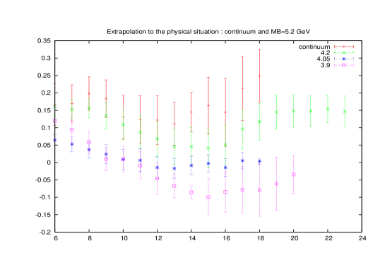
Refer to caption
Figure 6: The ratio in eq. (5.13) once symmetrised according to Eq. (5.11) extrapoleted from the three b𝑏b quark masses to the physical B mass : 5.2 GeV, linearly in 1/MB1subscriptđ‘€đ”1/M_{B}. We have used data from ÎČ=3.9,4.05,4.2đ›œ3.94.054.2\beta=3.9,4.05,4.2. The time unit is the lattice spacing for ÎČ=4.2đ›œ4.2\beta=4.2 : a≃0.054​fmsimilar-to-or-equals𝑎0.054fma\simeq 0.054\;{\rm fm}. The ratios for ÎČ=3.9,4.05đ›œ3.94.05\beta=3.9,4.05 have been interpolated to points in aÎČ=4.2subscriptđ‘Žđ›œ4.2a_{\beta=4.2} lattice units using the formula which is detailed in the caption of table 5. The plot starts at t=6𝑡6t=6, the time t0subscript𝑡0t_{0} of the GEVP procedure. We see acceptable plateaus up to t=10𝑡10t=10 and we compute the averages between 6 and 10 which are reported in table 5. For larger times the signal falls down, presumably because of the parity violation when using twisted masses which induces the scalar D0⋆subscriptsuperscriptđ·â‹†0D^{\star}_{0} to “decay” into the pseudoscalar Dđ·D meson. The error bars are only statistical errors.

The values of the plateaus are reported in table 5. The dependence in mBsubscriptđ‘šđ”m_{B} agrees with the formula c/mB+b𝑐subscriptđ‘šđ”đ‘c/m_{B}+b. We show both the extrapolation to the physical B meson and also to the vanishing lattice spacing. When both extrapolations are combined we get a ratio of 0.17(6)(6). This is a non vanishing signal, thanks to the data at ÎČ=4.2đ›œ4.2\beta=4.2 which, lying closer to the continuum, constrain more efficiently the continuum limit.

As a gross estimate the ratio of branching fractions is the square of the ratio of amplitudes reported in Table 5. The experimental value of the ratios of branching fractions can be very grossly estimated to be around 0.1-0.2 which would correspond to a ratio of amplitudes ∌0.3−0.45similar-toabsent0.30.45\sim 0.3-0.45. Our estimate lies below this value, but at this stage we must remain very careful : the experimental status of the D0∗subscriptsuperscriptđ·0D^{*}_{0} is unclear, the resonance being very broad, and our theoretical estimate is affected by very large uncertainties. Also the experimental situation is far from clear for the moment [4].

đœ·đœ·\boldsymbol{\beta} ratio mb​(𝟏)subscript𝑚𝑏1\boldsymbol{m_{b(1)}} ratio mb​(𝟐)subscript𝑚𝑏2\boldsymbol{m_{b(2)}} ratio mb​(𝟑)subscript𝑚𝑏3\boldsymbol{m_{b(3)}} ratio at physical B
3.9 O.23(3) 0.17(2) 0.11(3) 0.06(4)
4.05 0.20(2) 0.14(2) 0.08(4) 0.03(5)
4.2 0.23(2) 0.19(3) 0.17(3) 0.14(4)
continuum 0.22(5) 0.17(5) 0.17(7) 0.17(6)(6)
Table 5: We give the ratios defined in eq. (5.13) over a plateau corresponding to [6-10] in units of lattice spacing for ÎČ=4.2đ›œ4.2\beta=4.2. The lattice points at the other ÎČđ›œ\beta’s do not match with those at ÎČ=4.2đ›œ4.2\beta=4.2. To explain our method, let us take a point x4.2subscriptđ‘„4.2x_{4.2}, we take for ÎČ=3.9đ›œ3.9\beta=3.9 the two points y3.9subscript𝑩3.9y_{3.9} and y3.9+1subscript𝑩3.91y_{3.9}+1 such that y3.9∗a3.9/a4.2<x4.2<(y3.9+1)​a3.9/a4.2subscript𝑩3.9subscript𝑎3.9subscript𝑎4.2subscriptđ‘„4.2subscript𝑩3.91subscript𝑎3.9subscript𝑎4.2y_{3.9}*a_{3.9}/a_{4.2}<x_{4.2}<(y_{3.9}+1)a_{3.9}/a_{4.2}. Then from any function f𝑓f computed for 3.9 we define the interpolated function fres=f​(y3.9)​((y3.9+1)​a3.9/a4.2−x4.2)+f​(y3.9+1)​(x4.2−y3.9​a3.9/a4.2)subscript𝑓res𝑓subscript𝑩3.9subscript𝑩3.91subscript𝑎3.9subscript𝑎4.2subscriptđ‘„4.2𝑓subscript𝑩3.91subscriptđ‘„4.2subscript𝑩3.9subscript𝑎3.9subscript𝑎4.2f_{\rm res}=f(y_{3.9})((y_{3.9}+1)a_{3.9}/a_{4.2}-x_{4.2})+f(y_{3.9}+1)(x_{4.2}-y_{3.9}a_{3.9}/a_{4.2}). The b𝑏b quarks range from the lightest to heaviest from left to right : mB≃2.55,3.18,3.97similar-to-or-equalssubscriptđ‘šđ”2.553.183.97m_{B}\simeq 2.55,3.18,3.97 GeV. The right column corresponds to the extrapolation at the physical Bđ”B mass : 5.2 GeV. The last line corresponds to the extrapolation to the continuum. The errors are only statistical except on the physical case (bottom-right) where the second error takes into account a systematic error estimated from the dependence of our result on the window choices to compute the masses and on the method in extrapolating to the physical point (in 1/mB1subscriptđ‘šđ”1/m_{B} or in 1/ÎŒbM​S¯​(2​G​e​V)1subscriptsuperscript𝜇¯𝑀𝑆𝑏2đș𝑒𝑉1/\mu^{\overline{MS}}_{b}(2GeV)).

6 đ‘©đ‘©\boldsymbol{B} decay to the tensor (đ‘±=𝟐+đ‘±superscript2\boldsymbol{J=2^{+}}) charmed meson

In this section we want to estimate the amplitudes for B→D2âˆ—â€‹â„“â€‹Îœâ†’đ”subscriptsuperscriptđ·2ℓ𝜈B\to D^{*}_{2}\ell\nu decay. In [1] the spin-two charmed mesons are named D2∗​(2460)subscriptsuperscriptđ·22460D^{*}_{2}(2460) (Ds​2∗​(2573)subscriptsuperscriptđ·đ‘ 22573D^{*}_{s2}(2573)). For the initial Bđ”B meson, we use three “Bi,i=1, 2, 3formulae-sequencesubscriptđ”đ‘–đ‘–123B_{i},\ i=1,\,2,\,3” with increasing masses in the range 2.55, 3.18 and 3.97 GeV. As was mentioned before, the “Bi,i=1, 2, 3formulae-sequencesubscriptđ”đ‘–đ‘–123B_{i},\ i=1,\,2,\,3” are moving while the final charmed meson is at rest. We concentrate on the calculation of the form factor k~~𝑘\tilde{k} since it was shown in section 2.5 that it is, by large, dominant in the decay width.

6.1 3-pt correlators computed for đ‘©â†’đ‘«â€‹(𝟐+)bold-â†’đ‘©đ‘«superscript2\boldsymbol{B\to D(2^{+})}

We start from the formulae recalled in section 2.5. We use a symbolic notation to represent the hadronic matrix elements

Hi,j,k=⟹B|Ak|D2∗​(Ï”i​j(λ))⟩↝Ak​Vj​Di.subscriptđ»đ‘–đ‘—đ‘˜quantum-operator-productđ”subscript𝐮𝑘subscriptsuperscriptđ·2subscriptsuperscriptitalic-Ï”đœ†đ‘–đ‘—leads-tosubscript𝐮𝑘subscript𝑉𝑗subscriptđ·đ‘–H_{i,j,k}=\langle B|A_{k}|D^{*}_{2}(\epsilon^{(\lambda)}_{ij})\rangle\qquad\leadsto\qquad A_{k}V_{j}D_{i}\,.

The various combinations to extract k~~𝑘\tilde{k} are collected in Table 6. We consider all of these combinations and average the resulting value for k~~𝑘\tilde{k}. To eliminate artefacts we must also apply the symmetrized result according to Eq. (5.11)

combination expression
p​k~=−6​𝒯1​(0)A𝑝~𝑘6superscriptsubscript𝒯10𝐮{p\,\tilde{k}}=-\,\sqrt{6}{\mathscr{T}}_{1(0)}^{A} A1​V1​D1+A1​V2​D2−2​A1​V3​D3subscript𝐮1subscript𝑉1subscriptđ·1subscript𝐮1subscript𝑉2subscriptđ·22subscript𝐮1subscript𝑉3subscriptđ·3A_{1}V_{1}D_{1}+A_{1}V_{2}D_{2}-2\,A_{1}V_{3}D_{3}
p​k~=−6​𝒯2​(0)A𝑝~𝑘6superscriptsubscript𝒯20𝐮{p\,\tilde{k}}=-\,\sqrt{6}\,{\mathscr{T}}_{2(0)}^{A} A2​V1​D1+A2​V2​D2−2​A2​V3​D3subscript𝐮2subscript𝑉1subscriptđ·1subscript𝐮2subscript𝑉2subscriptđ·22subscript𝐮2subscript𝑉3subscriptđ·3A_{2}V_{1}D_{1}+A_{2}V_{2}D_{2}-2\,A_{2}V_{3}D_{3}
p​k~=6/2​𝒯3​(0)A𝑝~𝑘62superscriptsubscript𝒯30𝐮{p\,\tilde{k}}=\,\sqrt{6}/2\,{\mathscr{T}}_{3(0)}^{A} −(A3​V1​D1+A3​V2​D2−2​A3​V3​D3)/2subscript𝐮3subscript𝑉1subscriptđ·1subscript𝐮3subscript𝑉2subscriptđ·22subscript𝐮3subscript𝑉3subscriptđ·32-\,(A_{3}V_{1}D_{1}+A_{3}V_{2}D_{2}-2\,A_{3}V_{3}D_{3})/2
p​k~=[𝒯1​(+2)A+𝒯1​(−2)A]𝑝~𝑘delimited-[]superscriptsubscript𝒯12𝐮superscriptsubscript𝒯12𝐮{p\,\tilde{k}}=\left[{{\mathscr{T}}_{1(+2)}^{A}+{\mathscr{T}}_{1(-2)}^{A}}\right] (A1​V1​D1−A1​V2​D2)/2subscript𝐮1subscript𝑉1subscriptđ·1subscript𝐮1subscript𝑉2subscriptđ·22(A_{1}V_{1}D_{1}-A_{1}V_{2}D_{2})/2
p​k~=−[𝒯2​(+2)A+𝒯2​(−2)A]𝑝~𝑘delimited-[]superscriptsubscript𝒯22𝐮superscriptsubscript𝒯22𝐮{p\,\tilde{k}}=-\,\left[{{\mathscr{T}}_{2(+2)}^{A}+{\mathscr{T}}_{2(-2)}^{A}}\right] −(A2​V1​D1−A2​V2​D2)/2subscript𝐮2subscript𝑉1subscriptđ·1subscript𝐮2subscript𝑉2subscriptđ·22-\,(A_{2}V_{1}D_{1}-A_{2}V_{2}D_{2})/2
p​k~=i​{[𝒯1​(+2)A−𝒯1​(−2)A]+[𝒯1​(+1)A+𝒯1​(−1)A]}𝑝~𝑘𝑖delimited-[]superscriptsubscript𝒯12𝐮superscriptsubscript𝒯12𝐮delimited-[]superscriptsubscript𝒯11𝐮superscriptsubscript𝒯11𝐮{p\,\tilde{k}}={i}\,\left\{{\left[{{\mathscr{T}}_{1(+2)}^{A}-{\mathscr{T}}_{1(-2)}^{A}}\right]+\left[{{\mathscr{T}}_{1(+1)}^{A}+{\mathscr{T}}_{1(-1)}^{A}}\right]}\right\} A1​V1​D2+A1​V2​D1−A1​V3​D2−A1​V2​D3subscript𝐮1subscript𝑉1subscriptđ·2subscript𝐮1subscript𝑉2subscriptđ·1subscript𝐮1subscript𝑉3subscriptđ·2subscript𝐮1subscript𝑉2subscriptđ·3A_{1}V_{1}D_{2}+A_{1}V_{2}D_{1}-A_{1}V_{3}D_{2}-A_{1}V_{2}D_{3}
p​k~=−i​{[𝒯3​(+2)A−𝒯3​(−2)A]+[𝒯3​(+1)A+𝒯3​(−1)A]}𝑝~𝑘𝑖delimited-[]superscriptsubscript𝒯32𝐮superscriptsubscript𝒯32𝐮delimited-[]superscriptsubscript𝒯31𝐮superscriptsubscript𝒯31𝐮{p\,\tilde{k}}=-{i}\,\left\{{\left[{{\mathscr{T}}_{3(+2)}^{A}-{\mathscr{T}}_{3(-2)}^{A}}\right]+\left[{{\mathscr{T}}_{3(+1)}^{A}+{\mathscr{T}}_{3(-1)}^{A}}\right]}\right\} −A3​V1​D2−A3​V2​D1+A3​V3​D2+A3​V2​D3subscript𝐮3subscript𝑉1subscriptđ·2subscript𝐮3subscript𝑉2subscriptđ·1subscript𝐮3subscript𝑉3subscriptđ·2subscript𝐮3subscript𝑉2subscriptđ·3-A_{3}V_{1}D_{2}-A_{3}V_{2}D_{1}+A_{3}V_{3}D_{2}+A_{3}V_{2}D_{3}
p​k~=i​{[𝒯1​(+1)A+𝒯1​(−1)A]+i​[𝒯1​(+1)A−𝒯1​(−1)A]}𝑝~𝑘𝑖delimited-[]superscriptsubscript𝒯11𝐮superscriptsubscript𝒯11𝐮𝑖delimited-[]superscriptsubscript𝒯11𝐮superscriptsubscript𝒯11𝐮{p\,\tilde{k}}=i\,\left\{{\left[{{\mathscr{T}}_{1(+1)}^{A}+{\mathscr{T}}_{1(-1)}^{A}}\right]+\,i\,\left[{{\mathscr{T}}_{1(+1)}^{A}-{\mathscr{T}}_{1(-1)}^{A}}\right]}\right\} A1​V1​D3+A1​V3​D1−A1​V3​D2−A1​V2​D3subscript𝐮1subscript𝑉1subscriptđ·3subscript𝐮1subscript𝑉3subscriptđ·1subscript𝐮1subscript𝑉3subscriptđ·2subscript𝐮1subscript𝑉2subscriptđ·3A_{1}V_{1}D_{3}+A_{1}V_{3}D_{1}-A_{1}V_{3}D_{2}-A_{1}V_{2}D_{3}
p​k~=−i​{[𝒯2​(+1)A+𝒯2​(−1)A]+i​[𝒯2​(+1)A−𝒯2​(−1)A]}𝑝~𝑘𝑖delimited-[]superscriptsubscript𝒯21𝐮superscriptsubscript𝒯21𝐮𝑖delimited-[]superscriptsubscript𝒯21𝐮superscriptsubscript𝒯21𝐮{p\,\tilde{k}}=-i\,\left\{{\left[{{\mathscr{T}}_{2(+1)}^{A}+{\mathscr{T}}_{2(-1)}^{A}}\right]+\,i\,\left[{{\mathscr{T}}_{2(+1)}^{A}-{\mathscr{T}}_{2(-1)}^{A}}\right]}\right\} −A2​V1​D3−A2​V3​D1+A2​V3​D2+A2​V2​D3subscript𝐮2subscript𝑉1subscriptđ·3subscript𝐮2subscript𝑉3subscriptđ·1subscript𝐮2subscript𝑉3subscriptđ·2subscript𝐮2subscript𝑉2subscriptđ·3-A_{2}V_{1}D_{3}-A_{2}V_{3}D_{1}+A_{2}V_{3}D_{2}+A_{2}V_{2}D_{3}
p​k~=i​{[𝒯2​(+2)A−𝒯2​(−2)A]+i​[𝒯2​(+1)A−𝒯2​(−1)A]}𝑝~𝑘𝑖delimited-[]superscriptsubscript𝒯22𝐮superscriptsubscript𝒯22𝐮𝑖delimited-[]superscriptsubscript𝒯21𝐮superscriptsubscript𝒯21𝐮{p\,\tilde{k}}=i\,\left\{{\left[{{\mathscr{T}}_{2(+2)}^{A}-{\mathscr{T}}_{2(-2)}^{A}}\right]+\,i\,\left[{{\mathscr{T}}_{2(+1)}^{A}-{\mathscr{T}}_{2(-1)}^{A}}\right]}\right\} A2​V1​D2+A2​V2​D1−A2​V3​D1−A2​V1​D3subscript𝐮2subscript𝑉1subscriptđ·2subscript𝐮2subscript𝑉2subscriptđ·1subscript𝐮2subscript𝑉3subscriptđ·1subscript𝐮2subscript𝑉1subscriptđ·3A_{2}V_{1}D_{2}+A_{2}V_{2}D_{1}-A_{2}V_{3}D_{1}-A_{2}V_{1}D_{3}
p​k~=−i​{[𝒯3​(+2)A−𝒯3​(−2)A]−i​[𝒯3​(+1)A−𝒯3​(−1)A]}𝑝~𝑘𝑖delimited-[]superscriptsubscript𝒯32𝐮superscriptsubscript𝒯32𝐮𝑖delimited-[]superscriptsubscript𝒯31𝐮superscriptsubscript𝒯31𝐮{p\,\tilde{k}}=-i\,\left\{{\left[{{\mathscr{T}}_{3(+2)}^{A}-{\mathscr{T}}_{3(-2)}^{A}}\right]-\,i\,\left[{{\mathscr{T}}_{3(+1)}^{A}-{\mathscr{T}}_{3(-1)}^{A}}\right]}\right\} −A3​V1​D2−A3​V2​D1+A3​V3​D1+A3​V1​D3subscript𝐮3subscript𝑉1subscriptđ·2subscript𝐮3subscript𝑉2subscriptđ·1subscript𝐮3subscript𝑉3subscriptđ·1subscript𝐮3subscript𝑉1subscriptđ·3-A_{3}V_{1}D_{2}-A_{3}V_{2}D_{1}+A_{3}V_{3}D_{1}+A_{3}V_{1}D_{3}
Table 6: Combinations of 3-pt correlators used to extract k~~𝑘\tilde{k}.

6.2 Subtracting zero momentum 3 point correlators

The 3-pt correlation functions involving a tensor Dđ·D meson are unfortunately very noisy : hence it is extremely difficult to get a large enough signal-to-noise ratio. We will use a trick 555We are indebted to Philippe Boucaud who suggested this trick. which consists in subtracting to every 3-pt correlator the correlator with the same gauge configuration and the same operators at zero momentum. Indeed we know that the decay B→D2âˆ—â†’đ”subscriptsuperscriptđ·2B\to D^{*}_{2} vanishes at zero recoil. This is obvious in the continuum limit since we start with a Bđ”B meson of vanishing angular momentum JđœJ. The weak interaction operator (axial current AÎŒsubscript𝐮𝜇A_{\mu}) having J=0đœ0J=0 for A0subscript𝐮0A_{0} and J=1đœ1J=1 for Ai​(i=1,2,3)subscript𝐮𝑖𝑖123A_{i}\,(i=1,2,3), cannot generate a J=2đœ2J=2 state : at zero recoil there is no momentum to generate a higher angular momentum.

However this vanishing is also exact on a lattice. The proof goes as follows: the 3-pt correlators which contribute to the D2∗→B→subscriptsuperscriptđ·2đ”D^{*}_{2}\to B are linear combinations of correlators of the type

Ci,j,k(3)​(tp,t,ts)=⟹OB​(tp)​Ak​(t)​ODi​Vj​(ts)⟩.subscriptsuperscriptđ¶3𝑖𝑗𝑘subscript𝑡𝑝𝑡subscript𝑡𝑠delimited-⟚⟩subscriptđ‘‚đ”subscript𝑡𝑝subscript𝐮𝑘𝑡subscript𝑂subscriptđ·đ‘–subscript𝑉𝑗subscript𝑡𝑠\displaystyle C^{(3)}_{i,j,k}(t_{p},t,t_{s})\ =\ \langle O_{B}(t_{p})A_{k}(t)O_{D_{i}V_{j}}(t_{s})\rangle\,. (6.1)

where i,j,k∈{1,2,3}𝑖𝑗𝑘123i,j,k\in\{1,2,3\} may be different or equal. All operators are at rest (zero recoil). We have assumed the D2∗subscriptsuperscriptđ·2D^{*}_{2} meson (Bđ”B meson) interpolating field to be at the source time tssubscript𝑡𝑠t_{s} (sink time tpsubscript𝑡𝑝t_{p}), and the current at time t𝑡t with tp≄t≄tssubscript𝑡𝑝𝑡subscript𝑡𝑠t_{p}\geq t\geq t_{s}.

Let us choose one of the three spatial directions l^^𝑙\hat{l} and consider the rotation ℛl​(π)subscriptℛ𝑙𝜋{\mathscr{R}}_{l}(\pi) of angle Ï€đœ‹\pi around it : the spatial coordinates perpendicular to l^^𝑙\hat{l} change sign. All vector operators, Di,Vi,and​Aisubscriptđ·đ‘–subscript𝑉𝑖andsubscript𝐮𝑖D_{i},V_{i},\text{and}\ A_{i} change sign if i𝑖i is perpendicular to l^^𝑙\hat{l} whereas they remain unchanged if i=l𝑖𝑙i=l.

ℛl​(π)subscriptℛ𝑙𝜋{\mathscr{R}}_{l}(\pi) belongs to the 3-D cubic symmetry group. The lattice actions are invariant under ℛl​(π)subscriptℛ𝑙𝜋{\mathscr{R}}_{l}(\pi), even the twisted mass action since ℛl​(π)subscriptℛ𝑙𝜋{\mathscr{R}}_{l}(\pi) is parity even. In Eq. (6.1), there are three operators at three different times. Being at rest, we may assume that their spatial nesting is invariant under ℛl​(π)subscriptℛ𝑙𝜋{\mathscr{R}}_{l}(\pi) : it can be a stochastic source, a local operator at the origin of 3-space, a smeared operator symmetric around the origin of 3-space or a local operator integrated over 3-space (for the current). If an odd number among the indices i,j,k𝑖𝑗𝑘i,j,k are perpendicular to l^^𝑙\hat{l}, then the correlator in Eq. (6.1) changes sign under ℛl​(π)subscriptℛ𝑙𝜋{\mathscr{R}}_{l}(\pi) and the amplitude must vanish. This happens if i=j=k𝑖𝑗𝑘i=j=k, l^^𝑙\hat{l} being any other direction or if i=j≠k𝑖𝑗𝑘i=j\neq k, l=i𝑙𝑖l=i.

However, if i,j,k𝑖𝑗𝑘i,j,k are all different it does not work : any ℛl​(π)subscriptℛ𝑙𝜋{\mathscr{R}}_{l}(\pi) will keep the C(3)superscriptđ¶3C^{(3)} of Eq. (6.1) unchanged and thus cannot be proven to vanish on the lattice although it should in the continuum limit. This type of term does generate lattice artefacts. A parity operation would change its sign (changing the sign of all three operators) but parity is not an invariant of the twisted mass action. We must then use correlators symmetrised according to the exact exact symetry of twisted mass action [23] i.e. apply Eq. (5.11) : the lattice artefact should then disappear and Ci,j,k(3)​sym​(ts,tc,tp)=0subscriptsuperscriptđ¶3sym𝑖𝑗𝑘subscript𝑡𝑠subscript𝑡𝑐subscript𝑡𝑝0C^{(3)\,\text{sym}}_{i,j,k}(t_{s},t_{c},t_{p})=0 on the lattice, at zero recoil.

Since it must vanish at zero recoil on the lattice, we may subtract to the three point correlator at non vanishing recoil the same configuration at zero recoil. This reduces some correlated noise, and indeed it turns out that the signal, although still very noisy, is significantly improved. We have computed the three point functions with both all ÎŒđœ‡\mu’s positive (set s​p0𝑠subscript𝑝0sp_{0}) and all opposite in sign (set s​p1𝑠subscript𝑝1sp_{1}). It turns out that the real parts of the 3-point functions are very similar for both s​p0𝑠subscript𝑝0sp_{0} and s​p1𝑠subscript𝑝1sp_{1} sets, while the imaginary parts are approximatively opposite in signs, from which we can guess that the contributions with i,j,k𝑖𝑗𝑘i,j,k not all different are dominantly real while the ones with i,j,k𝑖𝑗𝑘i,j,k different are dominantly imaginary. This is related to the fact that the terms odd in the ÎŒđœ‡\mu’s have an i𝑖i with respect to the ones which are even, but for the sake of brevity we will skip an exact proof.

Refer to caption
Refer to caption
Refer to caption
Refer to caption
Refer to caption
Refer to caption
Figure 7: The ratio of the matrix element for B→D2âˆ—â†’đ”subscriptsuperscriptđ·2B\to D^{*}_{2} over the value derived from the infinite mass limit, Eq. (6.6), for w=1.3đ‘€1.3w=1.3, once the 3-pt function has been symmetrised according to Eq. (5.11) and once the 3-pt function at zero recoil has been subtracted. We show the three b𝑏b quark masses. The plots on the left correspond to ÎČ=3.9đ›œ3.9\beta=3.9, and tp−ts=14subscript𝑡𝑝subscript𝑡𝑠14t_{p}-t_{s}=14, those to the right to ÎČ=4.05đ›œ4.05\beta=4.05 and tp−ts=18subscript𝑡𝑝subscript𝑡𝑠18t_{p}-t_{s}=18. The upper line corresponds to the B meson of continuum mass 2.55 GeV, the second to 3.18 GeV and the third to 3.97 GeV. We use for the three point functions the average of the combinations expanded in table 6.

6.3 Extracting the matrix element

An estimate of p​k~𝑝~𝑘p\,\tilde{k} is thus given by:

Ri,D2∗,ξ→​(tp,t,ts)=CB​(ξ→)​Ai​D2∗(3)​(tp,t,ts)​ZB​ZD2∗​ZACD2∗(2)​(t−ts)​CB​(ξ→)(2)​(tp−t),subscript𝑅𝑖subscriptsuperscriptđ·2→𝜃subscript𝑡𝑝𝑡subscript𝑡𝑠subscriptsuperscriptđ¶3đ”â†’đœƒsubscript𝐮𝑖subscriptsuperscriptđ·2subscript𝑡𝑝𝑡subscript𝑡𝑠subscriptđ‘đ”subscript𝑍subscriptsuperscriptđ·2subscript𝑍𝐮subscriptsuperscriptđ¶2subscriptsuperscriptđ·2𝑡subscript𝑡𝑠subscriptsuperscriptđ¶2đ”â†’đœƒsubscript𝑡𝑝𝑡R_{i,D^{*}_{2},\vec{\theta}}(t_{p},t,t_{s})=\frac{C^{(3)}_{B(\vec{\theta})A_{i}D^{*}_{2}}(t_{p},t,t_{s})\sqrt{Z_{B}Z_{D^{*}_{2}}}\,Z_{A}}{C^{(2)}_{D^{*}_{2}}(t-t_{s})C^{(2)}_{B(\vec{\theta})}(t_{p}-t)}\,, (6.2)

where the 3-pt correlators are the combinations of correlators listed in table 6, symmetrised according to Eq. (5.11) and with the corresponding zero recoil 3-pt correlators subtracted. Let us remind that p→=Ξ→​π/L→𝑝→𝜃𝜋𝐿\vec{p}=\vec{\theta}\pi/L where L𝐿L is the spatial length of the lattice. We have used systematically ξ→x=ξ→y=ξ→z=Ξsubscriptâ†’đœƒđ‘„subscript→𝜃𝑩subscript→𝜃𝑧𝜃\vec{\theta}_{x}=\vec{\theta}_{y}=\vec{\theta}_{z}=\theta whence |p→|=3​Ξ​π/L→𝑝3𝜃𝜋𝐿|\vec{p}|=\sqrt{3}\,\theta\,\pi/L. In fact we prefer to present another ratio. Since the estimate of B→D2âˆ—â†’đ”subscriptsuperscriptđ·2B\to D^{*}_{2} in the infinite mass limit is rather successful, in good agreement with experiment, we will compute the ratio of the 3-pt correlators divided by the one which is derived from the infinite mass limit formula [8]:

τ3/2​(w)=τ3/2​(1)​(21+w)2​σ3/22.subscript𝜏32đ‘€subscript𝜏321superscript21đ‘€2subscriptsuperscript𝜎232\tau_{3/2}(w)=\tau_{3/2}(1)\left(\frac{2}{1+w}\right)^{2\sigma^{2}_{3/2}}\,. (6.3)

Where the fit gives σ3/22≃1.5similar-to-or-equalssubscriptsuperscript𝜎2321.5\sigma^{2}_{3/2}\simeq 1.5, and τ3/2​(1)≃0.54similar-to-or-equalssubscript𝜏3210.54\tau_{3/2}(1)\simeq 0.54 and the formula in section 2.5.1

k~inf=3​rD2∗​(1+w)​τ3/2​(w),subscript~𝑘inf3subscript𝑟subscriptsuperscriptđ·21đ‘€subscript𝜏32đ‘€\displaystyle\tilde{k}_{\rm inf}=\sqrt{3}\,\sqrt{r_{D^{*}_{2}}}\,(1+w)\,\tau_{3/2}(w)\,, (6.4)

with rD2∗=MD2∗/MBsubscript𝑟subscriptsuperscriptđ·2subscript𝑀subscriptsuperscriptđ·2subscriptđ‘€đ”r_{D^{*}_{2}}=M_{D^{*}_{2}}/M_{B}. This k~infsubscript~𝑘inf\tilde{k}_{\rm inf} will be used as a benchmark for k~~𝑘\tilde{k} extracted from our present calculations. From our benchmark k~infsubscript~𝑘inf\tilde{k}_{\rm inf} we compute the benchmark three point correlator, the D2∗subscriptsuperscriptđ·2D^{*}_{2} meson being created at time tssubscript𝑡𝑠t_{s} the current inserted at time t and the Bđ”B anihilated at time tpsubscript𝑡𝑝t_{p}:

Cinf(3)​(tp,t,ts)=k~inf​|p→|​CD2∗(2)​(t−ts)​CB(2)​(tp−t)​ZA/ZB​ZD2∗subscriptsuperscriptđ¶3infsubscript𝑡𝑝𝑡subscript𝑡𝑠subscript~𝑘inf→𝑝subscriptsuperscriptđ¶2subscriptsuperscriptđ·2𝑡subscript𝑡𝑠subscriptsuperscriptđ¶2đ”subscript𝑡𝑝𝑡subscript𝑍𝐮subscriptđ‘đ”subscript𝑍subscriptsuperscriptđ·2\displaystyle C^{(3)}_{\rm inf}(t_{p},t,t_{s})=\tilde{k}_{\rm inf}|\vec{p}|\,C^{(2)}_{D^{*}_{2}}(t-t_{s})\,C^{(2)}_{B}(t_{p}-t)\,Z_{A}/\sqrt{Z_{B}Z_{D^{*}_{2}}} (6.5)

We thus consider the ratio

k~k~inf=CB​(ξ→)​Ai​D2∗(3)​(tp,t,ts)Cinf(3)​(tp,t,ts)~𝑘subscript~𝑘infsubscriptsuperscriptđ¶3đ”â†’đœƒsubscript𝐮𝑖subscriptsuperscriptđ·2subscript𝑡𝑝𝑡subscript𝑡𝑠subscriptsuperscriptđ¶3infsubscript𝑡𝑝𝑡subscript𝑡𝑠\displaystyle\frac{\tilde{k}}{\tilde{k}_{\rm inf}}=\frac{C^{(3)}_{B(\vec{\theta})A_{i}D^{*}_{2}}(t_{p},t,t_{s})}{C^{(3)}_{\rm inf}(t_{p},t,t_{s})} (6.6)

To increase the signal we take the average on the 11 expressions for k~~𝑘\tilde{k} in Table 6, for all three masses of the Bđ”B meson, for ÎČ=3.9đ›œ3.9\beta=3.9 and ÎČ=4.05đ›œ4.05\beta=4.05. For the 2-pt functions in Eq. (6.5) we have used the numerical values. As can be seen all these plots show similar shapes. There is a positive noisy signal, of the order 1 for ÎČ=4.05đ›œ4.05\beta=4.05. For ÎČ=3.9đ›œ3.9\beta=3.9 the ratio is about one order of magnitude smaller. We do not understand this feature.

To conclude we may claim that there is a hint of a signal for B→D2âˆ—â€‹â„“â€‹Îœâ†’đ”subscriptsuperscriptđ·âˆ—2ℓ𝜈B\to D^{\ast}_{2}\ell\nu with finite mc,bsubscript𝑚𝑐𝑏m_{c,b}. But the size of the statistical and systmatic errors do not allow us to provide any quantitative result. It is clear that improving the signal is a major goal. This can be performed using larger statistics, using the points at ÎČ=4.2đ›œ4.2\beta=4.2, using different times for the sink, using other lattice actions, and trying to find better interpolating fields.

7 Conclusions and prospects

The major goal of this paper concerned the orbitally excited states of the charmed mesons and the semileptonic decay of the Bđ”B meson into the latter. We have concentrated on the D2∗subscriptsuperscriptđ·âˆ—2D^{\ast}_{2} and D0∗subscriptsuperscriptđ·âˆ—0D^{\ast}_{0} (see [39] for a study of the mass spectrum including the spin 1 particles). We have considered three “Bđ”B mesons” with respectively masses of 2.55, 3.18, 3.97 GeV. We have used only two lattice spacings, 0.085 and 0.069 fm, with the addition of data with 0.054 fm for D0∗subscriptsuperscriptđ·âˆ—0D^{\ast}_{0}.

Concerning the spectroscopy, we have noted a discrepancy between the masses of the D2∗subscriptsuperscriptđ·âˆ—2D^{\ast}_{2} states which are in the E𝐾E (Di​Visubscriptđ·đ‘–subscript𝑉𝑖D_{i}\,V_{i}) discrete group and the ones in the T2subscript𝑇2T_{2} (Di​Vj;j≠isubscriptđ·đ‘–subscript𝑉𝑗𝑗𝑖D_{i}\,V_{j};j\neq i). This is of course a lattice artefact. We have also studied the Bđ”B meson energy as a function of the momentum. There is a clear departure from the theoretical formula for the heaviest meson. This is presumably also an artefact. The D0∗subscriptsuperscriptđ·âˆ—0D^{\ast}_{0} state can decay into a Dđ·D meson due to the parity violation when using twisted quarks. It was necessary to use the GEVP method to overcome this difficulty. The mass differences between the D2∗subscriptsuperscriptđ·âˆ—2D^{\ast}_{2} (D0∗subscriptsuperscriptđ·âˆ—0D^{\ast}_{0}) with the Dđ·D meson mass, extrapolated to the continuum, do not agree well with experiment. There are indications that reducing the cut-off effects improves this result.

To compute the form factors and branching fractions we have derived all the needed theoretical formulae necessary to estimate any form factor from lattice calculation.

Concerning B→D0âˆ—â†’đ”subscriptsuperscriptđ·âˆ—0B\to D^{\ast}_{0} we have, up to now, only considered the zero recoil quantity. Our result is that, contrary to the case at infinite b𝑏b and c𝑐c masses, the zero recoil amplitude does not vanish. This should increase drastically the ratio of B→D0âˆ—â†’đ”subscriptsuperscriptđ·âˆ—0B\to D^{\ast}_{0} branching fraction over the B→D2âˆ—â†’đ”subscriptsuperscriptđ·âˆ—2B\to D^{\ast}_{2} one, as compared to the infinite mass case. We estimate the ratio of zero recoil amplitudes (B→D​a​s​t0​l​Μ)/(B→D​l​Μ)=0.17​(6)​(6)â†’đ”đ·đ‘Žđ‘ subscript𝑡0đ‘™đœˆâ†’đ”đ·đ‘™đœˆ0.1766(B\to Dast_{0}l\nu)/(B\to Dl\nu)=0.17(6)(6). The corresponding ratio of branching fractions should be around 0.02 with ery large errors. Some experimental semileptonic branching ratios seem to indicate fort this ratio a figure of the order of 0.1, but the experimental situation is far from clear and our theoretical estimate needs still much work.

The B→D2âˆ—â†’đ”subscriptsuperscriptđ·âˆ—2B\to D^{\ast}_{2} is treated by a subtraction of the zero recoil contribution which we prove to be theoretically vanishing. There is a signal, although still very noisy. We take the infinite mass result as a benchmark. The ratio to the infinite mass prediction is around 1 for ÎČ=4.05đ›œ4.05\beta=4.05 but around 0.1 for ÎČ=3.9đ›œ3.9\beta=3.9 which indicates that beyond the very large statistical errors the systematic effects are not yet well understood.

Altogether, this paper has to be taken as a preliminary study. To our knowledge it is the first study of semileptonic decays to orbitally excited charmed mesons with finite masses for the b𝑏b and c𝑐c. The considered process is very noisy and it is already rewarding that we got signals which seem to make sense, although the uncertainty is still much too large.

To improve the situation it seems that the path to follow is to further analyse the data set of ETMC at ÎČ=4.2đ›œ4.2\beta=4.2 (a≃0.055similar-to-or-equals𝑎0.055a\simeq 0.055 fm) and check against another lattice regularization. The extrapolation to the continuum will thus be on a much safer ground. An increase of the statistics might also help.

We also stress that Bssubscriptđ”đ‘ B_{s} and Dssubscriptđ·đ‘ D_{s} sectors are presumably interesting to examine. Indeed, the Ds​0∗​(2317)subscriptsuperscriptđ·đ‘ 02317D^{*}_{s0}(2317) and Ds​1∗​(2460)subscriptsuperscriptđ·đ‘ 12460D^{*}_{s1}(2460) states stand below the D​Kđ·đŸDK and D∗​Ksuperscriptđ·đŸD^{*}K thresholds: hence they are narrow. At LHCb, according to a phenomenological study [44], about 100 events in the channel Bs→Ds​0∗−​π+→subscriptđ”đ‘ subscriptsuperscriptđ·absent𝑠0superscript𝜋B_{s}\to D^{*-}_{s0}\pi^{+} are expected with 1 fb−1superscriptfb1{\rm fb}^{-1} of integrated luminosity. It is an encouragement to extend our effort of measuring the form factors of B→Dâˆ—âˆ—â†’đ”superscriptđ·absentB\to D^{**} semileptonic decays in the heavy-strange sector.

Acknowledgements

We acknowledge many enlightening discussions with Philippe Boucaud, Francesco Sanfilippo and Marc Wagner. We have intensively used NISAN, the software created by F. Sanfilippo. This work was granted access to the HPC resources of IDRIS under the allocation 2013-052271 made by GENCI. Many calculations were performed on the computing center or IN2P3 in Lyon. Mariam Atoui acknwoledges the “Conseil National de la Recherche Scientifique au Liban(CNRS), Liban” for her thesis grant.

Appendix

Coefficients of the hadronic tensor đ‘Ÿđâ€‹đ‚subscriptđ‘Ÿđđ‚\boldsymbol{W_{\mu\nu}}

In order to compute explicitly the coefficients Î±đ›Œ{\alpha}, ÎČ++subscriptđ›œabsent{\beta_{{}_{++}}}, ÎČ+−subscriptđ›œabsent{\beta_{{}_{+-}}}, ÎČ−+subscriptđ›œabsent{\beta_{{}_{-+}}}, ÎČ−−subscriptđ›œabsent{\beta_{{}_{--}}} and Îłđ›Ÿ{\gamma} given in (2.3), we will have to evaluate the possible summation over the D∗∗superscriptđ·âˆ—absent∗D^{\ast\ast} spins.

Scalar meson : no summation and we get

α=0Îł=0formulae-sequenceđ›Œ0đ›Ÿ0\displaystyle\boxed{\alpha}=0\qquad\quad\boxed{\gamma}=0
ÎČ++=u~+2ÎČ+−=u~+​u~−ÎČ−+=u~+​u~−ÎČ−−=u~−2formulae-sequencesubscriptđ›œabsentsuperscriptsubscript~𝑱2formulae-sequencesubscriptđ›œabsentsubscript~𝑱subscript~𝑱formulae-sequencesubscriptđ›œabsentsubscript~𝑱subscript~𝑱subscriptđ›œabsentsuperscriptsubscript~𝑱2\displaystyle\boxed{\beta_{{}_{++}}}={\tilde{u}_{+}}^{2}\qquad\quad\boxed{\beta_{{}_{+-}}}={\tilde{u}_{+}}{\tilde{u}_{-}}\qquad\quad\boxed{\beta_{{}_{-+}}}={\tilde{u}_{+}}{\tilde{u}_{-}}\qquad\quad\boxed{\beta_{{}_{--}}}={\tilde{u}_{-}}^{2}

Tensor meson J=2đœ2J=2 : the polarisation tensor ΔΌ​Μ(p)superscriptsubscript𝜀𝜇𝜈𝑝\varepsilon_{\mu\nu}^{(p)} satisfies [41, 42] :

∑sΔΌ​Μ(p)​Δρ​σ(p)∗=−13​(gΌ​Μ−pΌ​pÎœp2)​(gρ​σ−pρ​pσp2)+12​(gΌ​ρ−pΌ​pρp2)​(gΜ​σ−pΜ​pσp2)+12​(gΌ​σ−pΌ​pσp2)​(gΜ​ρ−pΜ​pρp2)subscript𝑠superscriptsubscript𝜀𝜇𝜈𝑝superscriptsuperscriptsubscript𝜀𝜌𝜎𝑝∗13subscript𝑔𝜇𝜈subscript𝑝𝜇subscript𝑝𝜈superscript𝑝2subscript𝑔𝜌𝜎subscript𝑝𝜌subscript𝑝𝜎superscript𝑝212subscript𝑔𝜇𝜌subscript𝑝𝜇subscript𝑝𝜌superscript𝑝2subscript𝑔𝜈𝜎subscript𝑝𝜈subscript𝑝𝜎superscript𝑝212subscript𝑔𝜇𝜎subscript𝑝𝜇subscript𝑝𝜎superscript𝑝2subscript𝑔𝜈𝜌subscript𝑝𝜈subscript𝑝𝜌superscript𝑝2\sum_{s}\varepsilon_{\mu\nu}^{(p)}{}^{\ast}\,\varepsilon_{\rho\sigma}^{(p)}=-\,\dfrac{1}{3}\left({g_{\mu\nu}-\dfrac{p_{\mu}\,p_{\nu}}{p^{2}}}\right)\left({g_{\rho\sigma}-\dfrac{p_{\rho}\,p_{\sigma}}{p^{2}}}\right)\ \\ +\ \dfrac{1}{2}\left({g_{\mu\rho}-\dfrac{p_{\mu}\,p_{\rho}}{p^{2}}}\right)\left({g_{\nu\sigma}-\dfrac{p_{\nu}\,p_{\sigma}}{p^{2}}}\right)\ +\ \dfrac{1}{2}\left({g_{\mu\sigma}-\dfrac{p_{\mu}\,p_{\sigma}}{p^{2}}}\right)\left({g_{\nu\rho}-\dfrac{p_{\nu}\,p_{\rho}}{p^{2}}}\right)

After calculation, we obtain:

α=−(pB⋅pD2∗)2−mB2​mD2∗22​mD2∗2​[k~2+4​h~2​((pB⋅pD2∗)2−mB2​mD2∗2)]đ›Œsuperscript⋅subscriptđ‘đ”subscript𝑝subscriptsuperscriptđ·22superscriptsubscriptđ‘šđ”2superscriptsubscript𝑚subscriptsuperscriptđ·222superscriptsubscript𝑚subscriptsuperscriptđ·22delimited-[]superscript~𝑘24superscript~ℎ2superscript⋅subscriptđ‘đ”subscript𝑝subscriptsuperscriptđ·22superscriptsubscriptđ‘šđ”2superscriptsubscript𝑚subscriptsuperscriptđ·22\displaystyle\boxed{\alpha}=-\,\dfrac{(p_{{}_{\!B}}\cdot p_{{}_{\!D^{*}_{2}}})^{2}-m_{{}_{\!B}}^{2}m_{{}_{\!D^{*}_{2}}}^{2}}{2\,m_{{}_{\!D^{*}_{2}}}^{2}}\left[{{\tilde{k}}^{2}+4\,{\tilde{h}}^{2}\Bigl{(}{(p_{{}_{\!B}}\cdot p_{{}_{\!D^{*}_{2}}})^{2}-m_{{}_{\!B}}^{2}m_{{}_{\!D^{*}_{2}}}^{2}}\Bigr{)}}\right]
ÎČ++=2​k~​b~+3​mD2∗4​(pB⋅pD2∗−mD2∗2)​((pB⋅pD2∗)2−mB2​mD2∗2)+2​b~+23​mD2∗4​((pB⋅pD2∗)2−mB2​mD2∗2)2−h~22​mD2∗2​((pB⋅pD2∗)2−mB2​mD2∗2)​(pB−pD2∗)2+k~224​mD2∗4​[mD2∗2​(pB−pD2∗)2+4​((pB⋅pD2∗)2−mB2​mD2∗2)]subscriptđ›œabsent2~𝑘subscript~𝑏3superscriptsubscript𝑚subscriptsuperscriptđ·24⋅subscriptđ‘đ”subscript𝑝subscriptsuperscriptđ·2superscriptsubscript𝑚subscriptsuperscriptđ·22superscript⋅subscriptđ‘đ”subscript𝑝subscriptsuperscriptđ·22superscriptsubscriptđ‘šđ”2superscriptsubscript𝑚subscriptsuperscriptđ·222superscriptsubscript~𝑏23superscriptsubscript𝑚subscriptsuperscriptđ·24superscriptsuperscript⋅subscriptđ‘đ”subscript𝑝subscriptsuperscriptđ·22superscriptsubscriptđ‘šđ”2superscriptsubscript𝑚subscriptsuperscriptđ·222superscript~ℎ22superscriptsubscript𝑚subscriptsuperscriptđ·22superscript⋅subscriptđ‘đ”subscript𝑝subscriptsuperscriptđ·22superscriptsubscriptđ‘šđ”2superscriptsubscript𝑚subscriptsuperscriptđ·22superscriptsubscriptđ‘đ”subscript𝑝subscriptsuperscriptđ·22superscript~𝑘224superscriptsubscript𝑚subscriptsuperscriptđ·24delimited-[]superscriptsubscript𝑚subscriptsuperscriptđ·22superscriptsubscriptđ‘đ”subscript𝑝subscriptsuperscriptđ·224superscript⋅subscriptđ‘đ”subscript𝑝subscriptsuperscriptđ·22superscriptsubscriptđ‘šđ”2superscriptsubscript𝑚subscriptsuperscriptđ·22\displaystyle\boxed{\beta_{{}_{++}}}=\begin{multlined}\dfrac{2\,\tilde{k}\,\tilde{b}_{+}}{3\,m_{{}_{\!D^{*}_{2}}}^{4}}\Bigl{(}{p_{{}_{\!B}}\cdot p_{{}_{\!D^{*}_{2}}}-m_{{}_{\!D^{*}_{2}}}^{2}}\Bigr{)}\Bigl{(}{(p_{{}_{\!B}}\cdot p_{{}_{\!D^{*}_{2}}})^{2}-m_{{}_{\!B}}^{2}m_{{}_{\!D^{*}_{2}}}^{2}}\Bigr{)}+\dfrac{2\,{\tilde{b}_{+}}^{2}}{3\,m_{{}_{\!D^{*}_{2}}}^{4}}\Bigl{(}{(p_{{}_{\!B}}\cdot p_{{}_{\!D^{*}_{2}}})^{2}-m_{{}_{\!B}}^{2}m_{{}_{\!D^{*}_{2}}}^{2}}\Bigr{)}^{2}\\ -\dfrac{{\tilde{h}}^{2}}{2\,m_{{}_{\!D^{*}_{2}}}^{2}}\Bigl{(}{(p_{{}_{\!B}}\cdot p_{{}_{\!D^{*}_{2}}})^{2}-m_{{}_{\!B}}^{2}m_{{}_{\!D^{*}_{2}}}^{2}}\Bigr{)}(p_{{}_{\!B}}-p_{{}_{\!D^{*}_{2}}})^{2}+\dfrac{{\tilde{k}}^{2}}{24\,m_{{}_{\!D^{*}_{2}}}^{4}}\left[{m_{{}_{\!D^{*}_{2}}}^{2}(p_{{}_{\!B}}-p_{{}_{\!D^{*}_{2}}})^{2}+4\Bigl{(}{(p_{{}_{\!B}}\cdot p_{{}_{\!D^{*}_{2}}})^{2}-m_{{}_{\!B}}^{2}m_{{}_{\!D^{*}_{2}}}^{2}}\Bigr{)}}\right]\end{multlined}\dfrac{2\,\tilde{k}\,\tilde{b}_{+}}{3\,m_{{}_{\!D^{*}_{2}}}^{4}}\Bigl{(}{p_{{}_{\!B}}\cdot p_{{}_{\!D^{*}_{2}}}-m_{{}_{\!D^{*}_{2}}}^{2}}\Bigr{)}\Bigl{(}{(p_{{}_{\!B}}\cdot p_{{}_{\!D^{*}_{2}}})^{2}-m_{{}_{\!B}}^{2}m_{{}_{\!D^{*}_{2}}}^{2}}\Bigr{)}+\dfrac{2\,{\tilde{b}_{+}}^{2}}{3\,m_{{}_{\!D^{*}_{2}}}^{4}}\Bigl{(}{(p_{{}_{\!B}}\cdot p_{{}_{\!D^{*}_{2}}})^{2}-m_{{}_{\!B}}^{2}m_{{}_{\!D^{*}_{2}}}^{2}}\Bigr{)}^{2}\\ -\dfrac{{\tilde{h}}^{2}}{2\,m_{{}_{\!D^{*}_{2}}}^{2}}\Bigl{(}{(p_{{}_{\!B}}\cdot p_{{}_{\!D^{*}_{2}}})^{2}-m_{{}_{\!B}}^{2}m_{{}_{\!D^{*}_{2}}}^{2}}\Bigr{)}(p_{{}_{\!B}}-p_{{}_{\!D^{*}_{2}}})^{2}+\dfrac{{\tilde{k}}^{2}}{24\,m_{{}_{\!D^{*}_{2}}}^{4}}\left[{m_{{}_{\!D^{*}_{2}}}^{2}(p_{{}_{\!B}}-p_{{}_{\!D^{*}_{2}}})^{2}+4\Bigl{(}{(p_{{}_{\!B}}\cdot p_{{}_{\!D^{*}_{2}}})^{2}-m_{{}_{\!B}}^{2}m_{{}_{\!D^{*}_{2}}}^{2}}\Bigr{)}}\right]
ÎČ+−=ÎČ−+=2​b~+​b~−3​mD2∗4​((pB⋅pD2∗)2−mB2​mD2∗2)2+k~​b~−3​mD2∗4​(pB⋅pD2∗−mD2∗2)​((pB⋅pD2∗)2−mB2​mD2∗2)−k~​b~+3​mD2∗4​(pB⋅pD2∗+mD2∗2)​((pB⋅pD2∗)2−mB2​mD2∗2)+h~22​mD2∗2​(mB2−mD2∗2)​((pB⋅pD2∗)2−mB2​mD2∗2)+k~224​mD2∗4​(3​mB2​mD2∗2−4​(pB⋅pD2∗)2+mD2∗4)subscriptđ›œabsentsubscriptđ›œabsent2subscript~𝑏subscript~𝑏3superscriptsubscript𝑚subscriptsuperscriptđ·24superscriptsuperscript⋅subscriptđ‘đ”subscript𝑝subscriptsuperscriptđ·22superscriptsubscriptđ‘šđ”2superscriptsubscript𝑚subscriptsuperscriptđ·222~𝑘subscript~𝑏3superscriptsubscript𝑚subscriptsuperscriptđ·24⋅subscriptđ‘đ”subscript𝑝subscriptsuperscriptđ·2superscriptsubscript𝑚subscriptsuperscriptđ·22superscript⋅subscriptđ‘đ”subscript𝑝subscriptsuperscriptđ·22superscriptsubscriptđ‘šđ”2superscriptsubscript𝑚subscriptsuperscriptđ·22~𝑘subscript~𝑏3superscriptsubscript𝑚subscriptsuperscriptđ·24⋅subscriptđ‘đ”subscript𝑝subscriptsuperscriptđ·2superscriptsubscript𝑚subscriptsuperscriptđ·22superscript⋅subscriptđ‘đ”subscript𝑝subscriptsuperscriptđ·22superscriptsubscriptđ‘šđ”2superscriptsubscript𝑚subscriptsuperscriptđ·22superscript~ℎ22superscriptsubscript𝑚subscriptsuperscriptđ·22superscriptsubscriptđ‘šđ”2superscriptsubscript𝑚subscriptsuperscriptđ·22superscript⋅subscriptđ‘đ”subscript𝑝subscriptsuperscriptđ·22superscriptsubscriptđ‘šđ”2superscriptsubscript𝑚subscriptsuperscriptđ·22superscript~𝑘224superscriptsubscript𝑚subscriptsuperscriptđ·243superscriptsubscriptđ‘šđ”2superscriptsubscript𝑚subscriptsuperscriptđ·224superscript⋅subscriptđ‘đ”subscript𝑝subscriptsuperscriptđ·22superscriptsubscript𝑚subscriptsuperscriptđ·24\displaystyle\boxed{\beta_{{}_{+-}}}=\boxed{\beta_{{}_{-+}}}=\begin{multlined}\dfrac{2\,\tilde{b}_{+}\,\tilde{b}_{-}}{3\,m_{{}_{\!D^{*}_{2}}}^{4}}\Bigl{(}{(p_{{}_{\!B}}\cdot p_{{}_{\!D^{*}_{2}}})^{2}-m_{{}_{\!B}}^{2}m_{{}_{\!D^{*}_{2}}}^{2}}\Bigr{)}^{2}+\dfrac{\tilde{k}\,\tilde{b}_{-}}{3\,m_{{}_{\!D^{*}_{2}}}^{4}}\Bigl{(}{p_{{}_{\!B}}\cdot p_{{}_{\!D^{*}_{2}}}-m_{{}_{\!D^{*}_{2}}}^{2}}\Bigr{)}\Bigl{(}{(p_{{}_{\!B}}\cdot p_{{}_{\!D^{*}_{2}}})^{2}-m_{{}_{\!B}}^{2}m_{{}_{\!D^{*}_{2}}}^{2}}\Bigr{)}\\ -\dfrac{\tilde{k}\,\tilde{b}_{+}}{3\,m_{{}_{\!D^{*}_{2}}}^{4}}\Bigl{(}{p_{{}_{\!B}}\cdot p_{{}_{\!D^{*}_{2}}}+m_{{}_{\!D^{*}_{2}}}^{2}}\Bigr{)}\Bigl{(}{(p_{{}_{\!B}}\cdot p_{{}_{\!D^{*}_{2}}})^{2}-m_{{}_{\!B}}^{2}m_{{}_{\!D^{*}_{2}}}^{2}}\Bigr{)}+\dfrac{{\tilde{h}}^{2}}{2\,m_{{}_{\!D^{*}_{2}}}^{2}}(m_{{}_{\!B}}^{2}-m_{{}_{\!D^{*}_{2}}}^{2})\Bigl{(}{(p_{{}_{\!B}}\cdot p_{{}_{\!D^{*}_{2}}})^{2}-m_{{}_{\!B}}^{2}m_{{}_{\!D^{*}_{2}}}^{2}}\Bigr{)}\\ +\dfrac{{\tilde{k}}^{2}}{24\,m_{{}_{\!D^{*}_{2}}}^{4}}\Bigl{(}{3\,m_{{}_{\!B}}^{2}\,m_{{}_{\!D^{*}_{2}}}^{2}-4\,(p_{{}_{\!B}}\cdot p_{{}_{\!D^{*}_{2}}})^{2}+m_{{}_{\!D^{*}_{2}}}^{4}}\Bigr{)}\end{multlined}\dfrac{2\,\tilde{b}_{+}\,\tilde{b}_{-}}{3\,m_{{}_{\!D^{*}_{2}}}^{4}}\Bigl{(}{(p_{{}_{\!B}}\cdot p_{{}_{\!D^{*}_{2}}})^{2}-m_{{}_{\!B}}^{2}m_{{}_{\!D^{*}_{2}}}^{2}}\Bigr{)}^{2}+\dfrac{\tilde{k}\,\tilde{b}_{-}}{3\,m_{{}_{\!D^{*}_{2}}}^{4}}\Bigl{(}{p_{{}_{\!B}}\cdot p_{{}_{\!D^{*}_{2}}}-m_{{}_{\!D^{*}_{2}}}^{2}}\Bigr{)}\Bigl{(}{(p_{{}_{\!B}}\cdot p_{{}_{\!D^{*}_{2}}})^{2}-m_{{}_{\!B}}^{2}m_{{}_{\!D^{*}_{2}}}^{2}}\Bigr{)}\\ -\dfrac{\tilde{k}\,\tilde{b}_{+}}{3\,m_{{}_{\!D^{*}_{2}}}^{4}}\Bigl{(}{p_{{}_{\!B}}\cdot p_{{}_{\!D^{*}_{2}}}+m_{{}_{\!D^{*}_{2}}}^{2}}\Bigr{)}\Bigl{(}{(p_{{}_{\!B}}\cdot p_{{}_{\!D^{*}_{2}}})^{2}-m_{{}_{\!B}}^{2}m_{{}_{\!D^{*}_{2}}}^{2}}\Bigr{)}+\dfrac{{\tilde{h}}^{2}}{2\,m_{{}_{\!D^{*}_{2}}}^{2}}(m_{{}_{\!B}}^{2}-m_{{}_{\!D^{*}_{2}}}^{2})\Bigl{(}{(p_{{}_{\!B}}\cdot p_{{}_{\!D^{*}_{2}}})^{2}-m_{{}_{\!B}}^{2}m_{{}_{\!D^{*}_{2}}}^{2}}\Bigr{)}\\ +\dfrac{{\tilde{k}}^{2}}{24\,m_{{}_{\!D^{*}_{2}}}^{4}}\Bigl{(}{3\,m_{{}_{\!B}}^{2}\,m_{{}_{\!D^{*}_{2}}}^{2}-4\,(p_{{}_{\!B}}\cdot p_{{}_{\!D^{*}_{2}}})^{2}+m_{{}_{\!D^{*}_{2}}}^{4}}\Bigr{)}
ÎČ−−=−2​k~​b~−3​mD2∗4​(pB⋅pD2∗+mD2∗2)​((pB⋅pD2∗)2−mB2​mD2∗2)+2​b~−23​mD2∗4​((pB⋅pD2∗)2−mB2​mD2∗2)2−h~22​mD2∗2​((pB⋅pD2∗)2−mB2​mD2∗2)​(pB+pD2∗)2+k~224​mD2∗4​[mD2∗2​(pB+pD2∗)2+4​((pB⋅pD2∗)2−mB2​mD2∗2)]subscriptđ›œabsent2~𝑘subscript~𝑏3superscriptsubscript𝑚subscriptsuperscriptđ·24⋅subscriptđ‘đ”subscript𝑝subscriptsuperscriptđ·2superscriptsubscript𝑚subscriptsuperscriptđ·22superscript⋅subscriptđ‘đ”subscript𝑝subscriptsuperscriptđ·22superscriptsubscriptđ‘šđ”2superscriptsubscript𝑚subscriptsuperscriptđ·222superscriptsubscript~𝑏23superscriptsubscript𝑚subscriptsuperscriptđ·24superscriptsuperscript⋅subscriptđ‘đ”subscript𝑝subscriptsuperscriptđ·22superscriptsubscriptđ‘šđ”2superscriptsubscript𝑚subscriptsuperscriptđ·222superscript~ℎ22superscriptsubscript𝑚subscriptsuperscriptđ·22superscript⋅subscriptđ‘đ”subscript𝑝subscriptsuperscriptđ·22superscriptsubscriptđ‘šđ”2superscriptsubscript𝑚subscriptsuperscriptđ·22superscriptsubscriptđ‘đ”subscript𝑝subscriptsuperscriptđ·22superscript~𝑘224superscriptsubscript𝑚subscriptsuperscriptđ·24delimited-[]superscriptsubscript𝑚subscriptsuperscriptđ·22superscriptsubscriptđ‘đ”subscript𝑝subscriptsuperscriptđ·224superscript⋅subscriptđ‘đ”subscript𝑝subscriptsuperscriptđ·22superscriptsubscriptđ‘šđ”2superscriptsubscript𝑚subscriptsuperscriptđ·22\displaystyle\boxed{\beta_{{}_{--}}}=\begin{multlined}-\dfrac{2\,\tilde{k}\,\tilde{b}_{-}}{3\,m_{{}_{\!D^{*}_{2}}}^{4}}\Bigl{(}{p_{{}_{\!B}}\cdot p_{{}_{\!D^{*}_{2}}}+m_{{}_{\!D^{*}_{2}}}^{2}}\Bigr{)}\Bigl{(}{(p_{{}_{\!B}}\cdot p_{{}_{\!D^{*}_{2}}})^{2}-m_{{}_{\!B}}^{2}m_{{}_{\!D^{*}_{2}}}^{2}}\Bigr{)}+\dfrac{2\,{\tilde{b}_{-}}^{2}}{3\,m_{{}_{\!D^{*}_{2}}}^{4}}\Bigl{(}{(p_{{}_{\!B}}\cdot p_{{}_{\!D^{*}_{2}}})^{2}-m_{{}_{\!B}}^{2}m_{{}_{\!D^{*}_{2}}}^{2}}\Bigr{)}^{2}\\ -\dfrac{{\tilde{h}}^{2}}{2\,m_{{}_{\!D^{*}_{2}}}^{2}}\Bigl{(}{(p_{{}_{\!B}}\cdot p_{{}_{\!D^{*}_{2}}})^{2}-m_{{}_{\!B}}^{2}m_{{}_{\!D^{*}_{2}}}^{2}}\Bigr{)}(p_{{}_{\!B}}+p_{{}_{\!D^{*}_{2}}})^{2}+\dfrac{{\tilde{k}}^{2}}{24\,m_{{}_{\!D^{*}_{2}}}^{4}}\left[{m_{{}_{\!D^{*}_{2}}}^{2}(p_{{}_{\!B}}+p_{{}_{\!D^{*}_{2}}})^{2}+4\Bigl{(}{(p_{{}_{\!B}}\cdot p_{{}_{\!D^{*}_{2}}})^{2}-m_{{}_{\!B}}^{2}m_{{}_{\!D^{*}_{2}}}^{2}}\Bigr{)}}\right]\end{multlined}-\dfrac{2\,\tilde{k}\,\tilde{b}_{-}}{3\,m_{{}_{\!D^{*}_{2}}}^{4}}\Bigl{(}{p_{{}_{\!B}}\cdot p_{{}_{\!D^{*}_{2}}}+m_{{}_{\!D^{*}_{2}}}^{2}}\Bigr{)}\Bigl{(}{(p_{{}_{\!B}}\cdot p_{{}_{\!D^{*}_{2}}})^{2}-m_{{}_{\!B}}^{2}m_{{}_{\!D^{*}_{2}}}^{2}}\Bigr{)}+\dfrac{2\,{\tilde{b}_{-}}^{2}}{3\,m_{{}_{\!D^{*}_{2}}}^{4}}\Bigl{(}{(p_{{}_{\!B}}\cdot p_{{}_{\!D^{*}_{2}}})^{2}-m_{{}_{\!B}}^{2}m_{{}_{\!D^{*}_{2}}}^{2}}\Bigr{)}^{2}\\ -\dfrac{{\tilde{h}}^{2}}{2\,m_{{}_{\!D^{*}_{2}}}^{2}}\Bigl{(}{(p_{{}_{\!B}}\cdot p_{{}_{\!D^{*}_{2}}})^{2}-m_{{}_{\!B}}^{2}m_{{}_{\!D^{*}_{2}}}^{2}}\Bigr{)}(p_{{}_{\!B}}+p_{{}_{\!D^{*}_{2}}})^{2}+\dfrac{{\tilde{k}}^{2}}{24\,m_{{}_{\!D^{*}_{2}}}^{4}}\left[{m_{{}_{\!D^{*}_{2}}}^{2}(p_{{}_{\!B}}+p_{{}_{\!D^{*}_{2}}})^{2}+4\Bigl{(}{(p_{{}_{\!B}}\cdot p_{{}_{\!D^{*}_{2}}})^{2}-m_{{}_{\!B}}^{2}m_{{}_{\!D^{*}_{2}}}^{2}}\Bigr{)}}\right]
Îł=k~​h~mD2∗2​((pB⋅pD2∗)2−mB2​mD2∗2)đ›Ÿ~𝑘~ℎsuperscriptsubscript𝑚subscriptsuperscriptđ·22superscript⋅subscriptđ‘đ”subscript𝑝subscriptsuperscriptđ·22superscriptsubscriptđ‘šđ”2superscriptsubscript𝑚subscriptsuperscriptđ·22\displaystyle\boxed{\gamma}=\dfrac{\tilde{k}\,\tilde{h}}{m_{{}_{\!D^{*}_{2}}}^{2}}\Bigl{(}{(p_{{}_{\!B}}\cdot p_{{}_{\!D^{*}_{2}}})^{2}-m_{{}_{\!B}}^{2}m_{{}_{\!D^{*}_{2}}}^{2}}\Bigr{)}

Variation domains of 𝒙𝒙\boldsymbol{x} and 𝒚𝒚\boldsymbol{y}

First type of constraints : x=x​(y)đ‘„đ‘„đ‘Š\boldsymbol{x=x(y)}

Non-zero mass lepton :

(mℓ≠0){xmax=12​{1+y−rD∗∗2+rℓ2​[1+1y​(1−rD∗∗2)]+(1−rℓ2y)​[y−(1−rD∗∗)2]​[y−(1+rD∗∗)2]}xmin=12​{1+y−rD∗∗2+rℓ2​[1+1y​(1−rD∗∗2)]−(1−rℓ2y)​[y−(1−rD∗∗)2]​[y−(1+rD∗∗)2]}(m_{{}_{\!\ell}}\neq 0)\qquad\left\{{\begin{aligned} &x_{\text{max}}=\dfrac{1}{2}\left\{{1+y-r_{{}_{\!D^{**}}}^{2}+r_{{}_{\!\ell}}^{2}\left[{1+\dfrac{1}{y}\left({1-r_{{}_{\!D^{**}}}^{2}}\right)}\right]+\left({1-\dfrac{r_{{}_{\!\ell}}^{2}}{y}}\right)\sqrt{\bigl{[}{y-(1-r_{{}_{\!D^{**}}})^{2}}\bigr{]}\bigl{[}{y-(1+r_{{}_{\!D^{**}}})^{2}}\bigr{]}}}\right\}\\[2.84526pt] &x_{\text{min}}=\dfrac{1}{2}\left\{{1+y-r_{{}_{\!D^{**}}}^{2}+r_{{}_{\!\ell}}^{2}\left[{1+\dfrac{1}{y}\left({1-r_{{}_{\!D^{**}}}^{2}}\right)}\right]-\left({1-\dfrac{r_{{}_{\!\ell}}^{2}}{y}}\right)\sqrt{\bigl{[}{y-(1-r_{{}_{\!D^{**}}})^{2}}\bigr{]}\bigl{[}{y-(1+r_{{}_{\!D^{**}}})^{2}}\bigr{]}}}\right\}\end{aligned}}\right.
with :rℓ2â©œyâ©œ(1−rD∗∗)2with :superscriptsubscript𝑟ℓ2𝑩superscript1subscript𝑟superscriptđ·absent2\text{with :}\qquad r_{{}_{\!\ell}}^{2}\leqslant y\leqslant\left(1-r_{{}_{\!D^{**}}}\right)^{2}

Zero mass lepton :

(mℓ=0){xmax=12​[1+y−rD∗∗2+[y−(1−rD∗∗)2]​[y−(1+rD∗∗)2]]xmin=12​[1+y−rD∗∗2−[y−(1−rD∗∗)2]​[y−(1+rD∗∗)2]](m_{{}_{\!\ell}}=0)\qquad\left\{{\begin{aligned} &x_{\text{max}}=\dfrac{1}{2}\left[{1+y-r_{{}_{\!D^{**}}}^{2}+\sqrt{\bigl{[}{y-(1-r_{{}_{\!D^{**}}})^{2}}\bigr{]}\bigl{[}{y-(1+r_{{}_{\!D^{**}}})^{2}}\bigr{]}}}\right]\\[2.84526pt] &x_{\text{min}}=\dfrac{1}{2}\left[{1+y-r_{{}_{\!D^{**}}}^{2}-\sqrt{\bigl{[}{y-(1-r_{{}_{\!D^{**}}})^{2}}\bigr{]}\bigl{[}{y-(1+r_{{}_{\!D^{**}}})^{2}}\bigr{]}}}\right]\end{aligned}}\right.
with :0â©œyâ©œ(1−rD∗∗)2with :0𝑩superscript1subscript𝑟superscriptđ·absent2\text{with :}\qquad 0\leqslant y\leqslant\left(1-r_{{}_{\!D^{**}}}\right)^{2}

Second type of constraints : y=y​(x)đ‘Šđ‘Šđ‘„\boldsymbol{y=y(x)}

Non-zero mass lepton :

(mℓ≠0){ymax=12​[x−rD∗∗2​(x−2​rℓ2)1−x+rℓ2+(1−rD∗∗21−x+rℓ2)​x2−4​rℓ2]ymin=12​[x−rD∗∗2​(x−2​rℓ2)1−x+rℓ2−(1−rD∗∗21−x+rℓ2)​x2−4​rℓ2](m_{{}_{\!\ell}}\neq 0)\qquad\left\{{\begin{aligned} &y_{\text{max}}=\dfrac{1}{2}\left[{x-\dfrac{r_{{}_{\!D^{**}}}^{2}(x-2r_{{}_{\!\ell}}^{2})}{1-x+r_{{}_{\!\ell}}^{2}}+\left({1-\dfrac{r_{{}_{\!D^{**}}}^{2}}{1-x+r_{{}_{\!\ell}}^{2}}}\right)\sqrt{x^{2}-4r_{{}_{\!\ell}}^{2}}}\right]\\[2.84526pt] &y_{\text{min}}=\dfrac{1}{2}\left[{x-\dfrac{r_{{}_{\!D^{**}}}^{2}(x-2r_{{}_{\!\ell}}^{2})}{1-x+r_{{}_{\!\ell}}^{2}}-\left({1-\dfrac{r_{{}_{\!D^{**}}}^{2}}{1-x+r_{{}_{\!\ell}}^{2}}}\right)\sqrt{x^{2}-4r_{{}_{\!\ell}}^{2}}}\right]\end{aligned}}\right.
with :2​râ„“â©œxâ©œ1−rD∗∗2+rℓ2with :2subscriptđ‘Ÿâ„“đ‘„1superscriptsubscript𝑟superscriptđ·absent2superscriptsubscript𝑟ℓ2\text{with :}\qquad 2\,r_{{}_{\!\ell}}\leqslant x\leqslant 1-r_{{}_{\!D^{**}}}^{2}+r_{{}_{\!\ell}}^{2}

Zero mass lepton :

(mℓ=0){ymax=x​(1−rD∗∗21−x)ymin=0(m_{{}_{\!\ell}}=0)\qquad\left\{{\begin{aligned} &y_{\text{max}}=x\left({1-\dfrac{r_{{}_{\!D^{**}}}^{2}}{1-x}}\right)\\[2.84526pt] &y_{\text{min}}=0\end{aligned}}\right.
with :0â©œxâ©œ1−rD∗∗2with :0đ‘„1superscriptsubscript𝑟superscriptđ·absent2\text{with :}\qquad 0\leqslant x\leqslant 1-r_{{}_{\!D^{**}}}^{2}

Expressions for the various decay widths

d𝟐​đšȘd​𝒙​d​𝒚superscriptd2đšȘd𝒙d𝒚\boldsymbol{\dfrac{\text{d}^{2}\Gamma}{\text{d}x\,\text{d}y}} differential decay width

▶▶\blacktriangleright\,P03superscriptsubscript𝑃03\prescript{3}{}{P}_{0} states :

Non-zero mass lepton :

d2​Γd​x​d​y=−GF2​|Vc​b|2128​π3mB5{.−u~+2​[4​[x​rD0∗2+(1−x)​(y−x)]+rℓ2​[3​y−4​(x+rD0∗2)+rℓ2]]+2​u~+​u~−​rℓ2​[2​(1−x−rD0∗2)+y+rℓ2]+u~−2rℓ2(y−rℓ2).}\boxed{\begin{aligned} \dfrac{\text{d}^{2}\Gamma}{\text{d}x\,\text{d}y}=-\,\dfrac{G_{F}^{2}\,\lvert V_{cb}\rvert^{2}}{128\pi^{3}}\,\,m_{{}_{\!B}}^{5}\,\Biggl{\{}{}\Biggr{.}&-{\tilde{u}_{+}}^{2}\,\Bigl{[}{4\,\bigl{[}{x\,r_{{}_{\!D^{*}_{0}}}^{2}+(1-x)(y-x)}\bigr{]}+r_{{}_{\!\ell}}^{2}\bigl{[}{3\,y-4(x+r_{{}_{\!D^{*}_{0}}}^{2})+r_{{}_{\!\ell}}^{2}}\bigr{]}}\Bigr{]}\\[8.53581pt] &+2\,{\,{\tilde{u}_{+}}{\tilde{u}_{-}}\,}\,r_{{}_{\!\ell}}^{2}\Bigl{[}{2(1-x-r_{{}_{\!D^{*}_{0}}}^{2})+y+r_{{}_{\!\ell}}^{2}}\Bigr{]}\\[8.53581pt] &+{\tilde{u}_{-}}^{2}\,r_{{}_{\!\ell}}^{2}\,(y-r_{{}_{\!\ell}}^{2})\Biggl{.}{}\Biggr{\}}\end{aligned}}

Zero mass lepton :

d2​Γd​x​d​y=GF2​|Vc​b|232​π3​mB5​u~+2​[x​rD0∗2+(1−x)​(y−x)]superscriptd2Γdđ‘„d𝑩superscriptsubscriptđșđč2superscriptsubscript𝑉𝑐𝑏232superscript𝜋3superscriptsubscriptđ‘šđ”5superscriptsubscript~𝑱2delimited-[]đ‘„superscriptsubscript𝑟subscriptsuperscriptđ·021đ‘„đ‘Šđ‘„\boxed{\dfrac{\text{d}^{2}\Gamma}{\text{d}x\,\text{d}y}=\dfrac{G_{F}^{2}\,\lvert V_{cb}\rvert^{2}}{32\pi^{3}}\,\,m_{{}_{\!B}}^{5}\,{\tilde{u}_{+}}^{2}\,\bigl{[}{x\,r_{{}_{\!D^{*}_{0}}}^{2}+(1-x)(y-x)}\bigr{]}}

▶▶\blacktriangleright\,P23superscriptsubscript𝑃23\prescript{3}{}{P}_{2} states :

Non-zero mass lepton :

d2​Γd​x​d​y=−mB256​π3GF2​|Vc​b|22{.C1k~2+C2h~2+C3b~+2+C4b~−2+2C5k~b~++2C6k~b~−+2C7b~+b~−+2C8h~k~.}\boxed{\dfrac{\text{d}^{2}\Gamma}{\text{d}x\,\text{d}y}=-\,\dfrac{m_{{}_{\!B}}}{256\pi^{3}}\,\dfrac{G_{F}^{2}\,\lvert V_{cb}\rvert^{2}}{2}\,\,\Biggl{\{}{}\Biggr{.}C_{1}\,{\tilde{k}}^{2}+C_{2}\,{\tilde{h}}^{2}+C_{3}\,{\tilde{b}_{+}}^{2}+C_{4}\,{\tilde{b}_{-}}^{2}+2\,C_{5}\,{\tilde{k}}\,{\tilde{b}_{+}}+2\,C_{6}\,{\tilde{k}}\,{\tilde{b}}_{-}+2\,C_{7}\,{\tilde{b}}_{+}\,{\tilde{b}}_{-}+2\,C_{8}\,{\tilde{h}}\,{\tilde{k}}\Biggl{.}{}\Biggr{\}}}

where the Cisubscriptđ¶đ‘–C_{i} coefficients are given by :

C1=mB43​rD2∗4{.[y2−(2+rD2∗2)y+(1−rD2∗2)2][2(1−x)(x−y)+rD2∗2(3y−2x)]−3y2rD2∗4−rℓ2​[(1−2​x+y)​[2​(1−y)2−3​rD2∗2​(1+y)]−rD2∗4​(2​x−rD2∗2)]−2rℓ4[y2−2(1+rD2∗2)y+1−rD2∗2+rD2∗4].}\displaystyle\boxed{C_{1}=\begin{multlined}\dfrac{m_{{}_{\!B}}^{4}}{3\,r_{{}_{\!D^{*}_{2}}}^{4}}\Biggl{\{}{}\Biggr{.}\left[{y^{2}-(2+r_{{}_{\!D^{*}_{2}}}^{2})\,y+(1-r_{{}_{\!D^{*}_{2}}}^{2})^{2}}\right]\left[{2(1-x)(x-y)+r_{{}_{\!D^{*}_{2}}}^{2}(3\,y-2\,x)}\right]-3\,y^{2}\,r_{{}_{\!D^{*}_{2}}}^{4}\\[2.84526pt] \hskip 34.1433pt-r_{{}_{\!\ell}}^{2}\Bigl{[}{(1-2\,x+y)\left[{2(1-y)^{2}-3\,r_{{}_{\!D^{*}_{2}}}^{2}(1+y)}\right]-r_{{}_{\!D^{*}_{2}}}^{4}(2\,x-r_{{}_{\!D^{*}_{2}}}^{2})}\Bigr{]}\\[2.84526pt] \hskip 256.0748pt-2\,r_{{}_{\!\ell}}^{4}\Bigl{[}{y^{2}-2(1+r_{{}_{\!D^{*}_{2}}}^{2})\,y+1-r_{{}_{\!D^{*}_{2}}}^{2}+r_{{}_{\!D^{*}_{2}}}^{4}}\Bigr{]}\Biggl{.}{}\Biggr{\}}\end{multlined}\dfrac{m_{{}_{\!B}}^{4}}{3\,r_{{}_{\!D^{*}_{2}}}^{4}}\Biggl{\{}{}\Biggr{.}\left[{y^{2}-(2+r_{{}_{\!D^{*}_{2}}}^{2})\,y+(1-r_{{}_{\!D^{*}_{2}}}^{2})^{2}}\right]\left[{2(1-x)(x-y)+r_{{}_{\!D^{*}_{2}}}^{2}(3\,y-2\,x)}\right]-3\,y^{2}\,r_{{}_{\!D^{*}_{2}}}^{4}\\[2.84526pt] \hskip 34.1433pt-r_{{}_{\!\ell}}^{2}\Bigl{[}{(1-2\,x+y)\left[{2(1-y)^{2}-3\,r_{{}_{\!D^{*}_{2}}}^{2}(1+y)}\right]-r_{{}_{\!D^{*}_{2}}}^{4}(2\,x-r_{{}_{\!D^{*}_{2}}}^{2})}\Bigr{]}\\[2.84526pt] \hskip 256.0748pt-2\,r_{{}_{\!\ell}}^{4}\Bigl{[}{y^{2}-2(1+r_{{}_{\!D^{*}_{2}}}^{2})\,y+1-r_{{}_{\!D^{*}_{2}}}^{2}+r_{{}_{\!D^{*}_{2}}}^{4}}\Bigr{]}\Biggl{.}{}\Biggr{\}}}
C2=mB8rD2∗2​[y−(1−rD2∗)2]​[y−(1+rD2∗)2]×[.y​[2​(1−x+rD2∗)​(1−x−rD2∗)−(1−y+rD2∗2)​(1+y−2​x−rD2∗2)].+rℓ2[(1+y−rD2∗2)(1+y−2x−rD2∗2)+2rℓ2]]\displaystyle\boxed{C_{2}=\begin{multlined}\dfrac{m_{{}_{\!B}}^{8}}{r_{{}_{\!D^{*}_{2}}}^{2}}\left[y-(1-r_{{}_{\!D^{*}_{2}}})^{2}\right]\left[y-(1+r_{{}_{\!D^{*}_{2}}})^{2}\right]\\[2.84526pt] \hskip 28.45274pt\times\Bigl{[}{}\Bigr{.}\begin{multlined}y\left[{2(1-x+r_{{}_{\!D^{*}_{2}}})(1-x-r_{{}_{\!D^{*}_{2}}})-(1-y+r_{{}_{\!D^{*}_{2}}}^{2})(1+y-2\,x-r_{{}_{\!D^{*}_{2}}}^{2})}\right]\\[2.84526pt] \Bigl{.}{+r_{{}_{\!\ell}}^{2}\left[{(1+y-r_{{}_{\!D^{*}_{2}}}^{2})(1+y-2\,x-r_{{}_{\!D^{*}_{2}}}^{2})+2\,r_{{}_{\!\ell}}^{2}}\right]}\Bigr{]}\end{multlined}y\left[{2(1-x+r_{{}_{\!D^{*}_{2}}})(1-x-r_{{}_{\!D^{*}_{2}}})-(1-y+r_{{}_{\!D^{*}_{2}}}^{2})(1+y-2\,x-r_{{}_{\!D^{*}_{2}}}^{2})}\right]\\[2.84526pt] \Bigl{.}{+r_{{}_{\!\ell}}^{2}\left[{(1+y-r_{{}_{\!D^{*}_{2}}}^{2})(1+y-2\,x-r_{{}_{\!D^{*}_{2}}}^{2})+2\,r_{{}_{\!\ell}}^{2}}\right]}\Bigr{]}\end{multlined}\dfrac{m_{{}_{\!B}}^{8}}{r_{{}_{\!D^{*}_{2}}}^{2}}\left[y-(1-r_{{}_{\!D^{*}_{2}}})^{2}\right]\left[y-(1+r_{{}_{\!D^{*}_{2}}})^{2}\right]\\[2.84526pt] \hskip 28.45274pt\times\Bigl{[}{}\Bigr{.}\begin{multlined}y\left[{2(1-x+r_{{}_{\!D^{*}_{2}}})(1-x-r_{{}_{\!D^{*}_{2}}})-(1-y+r_{{}_{\!D^{*}_{2}}}^{2})(1+y-2\,x-r_{{}_{\!D^{*}_{2}}}^{2})}\right]\\[2.84526pt] \Bigl{.}{+r_{{}_{\!\ell}}^{2}\left[{(1+y-r_{{}_{\!D^{*}_{2}}}^{2})(1+y-2\,x-r_{{}_{\!D^{*}_{2}}}^{2})+2\,r_{{}_{\!\ell}}^{2}}\right]}\Bigr{]}\end{multlined}y\left[{2(1-x+r_{{}_{\!D^{*}_{2}}})(1-x-r_{{}_{\!D^{*}_{2}}})-(1-y+r_{{}_{\!D^{*}_{2}}}^{2})(1+y-2\,x-r_{{}_{\!D^{*}_{2}}}^{2})}\right]\\[2.84526pt] \Bigl{.}{+r_{{}_{\!\ell}}^{2}\left[{(1+y-r_{{}_{\!D^{*}_{2}}}^{2})(1+y-2\,x-r_{{}_{\!D^{*}_{2}}}^{2})+2\,r_{{}_{\!\ell}}^{2}}\right]}\Bigr{]}}
C3=mB86​rD2∗4​[y−(1−rD2∗)2]2​[y−(1+rD2∗)2]2​[4​x​(1−x−rD2∗2)−4​y​(1−x)+rℓ2​[4​(x+rD2∗2)−3​y−rℓ2]]subscriptđ¶3superscriptsubscriptđ‘šđ”86superscriptsubscript𝑟subscriptsuperscriptđ·24superscriptdelimited-[]𝑩superscript1subscript𝑟subscriptsuperscriptđ·222superscriptdelimited-[]𝑩superscript1subscript𝑟subscriptsuperscriptđ·222delimited-[]4đ‘„1đ‘„superscriptsubscript𝑟subscriptsuperscriptđ·224𝑩1đ‘„superscriptsubscript𝑟ℓ2delimited-[]4đ‘„superscriptsubscript𝑟subscriptsuperscriptđ·223𝑩superscriptsubscript𝑟ℓ2\displaystyle\boxed{C_{3}=\dfrac{m_{{}_{\!B}}^{8}}{6\,r_{{}_{\!D^{*}_{2}}}^{4}}\left[y-(1-r_{{}_{\!D^{*}_{2}}})^{2}\right]^{2}\left[y-(1+r_{{}_{\!D^{*}_{2}}})^{2}\right]^{2}\Bigl{[}{4\,x(1-x-r_{{}_{\!D^{*}_{2}}}^{2})-4\,y(1-x)+r_{{}_{\!\ell}}^{2}\left[{4(x+r_{{}_{\!D^{*}_{2}}}^{2})-3\,y-r_{{}_{\!\ell}}^{2}}\right]}\Bigr{]}}
C4=mB86​rD2∗4​rℓ2​(y−rℓ2)​[y−(1−rD2∗)2]2​[y−(1+rD2∗)2]2subscriptđ¶4superscriptsubscriptđ‘šđ”86superscriptsubscript𝑟subscriptsuperscriptđ·24superscriptsubscript𝑟ℓ2𝑩superscriptsubscript𝑟ℓ2superscriptdelimited-[]𝑩superscript1subscript𝑟subscriptsuperscriptđ·222superscriptdelimited-[]𝑩superscript1subscript𝑟subscriptsuperscriptđ·222\displaystyle\boxed{C_{4}=\dfrac{m_{{}_{\!B}}^{8}}{6\,r_{{}_{\!D^{*}_{2}}}^{4}}\,r_{{}_{\!\ell}}^{2}\,(y-r_{{}_{\!\ell}}^{2})\left[y-(1-r_{{}_{\!D^{*}_{2}}})^{2}\right]^{2}\left[y-(1+r_{{}_{\!D^{*}_{2}}})^{2}\right]^{2}}
C5=mB63​rD2∗4​[y−(1−rD2∗)2]​[y−(1+rD2∗)2]×[2​(1−y−rD2∗2)​[(1−x)​(x−y)−x​rD2∗2]−rℓ2​[(1−y+rD2∗2)​(1−3​x+2​y−rD2∗2+rℓ2)+2​x​rD2∗2]]subscriptđ¶5superscriptsubscriptđ‘šđ”63superscriptsubscript𝑟subscriptsuperscriptđ·24delimited-[]𝑩superscript1subscript𝑟subscriptsuperscriptđ·22delimited-[]𝑩superscript1subscript𝑟subscriptsuperscriptđ·22delimited-[]21𝑩superscriptsubscript𝑟subscriptsuperscriptđ·22delimited-[]1đ‘„đ‘„đ‘Šđ‘„superscriptsubscript𝑟subscriptsuperscriptđ·22superscriptsubscript𝑟ℓ2delimited-[]1𝑩superscriptsubscript𝑟subscriptsuperscriptđ·2213đ‘„2𝑩superscriptsubscript𝑟subscriptsuperscriptđ·22superscriptsubscript𝑟ℓ22đ‘„superscriptsubscript𝑟subscriptsuperscriptđ·22\displaystyle\boxed{C_{5}=\begin{multlined}\dfrac{m_{{}_{\!B}}^{6}}{3\,r_{{}_{\!D^{*}_{2}}}^{4}}\left[y-(1-r_{{}_{\!D^{*}_{2}}})^{2}\right]\left[y-(1+r_{{}_{\!D^{*}_{2}}})^{2}\right]\\[2.84526pt] \times\Bigl{[}{2(1-y-r_{{}_{\!D^{*}_{2}}}^{2})\left[{(1-x)(x-y)-x\,r_{{}_{\!D^{*}_{2}}}^{2}}\right]-r_{{}_{\!\ell}}^{2}\left[{(1-y+r_{{}_{\!D^{*}_{2}}}^{2})(1-3\,x+2\,y-r_{{}_{\!D^{*}_{2}}}^{2}+r_{{}_{\!\ell}}^{2})+2\,x\,r_{{}_{\!D^{*}_{2}}}^{2}}\right]}\Bigr{]}\end{multlined}\dfrac{m_{{}_{\!B}}^{6}}{3\,r_{{}_{\!D^{*}_{2}}}^{4}}\left[y-(1-r_{{}_{\!D^{*}_{2}}})^{2}\right]\left[y-(1+r_{{}_{\!D^{*}_{2}}})^{2}\right]\\[2.84526pt] \times\Bigl{[}{2(1-y-r_{{}_{\!D^{*}_{2}}}^{2})\left[{(1-x)(x-y)-x\,r_{{}_{\!D^{*}_{2}}}^{2}}\right]-r_{{}_{\!\ell}}^{2}\left[{(1-y+r_{{}_{\!D^{*}_{2}}}^{2})(1-3\,x+2\,y-r_{{}_{\!D^{*}_{2}}}^{2}+r_{{}_{\!\ell}}^{2})+2\,x\,r_{{}_{\!D^{*}_{2}}}^{2}}\right]}\Bigr{]}}
C6=mB63​rD2∗4​rℓ2​[y−(1−rD2∗)2]​[y−(1+rD2∗)2]×[(1−y+rD2∗2)​(1−x+rD2∗2)+2​rD2∗2​(x−2)+rℓ2​(1−y+rD2∗2)]subscriptđ¶6superscriptsubscriptđ‘šđ”63superscriptsubscript𝑟subscriptsuperscriptđ·24superscriptsubscript𝑟ℓ2delimited-[]𝑩superscript1subscript𝑟subscriptsuperscriptđ·22delimited-[]𝑩superscript1subscript𝑟subscriptsuperscriptđ·22delimited-[]1𝑩superscriptsubscript𝑟subscriptsuperscriptđ·221đ‘„superscriptsubscript𝑟subscriptsuperscriptđ·222superscriptsubscript𝑟subscriptsuperscriptđ·22đ‘„2superscriptsubscript𝑟ℓ21𝑩superscriptsubscript𝑟subscriptsuperscriptđ·22\displaystyle\boxed{C_{6}=\begin{multlined}\dfrac{m_{{}_{\!B}}^{6}}{3\,r_{{}_{\!D^{*}_{2}}}^{4}}\,r_{{}_{\!\ell}}^{2}\,\left[y-(1-r_{{}_{\!D^{*}_{2}}})^{2}\right]\left[y-(1+r_{{}_{\!D^{*}_{2}}})^{2}\right]\\[2.84526pt] \times\left[{(1-y+r_{{}_{\!D^{*}_{2}}}^{2})(1-x+r_{{}_{\!D^{*}_{2}}}^{2})+2r_{{}_{\!D^{*}_{2}}}^{2}(x-2)+r_{{}_{\!\ell}}^{2}(1-y+r_{{}_{\!D^{*}_{2}}}^{2})}\right]\end{multlined}\dfrac{m_{{}_{\!B}}^{6}}{3\,r_{{}_{\!D^{*}_{2}}}^{4}}\,r_{{}_{\!\ell}}^{2}\,\left[y-(1-r_{{}_{\!D^{*}_{2}}})^{2}\right]\left[y-(1+r_{{}_{\!D^{*}_{2}}})^{2}\right]\\[2.84526pt] \times\left[{(1-y+r_{{}_{\!D^{*}_{2}}}^{2})(1-x+r_{{}_{\!D^{*}_{2}}}^{2})+2r_{{}_{\!D^{*}_{2}}}^{2}(x-2)+r_{{}_{\!\ell}}^{2}(1-y+r_{{}_{\!D^{*}_{2}}}^{2})}\right]}
C7=mB86​rD2∗4​rℓ2​[y−(1−rD2∗)2]2​[y−(1+rD2∗)2]2​[2​(1−x−rD2∗2)+y+rℓ2]subscriptđ¶7superscriptsubscriptđ‘šđ”86superscriptsubscript𝑟subscriptsuperscriptđ·24superscriptsubscript𝑟ℓ2superscriptdelimited-[]𝑩superscript1subscript𝑟subscriptsuperscriptđ·222superscriptdelimited-[]𝑩superscript1subscript𝑟subscriptsuperscriptđ·222delimited-[]21đ‘„superscriptsubscript𝑟subscriptsuperscriptđ·22𝑩superscriptsubscript𝑟ℓ2\displaystyle\boxed{C_{7}=\dfrac{m_{{}_{\!B}}^{8}}{6\,r_{{}_{\!D^{*}_{2}}}^{4}}\,r_{{}_{\!\ell}}^{2}\,\left[y-(1-r_{{}_{\!D^{*}_{2}}})^{2}\right]^{2}\left[y-(1+r_{{}_{\!D^{*}_{2}}})^{2}\right]^{2}\left[2(1-x-r_{{}_{\!D^{*}_{2}}}^{2})+y+r_{{}_{\!\ell}}^{2}\right]}
C8=−mB6rD2∗2​[y−(1−rD2∗)2]​[y−(1+rD2∗)2]​[y​(1+y−2​x−rD2∗2)+rℓ2​(1+y−rD2∗2)]subscriptđ¶8superscriptsubscriptđ‘šđ”6superscriptsubscript𝑟subscriptsuperscriptđ·22delimited-[]𝑩superscript1subscript𝑟subscriptsuperscriptđ·22delimited-[]𝑩superscript1subscript𝑟subscriptsuperscriptđ·22delimited-[]𝑩1𝑩2đ‘„superscriptsubscript𝑟subscriptsuperscriptđ·22superscriptsubscript𝑟ℓ21𝑩superscriptsubscript𝑟subscriptsuperscriptđ·22\displaystyle\boxed{C_{8}=-\,\dfrac{m_{{}_{\!B}}^{6}}{r_{{}_{\!D^{*}_{2}}}^{2}}\left[y-(1-r_{{}_{\!D^{*}_{2}}})^{2}\right]\left[y-(1+r_{{}_{\!D^{*}_{2}}})^{2}\right]\left[{y(1+y-2\,x-r_{{}_{\!D^{*}_{2}}}^{2})+r_{{}_{\!\ell}}^{2}(1+y-r_{{}_{\!D^{*}_{2}}}^{2})}\right]}

Zero mass lepton : We notice that the coefficients of C4subscriptđ¶4C_{4}, C6subscriptđ¶6C_{6} and C7subscriptđ¶7C_{7} cancel in this limit, leading to :

d2​Γd​x​d​y=−mB256​π3GF2​|Vc​b|22[.C1k~2+C2h~2+C3b~+2+2C5k~b~++2C8h~k~.]\boxed{\dfrac{\text{d}^{2}\Gamma}{\text{d}x\,\text{d}y}=-\,\dfrac{m_{{}_{\!B}}}{256\pi^{3}}\,\dfrac{G_{F}^{2}\,\lvert V_{cb}\rvert^{2}}{2}\,\,\Bigl{[}{}\Biggr{.}C_{1}\,{\tilde{k}}^{2}+C_{2}\,{\tilde{h}}^{2}+C_{3}\,{\tilde{b}_{+}}^{2}+2\,C_{5}\,{\tilde{k}}\,{\tilde{b}}_{+}+2\,C_{8}\,{\tilde{h}}\,{\tilde{k}}\Biggl{.}{}\Bigr{]}}

where the Cisubscriptđ¶đ‘–C_{i} coefficients are given by :

C1=mB43​rD2∗4[.[y2−(2+rD2∗2)y+(1−rD2∗2)2][2(1−x)(x−y)+rD2∗2(3y−2x)]−3y2rD2∗4.]\displaystyle\boxed{C_{1}=\dfrac{m_{{}_{\!B}}^{4}}{3\,r_{{}_{\!D^{*}_{2}}}^{4}}\Bigl{[}{}\Biggr{.}\left[{y^{2}-(2+r_{{}_{\!D^{*}_{2}}}^{2})\,y+(1-r_{{}_{\!D^{*}_{2}}}^{2})^{2}}\right]\left[{2(1-x)(x-y)+r_{{}_{\!D^{*}_{2}}}^{2}(3\,y-2\,x)}\right]-3\,y^{2}\,r_{{}_{\!D^{*}_{2}}}^{4}\Bigl{.}{}\Bigr{]}}
C2=mB8rD2∗2​[y−(1−rD2∗)2]​[y−(1+rD2∗)2]×y​[2​(1−x+rD2∗)​(1−x−rD2∗)−(1−y+rD2∗2)​(1+y−2​x−rD2∗2)]subscriptđ¶2superscriptsubscriptđ‘šđ”8superscriptsubscript𝑟subscriptsuperscriptđ·22delimited-[]𝑩superscript1subscript𝑟subscriptsuperscriptđ·22delimited-[]𝑩superscript1subscript𝑟subscriptsuperscriptđ·22𝑩delimited-[]21đ‘„subscript𝑟subscriptsuperscriptđ·21đ‘„subscript𝑟subscriptsuperscriptđ·21𝑩superscriptsubscript𝑟subscriptsuperscriptđ·221𝑩2đ‘„superscriptsubscript𝑟subscriptsuperscriptđ·22\displaystyle\boxed{C_{2}=\begin{multlined}\dfrac{m_{{}_{\!B}}^{8}}{r_{{}_{\!D^{*}_{2}}}^{2}}\left[y-(1-r_{{}_{\!D^{*}_{2}}})^{2}\right]\left[y-(1+r_{{}_{\!D^{*}_{2}}})^{2}\right]\\ \hskip 28.45274pt\times y\left[{2(1-x+r_{{}_{\!D^{*}_{2}}})(1-x-r_{{}_{\!D^{*}_{2}}})-(1-y+r_{{}_{\!D^{*}_{2}}}^{2})(1+y-2\,x-r_{{}_{\!D^{*}_{2}}}^{2})}\right]\end{multlined}\dfrac{m_{{}_{\!B}}^{8}}{r_{{}_{\!D^{*}_{2}}}^{2}}\left[y-(1-r_{{}_{\!D^{*}_{2}}})^{2}\right]\left[y-(1+r_{{}_{\!D^{*}_{2}}})^{2}\right]\\ \hskip 28.45274pt\times y\left[{2(1-x+r_{{}_{\!D^{*}_{2}}})(1-x-r_{{}_{\!D^{*}_{2}}})-(1-y+r_{{}_{\!D^{*}_{2}}}^{2})(1+y-2\,x-r_{{}_{\!D^{*}_{2}}}^{2})}\right]}
C3=mB86​rD2∗4​[y−(1−rD2∗)2]2​[y−(1+rD2∗)2]2​[4​x​(1−x−rD2∗2)−4​y​(1−x)]subscriptđ¶3superscriptsubscriptđ‘šđ”86superscriptsubscript𝑟subscriptsuperscriptđ·24superscriptdelimited-[]𝑩superscript1subscript𝑟subscriptsuperscriptđ·222superscriptdelimited-[]𝑩superscript1subscript𝑟subscriptsuperscriptđ·222delimited-[]4đ‘„1đ‘„superscriptsubscript𝑟subscriptsuperscriptđ·224𝑩1đ‘„\displaystyle\boxed{C_{3}=\dfrac{m_{{}_{\!B}}^{8}}{6\,r_{{}_{\!D^{*}_{2}}}^{4}}\Bigl{[}y-(1-r_{{}_{\!D^{*}_{2}}})^{2}\Bigr{]}^{2}\Bigl{[}y-(1+r_{{}_{\!D^{*}_{2}}})^{2}\Bigr{]}^{2}\Bigl{[}{4\,x(1-x-r_{{}_{\!D^{*}_{2}}}^{2})-4\,y(1-x)}\Bigr{]}}
C5=mB63​rD2∗4​[y−(1−rD2∗)2]​[y−(1+rD2∗)2]​[2​(1−y−rD2∗2)​[(1−x)​(x−y)−x​rD2∗2]]subscriptđ¶5superscriptsubscriptđ‘šđ”63superscriptsubscript𝑟subscriptsuperscriptđ·24delimited-[]𝑩superscript1subscript𝑟subscriptsuperscriptđ·22delimited-[]𝑩superscript1subscript𝑟subscriptsuperscriptđ·22delimited-[]21𝑩superscriptsubscript𝑟subscriptsuperscriptđ·22delimited-[]1đ‘„đ‘„đ‘Šđ‘„superscriptsubscript𝑟subscriptsuperscriptđ·22\displaystyle\boxed{C_{5}=\dfrac{m_{{}_{\!B}}^{6}}{3\,r_{{}_{\!D^{*}_{2}}}^{4}}\Bigl{[}y-(1-r_{{}_{\!D^{*}_{2}}})^{2}\Bigr{]}\Bigl{[}y-(1+r_{{}_{\!D^{*}_{2}}})^{2}\Bigr{]}\Bigl{[}{2(1-y-r_{{}_{\!D^{*}_{2}}}^{2})\left[{(1-x)(x-y)-x\,r_{{}_{\!D^{*}_{2}}}^{2}}\right]}\Bigr{]}}
C8=−mB6rD2∗2​[y−(1−rD2∗)2]​[y−(1+rD2∗)2]​y​(1+y−2​x−rD2∗2)subscriptđ¶8superscriptsubscriptđ‘šđ”6superscriptsubscript𝑟subscriptsuperscriptđ·22delimited-[]𝑩superscript1subscript𝑟subscriptsuperscriptđ·22delimited-[]𝑩superscript1subscript𝑟subscriptsuperscriptđ·22𝑩1𝑩2đ‘„superscriptsubscript𝑟subscriptsuperscriptđ·22\displaystyle\boxed{C_{8}=-\,\dfrac{m_{{}_{\!B}}^{6}}{r_{{}_{\!D^{*}_{2}}}^{2}}\Bigl{[}y-(1-r_{{}_{\!D^{*}_{2}}})^{2}\Bigr{]}\Bigl{[}y-(1+r_{{}_{\!D^{*}_{2}}})^{2}\Bigr{]}{y\,(1+y-2\,x-r_{{}_{\!D^{*}_{2}}}^{2})}}

d​đšȘd​𝒚dđšȘd𝒚\boldsymbol{\dfrac{\text{d}\Gamma}{\text{d}y}} differential decay width

The form factors depend only on the y𝑩y parameter, but in an unknown way. So, the integration over the xđ‘„x variable can be done through the use the expressions of the type x=x​(y)đ‘„đ‘„đ‘Šx=x(y).

▶▶\blacktriangleright\,P03superscriptsubscript𝑃03\prescript{3}{}{P}_{0} states :

Non-zero mass lepton :

d​Γd​y=−GF2​|Vc​b|2128​π3​mB5​[D1​u~+2+2​D2​u~+​u~−+D3​u~−2]dΓd𝑩superscriptsubscriptđșđč2superscriptsubscript𝑉𝑐𝑏2128superscript𝜋3superscriptsubscriptđ‘šđ”5delimited-[]subscriptđ·1superscriptsubscript~𝑱22subscriptđ·2subscript~𝑱subscript~𝑱subscriptđ·3superscriptsubscript~𝑱2\boxed{\dfrac{\text{d}\Gamma}{\text{d}y}=-\,\dfrac{G_{F}^{2}\,\lvert V_{cb}\rvert^{2}}{128\pi^{3}}\,m_{{}_{\!B}}^{5}\,\,\Bigl{[}D_{1}\,{\tilde{u}_{+}}^{2}+2\,D_{2}\,{\tilde{u}}_{+}\,{\tilde{u}}_{-}+D_{3}\,{\tilde{u}_{-}}^{2}\Biggr{]}}

where the Disubscriptđ·đ‘–D_{i} coefficients are function of y𝑩y and are given by :

D1=13​y3​(y−rℓ2)2​[[y−(1−rD0∗)2]​[y−(1+rD0∗)2]]1/2×{2​y​[y−(1−rD0∗)2]​[y−(1+rD0∗)2]+rℓ2​[y2−2​y​(1+rD0∗2)+4​(1−rD0∗2)2]}subscriptđ·113superscript𝑩3superscript𝑩superscriptsubscript𝑟ℓ22superscriptdelimited-[]delimited-[]𝑩superscript1subscript𝑟subscriptsuperscriptđ·02delimited-[]𝑩superscript1subscript𝑟subscriptsuperscriptđ·02122𝑩delimited-[]𝑩superscript1subscript𝑟subscriptsuperscriptđ·02delimited-[]𝑩superscript1subscript𝑟subscriptsuperscriptđ·02superscriptsubscript𝑟ℓ2delimited-[]superscript𝑩22𝑩1superscriptsubscript𝑟subscriptsuperscriptđ·024superscript1superscriptsubscript𝑟subscriptsuperscriptđ·022\displaystyle\boxed{D_{1}=\begin{multlined}\dfrac{1}{3\,y^{3}}\,\left(y-r_{{}_{\!\ell}}^{2}\right)^{2}\,\Bigl{[}{\left[y-(1-r_{{}_{\!D^{*}_{0}}})^{2}\right]\left[y-(1+r_{{}_{\!D^{*}_{0}}})^{2}\right]}\Bigr{]}^{1/2}\\[2.84526pt] \hskip 56.9055pt\times\Biggl{\{}{2\,y\,{\left[y-(1-r_{{}_{\!D^{*}_{0}}})^{2}\right]\left[y-(1+r_{{}_{\!D^{*}_{0}}})^{2}\right]}+r_{{}_{\!\ell}}^{2}\,\Bigl{[}{y^{2}-2\,y\,(1+r_{{}_{\!D^{*}_{0}}}^{2})+4\,(1-r_{{}_{\!D^{*}_{0}}}^{2})^{2}}\Bigr{]}}\Biggr{\}}\end{multlined}\dfrac{1}{3\,y^{3}}\,\left(y-r_{{}_{\!\ell}}^{2}\right)^{2}\,\Bigl{[}{\left[y-(1-r_{{}_{\!D^{*}_{0}}})^{2}\right]\left[y-(1+r_{{}_{\!D^{*}_{0}}})^{2}\right]}\Bigr{]}^{1/2}\\[2.84526pt] \hskip 56.9055pt\times\Biggl{\{}{2\,y\,{\left[y-(1-r_{{}_{\!D^{*}_{0}}})^{2}\right]\left[y-(1+r_{{}_{\!D^{*}_{0}}})^{2}\right]}+r_{{}_{\!\ell}}^{2}\,\Bigl{[}{y^{2}-2\,y\,(1+r_{{}_{\!D^{*}_{0}}}^{2})+4\,(1-r_{{}_{\!D^{*}_{0}}}^{2})^{2}}\Bigr{]}}\Biggr{\}}}
D2=1y2​rℓ2​(y−rℓ2)2​(1−rD0∗2)​[[y−(1−rD0∗)2]​[y−(1+rD0∗)2]]1/2subscriptđ·21superscript𝑩2superscriptsubscript𝑟ℓ2superscript𝑩superscriptsubscript𝑟ℓ221superscriptsubscript𝑟subscriptsuperscriptđ·02superscriptdelimited-[]delimited-[]𝑩superscript1subscript𝑟subscriptsuperscriptđ·02delimited-[]𝑩superscript1subscript𝑟subscriptsuperscriptđ·0212\displaystyle\boxed{D_{2}=\dfrac{1}{y^{2}}\,r_{{}_{\!\ell}}^{2}\,\left(y-r_{{}_{\!\ell}}^{2}\right)^{2}\,(1-r_{{}_{\!D^{*}_{0}}}^{2})\,\Bigl{[}{\left[y-(1-r_{{}_{\!D^{*}_{0}}})^{2}\right]\left[y-(1+r_{{}_{\!D^{*}_{0}}})^{2}\right]}\Bigr{]}^{1/2}}
D3=1y​rℓ2​(y−rℓ2)2​[[y−(1−rD0∗)2]​[y−(1+rD0∗)2]]1/2subscriptđ·31𝑩superscriptsubscript𝑟ℓ2superscript𝑩superscriptsubscript𝑟ℓ22superscriptdelimited-[]delimited-[]𝑩superscript1subscript𝑟subscriptsuperscriptđ·02delimited-[]𝑩superscript1subscript𝑟subscriptsuperscriptđ·0212\displaystyle\boxed{D_{3}=\dfrac{1}{y}\,r_{{}_{\!\ell}}^{2}\,\left(y-r_{{}_{\!\ell}}^{2}\right)^{2}\,\Bigl{[}{\left[y-(1-r_{{}_{\!D^{*}_{0}}})^{2}\right]\left[y-(1+r_{{}_{\!D^{*}_{0}}})^{2}\right]}\Bigr{]}^{1/2}}

Let us recall that, in that expression of d​Γ/d​ydΓd𝑩\text{d}\Gamma/\text{d}y, the y𝑩y parameter belongs in the interval : rℓ2â©œyâ©œ(1−rD0∗)2superscriptsubscript𝑟ℓ2𝑩superscript1subscript𝑟subscriptsuperscriptđ·02\ r_{{}_{\!\ell}}^{2}\leqslant y\leqslant(1-r_{{}_{\!D^{*}_{0}}})^{2}

Zero mass lepton :

d​Γd​y=−GF2​|Vc​b|2128​π3​mB5​u~+2​D1whereD1=23​[[y−(1−rD0∗)2]​[y−(1+rD0∗)2]]3/2dΓd𝑩superscriptsubscriptđșđč2superscriptsubscript𝑉𝑐𝑏2128superscript𝜋3superscriptsubscriptđ‘šđ”5superscriptsubscript~𝑱2subscriptđ·1wheresubscriptđ·123superscriptdelimited-[]delimited-[]𝑩superscript1subscript𝑟subscriptsuperscriptđ·02delimited-[]𝑩superscript1subscript𝑟subscriptsuperscriptđ·0232\boxed{\dfrac{\text{d}\Gamma}{\text{d}y}=-\,\dfrac{G_{F}^{2}\,\lvert V_{cb}\rvert^{2}}{128\pi^{3}}\,m_{{}_{\!B}}^{5}\,\,{\tilde{u}_{+}}^{2}\,D_{1}}\qquad\text{where}\qquad\boxed{D_{1}=\dfrac{2}{3}\,\Bigl{[}{\left[y-(1-r_{{}_{\!D^{*}_{0}}})^{2}\right]\left[y-(1+r_{{}_{\!D^{*}_{0}}})^{2}\right]}\Bigr{]}^{3/2}}

since the other coefficients D2subscriptđ·2D_{2} and D3subscriptđ·3D_{3} give zero in this case.

▶▶\blacktriangleright\,P23superscriptsubscript𝑃23\prescript{3}{}{P}_{2} states :

Non-zero mass lepton :

d​Γd​y=−mB256​π3GF2​|Vc​b|22{.D1k~2+D2h~2+D3b~+2+D4b~−2+2D5k~b~++2D6k~b~−+2D7b~+b~−+2D8h~k~.}\boxed{\dfrac{\text{d}\Gamma}{\text{d}y}=-\,\dfrac{m_{{}_{\!B}}}{256\pi^{3}}\,\dfrac{G_{F}^{2}\,\lvert V_{cb}\rvert^{2}}{2}\,\,\Biggl{\{}{}\Biggr{.}D_{1}\,{\tilde{k}}^{2}+D_{2}\,{\tilde{h}}^{2}+D_{3}\,{\tilde{b}_{+}}^{2}+D_{4}\,{\tilde{b}_{-}}^{2}+2\,D_{5}\,{\tilde{k}}\,{\tilde{b}}_{+}+2\,D_{6}\,{\tilde{k}}\,{\tilde{b}}_{-}+2\,D_{7}\,{\tilde{b}}_{+}\,{\tilde{b}}_{-}+2\,D_{8}\,{\tilde{h}}\,{\tilde{k}}\Biggl{.}{}\Biggr{\}}}

where the Disubscriptđ·đ‘–D_{i} coefficients are given by :

D1=mB4rD2∗4​19​y3​(y−rℓ2)2​[[y−(1−rD2∗)2]​[y−(1+rD2∗)2]]3/2×{y​[y2−2​y​(1−4​rD2∗2)+(1−rD2∗2)2]+rℓ2​[2​y2−y​(4−rD2∗2)+2​(1−rD2∗2)2]}subscriptđ·1superscriptsubscriptđ‘šđ”4superscriptsubscript𝑟subscriptsuperscriptđ·2419superscript𝑩3superscript𝑩superscriptsubscript𝑟ℓ22superscriptdelimited-[]delimited-[]𝑩superscript1subscript𝑟subscriptsuperscriptđ·22delimited-[]𝑩superscript1subscript𝑟subscriptsuperscriptđ·2232𝑩delimited-[]superscript𝑩22𝑩14superscriptsubscript𝑟subscriptsuperscriptđ·22superscript1superscriptsubscript𝑟subscriptsuperscriptđ·222superscriptsubscript𝑟ℓ2delimited-[]2superscript𝑩2𝑩4superscriptsubscript𝑟subscriptsuperscriptđ·222superscript1superscriptsubscript𝑟subscriptsuperscriptđ·222\displaystyle\boxed{D_{1}=\begin{multlined}\dfrac{m_{{}_{\!B}}^{4}}{r_{{}_{\!D^{*}_{2}}}^{4}}\,\dfrac{1}{9\,y^{3}}\,\left(y-r_{{}_{\!\ell}}^{2}\right)^{2}\,\Bigl{[}{\left[y-(1-r_{{}_{\!D^{*}_{2}}})^{2}\right]\left[y-(1+r_{{}_{\!D^{*}_{2}}})^{2}\right]}\Bigr{]}^{3/2}\\[2.84526pt] \hskip 56.9055pt\times\Biggl{\{}{y\,\Bigl{[}{y^{2}-2\,y\,(1-4\,r_{{}_{\!D^{*}_{2}}}^{2})+(1-r_{{}_{\!D^{*}_{2}}}^{2})^{2}}\Bigr{]}+r_{{}_{\!\ell}}^{2}\,\Bigl{[}{2\,y^{2}-y\,(4-r_{{}_{\!D^{*}_{2}}}^{2})+2\,(1-r_{{}_{\!D^{*}_{2}}}^{2})^{2}}\Bigr{]}}\Biggr{\}}\end{multlined}\dfrac{m_{{}_{\!B}}^{4}}{r_{{}_{\!D^{*}_{2}}}^{4}}\,\dfrac{1}{9\,y^{3}}\,\left(y-r_{{}_{\!\ell}}^{2}\right)^{2}\,\Bigl{[}{\left[y-(1-r_{{}_{\!D^{*}_{2}}})^{2}\right]\left[y-(1+r_{{}_{\!D^{*}_{2}}})^{2}\right]}\Bigr{]}^{3/2}\\[2.84526pt] \hskip 56.9055pt\times\Biggl{\{}{y\,\Bigl{[}{y^{2}-2\,y\,(1-4\,r_{{}_{\!D^{*}_{2}}}^{2})+(1-r_{{}_{\!D^{*}_{2}}}^{2})^{2}}\Bigr{]}+r_{{}_{\!\ell}}^{2}\,\Bigl{[}{2\,y^{2}-y\,(4-r_{{}_{\!D^{*}_{2}}}^{2})+2\,(1-r_{{}_{\!D^{*}_{2}}}^{2})^{2}}\Bigr{]}}\Biggr{\}}}
D2=mB8rD2∗2​13​y2​(y−rℓ2)2​(2​y+rℓ2)​[[y−(1−rD2∗)2]​[y−(1+rD2∗)2]]5/2subscriptđ·2superscriptsubscriptđ‘šđ”8superscriptsubscript𝑟subscriptsuperscriptđ·2213superscript𝑩2superscript𝑩superscriptsubscript𝑟ℓ222𝑩superscriptsubscript𝑟ℓ2superscriptdelimited-[]delimited-[]𝑩superscript1subscript𝑟subscriptsuperscriptđ·22delimited-[]𝑩superscript1subscript𝑟subscriptsuperscriptđ·2252\displaystyle\boxed{D_{2}=\dfrac{m_{{}_{\!B}}^{8}}{r_{{}_{\!D^{*}_{2}}}^{2}}\,\dfrac{1}{3\,y^{2}}\,\left(y-r_{{}_{\!\ell}}^{2}\right)^{2}\,(2\,y+r_{{}_{\!\ell}}^{2})\,\Bigl{[}{\left[y-(1-r_{{}_{\!D^{*}_{2}}})^{2}\right]\left[y-(1+r_{{}_{\!D^{*}_{2}}})^{2}\right]}\Bigr{]}^{5/2}}
D3=mB8rD2∗4​118​y3​(y−rℓ2)2​[[y−(1−rD2∗)2]​[y−(1+rD2∗)2]]5/2×{2​y​[y−(1−rD2∗)2]​[y−(1+rD2∗)2]+rℓ2​[y2−2​y​(1+rD2∗2)+4​(1−rD2∗2)2]}subscriptđ·3superscriptsubscriptđ‘šđ”8superscriptsubscript𝑟subscriptsuperscriptđ·24118superscript𝑩3superscript𝑩superscriptsubscript𝑟ℓ22superscriptdelimited-[]delimited-[]𝑩superscript1subscript𝑟subscriptsuperscriptđ·22delimited-[]𝑩superscript1subscript𝑟subscriptsuperscriptđ·22522𝑩delimited-[]𝑩superscript1subscript𝑟subscriptsuperscriptđ·22delimited-[]𝑩superscript1subscript𝑟subscriptsuperscriptđ·22superscriptsubscript𝑟ℓ2delimited-[]superscript𝑩22𝑩1superscriptsubscript𝑟subscriptsuperscriptđ·224superscript1superscriptsubscript𝑟subscriptsuperscriptđ·222\displaystyle\boxed{D_{3}=\begin{multlined}\dfrac{m_{{}_{\!B}}^{8}}{r_{{}_{\!D^{*}_{2}}}^{4}}\,\dfrac{1}{18\,y^{3}}\,\left(y-r_{{}_{\!\ell}}^{2}\right)^{2}\,\Bigl{[}{\left[y-(1-r_{{}_{\!D^{*}_{2}}})^{2}\right]\left[y-(1+r_{{}_{\!D^{*}_{2}}})^{2}\right]}\Bigr{]}^{5/2}\\[2.84526pt] \hskip 56.9055pt\times\Biggl{\{}{2\,y\,{\Bigl{[}y-(1-r_{{}_{\!D^{*}_{2}}})^{2}\Bigr{]}\Bigl{[}y-(1+r_{{}_{\!D^{*}_{2}}})^{2}\Bigr{]}}+r_{{}_{\!\ell}}^{2}\,\Bigl{[}{y^{2}-2\,y\,(1+r_{{}_{\!D^{*}_{2}}}^{2})+4\,(1-r_{{}_{\!D^{*}_{2}}}^{2})^{2}}\Bigr{]}}\Biggr{\}}\end{multlined}\dfrac{m_{{}_{\!B}}^{8}}{r_{{}_{\!D^{*}_{2}}}^{4}}\,\dfrac{1}{18\,y^{3}}\,\left(y-r_{{}_{\!\ell}}^{2}\right)^{2}\,\Bigl{[}{\left[y-(1-r_{{}_{\!D^{*}_{2}}})^{2}\right]\left[y-(1+r_{{}_{\!D^{*}_{2}}})^{2}\right]}\Bigr{]}^{5/2}\\[2.84526pt] \hskip 56.9055pt\times\Biggl{\{}{2\,y\,{\Bigl{[}y-(1-r_{{}_{\!D^{*}_{2}}})^{2}\Bigr{]}\Bigl{[}y-(1+r_{{}_{\!D^{*}_{2}}})^{2}\Bigr{]}}+r_{{}_{\!\ell}}^{2}\,\Bigl{[}{y^{2}-2\,y\,(1+r_{{}_{\!D^{*}_{2}}}^{2})+4\,(1-r_{{}_{\!D^{*}_{2}}}^{2})^{2}}\Bigr{]}}\Biggr{\}}}
D4=mB8rD2∗4​16​y​rℓ2​(y−rℓ2)2​[[y−(1−rD2∗)2]​[y−(1+rD2∗)2]]5/2subscriptđ·4superscriptsubscriptđ‘šđ”8superscriptsubscript𝑟subscriptsuperscriptđ·2416𝑩superscriptsubscript𝑟ℓ2superscript𝑩superscriptsubscript𝑟ℓ22superscriptdelimited-[]delimited-[]𝑩superscript1subscript𝑟subscriptsuperscriptđ·22delimited-[]𝑩superscript1subscript𝑟subscriptsuperscriptđ·2252\displaystyle\boxed{D_{4}=\dfrac{m_{{}_{\!B}}^{8}}{r_{{}_{\!D^{*}_{2}}}^{4}}\,\dfrac{1}{6\,y}\,r_{{}_{\!\ell}}^{2}\,\left(y-r_{{}_{\!\ell}}^{2}\right)^{2}\,\Bigl{[}{\left[y-(1-r_{{}_{\!D^{*}_{2}}})^{2}\right]\left[y-(1+r_{{}_{\!D^{*}_{2}}})^{2}\right]}\Bigr{]}^{5/2}}
D5=mB6rD2∗4​118​y3​(y−rℓ2)2​[[y−(1−rD2∗)2]​[y−(1+rD2∗)2]]5/2​[2​y​(1−y−rD2∗2)+rℓ2​(4−y−4​rD2∗2)]subscriptđ·5superscriptsubscriptđ‘šđ”6superscriptsubscript𝑟subscriptsuperscriptđ·24118superscript𝑩3superscript𝑩superscriptsubscript𝑟ℓ22superscriptdelimited-[]delimited-[]𝑩superscript1subscript𝑟subscriptsuperscriptđ·22delimited-[]𝑩superscript1subscript𝑟subscriptsuperscriptđ·2252delimited-[]2𝑩1𝑩superscriptsubscript𝑟subscriptsuperscriptđ·22superscriptsubscript𝑟ℓ24𝑩4superscriptsubscript𝑟subscriptsuperscriptđ·22\displaystyle\boxed{D_{5}=\dfrac{m_{{}_{\!B}}^{6}}{r_{{}_{\!D^{*}_{2}}}^{4}}\,\dfrac{1}{18\,y^{3}}\,\left(y-r_{{}_{\!\ell}}^{2}\right)^{2}\,\Bigl{[}{\left[y-(1-r_{{}_{\!D^{*}_{2}}})^{2}\right]\left[y-(1+r_{{}_{\!D^{*}_{2}}})^{2}\right]}\Bigr{]}^{5/2}\Bigl{[}{2\,y\,{\left(1-y-r_{{}_{\!D^{*}_{2}}}^{2}\right)}+r_{{}_{\!\ell}}^{2}\,\left({4-y-4\,r_{{}_{\!D^{*}_{2}}}^{2}}\right)}\Bigr{]}}
D6=mB6rD2∗4​16​y2​rℓ2​(y−rℓ2)2​[[y−(1−rD2∗)2]​[y−(1+rD2∗)2]]5/2subscriptđ·6superscriptsubscriptđ‘šđ”6superscriptsubscript𝑟subscriptsuperscriptđ·2416superscript𝑩2superscriptsubscript𝑟ℓ2superscript𝑩superscriptsubscript𝑟ℓ22superscriptdelimited-[]delimited-[]𝑩superscript1subscript𝑟subscriptsuperscriptđ·22delimited-[]𝑩superscript1subscript𝑟subscriptsuperscriptđ·2252\displaystyle\boxed{D_{6}=\dfrac{m_{{}_{\!B}}^{6}}{r_{{}_{\!D^{*}_{2}}}^{4}}\,\dfrac{1}{6\,y^{2}}\,r_{{}_{\!\ell}}^{2}\,\left(y-r_{{}_{\!\ell}}^{2}\right)^{2}\,\Bigl{[}{\left[y-(1-r_{{}_{\!D^{*}_{2}}})^{2}\right]\left[y-(1+r_{{}_{\!D^{*}_{2}}})^{2}\right]}\Bigr{]}^{5/2}}
D7=mB8rD2∗4​16​y2​rℓ2​(y−rℓ2)2​(1−rD2∗2)​[[y−(1−rD2∗)2]​[y−(1+rD2∗)2]]5/2subscriptđ·7superscriptsubscriptđ‘šđ”8superscriptsubscript𝑟subscriptsuperscriptđ·2416superscript𝑩2superscriptsubscript𝑟ℓ2superscript𝑩superscriptsubscript𝑟ℓ221superscriptsubscript𝑟subscriptsuperscriptđ·22superscriptdelimited-[]delimited-[]𝑩superscript1subscript𝑟subscriptsuperscriptđ·22delimited-[]𝑩superscript1subscript𝑟subscriptsuperscriptđ·2252\displaystyle\boxed{D_{7}=\dfrac{m_{{}_{\!B}}^{8}}{r_{{}_{\!D^{*}_{2}}}^{4}}\,\dfrac{1}{6\,y^{2}}\,r_{{}_{\!\ell}}^{2}\,\left(y-r_{{}_{\!\ell}}^{2}\right)^{2}\,(1-r_{{}_{\!D^{*}_{2}}}^{2})\,\Bigl{[}{\left[y-(1-r_{{}_{\!D^{*}_{2}}})^{2}\right]\left[y-(1+r_{{}_{\!D^{*}_{2}}})^{2}\right]}\Bigr{]}^{5/2}}
D8=0subscriptđ·80\displaystyle\boxed{D_{8}=0}

We recall that, in those formulae, the y𝑩y parameter varies inside the domain : rℓ2â©œyâ©œ(1−rD2∗)2superscriptsubscript𝑟ℓ2𝑩superscript1subscript𝑟subscriptsuperscriptđ·22\ r_{{}_{\!\ell}}^{2}\leqslant y\leqslant(1-r_{{}_{\!D^{*}_{2}}})^{2}

Zero mass lepton :

d​Γd​y=−mB256​π3GF2​|Vc​b|22[.D1k~2+D2h~2+D3b~+2+2D5k~b~++2D8h~k~.]\boxed{\dfrac{\text{d}\Gamma}{\text{d}y}=-\,\dfrac{m_{{}_{\!B}}}{256\pi^{3}}\,\dfrac{G_{F}^{2}\,\lvert V_{cb}\rvert^{2}}{2}\,\,\Bigl{[}{}\Biggr{.}D_{1}\,{\tilde{k}}^{2}+D_{2}\,{\tilde{h}}^{2}+D_{3}\,{\tilde{b}_{+}}^{2}+2\,D_{5}\,{\tilde{k}}\,{\tilde{b}}_{+}+2\,D_{8}\,{\tilde{h}}\,{\tilde{k}}\Biggl{.}{}\Bigr{]}}

where the Disubscriptđ·đ‘–D_{i} coefficients are given by :

D1=mB4rD2∗4​19​[[y−(1−rD2∗)2]​[y−(1+rD2∗)2]]3/2​[y2−2​y​(1−4​rD2∗2)+(1−rD2∗2)2]subscriptđ·1superscriptsubscriptđ‘šđ”4superscriptsubscript𝑟subscriptsuperscriptđ·2419superscriptdelimited-[]delimited-[]𝑩superscript1subscript𝑟subscriptsuperscriptđ·22delimited-[]𝑩superscript1subscript𝑟subscriptsuperscriptđ·2232delimited-[]superscript𝑩22𝑩14superscriptsubscript𝑟subscriptsuperscriptđ·22superscript1superscriptsubscript𝑟subscriptsuperscriptđ·222\displaystyle\boxed{D_{1}=\dfrac{m_{{}_{\!B}}^{4}}{r_{{}_{\!D^{*}_{2}}}^{4}}\,\dfrac{1}{9}\,\Bigl{[}{\left[y-(1-r_{{}_{\!D^{*}_{2}}})^{2}\right]\left[y-(1+r_{{}_{\!D^{*}_{2}}})^{2}\right]}\Bigr{]}^{3/2}\Bigl{[}{y^{2}-2\,y\,(1-4\,r_{{}_{\!D^{*}_{2}}}^{2})+(1-r_{{}_{\!D^{*}_{2}}}^{2})^{2}}\Bigr{]}}
D2=mB8rD2∗2​23​y​[[y−(1−rD2∗)2]​[y−(1+rD2∗)2]]5/2subscriptđ·2superscriptsubscriptđ‘šđ”8superscriptsubscript𝑟subscriptsuperscriptđ·2223𝑩superscriptdelimited-[]delimited-[]𝑩superscript1subscript𝑟subscriptsuperscriptđ·22delimited-[]𝑩superscript1subscript𝑟subscriptsuperscriptđ·2252\displaystyle\boxed{D_{2}=\dfrac{m_{{}_{\!B}}^{8}}{r_{{}_{\!D^{*}_{2}}}^{2}}\,\dfrac{2}{3}\,y\,\Bigl{[}{\left[y-(1-r_{{}_{\!D^{*}_{2}}})^{2}\right]\left[y-(1+r_{{}_{\!D^{*}_{2}}})^{2}\right]}\Bigr{]}^{5/2}}
D3=mB8rD2∗4​19​[[y−(1−rD2∗)2]​[y−(1+rD2∗)2]]7/2subscriptđ·3superscriptsubscriptđ‘šđ”8superscriptsubscript𝑟subscriptsuperscriptđ·2419superscriptdelimited-[]delimited-[]𝑩superscript1subscript𝑟subscriptsuperscriptđ·22delimited-[]𝑩superscript1subscript𝑟subscriptsuperscriptđ·2272\displaystyle\boxed{D_{3}=\dfrac{m_{{}_{\!B}}^{8}}{r_{{}_{\!D^{*}_{2}}}^{4}}\,\dfrac{1}{9}\,\Bigl{[}{\left[y-(1-r_{{}_{\!D^{*}_{2}}})^{2}\right]\left[y-(1+r_{{}_{\!D^{*}_{2}}})^{2}\right]}\Bigr{]}^{7/2}}\hskip 142.26378pt
D5=mB6rD2∗4​19​(1−y−rD2∗2)​[[y−(1−rD2∗)2]​[y−(1+rD2∗)2]]5/2subscriptđ·5superscriptsubscriptđ‘šđ”6superscriptsubscript𝑟subscriptsuperscriptđ·24191𝑩superscriptsubscript𝑟subscriptsuperscriptđ·22superscriptdelimited-[]delimited-[]𝑩superscript1subscript𝑟subscriptsuperscriptđ·22delimited-[]𝑩superscript1subscript𝑟subscriptsuperscriptđ·2252\displaystyle\boxed{D_{5}=\dfrac{m_{{}_{\!B}}^{6}}{r_{{}_{\!D^{*}_{2}}}^{4}}\,\dfrac{1}{9}\,(1-y-r_{{}_{\!D^{*}_{2}}}^{2})\,\Bigl{[}{\left[y-(1-r_{{}_{\!D^{*}_{2}}})^{2}\right]\left[y-(1+r_{{}_{\!D^{*}_{2}}})^{2}\right]}\Bigr{]}^{5/2}}
D8=0subscriptđ·80\displaystyle\boxed{D_{8}=0}

Here, the y𝑩y parameter lies in the domain : 0â©œyâ©œ(1−rD2∗)2 0𝑩superscript1subscript𝑟subscriptsuperscriptđ·22\ 0\leqslant y\leqslant(1-r_{{}_{\!D^{*}_{2}}})^{2}

d​đšȘd​𝒙dđšȘd𝒙\boldsymbol{\dfrac{\text{d}\Gamma}{\text{d}x}} differential decay width

It is impossible to give general expressions for the leptonic spectra d​Γd​xdΓdđ‘„\dfrac{\text{d}\Gamma}{\text{d}x} since the integration over y𝑩y can not be performed because we do not know the dependance of the form factors on y𝑩y.

Nevertheless, the procedure to do those calculations is the following :

  1. 1.

    We start from the expressions of the d2​Γd​x​d​ysuperscriptd2Γdđ‘„d𝑩\dfrac{\text{d}^{2}\Gamma}{\text{d}x\,\text{d}y} decay widths given above

  2. 2.

    We use the constraints of the type y=y​(x)đ‘Šđ‘Šđ‘„y=y(x) in order to perform the integration over y𝑩y from yminsubscript𝑩miny_{\text{min}} to ymaxsubscript𝑩maxy_{\text{max}} (expressions given also above). Incidently, we must not forget that the maximum of ED∗∗subscript𝐾superscriptđ·absentE_{{}_{\!D^{**}}} corresponds to the minimum of y𝑩y and vice-versa. So, to integrate over ED∗∗subscript𝐾superscriptđ·absentE_{{}_{\!D^{**}}} from ED∗∗ minsuperscriptsubscript𝐾superscriptđ·absent minE_{{}_{\!D^{**}}}^{\text{ min}} to ED∗∗ maxsuperscriptsubscript𝐾superscriptđ·absent maxE_{{}_{\!D^{**}}}^{\text{ max}}, we have to integrate equivalently over y𝑩y from ymaxsubscript𝑩maxy_{\text{max}} to yminsubscript𝑩miny_{\text{min}} :

    d​Γd​x=∫ymaxymind2​Γd​x​d​y​d​ydΓdđ‘„superscriptsubscriptsubscript𝑩maxsubscript𝑩minsuperscriptd2Γdđ‘„d𝑩d𝑩\dfrac{\text{d}\Gamma}{\text{d}x}=\int\limits_{\mathclap{y_{\text{max}}}}^{\mathclap{y_{\text{min}}}}\dfrac{\text{d}^{2}\Gamma}{\text{d}x\,\text{d}y}\,\text{d}y

    with :

    {ymax=12​[x−rD∗∗2​(x−2​rℓ2)1−x+rℓ2+(1−rD∗∗21−x+rℓ2)​x2−4​rℓ2]ymin=12​[x−rD∗∗2​(x−2​rℓ2)1−x+rℓ2−(1−rD∗∗21−x+rℓ2)​x2−4​rℓ2]\left\{{\begin{aligned} &y_{\text{max}}=\dfrac{1}{2}\left[{x-\dfrac{r_{{}_{\!D^{**}}}^{2}(x-2r_{{}_{\!\ell}}^{2})}{1-x+r_{{}_{\!\ell}}^{2}}+\left({1-\dfrac{r_{{}_{\!D^{**}}}^{2}}{1-x+r_{{}_{\!\ell}}^{2}}}\right)\sqrt{x^{2}-4r_{{}_{\!\ell}}^{2}}}\right]\\[2.84526pt] &y_{\text{min}}=\dfrac{1}{2}\left[{x-\dfrac{r_{{}_{\!D^{**}}}^{2}(x-2r_{{}_{\!\ell}}^{2})}{1-x+r_{{}_{\!\ell}}^{2}}-\left({1-\dfrac{r_{{}_{\!D^{**}}}^{2}}{1-x+r_{{}_{\!\ell}}^{2}}}\right)\sqrt{x^{2}-4r_{{}_{\!\ell}}^{2}}}\right]\end{aligned}}\right.

    (rℓ=0subscript𝑟ℓ0r_{{}_{\!\ell}}=0 gives the relations in the case of a zero mass lepton.)

  3. 3.

    The last free parameter xđ‘„x lies in the domain :

    2​râ„“â©œxâ©œ1−rD∗∗2+rℓ22subscriptđ‘Ÿâ„“đ‘„1superscriptsubscript𝑟superscriptđ·absent2superscriptsubscript𝑟ℓ22\,r_{{}_{\!\ell}}\leqslant x\leqslant 1-r_{{}_{\!D^{**}}}^{2}+r_{{}_{\!\ell}}^{2}

    (Once again, rℓ=0subscript𝑟ℓ0r_{{}_{\!\ell}}=0 gives the variation domain in the case of a zero mass lepton.)

Total decay width đšȘđšȘ\boldsymbol{\Gamma}

The problem, mentioned for the leptonic spectra, pops up here again because, in order to get ΓΓ\Gamma, we will have to integrate over y𝑩y at some point. So we will have to follow the same procedure.

Polarization tensor for the đ‘·đŸđŸ‘superscriptsubscriptđ‘·23\boldsymbol{\prescript{3}{}{P}_{2}} state

Using expressions for the spin-1 polarisation vector found in [43] for instance and the values of the Clebsch-Gordan coefficient from the “Particle Physics Booklet”, we get :

Δ(+2)Ό​Μ=12​(000001i00i−100000)Δ(−2)Ό​Μ=12​(000001−i00−i−100000)Δ(+1)Ό​Μ=12​(0000000−1000−i0−1−i0)formulae-sequencesubscriptsuperscript𝜀𝜇𝜈212matrix000001𝑖00𝑖100000formulae-sequencesubscriptsuperscript𝜀𝜇𝜈212matrix000001𝑖00𝑖100000subscriptsuperscript𝜀𝜇𝜈112matrix00000001000𝑖01𝑖0\displaystyle\varepsilon^{\mu\nu}_{(+2)}=\dfrac{1}{2}\,\begin{pmatrix}0&0&0&0\\ 0&1&i&0\\ 0&i&-1&0\\ 0&0&0&0\end{pmatrix}\qquad\varepsilon^{\mu\nu}_{(-2)}=\dfrac{1}{2}\,\begin{pmatrix}0&0&0&0\\ 0&1&-i&0\\ 0&-i&-1&0\\ 0&0&0&0\end{pmatrix}\qquad\varepsilon^{\mu\nu}_{(+1)}=\dfrac{1}{2}\,\begin{pmatrix}0&0&0&0\\ 0&0&0&-1\\ 0&0&0&-i\\ 0&-1&-i&0\end{pmatrix}
Δ(−1)Ό​Μ=12​(00000001000−i01−i0)Δ(0)Ό​Μ=16​(00000−10000−100002)formulae-sequencesubscriptsuperscript𝜀𝜇𝜈112matrix00000001000𝑖01𝑖0subscriptsuperscript𝜀𝜇𝜈016matrix0000010000100002\displaystyle\varepsilon^{\mu\nu}_{(-1)}=\dfrac{1}{2}\,\begin{pmatrix}0&0&0&0\\ 0&0&0&1\\ 0&0&0&-i\\ 0&1&-i&0\end{pmatrix}\qquad\varepsilon^{\mu\nu}_{(0)}=\dfrac{1}{\sqrt{6}}\,\begin{pmatrix}0&0&0&0\\ 0&-1&0&0\\ 0&0&-1&0\\ 0&0&0&2\end{pmatrix}

(We dropped the 0→→0\vec{0} in the notation.)

Extraction of the form factors

The following expressions are not exhaustive.

Note that it is possible to recover the momentum transfer y​mB2=(pB−pD∗∗)2𝑩superscriptsubscriptđ‘šđ”2superscriptsubscriptđ‘đ”subscript𝑝superscriptđ·absent2y\,m_{{}_{\!B}}^{2}=(p_{{}_{\!B}}-p_{{}_{\!D^{**}}})^{2} using :

EB=mB2​rD∗∗​[1−y+rD∗∗2]andp2=mB212​rD∗∗2​[y−(1−rD∗∗)2]​[y−(1+rD∗∗)2]formulae-sequencesubscriptđžđ”subscriptđ‘šđ”2subscript𝑟superscriptđ·absentdelimited-[]1𝑩superscriptsubscript𝑟superscriptđ·absent2andsuperscript𝑝2superscriptsubscriptđ‘šđ”212superscriptsubscript𝑟superscriptđ·absent2delimited-[]𝑩superscript1subscript𝑟superscriptđ·absent2delimited-[]𝑩superscript1subscript𝑟superscriptđ·absent2E_{{}_{\!B}}=\dfrac{m_{{}_{\!B}}}{2\,r_{{}_{\!D^{**}}}}\,[1-y+r_{{}_{\!D^{**}}}^{2}]\qquad\text{and}\qquad p^{2}=\dfrac{m_{{}_{\!B}}^{2}}{12\,r_{{}_{\!D^{**}}}^{2}}\Bigl{[}{y-(1-r_{{}_{\!D^{**}}})^{2}}\Bigr{]}\,\Bigl{[}{y-(1+r_{{}_{\!D^{**}}})^{2}}\Bigr{]}

leading to :

EB+mD∗∗=mB2​rD∗∗​(1−y+3​rD∗∗2)EB−mD∗∗=mB2​rD∗∗​(1−y−rD∗∗2)formulae-sequencesubscriptđžđ”subscript𝑚superscriptđ·absentsubscriptđ‘šđ”2subscript𝑟superscriptđ·absent1𝑩3superscriptsubscript𝑟superscriptđ·absent2subscriptđžđ”subscript𝑚superscriptđ·absentsubscriptđ‘šđ”2subscript𝑟superscriptđ·absent1𝑩superscriptsubscript𝑟superscriptđ·absent2E_{{}_{\!B}}+m_{{}_{\!D^{**}}}=\dfrac{m_{{}_{\!B}}}{2\,r_{{}_{\!D^{**}}}}(1-y+3\,r_{{}_{\!D^{**}}}^{2})\qquad\qquad\quad E_{{}_{\!B}}-m_{{}_{\!D^{**}}}=\dfrac{m_{{}_{\!B}}}{2\,r_{{}_{\!D^{**}}}}(1-y-r_{{}_{\!D^{**}}}^{2})

đ‘·đŸŽđŸ‘superscriptsubscriptđ‘·03\boldsymbol{\prescript{3}{}{P}_{0}} form factors

With đ’ŻÎŒA​=def.​⟹P03|AÎŒ|B​(pB)⟩superscriptsubscript𝒯𝜇𝐮def.quantum-operator-productsuperscriptsubscript𝑃03subscriptđŽđœ‡đ”subscriptđ‘đ”\quad{\mathscr{T}}_{\mu}^{A}\overset{\text{def.}}{=}\big{\langle}\prescript{3}{}{P}_{0}\,\big{|}\,A_{\mu}\,\big{|}\,B(p_{{}_{\!B}})\big{\rangle}

  • ‱

    form factor u~+subscript~𝑱\tilde{u}_{+} :

    u~+=−12​mD∗∗​[EB−mD∗∗p​𝒯iA−𝒯0A]=−12​mD∗∗​[EB−mD∗∗3​p​(𝒯1A+𝒯2A+𝒯3A)−𝒯0A]subscript~𝑱12subscript𝑚superscriptđ·absentdelimited-[]subscriptđžđ”subscript𝑚superscriptđ·absent𝑝superscriptsubscript𝒯𝑖𝐮superscriptsubscript𝒯0𝐮12subscript𝑚superscriptđ·absentdelimited-[]subscriptđžđ”subscript𝑚superscriptđ·absent3𝑝superscriptsubscript𝒯1𝐮superscriptsubscript𝒯2𝐮superscriptsubscript𝒯3𝐮superscriptsubscript𝒯0𝐮\boxed{\tilde{u}_{+}}=-\,\dfrac{1}{2\,m_{{}_{\!D^{**}}}}\left[{\dfrac{E_{{}_{\!B}}-m_{{}_{\!D^{**}}}}{p}{\mathscr{T}}_{i}^{A}-{\mathscr{T}}_{0}^{A}}\right]=-\,\dfrac{1}{2\,m_{{}_{\!D^{**}}}}\left[{\dfrac{E_{{}_{\!B}}-m_{{}_{\!D^{**}}}}{3\,p}({\mathscr{T}}_{1}^{A}+{\mathscr{T}}_{2}^{A}+{\mathscr{T}}_{3}^{A})-{\mathscr{T}}_{0}^{A}}\right]
  • ‱

    form factor u~−subscript~𝑱\tilde{u}_{-} :

    u~−=12​mD∗∗​[EB+mD∗∗p​𝒯iA−𝒯0A]=12​mD∗∗​[EB+mD∗∗3​p​(𝒯1A+𝒯2A+𝒯3A)−𝒯0A]subscript~𝑱12subscript𝑚superscriptđ·absentdelimited-[]subscriptđžđ”subscript𝑚superscriptđ·absent𝑝superscriptsubscript𝒯𝑖𝐮superscriptsubscript𝒯0𝐮12subscript𝑚superscriptđ·absentdelimited-[]subscriptđžđ”subscript𝑚superscriptđ·absent3𝑝superscriptsubscript𝒯1𝐮superscriptsubscript𝒯2𝐮superscriptsubscript𝒯3𝐮superscriptsubscript𝒯0𝐮\boxed{\tilde{u}_{-}}=\dfrac{1}{2\,m_{{}_{\!D^{**}}}}\left[{\dfrac{E_{{}_{\!B}}+m_{{}_{\!D^{**}}}}{p}{\mathscr{T}}_{i}^{A}-{\mathscr{T}}_{0}^{A}}\right]=\dfrac{1}{2\,m_{{}_{\!D^{**}}}}\left[{\dfrac{E_{{}_{\!B}}+m_{{}_{\!D^{**}}}}{3\,p}({\mathscr{T}}_{1}^{A}+{\mathscr{T}}_{2}^{A}+{\mathscr{T}}_{3}^{A})-{\mathscr{T}}_{0}^{A}}\right]

đ‘·đŸđŸ‘superscriptsubscriptđ‘·23\boldsymbol{\prescript{3}{}{P}_{2}} form factors

With đ’ŻÎŒâ€‹(λ)A​=def.​⟹P23​(λ)|AÎŒ|B​(pB)⟩andđ’ŻÎŒâ€‹(λ)V​=def.​⟹P23​(λ)|VÎŒ|B​(pB)⟩superscriptsubscript𝒯𝜇𝜆𝐮def.quantum-operator-productsuperscriptsubscript𝑃23𝜆subscriptđŽđœ‡đ”subscriptđ‘đ”andsuperscriptsubscript𝒯𝜇𝜆𝑉def.quantum-operator-productsuperscriptsubscript𝑃23𝜆subscriptđ‘‰đœ‡đ”subscriptđ‘đ”\quad{\mathscr{T}}_{\mu(\lambda)}^{A}\overset{\text{def.}}{=}\big{\langle}\prescript{3}{}{P}_{2}(\lambda)\,\big{|}\,A_{\mu}\,\big{|}\,B(p_{{}_{\!B}})\big{\rangle}\qquad\text{and}\qquad{\mathscr{T}}_{\mu(\lambda)}^{V}\overset{\text{def.}}{=}\big{\langle}\prescript{3}{}{P}_{2}(\lambda)\,\big{|}\,V_{\mu}\,\big{|}\,B(p_{{}_{\!B}})\big{\rangle}

  • ‱

    form factor k~~𝑘\tilde{k} :

    k~=−6p​𝒯1​(0)A=−6p​𝒯2​(0)A=62​p​𝒯3​(0)A=1p​[𝒯1​(+2)A+𝒯1​(−2)A]=−1p​[𝒯2​(+2)A+𝒯2​(−2)A]~𝑘6𝑝superscriptsubscript𝒯10𝐮6𝑝superscriptsubscript𝒯20𝐮62𝑝superscriptsubscript𝒯30𝐮1𝑝delimited-[]superscriptsubscript𝒯12𝐮superscriptsubscript𝒯12𝐮1𝑝delimited-[]superscriptsubscript𝒯22𝐮superscriptsubscript𝒯22𝐮{\boxed{\tilde{k}}=-\,\dfrac{\sqrt{6}}{p}\,{\mathscr{T}}_{1(0)}^{A}=-\,\dfrac{\sqrt{6}}{p}\,{\mathscr{T}}_{2(0)}^{A}=\dfrac{\sqrt{6}}{2\,p}\,{\mathscr{T}}_{3(0)}^{A}=\dfrac{1}{p}\,\left[{{\mathscr{T}}_{1(+2)}^{A}+{\mathscr{T}}_{1(-2)}^{A}}\right]=-\,\dfrac{1}{p}\,\left[{{\mathscr{T}}_{2(+2)}^{A}+{\mathscr{T}}_{2(-2)}^{A}}\right]}
  • ‱

    form factors b~+subscript~𝑏\tilde{b}_{+} and b~−subscript~𝑏\tilde{b}_{-} :

    {b~+=−1+i4​1p3​mD∗∗​[(EB−mD∗∗)​(i​𝒯1​(+2)A+𝒯2​(+2)A)−p​(1+i)​𝒯0​(+2)A]b~−=1+i4​1p3​mD∗∗​[(EB+mD∗∗)​(i​𝒯1​(+2)A+𝒯2​(+2)A)−p​(1+i)​𝒯0​(+2)A]\displaystyle\left\{\begin{aligned} \boxed{\tilde{b}_{+}}&=-\,\dfrac{1+i}{4}\,\dfrac{1}{p^{3}\,m_{{}_{\!D^{**}}}}\Bigl{[}{(E_{{}_{\!B}}-m_{{}_{\!D^{**}}})(i\,{\mathscr{T}}_{1(+2)}^{A}+{\mathscr{T}}_{2(+2)}^{A})-p(1+i){\mathscr{T}}_{0(+2)}^{A}}\Bigr{]}\\[5.69054pt] \boxed{\tilde{b}_{-}}&=\dfrac{1+i}{4}\,\dfrac{1}{p^{3}\,m_{{}_{\!D^{**}}}}\Bigl{[}{(E_{{}_{\!B}}+m_{{}_{\!D^{**}}})(i\,{\mathscr{T}}_{1(+2)}^{A}+{\mathscr{T}}_{2(+2)}^{A})-p(1+i){\mathscr{T}}_{0(+2)}^{A}}\Bigr{]}\end{aligned}\right.
    {b~+=1−i4​1p3​mD∗∗​[(EB−mD∗∗)​(i​𝒯1​(−2)A−𝒯2​(−2)A)+p​(1−i)​𝒯0​(−2)A]b~−=−1−i4​1p3​mD∗∗​[(EB+mD∗∗)​(i​𝒯1​(−2)A−𝒯2​(−2)A)+p​(1−i)​𝒯0​(−2)A]\displaystyle\left\{\begin{aligned} \boxed{\tilde{b}_{+}}&=\dfrac{1-i}{4}\,\dfrac{1}{p^{3}\,m_{{}_{\!D^{**}}}}\Bigl{[}{(E_{{}_{\!B}}-m_{{}_{\!D^{**}}})(i\,{\mathscr{T}}_{1(-2)}^{A}-{\mathscr{T}}_{2(-2)}^{A})+p(1-i){\mathscr{T}}_{0(-2)}^{A}}\Bigr{]}\\[5.69054pt] \boxed{\tilde{b}_{-}}&=-\,\dfrac{1-i}{4}\,\dfrac{1}{p^{3}\,m_{{}_{\!D^{**}}}}\Bigl{[}{(E_{{}_{\!B}}+m_{{}_{\!D^{**}}})(i\,{\mathscr{T}}_{1(-2)}^{A}-{\mathscr{T}}_{2(-2)}^{A})+p(1-i){\mathscr{T}}_{0(-2)}^{A}}\Bigr{]}\end{aligned}\right.
    {b~+=1+i4​1p3​mD∗∗​[(EB−mD∗∗)​(𝒯1​(+1)A+𝒯2​(+1)A−𝒯3​(+1)A)−p​𝒯0​(+1)A]b~−=−1+i4​1p3​mD∗∗​[(EB+mD∗∗)​(𝒯1​(+1)A+𝒯2​(+1)A−𝒯3​(+1)A)−p​𝒯0​(+1)A]\displaystyle\left\{\begin{aligned} \boxed{\tilde{b}_{+}}&=\dfrac{1+i}{4}\,\dfrac{1}{p^{3}\,m_{{}_{\!D^{**}}}}\Bigl{[}{(E_{{}_{\!B}}-m_{{}_{\!D^{**}}})({\mathscr{T}}_{1(+1)}^{A}+{\mathscr{T}}_{2(+1)}^{A}-{\mathscr{T}}_{3(+1)}^{A})-p\,{\mathscr{T}}_{0(+1)}^{A}}\Bigr{]}\\[5.69054pt] \boxed{\tilde{b}_{-}}&=-\,\dfrac{1+i}{4}\,\dfrac{1}{p^{3}\,m_{{}_{\!D^{**}}}}\Bigl{[}{(E_{{}_{\!B}}+m_{{}_{\!D^{**}}})({\mathscr{T}}_{1(+1)}^{A}+{\mathscr{T}}_{2(+1)}^{A}-{\mathscr{T}}_{3(+1)}^{A})-p\,{\mathscr{T}}_{0(+1)}^{A}}\Bigr{]}\end{aligned}\right.
    {b~+=−1−i4​1p3​mD∗∗​[(EB−mD∗∗)​(𝒯1​(−1)A+𝒯2​(−1)A−𝒯3​(−1)A)−p​𝒯0​(−1)A]b~−=1−i4​1p3​mD∗∗​[(EB+mD∗∗)​(𝒯1​(−1)A+𝒯2​(−1)A−𝒯3​(−1)A)−p​𝒯0​(−1)A]\displaystyle\left\{\begin{aligned} \boxed{\tilde{b}_{+}}&=-\,\dfrac{1-i}{4}\,\dfrac{1}{p^{3}\,m_{{}_{\!D^{**}}}}\Bigl{[}{(E_{{}_{\!B}}-m_{{}_{\!D^{**}}})({\mathscr{T}}_{1(-1)}^{A}+{\mathscr{T}}_{2(-1)}^{A}-{\mathscr{T}}_{3(-1)}^{A})-p\,{\mathscr{T}}_{0(-1)}^{A}}\Bigr{]}\\[5.69054pt] \boxed{\tilde{b}_{-}}&=\dfrac{1-i}{4}\,\dfrac{1}{p^{3}\,m_{{}_{\!D^{**}}}}\Bigl{[}{(E_{{}_{\!B}}+m_{{}_{\!D^{**}}})({\mathscr{T}}_{1(-1)}^{A}+{\mathscr{T}}_{2(-1)}^{A}-{\mathscr{T}}_{3(-1)}^{A})-p\,{\mathscr{T}}_{0(-1)}^{A}}\Bigr{]}\end{aligned}\right.
    {b~+=12​i​1p3​mD∗∗​[(EB−mD∗∗)​𝒯3​(+2)A−p​𝒯0​(+2)A]b~−=12​i​1p3​mD∗∗​[−(EB+mD∗∗)​𝒯3​(+2)A+p​𝒯0​(+2)A]\displaystyle\left\{\begin{aligned} \boxed{\tilde{b}_{+}}&=\dfrac{1}{2\,i}\,\dfrac{1}{p^{3}\,m_{{}_{\!D^{**}}}}\Bigl{[}{(E_{{}_{\!B}}-m_{{}_{\!D^{**}}}){\mathscr{T}}_{3(+2)}^{A}-p\,{\mathscr{T}}_{0(+2)}^{A}}\Bigr{]}\\[5.69054pt] \boxed{\tilde{b}_{-}}&=\dfrac{1}{2\,i}\,\dfrac{1}{p^{3}\,m_{{}_{\!D^{**}}}}\Bigl{[}{-\,(E_{{}_{\!B}}+m_{{}_{\!D^{**}}}){\mathscr{T}}_{3(+2)}^{A}+p\,{\mathscr{T}}_{0(+2)}^{A}}\Bigr{]}\end{aligned}\right.
  • ‱

    form factor h~~ℎ\tilde{h} :

    h~=12​i​1p​mD∗∗​𝒯1​(λ)VΔ(λ)∗3​α​pBα−Δ(λ)∗2​α​pBα=12​i​1p​mD∗∗​𝒯2​(λ)VΔ(λ)∗1​α​pBα−Δ(λ)∗3​α​pBα=−12​i​1p​mD∗∗​𝒯3​(λ)VΔ(λ)∗2​α​pBα−Δ(λ)∗1​α​pBα~ℎ12𝑖1𝑝subscript𝑚superscriptđ·absentsuperscriptsubscript𝒯1𝜆𝑉subscriptsuperscript𝜀∗absent3đ›Œđœ†subscriptsubscriptđ‘đ”đ›Œsubscriptsuperscript𝜀∗absent2đ›Œđœ†subscriptsubscriptđ‘đ”đ›Œ12𝑖1𝑝subscript𝑚superscriptđ·absentsuperscriptsubscript𝒯2𝜆𝑉subscriptsuperscript𝜀∗absent1đ›Œđœ†subscriptsubscriptđ‘đ”đ›Œsubscriptsuperscript𝜀∗absent3đ›Œđœ†subscriptsubscriptđ‘đ”đ›Œ12𝑖1𝑝subscript𝑚superscriptđ·absentsuperscriptsubscript𝒯3𝜆𝑉subscriptsuperscript𝜀∗absent2đ›Œđœ†subscriptsubscriptđ‘đ”đ›Œsubscriptsuperscript𝜀∗absent1đ›Œđœ†subscriptsubscriptđ‘đ”đ›Œ\boxed{\tilde{h}}\ =\ \dfrac{1}{2\,i}\,\dfrac{1}{p\,m_{{}_{\!D^{**}}}}\dfrac{{\mathscr{T}}_{1(\lambda)}^{V}}{\varepsilon^{\ast 3\alpha}_{(\lambda)}\,{p_{{}_{\!B}}}_{\!\alpha}-\varepsilon^{\ast 2\alpha}_{(\lambda)}\,{p_{{}_{\!B}}}_{\!\alpha}}\ =\ \dfrac{1}{2\,i}\,\dfrac{1}{p\,m_{{}_{\!D^{**}}}}\dfrac{{\mathscr{T}}_{2(\lambda)}^{V}}{\varepsilon^{\ast 1\alpha}_{(\lambda)}\,{p_{{}_{\!B}}}_{\!\alpha}-\varepsilon^{\ast 3\alpha}_{(\lambda)}\,{p_{{}_{\!B}}}_{\!\alpha}}\ =\ -\dfrac{1}{2\,i}\,\dfrac{1}{p\,m_{{}_{\!D^{**}}}}\dfrac{{\mathscr{T}}_{3(\lambda)}^{V}}{\varepsilon^{\ast 2\alpha}_{(\lambda)}\,{p_{{}_{\!B}}}_{\!\alpha}-\varepsilon^{\ast 1\alpha}_{(\lambda)}\,{p_{{}_{\!B}}}_{\!\alpha}}

    where

    𝝀𝝀\boldsymbol{\lambda} đœș(𝝀)âˆ—đŸ‘â€‹đœ¶â€‹đ’‘đ‘©đœ¶âˆ’đœș(𝝀)âˆ—đŸâ€‹đœ¶â€‹đ’‘đ‘©đœ¶subscriptsuperscriptđœșbold-∗absent3đœ¶đ€subscriptsubscriptđ’‘đ‘©đœ¶subscriptsuperscriptđœșbold-∗absent2đœ¶đ€subscriptsubscriptđ’‘đ‘©đœ¶\boldsymbol{\varepsilon^{\ast 3\alpha}_{(\lambda)}\,{p_{{}_{\!B}}}_{\!\alpha}-\varepsilon^{\ast 2\alpha}_{(\lambda)}\,{p_{{}_{\!B}}}_{\!\alpha}} đœș(𝝀)âˆ—đŸâ€‹đœ¶â€‹đ’‘đ‘©đœ¶âˆ’đœș(𝝀)âˆ—đŸ‘â€‹đœ¶â€‹đ’‘đ‘©đœ¶subscriptsuperscriptđœșbold-∗absent1đœ¶đ€subscriptsubscriptđ’‘đ‘©đœ¶subscriptsuperscriptđœșbold-∗absent3đœ¶đ€subscriptsubscriptđ’‘đ‘©đœ¶\boldsymbol{\varepsilon^{\ast 1\alpha}_{(\lambda)}\,{p_{{}_{\!B}}}_{\!\alpha}-\varepsilon^{\ast 3\alpha}_{(\lambda)}\,{p_{{}_{\!B}}}_{\!\alpha}} đœș(𝝀)âˆ—đŸâ€‹đœ¶â€‹đ’‘đ‘©đœ¶âˆ’đœș(𝝀)âˆ—đŸâ€‹đœ¶â€‹đ’‘đ‘©đœ¶subscriptsuperscriptđœșbold-∗absent2đœ¶đ€subscriptsubscriptđ’‘đ‘©đœ¶subscriptsuperscriptđœșbold-∗absent1đœ¶đ€subscriptsubscriptđ’‘đ‘©đœ¶\boldsymbol{\varepsilon^{\ast 2\alpha}_{(\lambda)}\,{p_{{}_{\!B}}}_{\!\alpha}-\varepsilon^{\ast 1\alpha}_{(\lambda)}\,{p_{{}_{\!B}}}_{\!\alpha}}
    +2 −p2​(1+i)𝑝21𝑖-\,\dfrac{p}{2}(1+i) −p2​(1−i)𝑝21𝑖-\,\dfrac{p}{2}(1-i) p𝑝p
    +1 p2𝑝2\dfrac{p}{2} i​p2𝑖𝑝2i\,\dfrac{p}{2} −p2​(1+i)𝑝21𝑖-\,\dfrac{p}{2}(1+i)
    0 −p​32𝑝32-\,p\,\sqrt{\dfrac{3}{2}} p​32𝑝32p\,\sqrt{\dfrac{3}{2}} 00
    -1 −p2𝑝2-\,\dfrac{p}{2} i​p2𝑖𝑝2i\,\dfrac{p}{2} p2​(1−i)𝑝21𝑖\dfrac{p}{2}(1-i)
    -2 −p2​(1−i)𝑝21𝑖-\,\dfrac{p}{2}(1-i) −p2​(1+i)𝑝21𝑖-\,\dfrac{p}{2}(1+i) p𝑝p

Masses and energies

We collect in Table 7 the masses and energies that we extract in our analysis.

đœ·=3.9đœ·3.9\boldsymbol{\beta=3.9} đœ·=4.05đœ·4.05\boldsymbol{\beta=4.05} đœ·=4.2đœ·4.2\boldsymbol{\beta=4.2}
meson đœœđœœ\boldsymbol{\theta} 𝑬​(đœœ)đ‘Źđœœ\boldsymbol{E(\theta)} đœœđœœ\boldsymbol{\theta} 𝑬​(đœœ)đ‘Źđœœ\boldsymbol{E(\theta)} đœœđœœ\boldsymbol{\theta} 𝑬​(đœœ)đ‘Źđœœ\boldsymbol{E(\theta)}
Dđ·D 0 0.76(1) 0 0.62(1) 0 0.52(1)
D0∗subscriptsuperscriptđ·0D^{*}_{0} 0 1.01(4) 0 0.80(2) 0 0.66(1)
D2∗subscriptsuperscriptđ·2D^{*}_{2} 0 1.14(2) 0 0.93(2) - -
B​(ÎŒh1)đ”subscript𝜇subscriptℎ1B(\mu_{h_{1}}) 0 1.00(1) 0 0.82(1) 0 0.69(1)
B​(ÎŒh2)đ”subscript𝜇subscriptℎ2B(\mu_{h_{2}}) 0 1.21(1) 0 1.01(1) 0 0.85(1)
B​(ÎŒh3)đ”subscript𝜇subscriptℎ3B(\mu_{h_{3}}) 0 1.50(1) 0 1.25(1) 0 1.05(1)
B​(ÎŒh1)đ”subscript𝜇subscriptℎ1B(\mu_{h_{1}}) 0.99 1.02(1) 1.09 0.84(1
B​(ÎŒh2)đ”subscript𝜇subscriptℎ2B(\mu_{h_{2}}) 1.21 1.24(1) 1.35 1.02(1)
B​(ÎŒh3)đ”subscript𝜇subscriptℎ3B(\mu_{h_{3}}) 1.48 1.51(1) 1.67 1.26(1)
B​(ÎŒh1)đ”subscript𝜇subscriptℎ1B(\mu_{h_{1}}) 1.41 1.04(1) 1.56 0.85(1)
B​(ÎŒh2)đ”subscript𝜇subscriptℎ2B(\mu_{h_{2}}) 1.72 1.26(1) 1.92 1.04(1)
B​(ÎŒh3)đ”subscript𝜇subscriptℎ3B(\mu_{h_{3}}) 2.11 1.52(1) 2.37 1.28(1)
B​(ÎŒh1)đ”subscript𝜇subscriptℎ1B(\mu_{h_{1}}) 2.02 1.08(1) 2.23 0.89(1)
B​(ÎŒh2)đ”subscript𝜇subscriptℎ2B(\mu_{h_{2}}) 2.46 1.30(1) 2.74 1.08(1)
B​(ÎŒh3)đ”subscript𝜇subscriptℎ3B(\mu_{h_{3}}) 3.01 1.55(1) 3.39 1.31(1)
B​(ÎŒh1)đ”subscript𝜇subscriptℎ1B(\mu_{h_{1}}) 2.50 1.12(1) 2.76 0.92(2)
B​(ÎŒh2)đ”subscript𝜇subscriptℎ2B(\mu_{h_{2}}) 3.05 1.34(1) 3.40 1.11(2)
B​(ÎŒh3)đ”subscript𝜇subscriptℎ3B(\mu_{h_{3}}) 3.73 1.58(1) 4.21 1.34(1)
B​(ÎŒh1)đ”subscript𝜇subscriptℎ1B(\mu_{h_{1}}) 2.92 1.16(1) 3.23 0.95(2)
B​(ÎŒh2)đ”subscript𝜇subscriptℎ2B(\mu_{h_{2}}) 3.56 1.38(1) 3.97 1.15(2)
B​(ÎŒh3)đ”subscript𝜇subscriptℎ3B(\mu_{h_{3}}) 4.36 1.60(2) 4.91 1.38(2)
B​(ÎŒh1)đ”subscript𝜇subscriptℎ1B(\mu_{h_{1}}) 3.66 1.25(1) 4.04 1.00(3)
B​(ÎŒh2)đ”subscript𝜇subscriptℎ2B(\mu_{h_{2}}) 4.46 1.46(1) 4.97 1.22(3)
B​(ÎŒh3)đ”subscript𝜇subscriptℎ3B(\mu_{h_{3}}) 5.46 1.66(2) 6.15 1.45(1)
Table 7: Masses and energies extracted from the two-point correlation functions in units of the lattice spacing. At ÎČ=3.9đ›œ3.9\beta=3.9, time intervals for the fits are [8, 23] (Dđ·D), [6, 9] (D0∗subscriptsuperscriptđ·0D^{*}_{0} and D2∗subscriptsuperscriptđ·2D^{*}_{2}), [11, 17] (small momenta, B​(ÎŒh1)đ”subscript𝜇subscriptℎ1B(\mu_{h_{1}}) and B​(ÎŒh2)đ”subscript𝜇subscriptℎ2B(\mu_{h_{2}})), [9, 15] (large momenta, B​(ÎŒh1)đ”subscript𝜇subscriptℎ1B(\mu_{h_{1}}) and B​(ÎŒh2)đ”subscript𝜇subscriptℎ2B(\mu_{h_{2}})) and [9, 13] (B​(ÎŒh3)đ”subscript𝜇subscriptℎ3B(\mu_{h_{3}})). At beta=4.05, time ranges for the fits are [10, 26] (Dđ·D), [7, 11] (D0∗subscriptsuperscriptđ·0D^{*}_{0} and D2∗subscriptsuperscriptđ·2D^{*}_{2}), [14, 26] (small momenta, B​(ÎŒh1)đ”subscript𝜇subscriptℎ1B(\mu_{h_{1}}) and B​(ÎŒh2)đ”subscript𝜇subscriptℎ2B(\mu_{h_{2}})), [9, 26] (large momenta, B​(ÎŒh1)đ”subscript𝜇subscriptℎ1B(\mu_{h_{1}}) and B​(ÎŒh2)đ”subscript𝜇subscriptℎ2B(\mu_{h_{2}})), [14, 22] (small momenta, B​(ÎŒh3)đ”subscript𝜇subscriptℎ3B(\mu_{h_{3}})) and [9, 22] (large momenta, B​(ÎŒh3)đ”subscript𝜇subscriptℎ3B(\mu_{h_{3}})). ÎČ=4.2đ›œ4.2\beta=4.2 has been added to study the zero recoil decay B→D0âˆ—â†’đ”subscriptsuperscriptđ·0B\to D^{*}_{0}. The windows are [11,20] (Dđ·D), [11,17] (D0∗subscriptsuperscriptđ·0D^{*}_{0}) and [13,20] (Bđ”B mesons at rest).

References

  • [1] K. A. Olive et al. [Particle Data Group Collaboration], Chin. Phys. C 38 (2014) 090001.
  • [2] P. Gambino, T. Mannel and N. Uraltsev, “B→Dâˆ—â†’đ”superscriptđ·B\to D^{*} Zero-Recoil Formfactor and the Heavy Quark Expansion in QCD: A Systematic Study”, JHEP 1210 (2012) 169 [arXiv:1206.2296 [hep-ph]].
  • [3] I. I. Bigi, B. Blossier, A. Le Yaouanc, L. Oliver, O. Pene, J. -C. Raynal, A. Oyanguren and P. Roudeau, “Memorino on the ‘1/2 vs. 3/2 Puzzle’ in BÂŻâ†’â„“â€‹ÎœÂŻâ€‹X​(c)â†’ÂŻđ”â„“ÂŻđœˆđ‘‹đ‘\bar{B}\to\ell\,\bar{\nu}\,X(c): A Year Later and a Bit Wiser”, Eur. Phys. J. C 52 (2007) 975 [arXiv:0708.1621 [hep-ph]].
  • [4] A. Le Yaouanc and O. Pene, arXiv:1408.5104 [hep-ph].
  • [5] P. del Amo Sanchez et al. [BaBar Collaboration], “Observation of new resonances decaying to Dâ€‹Ï€đ·đœ‹D\pi and D∗​πsuperscriptđ·đœ‹D^{*}\pi in inclusive e+​e−superscript𝑒superscript𝑒e^{+}e^{-} collisions near s=𝑠absent\sqrt{s}=10.58 GeV”, Phys. Rev. D 82 (2010) 111101 [arXiv:1009.2076 [hep-ex]].
  • [6] A. Le Yaouanc, L. Oliver, O. Pene and J. C. Raynal, “New heavy quark limit sum rules involving Isgur-Wise functions and decay constants”, Phys. Lett. B 387 (1996) 582 [hep-ph/9607300].
  • [7] N. Uraltsev, “New exact heavy quark sum rules”, Phys. Lett. B 501 (2001) 86 [hep-ph/0011124].
  • [8] V. Morenas, A. Le Yaouanc, L. Oliver, O. Pene and J. C. Raynal, “Quantitative predictions for Bđ”B semileptonic decays into Dđ·D, D∗superscriptđ·D^{*} and the orbitally excited D∗∗superscriptđ·absentD^{**} in quark models a la Bakamjian-Thomas”, Phys. Rev. D 56 (1997) 5668 [hep-ph/9706265].
  • [9] D. Ebert, R. N. Faustov and V. O. Galkin, “Exclusive semileptonic decays of Bđ”B mesons to orbitally excited Dđ·D mesons in the relativistic quark model”, Phys. Lett. B 434, 365 (1998) [arXiv:hep-ph/9805423].
  • [10] D. Ebert, R. N. Faustov and V. O. Galkin, “Heavy quark 1/mQ1subscript𝑚𝑄1/m_{Q} contributions in semileptonic Bđ”B decays to orbitally excited Dđ·D mesons”, Phys. Rev. D 61 (2000) 014016 [hep-ph/9906415].
  • [11] D. Becirevic, B. Blossier, P. Boucaud, G. Herdoiza, J. P. Leroy, A. Le Yaouanc, V. Morenas and O. Pene, “Lattice measurement of the Isgur-Wise functions τ1/2subscript𝜏12\tau_{1/2} and τ3/2subscript𝜏32\tau_{3/2}”, Phys. Lett. B 609 (2005) 298 [hep-lat/0406031].
  • [12] B. Blossier et al. [European Twisted Mass Collaboration], “Lattice calculation of the Isgur-Wise functions τ1/2subscript𝜏12\tau_{1/2} and τ3/2subscript𝜏32\tau_{3/2} with dynamical quarks”, JHEP 0906 (2009) 022 [arXiv:0903.2298 [hep-lat]].
  • [13] N. Isgur and M. B. Wise, “Excited charm mesons in semileptonic BÂŻÂŻđ”\bar{B} decay and their contributions to a Bjorken sum rule”, Phys. Rev. D 43 (1991) 819.
  • [14] B. Bakamjian and L. H. Thomas, Phys. Rev.  92 (1953) 1300.
  • [15] N. Isgur, D. Scora, B. Grinstein and M. B. Wise, “Semileptonic Bđ”B and Dđ·D Decays in the Quark Model”, Phys. Rev. D 39 (1989) 799.
  • [16] P. .Boucaud et al. [ETM Collaboration], “Dynamical twisted mass fermions with light quarks”, Phys. Lett. B 650 (2007) 304 [hep-lat/0701012].
  • [17] C. Urbach [European Twisted Mass Collaboration], “Lattice QCD with two light Wilson quarks and maximally twisted mass”, PoS LAT 2007 (2007) 022 [arXiv:0710.1517 [hep-lat]].
  • [18] P. Boucaud et al. [ETM Collaboration], “Dynamical Twisted Mass Fermions with Light Quarks: Simulation and Analysis Details”, Comput. Phys. Commun.  179 (2008) 695 [arXiv:0803.0224 [hep-lat]].
  • [19] B. Blossier et al. [ETM Collaboration], “Average up/down, strange and charm quark masses with Nf=2subscript𝑁𝑓2N_{f}=2 twisted mass lattice QCD”, Phys. Rev. D 82 (2010) 114513 [arXiv:1010.3659 [hep-lat]].
  • [20] B. Blossier et al. [ETM Collaboration], “Ghost-gluon coupling, power corrections and ΛMSÂŻsubscriptΛ¯MS\Lambda_{\overline{\rm MS}} from twisted-mass lattice QCD at Nf=2subscript𝑁𝑓2N_{f}=2”, Phys. Rev. D 82 (2010) 034510 [arXiv:1005.5290 [hep-lat]].
  • [21] P. Weisz, “Continuum Limit Improved Lattice Action for Pure Yang-Mills Theory. 1.”, Nucl. Phys. B 212 (1983) 1.
  • [22] R. Frezzotti et al. [Alpha Collaboration], “Lattice QCD with a chirally twisted mass term”, JHEP 0108 (2001) 058 [hep-lat/0101001].
  • [23] R. Frezzotti and G. C. Rossi, “Chirally improving Wilson fermions. 1. O​(a)𝑂𝑎O(a) improvement”, JHEP 0408 (2004) 007 [hep-lat/0306014].
  • [24] A. Shindler, “Twisted mass lattice QCD”, Phys. Rept.  461 (2008) 37 [arXiv:0707.4093 [hep-lat]].
  • [25] K. Jansen, C. Liu, M. Luscher, H. Simma, S. Sint, R. Sommer, P. Weisz and U. Wolff, “Nonperturbative renormalization of lattice QCD at all scales”, Phys. Lett. B 372 (1996) 275 [hep-lat/9512009].
  • [26] J. Foley, K. Jimmy Juge, A. O’Cais, M. Peardon, S. M. Ryan and J. -I. Skullerud, “Practical all-to-all propagators for lattice QCD”, Comput. Phys. Commun.  172 (2005) 145 [hep-lat/0505023].
  • [27] M. Foster et al. [UKQCD Collaboration], “Hadrons with a heavy color adjoint particle”, Phys. Rev. D 59 (1999) 094509 [hep-lat/9811010].
  • [28] C. McNeile et al. [UKQCD Collaboration], “Decay width of light quark hybrid meson from the lattice”, Phys. Rev. D 73 (2006) 074506 [hep-lat/0603007].
  • [29] S. Gusken, U. Low, K. H. Mutter, R. Sommer, A. Patel and K. Schilling, “Nonsinglet Axial Vector Couplings of the Baryon Octet in Lattice QCD”, Phys. Lett. B 227 (1989) 266.
  • [30] M. Albanese et al. [APE Collaboration], “Glueball Masses and String Tension in Lattice QCD”, Phys. Lett. B 192 (1987) 163.
  • [31] N. Carrasco et al. [ETM Collaboration], PoS LATTICE 2012, 105 (2012). [arXiv:1211.0565 [hep-lat]].
  • [32] R. Frezzotti et al. [ETM Collaboration], “Electromagnetic form factor of the pion from twisted-mass lattice QCD at Nf=2subscript𝑁𝑓2N_{f}=2”, Phys. Rev. D 79 (2009) 074506 [arXiv:0812.4042 [hep-lat]].
  • [33] P. Lacock et al. [UKQCD Collaboration], “Orbitally excited and hybrid mesons from the lattice”, Phys. Rev. D 54 (1996) 6997 [hep-lat/9605025].
  • [34] C. Michael, “Adjoint Sources in Lattice Gauge Theory”, Nucl. Phys. B 259 (1985) 58.
  • [35] M. Luscher and U. Wolff, “How to Calculate the Elastic Scattering Matrix in Two-dimensional Quantum Field Theories by Numerical Simulation”, Nucl. Phys. B 339 (1990) 222.
  • [36] B. Blossier, M. Della Morte, G. von Hippel, T. Mendes and R. Sommer, “On the generalized eigenvalue method for energies and matrix elements in lattice field theory”, JHEP 0904 (2009) 094 [arXiv:0902.1265 [hep-lat]].
  • [37] A. K. Leibovich, Z. Ligeti, I. W. Stewart and M. B. Wise, “Semileptonic Bđ”B decays to excited charmed mesons”, Phys. Rev. D 57 (1998) 308 [hep-ph/9705467].
  • [38] B. Blossier et al. [ALPHA Collaboration], JHEP 1012, 039 (2010). [arXiv:1006.5816 [hep-lat]].
  • [39] M. Wagner and M. Kalinowski, “Twisted mass lattice computation of charmed mesons with focus on D∗∗superscriptđ·âˆ—absent∗D^{\ast\ast}”, arXiv:1310.5513 [hep-lat].
  • [40] D. Mohler, S. Prelovsek and R. M. Woloshyn, Phys. Rev. D 87, no. 3, 034501 (2013). [arXiv:1208.4059 [hep-lat]].
  • [41] D. Spehler and S. F. Novaes, “Helicity wave functions for massless and massive spin-2 particles”, Phys. Rev. D 44 (1991) 3990.
  • [42] S. Y. Choi, J. Lee, J. S. Shim and H. S. Song, “Spin-2 particle polarization”, J. Korean Phys. Soc.  25 (1992) 576.
  • [43] S. Weinberg, “The Quantum theory of fields. Vol. 1: Foundations”, Cambridge, UK: Univ. Pr. (1995) 609
  • [44] D. Becirevic, A. Le Yaouanc, L. Oliver, J. C. Raynal, P. Roudeau and J. Serrano, Phys. Rev. D 87, no. 5, 054007 (2013). [arXiv:1206.5869 [hep-ph]].