Shifted Laplacian based multigrid preconditioners for solving indefinite Helmholtz equations

Abstract

Shifted Laplacian multigrid preconditioner [6] has become a tool du jour for solving highly indefinite Helmholtz equations. The idea is to add a complex damping to the original Helmholtz operator and then apply a multigrid processing to the resulting operator using it to precondition Krylov methods, usually Bi-CGSTAB. Not only such preconditioning accelerates Krylov iterations, but it does so more efficiently than the multigrid applied to original Helmholtz equations. In this paper, we compare properties of the Helmholtz operator with and without the shift and propose a new combination of the two. Also applied here is a relaxation of normal equations that replaces diverging linear schemes on some intermediate scales. Finally, an acceleration by the ray correction [1] is considered.

65F10, 65N22, 65N55

1 Introduction

Considered here is a two-dimensional Helmholtz equation

$$Lu=\Delta u(x)+k^{2}(x)u(x)=f(x),\quad x\in\Omega\subset\mathbf{R}^{2},$$ (1)

accompanied by the first-order Sommerfeld boundary conditions

$$\frac{\partial{u(x)}}{\partial{n}}-iku(x)=0,\quad x\in\partial\Omega,$$ (2)

where $n$ is an outward normal. Discretized on a sufficiently fine scale $h$, $kh\leq 2\pi/10$, using standard discretization methods, (1) yields a system of linear equations

$$L^{h}u^{h}=f^{h},$$ (3)

where $L^{h}\in\mathbf{C}^{N\times N}$ is a sparse matrix, where $N$ is typically very large.

Different methodologies applied to (3) range from direct, e.g. [12, 4] to iterative ones, including multigrid. The latter often offers a high approximation accuracy at optimal computational costs. Multigrid approaches for (1) notably include [3, 6, 7, 9, 13] among others. The most practical multigrid method to date is the Shifted Laplacian approach e.g., [5, 6]. It employs a discretization of a shifted differential operator $M=L+ik^{2}\beta$,

$$M^{h}=L^{h}+ik^{2}\beta,$$ (4)

as a preconditioner to $L^{h}$, with $i=\sqrt{-1}$ and typical $\beta=0.5$ as assumed throughout the paper. The complex damping helps with some of the challenges presented by the Helmholtz operator, it is easy to implement, and, most importantly, $M^{h}$ based multigrid preconditioner significantly accelerates Krylov iterations. Another obvious idea, justly overlooked due its poor performance, is applying multigrid directly to (3). In this paper the two approaches, based on the Helmholtz and the Shifted Laplacian operators, are compared, and a hybrid method is proposed. Also briefly discussed is the ray correction [1].

The remainder of the paper is organized as follows. Operator (1) and error components, whose treatment is essential to effectively solving it, are discussed in Section 2. The Helmholtz (HLM) and the Shifted Laplacian (SL) approaches are compared from two perspectives: how accurately $L^{H}$ and $M^{H}$, $H=2h,4h,\dots$ approximate the finest grid operator $L^{h}$, Section 3, and how well Gauss-Seidel relaxation, applied to $L^{H}$ and $M^{H}$, $H=h,2h,4h,\dots$ converges for different types of error components, Section 4. An optimal strategy which involves combining the two methods is suggested in Section 5; numerical experiments are presented in Section 6, and the concluding remarks are given in Section 7.

2 Error components and the Helmholtz operator

Any efficient multigrid algorithm works in the following way: each coarse grid operator $A^{H}$, $H=2h,4h,\dots$ approximates the finest grid operator $A^{h}$ for all components unreduced by processing on finer grids; error $e^{H}$ with large relative residual

$$\|A^{H}e^{H}\|\gg\|e^{H}\|$$ (5)

is practically annihilated by a few relaxation sweeps applied to

$$A^{H}e^{H}=r^{H},$$ (6)

where $r^{H}$ is the coarse grid residual, an average of the residual computed on the finer scale, $H/2$. The remaining error, with small relative residual, is accurately approximated on the next coarser scale, $2H$, and so forth. This means in particular that error components with the smallest relative residuals, i.e., the near-kernel error components of $A^{h}$,

$$A^{h}e^{h}\approx 0,$$ (7)

have to be approximated on all, including the coarsest, scales, which works naturally when they are smooth. This is not the case Helmholtz operators with large wave numbers. There components (7) are of the form (at the interior)

$$e(x,y)=e^{i(\omega_{1}x+\omega_{2}y)},\quad$$ (8)

with $|{\bf\omega}|=\sqrt{\omega_{1}^{2}+\omega_{2}^{2}}\approx k$. (In further discussion, instead of a general $|{\bf\omega}|\approx k$, a more specific $(1-\alpha_{0})k\leq|{\bf\omega}|\leq(1+\alpha_{1})k$, for some $0<\alpha_{0},\alpha_{1}<1$, is used.) Starting with some scale $H$, these components become oscillatory; for larger $k$ it happens on finer $H$.

Next properties of $L^{H}$ and $M^{H}$ when applied to different error components are analyzed and compared.

3 Approximation by Helmholtz and Shifted Laplacian operators

An approximation accuracy of a fine-grid operator by a coarse-grid operator is often measured by comparing symbols of the two for Fourier components visible on the coarser scale. Generally, a symbol of an operator $A$ applied to $e^{i(\omega_{1}x+\omega_{2}y)}$ is defined as a complex coefficient $\tilde{A}(\omega_{1},\omega_{2})$:

$$Ae^{i(\omega_{1}x+\omega_{2}y)}\approx\tilde{A}(\omega_{1},\omega_{2})e^{i(\omega_{1}x+\omega_{2}y)}.$$ (9)

For a coarse-grid correction either by $L^{H}$ or by $M^{H}$ to provide an adequate approximation to solution of (3) the symbol ratios, defined with $\theta_{1}^{h}=\omega_{1}h,\theta_{2}^{h}=\omega_{2}h,\theta_{1}^{H}=\omega_{1}H$ and $\theta_{2}^{H}=\omega_{2}H$,

$$\tau^{HLM}_{H}(\omega_{1},\omega_{2})=\frac{\tilde{L}^{h}(\omega_{1},\omega_{2})}{\tilde{L}^{H}(\omega_{1},\omega_{2})}=\frac{(2\cos\,\theta_{1}^{h}+2\cos\,\theta_{2}^{h}-4+k^{2}h^{2})\,H^{2}}{(2\cos\,\theta_{1}^{H}+2\cos\,\theta_{2}^{H}-4+k^{2}H^{2})\,h^{2}}$$ (10)

and

$$\tau^{SL}_{H}(\omega_{1},\omega_{2})=\frac{\tilde{L}^{h}(\omega_{1},\omega_{2})}{\tilde{M}^{H}(\omega_{1},\omega_{2})}\frac{(2\cos\,\theta_{1}^{h}+2\cos\,\theta_{2}^{h}-4+k^{2}h^{2})\,H^{2}}{(2\cos\,\theta_{1}^{H}+2\cos\,\theta_{2}^{H}-4+k^{2}H^{2}(1+i\beta))\,h^{2}}$$ (11)

should be close to one. To illustrate how values of (10) and (11) change when considered on increasingly coarser scales, Figure 1 shows results for error components, that are oscillatory on each scale $H$, $\pi/2\leq\omega_{max}H\leq\pi$, where $\omega_{max}=\max\{\omega_{1},\omega_{2}\}$. The exception is the last subfigure which depicts the entire range visible on $H=16h$, $0\leq\omega_{max}H\leq\pi$.

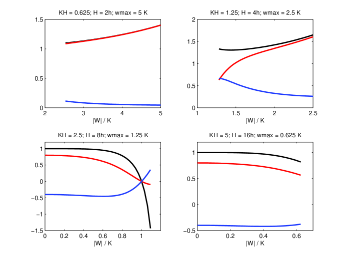
Figure 1: Symbol ratios for Fourier components visible on scale $H$; the $x$-axis variable is $|{\bf\omega}|/k$. The black (top) line shows the HML ratios (10); the red line (middle) and the blue line (bottom) are the real and the imaginary parts of the SL symbol ratios (11). The ratios shown are for components with $\omega_{1}=\omega_{2}$.

As Figure 1 suggests, operators $L^{H}$ and $M^{H}$ exhibit similar accuracy for high-frequency components but differ for the near-kernel (8) and for lower frequencies. More precisely, for

• $kH\leq 0.625$: all components with $\pi/2<\omega_{max}H\leq\pi$ are well approximated by $L^{H}$ and $M^{H}$: $\mathop{\rm Re}(\tau_{H}^{SL})\approx\tau_{H}^{HLM}$ are close to one, $\mathop{\rm Im}(\tau_{H}^{SL})\leq.1$;

• $kH=1.25$: all components with $\pi/2<\omega_{max}H\leq\pi$ are accurately approximated by $L^{H}$, they satisfy $(1+\alpha_{1})k\leq|{\bf\omega}|\leq 2(1+\alpha_{1})k$, $\alpha_{1}\approx.4$. The accuracy deteriorates for smoother components, in particular as $|w|$ approaches $k$. $M^{H}$ provides an accurate approximation for a smaller range of components, the ones with $(1+\beta_{1})\leq|{\bf\omega}|\leq 2(1+\alpha_{1})k$, $\beta_{1}\approx.8$. The growing imaginary part of $\tau_{H}^{SL}$ for smaller $|{\bf\omega}|$ affects the approximation quality. Both $L^{H}$ and $M^{H}$ fail to approximate components (8) though in a different way.

• $kH=2.5$: $L^{H}$ provides an accurate approximation for $|{\bf\omega}|\leq(1-\alpha_{0})k$, with $\alpha_{0}\approx.1$ and does not approximate components with $|{\bf\omega}|\geq k$; $M^{H}$ gives a rise to a wrong approximation for all components in question, though manages to do so in the right way (see the footnote);

• $kH=5$: all components visible on scale $H$, $0\leq|{\bf\omega}|\leq 0.65k$, have an accurate approximation by $L^{H}$, but not by $M^{H}$ (due to a large negative imaginary part).

To summarize, a sequence of coarse-grid Helmholtz operators $\{L^{H}\}_{H>h}$ accurately approximates the finest grid Helmholtz operator $L^{h}$ for all Fourier components except (8), more precisely with $(1-\alpha_{0})k\leq|{\bf\omega}|\leq(1+\alpha_{1})k$, with $\alpha_{0}\approx.1$ and $\alpha_{1}\approx.4$. Coarse-grid Shifted Laplacian operators $\{M^{H}\}_{H>h}$ approximate the finest-grid Helmholtz operator for all oscillatory components, failing to approximate both (8) and (unlike $L^{H}$) smooth error, more precisely, components with $0\leq|{\bf\omega}|\leq(1+\beta_{1})k$, with $\beta_{1}\approx.8$.

4 Gauss Seidel relaxation for $L^{H}$ and $M^{H}$

Application of one iteration of the lexicographic Gauss-Seidel relaxation to $L^{H}$ and $M^{H}$ yields the following amplitude change of an erroneous Fourier component $e^{i(\omega_{1}x+\omega_{2}y)}$

$$\mu_{H}^{HLM}(\theta_{1}^{H},\theta_{2}^{H})=\biggl{|}\frac{\exp(-i\theta_{1}^{H})+\exp(-i\theta_{2}^{H})}{\exp(i\theta_{1}^{H})+\exp(i\theta_{2}^{H})-4+k^{2}H^{2}}\biggr{|}$$ (12)

and

$$\mu_{H}^{SL}(\theta_{1}^{H},\theta_{2}^{H})=\biggl{|}\frac{\exp(-i\theta_{1}^{H})+\exp(-i\theta_{2}^{H})}{\exp(i\theta_{1}^{H})+\exp(i\theta_{2}^{H})-4+k^{2}(1+i\beta)H^{2}}\biggr{|}$$ (13)

for Helmholtz and Shifted Laplacian operators, respectively. Typically, in predicting a convergence rate of a multigrid solver, the smoothing properties of the relaxation is the main parameter. It is measured by a smoothing factor:

$$\tilde{\mu}_{H}=\max_{\pi/2\leq\max\{|\theta_{1}^{H}|,|\theta_{2}^{H}|\}\leq\pi}\mu_{H}(\theta_{1}^{H},\theta_{2}^{H}).$$ (14)

For $L^{H}$ and $M^{H}$ there is an additional phenomenon – divergence of smooth error component. To monitor that, an overall convergence rate is also considered:

$$\hat{\mu}_{H}=\max_{0\leq\max\{|\theta_{1}^{H}|,|\theta_{2}^{H}|\}\leq\pi}\mu_{H}(\theta_{1}^{H},\theta_{2}^{H});$$ (15)

$\hat{\mu}_{H}>1$ means divergence. Figure 2 shows $\mu_{H}(\omega_{1},\omega_{2})$ for $L^{H}$ and $M^{H}$ on increasingly coarse scales starting with the finest, $kh=0.3125$. It suggests that Gauss-Seidel relaxation performs similarly when applied to $L^{H}$ and $M^{H}$. In particular for

• $kH\leq 0.3125$: $\tilde{\mu}_{H}^{HLM}\approx\tilde{\mu}_{H}^{SL}\approx 0.5$ and $\hat{\mu}^{HLM}_{H}\approx\hat{\mu}_{H}^{SL}\leq 1.05$;

• $kH=0.625$: $\tilde{\mu}_{H}^{HLM}\approx\tilde{\mu}_{H}^{SL}\approx 0.7$ and $\hat{\mu}^{HLM}_{H}\approx\hat{\mu}_{H}^{SL}\leq 1.1$;

• $kH=1.25$: divergence of smooth error components becomes prohibitively large, with $\hat{\mu}^{HLM}_{H}\approx 4.5$ and $\hat{\mu}^{SL}_{H}\approx 3.5$; no error reduction for $|{\bf\omega}|\approx k$. However, error components with $|{\bf\omega}|\geq 1.3k$ for $L^{H}$ and with $|{\bf\omega}|\geq 1.8k$ for $M^{H}$ are reduced by at least the factor of $0.7$;

• $kH=2.5$: $\tilde{\mu}^{HLM}\approx\tilde{\mu}^{SL}\approx 1$ – no convergence for (8); for smooth components, $\mu^{HLM}_{H}(\omega_{1},\omega_{2})\leq 0.7$ for ($|{\bf\omega}|\leq.9k$) and $\mu^{SL}_{H}(\omega_{1},\omega_{2})\leq 0.7$ for ($|{\bf\omega}|\leq.8k$).

• $kH=5$: $\hat{\mu}^{HLM}_{H}\approx.1$ and $\hat{\mu}^{SL}_{H}\approx.085$ making a few relaxation sweeps an equivalent to a direct solver; no coarser grids are needed.
  

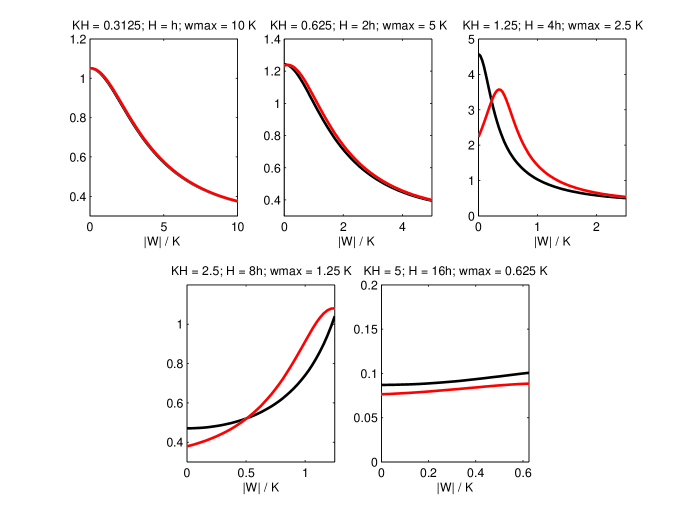
Figure 2: The black line shows the rates for Helmholtz operators; the red line - for Shifted Laplacian ones; convergence rates of Fourier components visible on scale $H$; the finest scale satisfies $kh=0.3125$; the $x$-axis variable is $|{\bf\omega}|/k$; results are shown for Fourier components with $\omega_{1}=\omega_{2}$;

Overall, Gauss-Seidel relaxation for both approaches performs well on scales with $kH\lessapprox 0.625$ and $kH\gtrapprox 2.5$. It fails to reduce near-kernel components (7) on any grid and diverges smooth error components when $kH\approx 1.25$. To avoid or diminish the latter effect, Gauss-Seidel is applied to the normal operator $(L^{H})^{T}L^{H}$ or $(M^{H})^{T}M^{H})$ instead of original $L^{H}$ or $M^{H}$, where ^T here means transposed, complex conjugate. This is done in the spirit of Kaczmarz iterations [8] known to be slow but convergent. The number of relaxation sweeps on this scale is higher than on others.

Remark 4.1.

The actual constants in the discussion above as well as in Section 3 are partial for the chosen parameters; they aim at giving a qualitative understanding of the processes described. While the study is conducted for Gauss-Seidel iterations, similar conclusions, with slightly different constants, can be made for other linear iterative schemes such as Jacobi or SOR.

5 Optimal algorithm

A multigrid V-cycle is applied to (1) in three variants. It employs:

• Operators $L^{H}$ and/or $M^{H}$, second-order FD discretizations of $L$ and $M$ with five-point stencils;

• bilinear interpolation;

• full weighting;

• Gauss-Seidel iterations:

  • one pre- and post-smoothing steps on all scales except $kH\approx 1.25$, applied either to $L^{H}$ or to $M^{H}$;

  • four pre- and post-smoothing steps on scale $kH\approx 1.25$, applied either to $(L^{H})^{T}L^{H}$ or to $(M^{H})^{T}M^{H}$.

On each scale a coarse-grid operator is used in two capacities:

1. for relaxation;

2. for computing coarse-grid residuals.

Three variants are considered:

• HLM-V employs $L^{H}$ both for (A) and for (B);

• SL-V employs $M^{H}$ both for (A) and for (B)

• HYB-V always employs $L^{H}$ for (B). $L^{H}$ is also used for (A) on all grids except $0.625\lessapprox kH\lessapprox 1.25$ where it is replaced by $M^{H}$.

The motivation for the hybrid method comes from observations reported in Sections 3 and 4 concerning performance of SL and HLM operators on intermediate and coarse scales. (On finer grids both act very similarly, and either one can be used.) The strength of the Shifted Laplacian approach, studied in detail in [5, 6], is the transformation (not reduction) of the near-kernel error components, that mostly occurs on intermediate scales. This is the reason for employing $M^{H}$ in relaxation there.

On coarse grids, however, Helmholtz operators $L^{H}$, give a rise to an accurate approximation of smooth components, and, together with a fast convergence by Gauss-Seidel there, allow for an efficient coarse-grid correction. Therefore, $L^{H}$ is used in relaxation on the coarsest scale(s).

6 Numerical Experiments and Computational Costs

The V-cycle based variants, along with the original Shifted Laplacian (OSL) [6] multigrid preconditioner, are compared, and their computational costs are discussed. Bi-CGSTAB serves as an outer iteration. Also briefly introduced is the idea of the ray correction [1], and numerical results for HLM, SL and HYB, enriched by it, are presented.

6.1 Numerical results

First, the algorithms are tested for (1) with a constant $k$, considered on $\Omega=[0,1]^{2}$, and the results are presented in Table 1. Initial approximations $x^{0}$ are zero in all experiments; iterations are performed until the initial residual $\|r^{0}\|=\|f\|$ is reduced by a factor of $10^{7}$. In Tables 1-2, right-hand-sides are homogeneous except at the center of $\Omega$, where $f(.5,.5)=1$;

$k$	40	50	80	100	150
$h$	$1/64$	$1/80$	$1/128$	$1/160$	$1/240$
OSL	26	31	44	52	73
SL-V	19	24	27.5	31	38
HYB-V	16	20.5	23	26.5	31.5

Table 1: The number of Bi-CGSTAB iterations for different preconditioners and values of constant wave numbers; in all experiments $kh=0.625$.

The results show that both the SL-V and HYB-V preconditioners are more efficient than OSL, and the hybrid approach outperforms the Shifted Laplacian.

In Table 2, performance of SL-V and HYB-V methods is tested for the same model problem when considered on increasingly finer $h$; both show an improved convergence while computing increasingly accurate solutions.

$h$	1/64	1/128	1/256	1/512
SL-V	19	18	17.5	16
HYB-V	16	15.5	15	14

Table 2: The number of Bi-CGSTAB iterations; $k=40$, $kh$ ranges from $0.625$ to $0.078125$.

Next considered is (1) with a heterogeneous medium - a wedge problem shown in Figure 3, with numerical experiments presented in Table 3. Again, the hybrid preconditioner performs better than the Shifted Laplacian does.

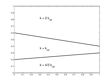
Figure 3: Wave number distribution in the wedge problem The point source is located at the middle of the upper boundary: $f(0.5,1.)=1$ and zero elsewhere. The choice of $k(x)$ is in spirit of the wedge example in [6]. The domain remains $[0,1]^{2}$.

$k_{ref}$	15	30	60	120	240
SL-V	13	18.5	33	49.5	61
HYB-V	9.5	14	23	36.5	41

Table 3: The number of Bi-CGSTAB iterations for SL-V and HYB-V preconditioners; in all experiments $k_{ref}h\approx 0.2344$; the value of $k$ in the Table varies from $15$ to $480$.

Our experiments are performed for a slightly different problem that the ones reported in [6]. We mention, however, that in [6] the experiments were performed for $k\leq k_{max}=240$, which arises for $k_{ref}=120$, and it required $66$ Bi-CGSTAB iterations. Our experiments with the same $k_{ref}=120$ (and $k_{max}=240$) require only $36.5$ Bi-CGSTAB iterations with HYB preconditioner.

Noticeably missing from action so far is HLM-V approach, and this is because its acceleration of Bi-CGSTAB or other Krylov methods, is inferior to the SL-based algorithms. This changes, however, when the ray multigrid approach [1] is used as an additional coarse-grid correction, [10, 1, 11]. It is based on the assumption that the near-kernel error components (8) can be represented as

$$e=\sum_{j=1}^{8}\hat{a}_{j}e^{i(k_{1}^{j}x+k_{2}^{j}y)},\quad(k_{j}^{1},k_{j}^{2})=k\biggl{(}\cos\,\frac{j\pi}{4},\sin\,\frac{j\pi}{4}\biggr{)},$$ (16)

with smooth ray functions $\hat{a}_{j}$. The idea is than to reduce the task of computing $e$ to a much easier task of approximating each $\hat{a}_{j}$ individually on some coarse scale. This process itself reduces a range of the near-kernel Fourier error components with $(1-\gamma_{0})k\leq|{\bf\omega}|\leq(1+\gamma_{1})k$. Constants $\gamma_{0},\gamma_{1}$ depend on relaxation strategy and problem parameters: typical values are $\gamma_{0}\approx\gamma_{1}\approx 0.3$. This means that all error components not well approximated/well reduced by HLM-V are in this range, and they are all treated by the ray correction. Results for HLM-V, HYB-V and SL-V cycles, accelerated by the ray correction, are presented in Table 4. No Krylov outer iterations are employed: each method serves as a solver rather than a preconditioner; HLM-V cycle with the ray correction is the original wave-ray algorithm. The cost of each iteration in this Table is about twice lower than iteration costs in other Tables, where one Bi-CGSTAB employs a multigrid preconditioner twice.

$k$	20	40	80	160
HLM-V	16	16	17	18
SL-V	23	34	41	48
HYB-V	26	31	37	39

Table 4: The number of V-cycles using HLM-V, SL-V and HYB-V approaches enhanced by the ray correction; in all experiments $kh=0.3125$; $f(.5,.5)=0$, and it is zero elsewhere.

6.2 Computational Costs

Costs of SL-V, HLM-V, and HYB-V preconditioners are close to costs of a standard multigrid $V(1,1)$ cycle applied to a Laplace operator; the main difference is the cost of the extra six relaxation sweeps applied to the normal equation on scale with $kH\approx 1.25$ (Six is eight per level minus standard two per grid in $V(1,1))$. While the absolute cost of these iterations remains the same for a given (1), its relative fraction in the overall costs becomes smaller when (3) is discretized on finer scale $h$. The OSL preconditioner is implemented differently from the algorithms discussed here: it employs a $F(1,1)$ cycle in the algebraic multigrid framework using the operator dependent-interpolation based on de Zeewv’s transfer operators [2]. The $F(1,1)$ cycle becomes more expensive (in computational costs) than our almost $V(1,1)$ cycle starting with $kh=0.3125$ and finer.

7 Conclusions

Standard multigrid V-cycle is applied to the Helmholtz and the Shifted Laplacian operators, and the resulting algorithms are employed as preconditioners for Bi-CGSTAB, used to solve the indefinite Helmholtz equations. The Shifted Laplacian approach shows a superior performance. However, after analyzing approximation and relaxation properties of both operators, a hybrid method, a combination of the two, is proposed, yielding an improved convergence. With the ray correction, the HLM approach works significantly better - resulting in a well scalable algorithm with convergence nearly independent on wave numbers.

References

- [1] A. Brandt and I. Livshits. Wave-ray multigrid method for standing wave equations. Electron. Trans. Numer. Anal., pages 162–181, 1997.
- [2] P.M. de Zeewv. Matrix dependent prolongations and restrictions in a blackbox multigrid solver. J. Computational and Applied Mathematics, 33:1–27, 1990.
- [3] H. C. Elman, O. G. Ernst, and D. P. O’Leary. A multigrid method enhanced by krylov subspace iteration for discrete helmholtz equations. SIAM J. Sci. Comput., 23(4):1291–1315, 2001.
- [4] B. Engquist and L. Ying. Sweeping preconditioner for the helmholtz equation: hierarchical matrix representation. Comm. Pure Appl. Math., 64:697––735, 2011.
- [5] Y. A. Erlangga, C. W. Oosterlee, and C. Vuik. A novel multigrid based preconditioner for heterogeneous helmholtz problems. SIAM J. Sci. Comput., 27(4):1471–1492, 2006.
- [6] Y. A. Erlangga, C. Vuik, and C. W. Oosterlee. On a class of preconditioners for solving the helmholtz equation. Appl. Numer. Math., 50(3-4):40–425, 2004.
- [7] E. Haber and S. MacLachlan. A fast method for the solution of the helmholtz equation. J. Comp. Phys., 230:4403––4418, 2011.
- [8] S. Kaczmarz. Angenaherte auflosung von systemen linearer gleichungen. Bulletin International de l’Académia Polonaise des Sciences et des Lettres. Classe des Sciences Mathématiques et Naturalles. Série A., Sciences Mathématiques, 35:355–357, 1937.
- [9] B. Lee, T. A. Manteuffel, S. F. McCormick, and J. Ruge. First-order system leastsquares for the helmholtz equation. SIAM J. Sci. Comput., 21(5):1927–1949, 2000.
- [10] I. Livshits. Ph. D. Thesis. Bar Ilan University, Israel, 1997.
- [11] I. Livshits and A. Brandt. Accuracy properties of the wave-ray multigrid algorithm for helmholtz equations. SIAM J. Sci. Comput., 28(4):1228 –1251, 2006.
- [12] P.-G. Martinsson and V. Rokhlin. A fast direct solver for scattering problems involving elongated structures. J. Comput. Phys., 221(1):288–302, 2007.
- [13] P. Vanek, J.Mandel, and M.Brezina. Two-level algebraic multigrid for the helmholtz problem. In Domain decomposition methods 10, 218:349–356, 1998.