Abstract.

Quasi steady state assumptions are often used to simplify complex systems of ordinary differential equations in modelling of biochemical processes. The simplified system is designed to have the same qualitative properties as the original system and to have a small number of variables. This enables to use the stability and bifurcation analysis to reveal a deeper structure in the dynamics of the original system. This contribution shows that introducing delays to quasi steady state assumptions yields a simplified system that accurately agrees with the original system not only qualitatively but also quantitatively. We derive the proper size of the delays for a particular model of circadian rhythms and present numerical results showing the accuracy of this approach.

Keywords: biochemical networks, gene regulatory networks, oscillating systems, periodic solutions, model reduction, accurate approximation

MSC 2010: 92C45, 92B25, 80A30, 34C15, 34C23

1. Introduction

Model reduction is a crucial technique in large biochemical systems, because it enables to employ analytical and numerical methods to reveal detailed structure of the kinetics [2, 3]. As an example, we consider a theoretical biochemical model of circadian rhythms described in [9]. Using the law of mass action [6], the kinetics of this chemical system can be described by a system of nine nonlinear ordinary differential equations (ODEs). The authors of [9] use various quasi steady state assumptions to reduce the system to just two ODEs in such a way that the reduced system has the same qualitative behaviour as the original system, i.e. a periodic solution. Then, they use the reduced system to perform the bifurcation and stochastic analysis.

However, using parameters introduced in [9], the period of the original system is about 25 hours while the period of the reduced system is roughly 18 hours. Thus, the relative error in the period is approximately 30 %. The error in the amplitude is even close to 100 %, as we show in Table 1 below.

In this contribution we study the quasi steady state assumptions in detail. We use numerical quadrature to derive explicit formulas for delays for approximated chemical species and reduce the original system of nine chemical reactions to two delay ODEs. Some of the delays depend on the state variables in a complicated way, which might be problematic for the subsequent analysis, therefore we show that this dependence can be simplified. Finally, numerical solutions show that periods of the original and reduced system agree within 2 % relative error and that the error in the amplitude decreases to about 20 %.

The following section introduces the model of circadian rhythms and its quasi steady state reduction. Section 3 justifies the quasi steady state assumptions and Section 4 derives the delayed quasi steady state assumption. The accuracy of these approximations is assessed in Section 6 and final conclusions are drawn in Section 7.

2. Model of circadian rhythms

Circadian rhythms are modelled in [9] by the following system of nine ODEs:

(2.1) $$\mathrm{d}D_{A}/\mathrm{d}t =\theta_{A}D_{A}^{\prime}-\gamma_{A}D_{A}A,$$

(2.2) $$\mathrm{d}D_{A}^{\prime}/\mathrm{d}t =-\theta_{A}D_{A}^{\prime}+\gamma_{A}D_{A}A,$$

(2.3) $$\mathrm{d}D_{R}/\mathrm{d}t =\theta_{R}D_{R}^{\prime}-\gamma_{R}D_{R}A,$$

(2.4) $$\mathrm{d}D_{R}^{\prime}/\mathrm{d}t =-\theta_{R}D_{R}^{\prime}+\gamma_{R}D_{R}A,$$

(2.5) $$\mathrm{d}M_{A}/\mathrm{d}t =\alpha_{A}^{\prime}D_{A}^{\prime}+\alpha_{A}D_{A}-\delta_{M_{A}}M_{A},$$

(2.6) $$\mathrm{d}M_{R}/\mathrm{d}t =\alpha_{R}^{\prime}D_{R}^{\prime}+\alpha_{R}D_{R}-\delta_{M_{R}}M_{R},$$

(2.7) $$\mathrm{d}A/\mathrm{d}t =\beta_{A}M_{A}+\theta_{A}D_{A}^{\prime}+\theta_{R}{D_{R}^{\prime}}-A(\gamma_{A}D_{A}+\gamma_{R}D_{R}+\gamma_{C}R+\delta_{A}),$$

(2.8) $$\mathrm{d}R/\mathrm{d}t =\beta_{R}M_{R}-\gamma_{C}AR+\delta_{A}C-\delta_{R}R,$$

(2.9) $$\mathrm{d}C/\mathrm{d}t =\gamma_{C}AR-\delta_{A}C.$$

Here, the time variable is denoted by $t$, the capital letters stand for the copy numbers of respective molecules that evolve in time and Greek letters stand for the rate constants. Namely, $A=A(t)$, $R=R(t)$, $M_{A}=M_{A}(t)$, $M_{R}=M_{R}(t)$, $D_{A}=D_{A}(t)$, $D_{R}=D_{R}(t)$ denote the numbers of molecules of the activator, represor, their mRNA and genes, respectively. Functions $D_{A}^{\prime}=D_{A}^{\prime}(t)$ and $D_{R}^{\prime}=D_{R}^{\prime}(t)$ stand for the number of molecules of the activated forms of genes and $C=C(t)$ for the complex of $A$ and $R$. Values for the rate constants are taken from [9] as

(2.10) $$\alpha_{A}=50\,\mathrm{h}^{-1},\ \alpha_{A}^{\prime}=500\,\mathrm{h}^{-1},\ \alpha_{R}=0.01\,\mathrm{h}^{-1},\ \alpha_{R}^{\prime}=50\,\mathrm{h}^{-1},\ \beta_{A}=50\,\mathrm{h}^{-1},\\ \beta_{R}=5\,\mathrm{h}^{-1},\ \gamma_{A}=1\,\mathrm{Mol}^{-1}\mathrm{h}^{-1},\ \gamma_{R}=1\,\mathrm{Mol}^{-1}\mathrm{h}^{-1},\ \gamma_{C}=2\,\mathrm{Mol}^{-1}\mathrm{h}^{-1},\ \delta_{A}=1\,\mathrm{h}^{-1},\\ \delta_{R}=0.2\,\mathrm{h}^{-1},\ \delta_{M_{A}}=10\,\mathrm{h}^{-1},\ \delta_{M_{R}}=0.5\,\mathrm{h}^{-1},\ \theta_{A}=50\,\mathrm{h}^{-1},\ \theta_{R}=100\,\mathrm{h}^{-1}.$$

Notice that by Mol and h we understand the number of molecules and the hour. The initial condition for system (2.1)–(2.9) is considered as

(2.11) $$D_{A}=D_{R}=1\,\mathrm{Mol},\quad D_{A}^{\prime}=D_{R}^{\prime}=M_{A}=M_{R}=A=R=C=0\,\mathrm{Mol}.$$

Figure 1 shows three components of the solution of system (2.1)–(2.9) with parameter values (2.10) and initial condition (2.11) as solid lines.

To reduce the system, let us first notice that $\mathrm{d}(D_{A}+D_{A}^{\prime})/\mathrm{d}t=0$ and $\mathrm{d}(D_{R}+D_{R}^{\prime})/\mathrm{d}t=0$. Thus, due to the initial condition we infer conservation relations

(2.12) $$D_{A}^{\prime}=1-D_{A}\quad\text{and}\quad D_{R}^{\prime}=1-D_{R}$$

that enable to eliminate $D_{A}^{\prime}$ and $D_{R}^{\prime}$ from the system by simple substitution. To simplify the system further we use so-called quasi steady state assumptions [5, 7].

In general, the idea of quasi steady state assumptions is based on splitting the system into slow and fast variables. The steady state of fast variables depends on values of slow variables. If slow variables change, the steady states change as well and the fast variables go quickly towards their new steady states. Thus it is a reasonable approximation to consider the fast variables to be effectively in their steady states. Of course, the quality of this approximation depends on actual speeds of the dynamics of the slow and fast variables.

In case of system (2.1)–(2.9), we simply assume that $D_{A}$, $D_{R}$, $M_{A}$, $M_{R}$, and $A$ are fast and stay in their steady states that may however change with the values of the slow variables $R$ and $C$. From (2.1), (2.3), (2.5), and (2.6) with (2.12), we easily obtain steady states for $D_{A}$, $D_{R}$, $M_{A}$ and $M_{R}$ as functions of $A$:

(2.13) $$D_{A}^{s}(A) =\frac{\theta_{A}}{\theta_{A}+\gamma_{A}A}, \qquad M_{A}^{s}(A) =\frac{\alpha_{A}^{\prime}}{\delta_{M_{A}}}+\frac{\theta_{A}(\alpha_{A}-\alpha_{A}^{\prime})}{\delta_{M_{A}}(\theta_{A}+\gamma_{A}A)},$$

$$D_{R}^{s}(A) =\frac{\theta_{R}}{\theta_{R}+\gamma_{R}A}, \qquad M_{R}^{s}(A) =\frac{\alpha_{R}^{\prime}}{\delta_{M_{R}}}+\frac{\theta_{R}(\alpha_{R}-\alpha_{R}^{\prime})}{\delta_{M_{R}}(\theta_{R}+\gamma_{R}A)}.$$

Approximating $D_{A}$, $D_{R}$, $M_{A}$, and $M_{R}$ by their respective steady states in (2.7), we can express the steady state of $A$ as the following function of $R$:

(2.14) $$\widetilde{A}^{s}(R)=\frac{1}{2}(\alpha_{A}^{\prime}\rho(R)-K_{d})+\frac{1}{2}\sqrt{(\alpha_{A}^{\prime}\rho(R)-K_{d})^{2}+4\alpha_{A}\rho(R)K_{d}},$$

where $\rho(R)=\beta_{A}/(\delta_{M_{A}}(\gamma_{C}R+\delta_{A}))$ and $K_{d}=\theta_{A}/\gamma_{A}$, see [9]. Using the approximation $A=\widetilde{A}^{s}(R)$, we may express steady states (2.13) as functions of $R$ and reduce the original system (2.1)–(2.9) to just two ODEs for $R$ and $C$:

(2.15) $$\mathrm{d}R/\mathrm{d}t =\beta_{R}M_{R}^{s}(\widetilde{A}^{s}(R))-\gamma_{C}\widetilde{A}^{s}(R)R+\delta_{A}C-\delta_{R}R,$$

(2.16) $$\mathrm{d}C/\mathrm{d}t =\gamma_{C}\widetilde{A}^{s}(R)R-\delta_{A}C.$$

Figure 1 (left panel) shows $R(t)$ as the solution of (2.15)–(2.16) together with approximations of $D_{R}=D_{R}^{s}(\widetilde{A}^{s}(R))$ and $M_{R}=M_{R}^{s}(\widetilde{A}^{s}(R))$ as dashed lines.

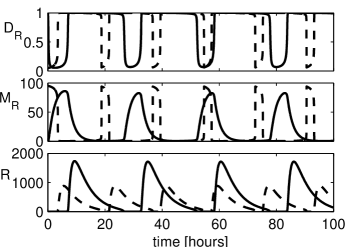
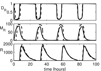
Figure 1. Components $D_{R}$, $M_{R}$, and $R$ of the solution of the original system (2.1)–(2.9) (solid lines), reduced system (2.15)–(2.16) (dashed lines, left panel), and delay system (5.7)–(5.8) (dashed lines, right panel).

3. Justification of quasi steady state assumptions

Let us justify the above described quasi steady state assumptions on an illustrative example of equation (2.5). Using (2.12), we can express equation (2.5) as

(3.1) $$\mathrm{d}M_{A}(t)/\mathrm{d}t=\Phi(t)-\delta_{M_{A}}M_{A}(t),\quad\text{where }\Phi(t)=\alpha_{A}^{\prime}+(\alpha_{A}-\alpha_{A}^{\prime})D_{A}(t).$$

If the function $\Phi(t)$ was explicitly known, we could easily find an expression for the solution $M_{A}(t)$ to (3.1) with the initial condition (2.11) as

(3.2) $$M_{A}(t)=\int_{0}^{t}\Phi(\tau)\exp[\delta_{M_{A}}(\tau-t)]\,\mathrm{d}\tau.$$

To obtain a quasi steady state approximation of $M_{A}(t)$ we employ one-point numerical quadrature in (3.2) and approximate $M_{A}(t)\approx w_{1}\Phi(t_{1})$, where $t_{1}=t$ is the quadrature point and the corresponding quadrature weight $w_{1}$ is determined such that the resulting rule integrates constant functions exactly: $w_{1}=\int_{0}^{t}\exp[\delta_{M_{A}}(\tau-t)]\,\mathrm{d}\tau=(1-\exp(-\delta_{M_{A}}t))/\delta_{M_{A}}$. Since the exponential function $\exp(-\delta_{M_{A}}t)$ decays quickly to zero, we may neglect it with respect to 1 for sufficiently large $t$. As a result we approximate $w_{1}\approx 1/\delta_{M_{A}}$ and $M_{A}(t)\approx\Phi(t)/\delta_{M_{A}}$ which is exactly the quasi steady state approximation $M_{A}^{s}(A)$ from (2.13) provided $D_{A}=D_{A}^{s}(A)$.

4. Derivation of delayed quasi steady state assumptions

The reasoning from the previous section can be made more accurate, because one-point quadrature rules have the capability to be exact even for all linear functions. More precisely, we consider a quadrature point $t_{2}=t-\tau_{M_{A}}$, a corresponding weight $w_{2}$, and approximate the integral in (3.2) by $w_{2}\Phi(t_{2})$. We find the particular values of $\tau_{M_{A}}$ and $w_{2}$ such that this quadrature rule is exact for all linear functions.

Any linear function can be expressed as $\ell(\tau)=\alpha_{1}\ell_{1}(\tau)+\alpha_{2}\ell_{2}(\tau)$, where $\ell_{1}(\tau)=(\tau+\tau_{M_{A}}-t)/\tau_{M_{A}}$ and $\ell_{2}(\tau)=(t-\tau)/\tau_{M_{A}}$. Clearly, $\ell$ is determined by its values $\alpha_{1}$ and $\alpha_{2}$ at points $t_{1}=t$ and $t_{2}=t-\tau_{M_{A}}$. Thus, the requirement of exactness for all linear functions can be formulated as

$$w_{2}\alpha_{2}=\int_{0}^{t}\ell(\tau)\exp[\delta_{M_{A}}(\tau-t)]\,\mathrm{d}\tau=\frac{1-(1+\delta_{M_{A}}t)\exp(-\delta_{M_{A}}t)}{\tau_{M_{A}}\delta_{M_{A}}^{2}}\alpha_{2}\\ +\frac{(1+\delta_{M_{A}}(t-\tau_{M_{A}}))\exp(-\delta_{M_{A}}t)-1+\delta_{M_{A}}\tau_{M_{A}}}{\tau_{M_{A}}\delta_{M_{A}}^{2}}\alpha_{1}.$$

This equality is satisfied for all $\alpha_{1}$ and $\alpha_{2}$ if

$$\tau_{M_{A}}=\frac{1-(1+\delta_{M_{A}}t)\exp(-\delta_{M_{A}}t)}{\delta_{M_{A}}(1-\exp(-\delta_{M_{A}}t))}\quad\text{and}\quad w_{2}=\frac{1-\exp(-\delta_{M_{A}}t)}{\delta_{M_{A}}}.$$

As above, since the exponential $\exp(-\delta_{M_{A}}t)$ decays rapidly towards zero, we can simplify the expressions for $\tau_{M_{A}}$ and $w_{2}$ to $\tau_{M_{A}}=1/\delta_{M_{A}}$ and $w_{2}=1/\delta_{M_{A}}$.

Consequently, the variable $M_{A}$ can be approximated as $M_{A}(t)=w_{2}\Phi(t-\tau_{M_{A}})=(\alpha_{A}^{\prime}+(\alpha_{A}-\alpha_{A}^{\prime})D_{A}(t-\tau_{M_{A}}))/\delta_{M_{A}}$. Clearly, this is the steady state value of $M_{A}$ evaluated at time delayed by $\tau_{M_{A}}=1/\delta_{M_{A}}$.

5. Delayed quasi steady state approximation of the circadian system

Delayed quasi steady state assumptions derived above are now applied to equations (2.1)–(2.7). All these equations have the same structure, namely

(5.1) $$\mathrm{d}X(t)/\mathrm{d}t=f(t)-g(t)X(t)$$

for suitably chosen coefficients $f(t)$ and $g(t)$. The template derivation performed above for equation (2.5) is now used for equation (5.1) and we define formally its time delay as $\tau_{X}(t)=1/g(t)$ and its delayed quasi steady state approximation as $X^{\tau}(t)=f(t-\tau_{X}(t))/g(t-\tau_{X}(t))$.

Applying this methodology to (2.1)–(2.7) with (2.12), we obtain the following delays and approximations:

(5.2) $$\tau_{D_{A}}(t) =\left[\theta_{A}+\gamma_{A}\widetilde{A}^{s}(R(t))\right]^{-1}, \quad D_{A}^{\tau}(t) =D_{A}^{s}(A^{\tau}(t-\tau_{D_{A}}(t))),$$

(5.3) $$\tau_{D_{R}}(t) =\left[\theta_{R}+\gamma_{R}\widetilde{A}^{s}(R(t))\right]^{-1}, \quad D_{R}^{\tau}(t) =D_{R}^{s}(A^{\tau}(t-\tau_{D_{R}}(t))),$$

(5.4) $$\tau_{M_{A}} =\delta_{M_{A}}^{-1}, \quad M_{A}^{\tau}(t) =M_{A}^{s}(A^{\tau}(t-\tau_{M_{A}})),$$

(5.5) $$\tau_{M_{R}} =\delta_{M_{R}}^{-1}, \quad M_{R}^{\tau}(t) =M_{R}^{s}(A^{\tau}(t-\tau_{M_{R}})),$$

(5.6) $$\tau_{A}(t) =\makebox[113.81102pt][l]{$[\gamma_{A}D_{A}^{\tau}(t)+\gamma_{R}D_{R}^{\tau}(t)+\gamma_{C}R(t)+\delta_{A}]^{-1},$} \qquad\quad A^{\tau}(t)=A^{s}(t-\tau_{A}(t)),$$

where the definition of $A^{s}$ comes directly from (2.7) with (2.12) and reads as

$$A^{s}(t)=\frac{\beta_{A}M_{A}^{\tau}(t)+\theta_{A}(1-D_{A}^{\tau}(t))+\theta_{R}(1-D_{R}^{\tau}(t))}{\gamma_{A}D_{A}^{\tau}(t)+\gamma_{R}D_{R}^{\tau}(t)+\gamma_{C}R+\delta_{A}}.$$

Note that $\widetilde{A}^{s}$ was defined already in (2.14).

The remaining two variables $R$ and $C$ are naturally computed by their ODEs (2.8)–(2.9), where $M_{R}$ and $A$ are replaced by their respective approximations:

(5.7) $$\mathrm{d}R(t)/\mathrm{d}t =\beta_{R}M_{R}^{\tau}(t)-\gamma_{C}A^{\tau}(t)R(t)+\delta_{A}C(t)-\delta_{R}R(t),$$

(5.8) $$\mathrm{d}C(t)/\mathrm{d}t =\gamma_{C}A^{\tau}(t)R(t)-\delta_{A}C(t).$$

To solve this system of delayed differential equations, we constantly extend the initial conditions (2.11) to the interval $(-\infty,0]$.

System (5.7)–(5.8) with (5.2)–(5.6) is a system of delay differential equations with state dependent delays [4]. The dependence of the delays on $R$ is complicated, but it can be simplified. Instead of variable delays $\tau_{D_{A}}(t)$, $\tau_{D_{R}}(t)$, and $\tau_{A}(t)$ we may consider constant delays $\tau_{D_{A}}^{*}=1/\theta_{A}$, $\tau_{D_{R}}^{*}=1/\theta_{R}$, and state dependent delay $\tau_{A}^{*}(t)=1/(\gamma_{C}R(t)+\delta_{A})$. The effect of this simplification is numerically assessed in the following section.

6. Numerical assessment of the accuracy

System (5.7)–(5.8) with (5.2)–(5.6) can be easily solved numerically. We obtained high accuracy by implicit Euler method with time step $10^{-3}$ h. Three components of this numerical solution are presented in Figure 1 (right panel) as dashed lines.

Comparing the two panels in Figure 1 we clearly see that delayed approximations are much more accurate. However, in order to quantify the accuracy we measure and compare both the period and amplitude of oscillations.

Let $\boldsymbol{f}(t)=(D_{A},D_{A}^{\prime},D_{R},D_{R}^{\prime},M_{A},M_{R},A,R,C)(t)$ be the solution of the original system (2.1)–(2.9). Except for an initial transient, it is a periodic vector with period $p_{\mathrm{orig}}$. Similarly, let $\boldsymbol{g}(t)$ be a solution of one of the approximate systems described above and let its period be $p_{\mathrm{approx}}$. To quantify the accuracy of proposed approximations, we define the relative error in the period and the relative $L^{2}$-error as

$$\mathrm{RelErr}(\mathrm{period})=\frac{|p_{\mathrm{orig}}-p_{\mathrm{approx}}|}{p_{\mathrm{orig}}}\quad\text{and}\quad\mathrm{RelErr}(L^{2})=\frac{\|\boldsymbol{f}-\widetilde{\boldsymbol{g}}\|_{L^{2}(a,b)}}{\|\boldsymbol{f}\|_{L^{2}(a,b)}},$$

where $b-a=p_{\mathrm{orig}}$ and $\widetilde{\boldsymbol{g}}$ is linearly scaled and shifted vector $\boldsymbol{g}$ such that the error in period is eliminated. In particular, $\widetilde{\boldsymbol{g}}$ is linearly scaled such that its period is exactly $p_{\mathrm{orig}}$ and it is shifted such that local maxima of $\boldsymbol{f}$ and $\widetilde{\boldsymbol{g}}$ match.

Table 1 presents periods and relative errors for the original system (2.1)–(2.9) and for its various approximations. Namely, the third column corresponds to problem (2.15)–(2.16), which is the original system simplified by standard quasi steady state assumptions. The fourth column shows problem (5.7)–(5.8) with delays (5.2)–(5.6) and the fifth column presents the same problem with simplified delays $\tau_{D_{A}}^{*}$, $\tau_{D_{R}}^{*}$, and $\tau_{A}^{*}$. The last column corresponds to the same case as the fifth, but the only state dependent delay $\tau_{A}^{*}$ is replaced by constant delay $\tau_{A}^{**}=\tau_{M_{A}}$.

	original	approximations
	system	standard	derived	simplified	constant
		(no delays)	delays	delays	delays
period	25.6 h	17.9 h	25.1 h	25.3 h	26.1 h
$\mathrm{RelErr}(\mathrm{period})$	—	29.8 %	1.65 %	1.02 %	2.28 %
$\mathrm{RelErr}(L^{2})$	—	92.7 %	19.0 %	19.0 %	22.7 %

Table 1. Period and relative errors for various approximations.

We clearly observe quantitatively poor approximation properties of the standard quasi steady state assumptions. However, introducing delays yields approximations with relative errors in the period about 1–2 % only. The amplitude and the actual shape of the solution measured by relative $L^{2}$-error considerably improved as well.

7. Conclusions

Results presented above indicate that introducing delays to standard quasi steady state assumptions considerably improves the quantitative accuracy of the reduced system. Further, the derivation based on quadrature formulas results in explicit expressions for the actual size of the delays. The presented numerical results demonstrate the accuracy of the proposed approach and show that the derived complicated dependence of delays on the state variables can be simplified up to constant delays.

Since the studied model of circadian rhythms is based on standard biochemical processes such as transcription and translation, the presented technique of delayed quasi steady state assumptions can be easily applied to many other biochemical networks. The simplest case is the kinetics of mRNA, where the derived delays are constant and inversely proportional to the decay rates $\delta_{A}$ and $\delta_{R}$. More complicated expressions for delays were derived in the case of genes. However, their fast kinetics and the fact that there is just one molecule of DNA in a cell enables to simplify these delays to constants with practically no influence on the accuracy. Finally, the complicated dependence of delays on the state variables for some proteins can be simplified up to constant delays.

Certain mathematical models of gene expression are based on ODEs [9, 10] others are based on delay differential equations [1, 8]. The presented study may contribute to the understanding of the connection between these models and it may suggest that models with and without delays are just two sides of the same coin.

Authors’ addresses: Tomáš Vejchodský, University of Oxford, Mathematical Institute, Radcliffe Observatory Quarter, Woodstock Road, Oxford, OX2 6GG, United Kingdom; and Institute of Mathematics, Academy of Sciences, Žitná 25, Praha 1, CZ-115 67, Czech Republic; e-mail: vejchod@math.cas.cz.

References

• [1] L. Chen, K. Aihara: Stability of genetic regulatory networks with time delay. IEEE Trans. Circuits Systems I Fund. Theory Appl. 49 (2002), 602–608. MR1909315
• [2] S. Cotter, T. Vejchodský, R. Erban: Adaptive finite element method assisted by stochastic simulation of chemical systems. SIAM J. Sci. Comput. 35 (2013), B107–B131. Zbl 1264.65158, MR3033062
• [3] R. Erban, S.J. Chapman, I.G. Kevrekidis, T. Vejchodský: Analysis of a stochastic chemical system close to a sniper bifurcation of its mean-field model. SIAM J. Appl. Math. 70 (2009), 984–1016. Zbl 1200.80010, MR2538635
• [4] Y. Kuang: Delay differential equations with applications in population dynamics. Academic Press, Boston, MA, 1993. Zbl 0777.34002, MR1218880
• [5] J.D. Murray: Mathematical biology. I. An introduction. Springer-Verlag, New York, 2002. Zbl 1006.92001, MR1908418
• [6] M. Savageau: Biochemical systems analysis: I. some mathematical properties of the rate law for the component enzymatic reactions. J. Theoret. Biol. 25 (1969), 365–369.
• [7] L.A. Segel, M. Slemrod: The quasi-steady-state assumption: a case study in perturbation. SIAM Rev. 31 (1989), 446–477. Zbl 0679.34066, MR1012300.
• [8] A. Verdugo, R. Rand: Hopf bifurcation in a DDE model of gene expression. Commun. Nonlinear Sci. Numer. Simul. 13 (2008), 235–242. Zbl 1134.34325, MR2360687
• [9] J.M.G. Vilar, H.Y. Kueh, N. Barkai, S. Leibler: Mechanisms of noise-resistance in genetic oscillators. PNAS 99 (2002), 5988–5992.
• [10] Z. Xie, D. Kulasiri: Modelling of circadian rhythms in Drosophila incorporating the interlocked PER/TIM and VRI/PDP1 feedback loops. J. Theoret. Biol. 245 (2007), 290–304. MR2306447