Abstract

Many combinatorial problems can be formulated as “Can I transform configuration 1 into configuration 2, if certain transformations only are allowed?”. An example of such a question is: given two $k$-colourings of a graph, can I transform the first $k$-colouring into the second one, by recolouring one vertex at a time, and always maintaining a proper $k$-colouring? Another example is: given two solutions of a SAT-instance, can I transform the first solution into the second one, by changing the truth value one variable at a time, and always maintaining a solution of the SAT-instance? Other examples can be found in many classical puzzles, such as the 15-Puzzle and Rubik’s Cube.

In this survey we shall give an overview of some older and more recent work on this type of problem. The emphasis will be on the computational complexity of the problems: how hard is it to decide if a certain transformation is possible or not?

1 Introduction

Reconfiguration problems are combinatorial problems in which we are given a collection of configurations, together with some transformation rule(s) that allows us to change one configuration to another. A classic example is the so-called 15-puzzle (see Figure 1): 15 tiles are arranged on a $4\times 4$ grid, with one empty square; neighbouring tiles can be moved to the empty slot. The normal aim is, given an initial configuration, to move the tiles to the position with all numbers in order (right-hand picture in Figure 1). Readers of a certain age may remember Rubik’s cube and its relatives as examples of reconfiguration puzzles (see Figure 2).

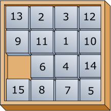
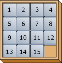
Figure 1: Two configurations of the 15-puzzle (left picture © 2008 Theon, right picture © 2006 Booyabazooka; via Wikipedia)

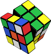
Figure 2: Rubik’s cube (© 2006 Booyabazooka; via Wikipedia)

More abstract kinds of reconfiguration problems abound in graph theory. For instance, suppose we are given a planar graph and two 4-colourings of that graph. Is it possible to transform the first 4-colouring into the second one, by recolouring one vertex at a time, and never using more than 4 colours? Taking any two different 4-colourings of the complete graph $K_{4}$ shows that the answer is not always yes. But what would happen if we allowed a fifth colour? And whereas it is easy to see what the situation is with two 4-colourings of $K_{4}$, how hard is it to decide in general if two given 4-colourings of some planar graph can be transformed from one to the other by recolouring one vertex at a time?

As a final (class of) example in this introduction we mention reconfiguration problems on satisfiability problems. Given some Boolean formula and two satisfying assignments of its variables, is it possible to transform one assignment into the other by changing the value of one variable at a time, but so that the formula remains TRUE during the whole sequence of transformations?

In this survey we concentrate on complexity considerations of transformation problems. In other words, we are interested in knowing how hard it is computationally to decide if the answer to some problem involving transformation is yes or no. More specifically, we will look at two types of those complexity question, which very roughly can be described as follows:

A-to-B-Path

• Description of a collection of feasible configurations;
  description of one or more transformations changing one configuration to another;
  description of two feasible configurations $A,B$.

• Is it possible to change configuration $A$ into configuration $B$ by a sequence of transformations in which each intermediate configuration is a feasible configuration as well?

Path-between-All-Pairs

• Description of a collection of feasible configurations;
  description of one or more transformations changing one configuration to another.

• Is it possible for any two feasible configurations $A,B$ to change configuration $A$ into configuration $B$ by a sequence of transformations in which each intermediate configuration is a feasible configuration as well?

Of course, there are many other questions that can be asked: how many steps does it take to go from one configuration to another? Which two configurations are furthest apart? Etc., etc. Many of these questions have been considered for particular problems, and where opportune we shall mention some of this work.

An alternative way to formulate this type of problem is by using the concept of a configuration graph. This is the graph that has as vertex set the collection of all possible feasible configurations, while two configurations are connected by an edge if there is a transformation changing one to the other. Note that nothing that we have said so far rules out the possibility that the transformation goes one way only, but in general we will assume that we can always go back and forth between configurations. This means the configuration graph can be taken to be an undirected graph.

Using the language of configuration graphs, the two general decision problems above can be rephrased as follows. Path-between-All-Pairs: is the configuration graph connected? A-to-B-Path: given two vertices (configurations) in the configuration graph, are they in the same component?

In most of this survey we will use fairly informal language. So we may use “step” or “move” instead of “transformation” (a one-step change). On the other hand, “transform configuration $A$ to configuration $B$”, “move from $A$ to $B$” or “go from $A$ to $B$” usually indicate a sequence of transformations.

1.1 A little bit on computational complexity

This survey cannot give a full definition of the complexity classes we will encounter, and we only give a general, intuitive, description of some of them. The interested reader can find all details in appropriate textbooks, such as Garey & Johnson [26] and Papadimitriou [46].

We assume the reader is familiar with the concept of decision problems (problems that have as answer either “yes” or “no”) and the complexity classes P, NP and coNP. We will also regularly encounter the class PSPACE. A decision problem is in PSPACE, or can be solved in polynomial space, if there exists an algorithm that solves the problem and that uses an amount of memory that is polynomial in the size of the input. The related non-deterministic complexity class NPSPACE is similarly defined as the class of decision problems for which there exists a non-deterministic algorithm that can recognise “yes”-instances of the problem using an amount of memory that is polynomial in the size of the input. For a non-deterministic algorithm we mean by recognising “yes”-instances that for every “yes”-instance (but for none of the “no”-instances) there is a possible run of the algorithm that finishes in finite time with a “yes” answer.

We obviously have $\text{{P}}\subseteq\text{{NP}}\cap\text{{coNP}}$ and $\text{{PSPACE}}\subseteq\text{{NPSPACE}}$, and a little bit of thought should convince the reader that we also have $\text{{NP}}\cup\text{{coNP}}\subseteq\text{{PSPACE}}$. (Trial and error of all possible solutions of a problem in NP or coNP can be done in polynomial space.) For most of these inclusions it is unknown if they are proper inclusions or if the classes are in fact the same, leading to some of the most important problems in computer science (settling whether or not $\text{{P}}=\text{{NP}}$ is worth a million dollars [17]). The one exception is that we know that PSPACE and NPSPACE are in fact the same by the celebrated theorem of Savitch [48].

Within each complexity class we can define so-called complete problems. Again, we refer to the appropriate textbooks for the precise definition; for us it is enough intuitively to assume that these are the “most difficult” problems in their class.

1.2 Computational complexity of reconfiguration problems

In order to be able to ask sensible questions (and obtain sensible answers) about the complexity of reconfiguration problems, we will make some assumptions regarding their properties. In particular, when describing the possible configurations, we will assume that these are not given as a full set of all configurations, but by some compact description. Otherwise, if the set of all possible configurations was part of the input, most decision problems about those configurations would trivially be possible in polynomial time because the input would be very large.

More precisely, we assume that an instance of the input contains an algorithm to decide if a candidate configuration really is feasible or not. Similarly, we are in general not interested in problems where the collection of possible transformations needs to be given (in the form of a list of all pairs that are related by the transformation). Instead, we assume that the input contains an algorithm to decide, given two configurations, whether or not we can get the second configuration from the first by a single transformation.

Regarding these algorithmic issues of the description of an instance of a configuration problem, we make the following assumptions:

• Deciding if a given possible configuration is a feasible configuration can be done in polynomial time.

• Given two feasible configurations, deciding if there is a transformation from the first to the second can be done in polynomial time.

Note that these assumptions guarantee that both of our general reconfiguration problems are in NPSPACE (hence in PSPACE by Savitch’s Theorem). The following is a non-deterministic algorithm for A-to-B-Path that would work in polynomial space, when required to decide if it is possible to have a sequence of transformations from configuration $A$ to configuration $B$:

• Given the initial configuration $A$, “guess” a next configuration $A_{1}$. Check that $A_{1}$ is indeed a feasible configuration and that there is transformation from $A$ to $A_{1}$. If $A_{1}$ is a valid next configuration, “forget” the initial configuration $A$ and replace it by $A_{1}$.

• Repeat the step above until the target configuration $B$ has been reached.

If there is indeed a way to go from configuration $A$ to configuration $B$, then a sequence of correct guesses in the algorithm above will indeed recognise that, using a polynomial amount of space; while if there is no sequence of transformations from $A$ to $B$, then the algorithm will never finish. To extend the algorithm to the Path-between-All-Pairs problem, we just need to repeat this task for all possible pairs. This means systematically generating all pairs of candidate configurations, and testing those. Since each candidate configuration has a size that is polynomial in the size of the original input (as it can be tested in polynomial time whether or not a candidate configuration is feasible), this brute-force generation of all possible pairs of configurations and testing whether or not they are feasible and connected can be done in a polynomial amount of memory as well.

The fact that all problems we consider are “automatically” in PSPACE means that we are in particular interested in determining if a particular variant is in a more restricted class (P, NP), or if it is in fact PSPACE-complete.

A final property that all examples we look at will have is that the transformations are symmetric: if we can transform one configuration into another, then we can also go the other way round. There is no real reason why this symmetry should always be the case, it is just that most reconfiguration problems considered in the literature have this feature. In particular, the sliding token problems we look at in Section 4 could just as well be formulated for directed graphs, leading in general to directed reconfiguration problems.

2 Reconfiguration of satisfiability problems

A collection of interesting results regarding the reconfiguration of solutions of a given Boolean formula were obtained by Gopalan et al. [28, 29]. They considered the following general set-up. Given a Boolean formula $\varphi$ with $n$ Boolean variables, the feasible configurations are those assignments from $\{T,F\}^{n}$ that satisfy $\varphi$ (i.e., for which $\varphi$ gives the value TRUE); the allowed transformation is changing the value of exactly one of the variables.

The collection of all possible assignments, together with edges added between those pairs that differ in exactly one variable, gives us the structure of the (graph of the) $n$-dimensional hypercube. This means that the configuration graph for a Boolean formula reconfiguration problem is the induced subgraph of the hypercube induced by the satisfying assignments. It is this additional structure that should give hope of a better understanding of this type of reconfiguration problem.

The first to analyse the connectivity properties of the configuration graphs of this type of problem were Gopalan et al. [28, 29]. To describe their results, we need a few more definitions.

A logical relation $R$ is a subset of $\{T,F\}^{k}$, where $k$ is the arity of $R$. For instance, if $R_{1/3}=\{TFF,FTF,FFT\}$, then $R_{1/3}(x_{1},x_{2},x_{3})$ is TRUE if and only if exactly one of $x_{1},x_{2},x_{3}$ is $T$. For $\mathcal{S}$ a finite set of logical relations, a CNF($\mathcal{S}$)-formula over a set of variables $V=\{x_{1},x_{2},\ldots,x_{n}\}$ is a finite conjunction $C_{1}\wedge C_{2}\wedge\dots\wedge C_{m}$ of clauses built using relations from $\mathcal{S}$, variables from $V$, and the constants $T$ and $F$. Hence each $C_{i}$ is an expression of the form $R(\xi_{1},\xi_{2},\ldots,\xi_{k})$, where $R$ is a relation of arity $k$, and each $\xi_{j}$ is a variable from $V$ or one of the Boolean constants $T,F$. The satisfiability problem Sat($\mathcal{S}$) associated with a finite set of logical relations $\mathcal{S}$ asks: given a CNF($\mathcal{S}$)-formula $\varphi$, is it satisfiable?

As an example, if we use the relation $R_{1/3}$ as above, and set $\mathcal{S}_{1/3}=\{R_{1/3}\}$, then CNF($\mathcal{S}_{1/3}$) consists of Boolean expressions of the form

$$\varphi=(x_{i}\vee x_{j}\vee x_{k})\wedge(x_{i^{\prime}}\vee x_{j^{\prime}}\vee x_{k^{\prime}})\wedge\cdots.$$

Finally, such an expression $\varphi$ is true for some assignment from $\{T,F\}$ to the variables if and only if each clause $x_{i}\vee x_{j}\vee x_{k}$ has exactly one variable that is $T$. The satisfiability problem Sat($\mathcal{S_{1/3}}$) is known as Positive-1-In-3-Sat; a decision problem that is NP-complete [49].

Another, better known, example is obtained by taking $\mathcal{S}_{2}=\{\,\{TF,FT,TT\},$ $\{FF,FT,TT\},\,\{FF,TF,FT\}\,\}$. Here the relation $R=\{TF,FT,TT\}$ indicates that $R(x_{1},x_{2})$ is TRUE when at least one of $x_{1},x_{2}$ is $T$, hence it represents clauses of the form $x_{1}\vee x_{2}$. Similarly, $\{FF,FT,TT\}$ represents clauses $\neg x_{1}\vee x_{2}$, and $\{FF,TF,FT\}$ represents clauses $\neg x_{1}\vee\neg x_{2}$. We see that CNF($\mathcal{S}_{2}$) is exactly the set of Boolean expressions that can be formulated with clauses that are disjunctions of two literals. (A literal is one of $x_{1}$ or $\neg x_{i}$ for a variable $x_{i}\in V$.) We call such a formula a 2-CNF-formula.

Similarly, the 3-CNF-formulas are exactly those formulas whose set of relations is $\mathcal{S}_{3}=\{R_{0},R_{1},R_{2},R_{3}\}$, where

$$\begin{array}[]{@{}c@{}}R_{0}\>=\>\{T,F\}^{3}\setminus\{FFF\},\quad R_{1}\>=\>\{T,F\}^{3}\setminus\{TFF\},\\ R_{2}\>=\>\{T,F\}^{3}\setminus\{TTF\},\quad R_{3}\>=\>\{T,F\}^{3}\setminus\{TTT\}.\end{array}$$

Note that this also means that Sat($\mathcal{S}_{2}$) and Sat($\mathcal{S}_{3}$) are equivalent to the well-known 2-SAT and 3-SAT decision problems, respectively.

Schaefer [49] proved a celebrated dichotomy theorem about the complexity of Sat($\mathcal{S}$): for certain sets $\mathcal{S}$ (nowadays called Schaefer sets), Sat($\mathcal{S}$) is solvable in polynomial time; while for all other sets $\mathcal{S}$ the problem is NP-complete.

In [28, 29], the following two decision problems are considered for given $\mathcal{S}$.

st-Conn($\mathcal{S}$)

• A CNF($\mathcal{S}$)-formula $\varphi$, and two satisfying assignments s and t of $\varphi$.

• Is there a path between s and t in the configuration graph of solutions of $\varphi$?

Conn($\mathcal{S}$)

• A CNF($\mathcal{S}$)-formula $\varphi$.

• Is the configuration graph of solutions of $\varphi$ connected?

The key concept for these problems appears to be that of a tight set of relations $\mathcal{S}$ – see [28, 29] for a precise definition of this concept. Here we only note that every Schaefer set is tight.

Theorem 2.1 (Gopalan et al. [28, 29])

Let $\mathcal{S}$ be a finite set of logical relations.

(a)If $\mathcal{S}$ is tight, then st-Conn($\mathcal{S}$) is in P; otherwise, st-Conn($\mathcal{S}$) is PSPACE-complete.

(b)If $\mathcal{S}$ is tight, then Conn($\mathcal{S}$) is in coNP; if it is tight but not Schaefer, then it is coNP-complete; otherwise, it is PSPACE-complete.

(c)If every relation $R$ in $\mathcal{S}$ is the set of solutions of a 2-CNF-formula, then Conn($\mathcal{S}$) is in P.

Major parts of the proof of Theorem 2.1 in [28, 29] follow a similar strategy to the proof of Schaefer’s Theorem in [49]. Given a set of relations $\mathcal{S}$, a $k$-ary relation $R$ is expressible from $S$ if there is a CNF($\mathcal{S}$)-formula $\varphi(x_{1},\ldots,x_{k},z_{1},\ldots,z_{m})$ such that $R$ coincides with the set of all assignments to $x_{1},\ldots,x_{k}$ that satisfy $(\exists z_{1})\,\cdots\,(\exists z_{m})\,\varphi(x_{1},\ldots,x_{k},z_{1},\ldots,z_{m})$. Then the essential part of the proof of Schaefer’s Theorem is that if a set $\mathcal{S}$ of relations is not-Schaefer, then every logical relation is expressible from $\mathcal{S}$.

The authors in [28, 29] extend the concept of expressibility to structurally expressibility. Informally, a relation $R$ is structurally expressible from a set of relations $\mathcal{S}$, if $R$ is expressible using some CNF($\mathcal{S}$)-formula $\varphi(x_{1},\ldots,x_{k},z_{1},\ldots,z_{m})$ and if the subgraph of the hypercube formed by the satisfying assignments of $\varphi$ has components that ‘resemble’ the components formed by the subgraph of the hypercube of the relations in $R$. The crucial result is that if a set of relations $\mathcal{S}$ is not tight, then every logical relation is structurally expressible from $\mathcal{S}$. Although the outline of this (part of the) proof is very similar to the outline of the corresponding part of Schaefer’s Theorem, the actual proof is considerably more involved.

Additionally, the following results on the structure of the configuration graphs of the solutions of different CNF($\mathcal{S}$)-formula are obtained in [28, 29].

Theorem 2.2 (Gopalan et al. [28, 29])

Let $\mathcal{S}$ be a finite set of logical relations.

(a)If $\mathcal{S}$ is tight, then for any CNF($\mathcal{S}$)-formula $\varphi$ with $n$ variables, if two satisfying assignments s and t of $\varphi$ are connected by a path, then the number of transformations needed to go from s to t is $O(n)$.

(b)If $\mathcal{S}$ is not tight, then there exists an exponential function $f(n)$ such that for every $n_{0}$ there exists a CNF($\mathcal{S}$)-formula $\varphi$ with $n\geq n_{0}$ variables and two satisfying assignments s and t of $\varphi$ that are connected by a path, but where the number of transformations needed to go from s to t is at least $f(n)$.

Regarding the result in Theorem 2.1 (b), in their original paper [28] the authors in fact conjectured a trichotomy for the complexity of Conn($\mathcal{S}$), conjecturing that if $\mathcal{S}$ is Schaefer, then Conn($\mathcal{S}$) is actually in P. They showed this conjecture to be true for particular types of Schaefer set (see Theorem 2.1 (b) for one example). The conjecture was disproved (assuming $\text{{P}}\neq\text{{NP}}$) by Makino et al. [42], who found a set of Schaefer relations for which Conn($\mathcal{S}$) remains coNP-complete. In the updated version [29], a modified trichotomy conjecture for the complexity of Conn($\mathcal{S}$) is formulated.

3 Reconfiguration of graph colourings

Reconfiguration of different kinds of graph colourings is probably one of the best studied examples of reconfiguration problems. We will look at some particular variants. The required background in the basics of graph theory can be found in any textbook on graph theory, such as Bondy & Murty [8] or Diestel [22].

3.1 Single-vertex recolouring of vertex colourings

Recall that a $k$-colouring of a graph $G=(V,E)$ is an assignment $\varphi:V\rightarrow\{1,\ldots,k\}$ such that $\varphi(u)\neq\varphi(v)$ for every edge $uv\in E$. A graph is $k$-colourable if it has a $k$-colouring.

We start by considering the case where we are allowed to recolour one vertex at a time, while always maintaining a valid $k$-colouring. We immediately get the following two reconfiguration problems, for a fixed positive integer $k$.

$k$-Colour-Path

• A graph $G$ together with two $k$-colourings $\alpha$ and $\beta$.

• Is it possible to transform the first colouring $\alpha$ into the second colouring $\beta$ by recolouring one vertex at a time, while always maintaining a valid $k$-colouring?

$k$-Colour-Mixing

• A graph $G$.

• Is it possible, for any two $k$-colourings of $G$, to transform the first one into the second one by recolouring one vertex at a time, while always maintaining a valid $k$-colouring?

Let us call a graph $G$ $k$-mixing if the answer to the second decision problem is yes. The use of the work “mixing” in this context derives from its relation with work on rapid mixing of Markov chains to sample combinatorial configurations; we say more about this in the final Section 5.

A variant of graph colouring is list-colouring. Here we assume that each vertex $v$ of a graph $G$ has its own list $L(v)$ of colours. An $L$-colouring of the vertices is an assignment $\varphi:V\longrightarrow\bigcup_{v\in V}L(v)$ such that $\varphi(v)\in L(v)$ for each vertex $v\in V$, and $\varphi(u)\neq\varphi(v)$ for every edge $uv\in E$. We call such a colouring a $k$-list-colouring if each list $L(v)$ contains at most $k$ colours.

Regarding a transformation of a list-colouring, we use the obvious choice: recolour one vertex at a time, where the new colour must come from the list for that vertex list. With all this, we say that a graph $G$ with list assignments $L$ is $L$-list-mixing if for every two $L$-colourings $\alpha$ and $\beta$, we can transform $\alpha$ into $\beta$ by recolouring one vertex at a time, while always maintaining a valid $L$-colouring.

We also have two related decision problems.

$k$-List-Colour-Path

• A graph $G$, list assignments $L(v)$ with $|L(v)|\leq k$ for each vertex $v\in V$, and two $L$-colourings $\alpha$ and $\beta$.

• Is it possible to transform the first colouring $\alpha$ into the second colouring $\beta$ by recolouring one vertex at a time, while always maintaining a valid $L$-colouring?

$k$-List-Colour-Mixing

• A graph $G$ and list assignments $L(v)$ with $|L(v)|\leq k$ for each vertex $v\in V$.

• Is $G$ $L$-list-mixing?

Before we look in some detail at what is known about the decision problems defined in this subsection, we give some other results on (list-)mixing. The following result has been obtained independently several times, but the first instance appears to be in (preliminary versions) of Dyer et al. [23]. The degeneracy $\mathop{\operator@font deg}(G)$ of a graph $G$ is the minimum integer $d$ so that every subgraph of $G$ has a vertex of degree at most $d$. In other words, $\mathop{\operator@font deg}(G)$ is the maximum, over all subgraphs $H$ of $G$, of the minimum degree of $H$.

Theorem 3.1 (Dyer et al. [23])

For any graph $G$, if $k\geq\mathop{\operator@font deg}(G)+2$, then $G$ is $k$-mixing. In fact, $G$ is $L$-list-mixing for any list assignment $L$ such that $|L(v)|\geq\mathop{\operator@font deg}(G)+2$ for all $v\in V$.

• We only prove the $k$-mixing statement; the proof of the list version is essentially the same.

  We use induction on the number of vertices of $G$. The result is obviously true for the graph with one vertex, so suppose $G$ has at least two vertices. Let $v$ be a vertex with degree at most $\mathop{\operator@font deg}(G)$, and consider $G^{\prime}=G-v$. Note that $\mathop{\operator@font deg}(G^{\prime})\leq\mathop{\operator@font deg}(G)$, hence we also have $k\geq\mathop{\operator@font deg}(G^{\prime})+2$, and by induction we can assume that $G^{\prime}$ is $k$-mixing.

  Take two $k$-colourings $\alpha$ and $\beta$ of $G$, and let $\alpha^{\prime},\beta^{\prime}$ be the $k$-colourings of $G^{\prime}$ induced by $\alpha,\beta$. Since $G^{\prime}$ is $k$-mixing, there exists a sequence $\alpha^{\prime}=\gamma^{\prime}_{0},\gamma^{\prime}_{1},\ldots,\gamma^{\prime}_{N}=\beta^{\prime}$ of $k$-colourings of $G^{\prime}$ so that two consecutive colourings $\gamma^{\prime}_{i-1},\gamma^{\prime}_{i}$, $i=1,\ldots,N$, differ in the colour of one vertex, say $v_{i}$. Set $c_{i}=\gamma^{\prime}_{i}(v_{i})$, the colour of $v_{i}$ after recolouring. We now try to take the same recolouring steps to recolour $G$, starting from $\alpha$. If for some $i$ it is not possible to recolour $v_{i}$, this must be because $v_{i}$ is adjacent to $v$ and $v$ at that moment has colour $c_{i}$. But because  $v$ has degree at most $\mathop{\operator@font deg}(G)\leq k-2$, there is a colour $c\neq c_{i}$ that does not appear on any of the neighbours of $v$. Hence we can first recolour $v$ to $c$, then recolour $v_{i}$ to $c_{i}$, and continue.

  In this way we find a sequence of $k$-colourings of $G$, starting at $\alpha$, and ending in a colouring in which all the vertices except possibly $v$ will have the same colour as in $\beta$. But then, if necessary, we can do a final recolouring of $v$ to give it the colour from $\beta$, completing the proof.       $\square$

Theorem 3.1 is best possible, as can be seen, e.g., by the complete graphs $K_{n}$ and trees. (For a tree $T$ we have $\mathop{\operator@font deg}(T)=1$, while it is trivial to check that a graph with at least one edge is never 2-mixing.) Constructions of graphs that are $k$-mixing for specific values of $k$, and not for other values, can be found in Cereceda et al. [13].

Since the degeneracy $\mathop{\operator@font deg}(G)$ of a graph $H$ is clearly at most the maximum degree $\Delta(G)$, Theorem 3.1 immediately means that for $k\geq\Delta(G)+2$, $G$ is $k$-mixing, as already noted by Jerrum [35, 36].

An interesting result that is related to Theorem 3.1 was proved by Choo & MacGillivray [16]. They proved that if $k\geq\mathop{\operator@font deg}(G)+3$, then the configuration graph (formed by all $k$-colourings with edges between colourings that differ in the colour on one vertex) is Hamiltonian. In other words, for those $k$ we can start at any $k$-colouring of $G$ and then there is a sequence of single-vertex recolourings so that every other $k$-colouring appears exactly once, ending with the original starting colouring.

When $k\geq\mathop{\operator@font deg}(G)+2$, the proof of Theorem 3.1 provides an algorithm to find a sequence of transformations between any two $k$-colourings of $G$. But the best upper bound on the number of steps that can be obtained from the proof is exponential in the number of vertices of $G$. No graph is known for which such an exponential number of steps is necessary. In fact the following is conjectured in Cereceda [12].

Conjecture 3.2 (Cereceda [12])

For a graph $G$ on $n$ vertices and integer $k\geq\mathop{\operator@font deg}(G)+2$, any two $k$-colourings of $G$ can be transformed from one into the other using $O(n^{2})$ single-vertex recolouring steps.

If true, the value $O(n^{2})$ in Conjecture 3.2 would be best possible. Some weaker versions of the conjecture were proved in [12].

Theorem 3.3 (Cereceda [12])

Conjecture 3.2 is true under the stronger assumptions $k\geq 2\mathop{\operator@font deg}(G)+1$ or $k\geq\Delta(G)+2$.

Theorem 3.3 means that Conjecture 3.2 is true if $G$ is a tree (then $\mathop{\operator@font deg}(G)+2=3=2\mathop{\operator@font deg}(G)+1$) or if $G$ is regular (in which case $\mathop{\operator@font deg}(G)=\Delta(G)$).

Note that Theorem 3.1 has algorithmic consequences if we restrict the decision problems to classes of graph in which each graph has degeneracy at most some fixed upper bound. For instance, as planar graphs have degeneracy at most 5, we obtain that 7-Colour-Mixing and 7-Colour-Path restricted to planar graphs are trivially in P, as the answer is always “yes”.

We now return to the recolouring complexity problems introduced earlier in this subsection. The following are some results that are known about those problems.

Theorem 3.4

(a)If $k=2$, then $k$-Colour-Path and $k$-Colour-Mixing are in P.

(b)If $k=3$, then $k$-Colour-Path is in P; while $k$-Colour-Mixing is coNP-complete (Cereceda et al. [14, 15]).

(c)For all $k\geq 4$, $k$-Colour-Path is PSPACE-complete (Bonsma and Cereceda [9]).

Theorem 3.5

(a)If $k=2$, then $k$-List-Colour-Path and $k$-List-Colour-Mixing are in P.

(b)For all $k\geq 3$, $k$-List-Colour-Path is PSPACE-complete (Bonsma and Cereceda [9]).

We already noted that the claims in Theorem 3.4 (a) are trivial: if we have only two colours, then the end-vertices of any edge can never be recoloured.

The results in Theorem 3.4 (b) are clearly the odd ones among the list of results above. The proof in [14] of the coNP-completeness of 3-Colour-Mixing uses the concept of folding: given two non-adjacent vertices $u$ and $v$ that have a common neighbour, a fold on $u$ and $v$ is the identification of $u$ and $v$ (together with removal of any double edges produced). We say a graph $G$ is foldable to $H$ if there exists a sequence of folds that transforms $G$ to $H$. Folding of graphs, and its relation to vertex colouring, has been studied before, see for instance [18].

Combining observations from [13] for non-bipartite 3-colourable graphs, with the structural characterisation of bipartite graphs that are not 3-mixing in [14], gives the following.

Theorem 3.6 (Cereceda et al. [13, 14])

Let $G$ be a connected 3-colourable graph. Then $G$ is not 3-mixing if and only if $G$ is foldable to the 3-cycle $C_{3}$ or the 6-cycle $C_{6}$.

It is easy to see that every non-bipartite 3-colourable connected graph can be folded to $C_{3}$, so the interesting part of this theorem is the characterisation of bipartite non-3-mixing graphs as being foldable to $C_{6}$. In a sense, the theorem shows that $C_{3}$ and $C_{6}$ are the ‘minimal’ graphs that are not 3-mixing.

Theorem 3.5 (b) is not explicitly given in Bonsma and Cereceda [9], but follows from the proof of Theorem 3.4 (c) in that paper.

The results that 2-List-Colour-Path and 2-List-Colour-Mixing can be done in polynomial time can be proved directly with some effort. But it is easy to see that in fact any 2-list-colouring problem can be reduced to a Boolean 2-CNF-formula. For each vertex $v$ and colour $c\in L(v)$, introduce a Boolean variable $x_{v,c}$. Then for each vertex $v$ with $L(v)=\{c,d\}$ we add a clause $x_{v,c}\vee x_{v,d}$; while for each edge $uv$ and colour $c\in L(u)\cap L(v)$ we add a clause $(\neg x_{u,c})\vee(\neg x_{v,c})$. We can now use the results that checking the connectivity of the solution space of a 2-CNF-formula is in P, see Theorem 2.1 (c).

As well as the computational complexity of some of the recolouring problems, we also know something about the number of recolourings we might need.

Theorem 3.7

(a)For a graph $G$ on $n$ vertices, if two 3-colourings of $G$ can be connected by a sequence of single-vertex recolourings, then this can be done in $O(n^{2})$ steps (Cereceda et al. [15]).

(b)For any $k\geq 3$ there exists an exponential function $f(n)$ such that for every $n_{0}$, there exists a graph $G$ on $n\geq n_{0}$ vertices, an assignment $L$ of lists of size $k$ to the vertices of $G$, and two $L$-colourings $\alpha$ and $\beta$ of $G$, such that we can transform $\alpha$ into $\beta$ by recolouring one vertex at a time, but where the number of recolourings required is at least $f(n)$ (Bonsma and Cereceda [9]).

(c)For any $k\geq 4$, the result in (b) also holds for ordinary $k$-colouring recolourings.

The bound $O(n^{2})$ in Theorem 3.7 (a) is best possible.

Two remaining questions are the complexity class of $k$-Colour-Mixing for $k\geq 4$ and $k$-List-Colour-Mixing for $k\geq 3$. In view of the fact that $k$-Colour-Path and $k$-List-Colour-Path for those values of $k$ are PSPACE-complete, one would expect the mixing variants to have a similar complexity. On the other hand, since the coNP-completeness of 3-Colour-Mixing is obtained by a particular structure that needs to be present in a graph to fail to be 3-mixing, a similar graph-structural condition for mixing with more colours might well be possible.

In view of the results that many of the recolouring problems are not in P (assuming that $\text{{P}}\neq\text{{NP}}$), it is interesting to find restricted instances for which the recognition problems are in P. A natural choice for a graph class where one expects this to happen is the class of bipartite graphs, since many colouring problems are trivial in that class. Surprisingly, restricting the input of the decision problems to just bipartite graphs does not change any of the results in Theorems 3.4–3.7. A restriction to planar graphs has more surprising results, as expressed in the final result of this subsection.

Theorem 3.8

(a)When restricted to planar graphs, 3-Colour-Mixing becomes polynomial (Cereceda et al. [14]).

(b)When restricted to planar graphs, $k$-Colour-Path for $4\leq k\leq 6$ and $k$-List-Colour-Path for $3\leq k\leq 6$ remain PSPACE-complete (Bonsma and Cereceda [9]).
Both decision problems are in P for $k\geq 7$ when restricted to planar graphs.

(c)When restricted to bipartite planar graphs, $k$-Colour-Path for $k=4$ and $k$-List-Colour-Path for $3\leq k\leq 4$ remain PSPACE-complete (Bonsma and Cereceda [9]).
Both decision problems are in P for $k\geq 5$ when restricted to bipartite planar graphs.

The results that $k$-Colour-Path and $k$-List-Colour-Path are polynomial for planar or bipartite planar graphs and larger $k$, follows directly from upper bounds for the degeneracy for those graphs and Theorem 3.1.

3.2 Kempe chain recolouring

Given a $k$-colouring $\varphi$ of a graph $G$, a Kempe chain is a connected component of the subgraph of $G$ induced by the vertices coloured with one of two give colours. In other words, if $c_{1},c_{2}$ are two different colours, and $W\subseteq V$ is the collection of vertices coloured either $c_{1}$ or $c_{2}$, then a Kempe chain is a connected component of the induced subgraph of $G$ with vertex set $W$. By a Kempe chain recolouring we mean switching the two colours on a Kempe chain. Kempe chains and Kempe chain recolouring have been essential concepts in the proofs of many classical results on colouring, such as the Four Colour Theorem from Appel & Haken [2, 4, 3] and Vizing’s Edge-Colouring Theorem [54].

Notice that a Kempe chain recolouring is a generalisation of the single-vertex recolouring transformation from the previous subsection, since such a recolouring corresponds to a Kempe chain recolouring on a Kempe chain consisting of just one vertex. Let us call a graph $G$ $k$-Kempe-mixing if it is possible, for any two $k$-colourings of $G$, to transform the first one into the second one by a sequence of Kempe chain recolourings.

From the observation above, we see that if a graph is $k$-mixing, then it certainly is $k$-Kempe-mixing. But the reverse need not be true. For instance, it has been observed many times that a bipartite graph is $k$-Kempe-mixing for any $k\geq 2$ [11, 25, 45], whereas for any $k\geq 2$ there exist bipartite graphs that are not $k$-mixing [13]. Furthermore, a simple modification of the proof of Theorem 3.1 shows that for any graph $G$, if $k\geq\mathop{\operator@font deg}(G)+1$, then $G$ is $k$-Kempe-mixing, as was already proved by Las Vergnas & Meyniel [39].

Very little is known about the complexity of determining if a graph is $k$-Kempe-mixing. The same holds for the ‘path’ version of the problem (determining if two given $k$-colourings can be transformed into one another by a sequence of Kempe chain recolourings). Intuitively, there appear to be at least two reasons why Kempe chain recolouring is so much harder to analyse than single-vertex recolouring. Firstly, for any $k$-colouring of a graph it is always possible to perform Kempe chain recolourings. This is different from single-vertex recolouring, where it might not be possible to recolour any vertex at all (if all vertices have all colours different from their own appearing on a neighbour). This kind of ‘frozen’ colourings is essential in many of the analyses and results on single-vertex recolourings. Secondly, whereas a single-vertex recolouring has only a ‘local’ effect, a Kempe chain can affect many vertices throughout the graph.

The following are some results for planar graphs.

Theorem 3.9

(a)Every planar graph is 5-Kempe-mixing (Meyniel [44]).

(b)If $G$ is a 3-colourable planar graph, then $G$ is 4-Kempe-mixing (Mohar [45]).

The results in the theorem are best possible in the sense that the number of colours cannot be reduced in either statement [45].

As we have observed earlier, for the single-vertex recolouring problem, the smallest graph that is not 3-mixing is the triangle $C_{3}$, while the smallest bipartite graph that is not 3-mixing is the 6-cycle $C_{6}$. These graphs are essential in the proof that 3-Colour-Mixing is coNP-complete. The smallest graph that is not 3-Kempe-mixing is the 3-prism $K_{3}\mathop{\Box}K_{2}$ (see Figure 3).

Figure 3: The 3-prism with two 3-colourings that are not related by Kempe chains

It is easy to check that any Kempe chain recolouring in these two colourings will only result in renaming the two colours involved in the Kempe chain, but never changes the structure. It is unknown if the 3-prism is in some way a ‘minimal’ graph that is not 3-Kempe mixing, or if it is the only one. Neither is it obvious what subgraph relation we should use (like ‘foldable’ for the single-vertex recolouring problem) when talking about ‘minimal’ for Kempe-mixing.

Kempe chains have also been used extensively in the analysis of edge-colourings of graphs. Recall that a $k$-edge-colouring of a graph $G=(V,E)$ is an assignment $\varphi:E\rightarrow\{1,\ldots,k\}$ such that $\varphi(e)\neq\varphi(f)$ for any two edges $e,f$ that share a common end-vertex. Similar to vertex-colourings, a Kempe chain in an edge-coloured graph is a component of the subgraph formed by the edges coloured with one of two given colours. Note that in this case every Kempe chain is a path or an even length cycle, and a recolouring is again just switching the colours on the chain. Call a graph $G$ $k$-Kempe-edge-mixing if it is possible for any two $k$-edge-colourings of $G$ to transform the first one into the second one by a sequence of Kempe chain recolourings.

Kempe chains on edge-colourings are instrumental in most (if not all) proofs of Vizing’s Theorem [54] that a simple graph with maximum degree $\Delta$ has an edge-colouring using at most $\Delta+1$ colours. Hence it is not surprising that results on $k$-Kempe-edge mixing are related to this constant as well.

Theorem 3.10 (Mohar [45])

(a)If a simple graph $G$ can be edge-coloured with $k$ colours, then $G$ is $(k+2)$-Kempe-edge-mixing.

(b)If $G$ is a simple bipartite graph with maximum degree $\Delta$, then $G$ is $(\Delta+1)$-Kempe-edge-mixing.

It is unknown if Theorem 3.10 (a) is best possible, nor if the condition that the graph be bipartite in part (b) is necessary. A strongest possible result would be for any simple graph with maximum degree $\Delta$ to be $(\Delta+1)$-Kempe-edge-mixing.

4 Moving tokens on graphs

The 15-puzzle can be considered as a problem involving moving tokens around a given graph, where a token can be moved along an edge to an empty vertex. So the two configurations in Figure 1 can also be drawn as in Figure 4.

Figure 4: Two configurations of the 15-puzzle on the $4\times 4$ grid

Looking at the 15-puzzle in this way immediately suggests all kind of generalisations. An obvious generalisation is to play the game on different graphs. But we can also change the number of tokens, or the way the tokens are labelled. In this section we consider some of the variants that have been studied in the literature.

4.1 Labelled tokens without restrictions

There is an obvious generalisation of the 15-puzzle. For a given graph on $n$ vertices, place $n-1$ tokens labelled 1 to $n-1$ on different vertices. The allowed moves are “sliding” a token along an edge onto the unoccupied vertex. The central question is if each of the $n!$ possible token configurations can be obtained from one another by a sequence of token moves. A complete answer to this was given in Wilson [57]. For a given graph $G$ on $n$ vertices, he defines the puzzle graph $\mathop{\operator@font puz}(G)$ as the graph that has as vertex set all possible placements of the $n-1$ tokens on $G$, and two configurations are adjacent if they can be obtained from one another by a single move.

Theorem 4.1 (Wilson [57])

Let $G$ be a 2-connected graph on $n\geq 3$ vertices. Then $\mathop{\operator@font puz}(G)$ is connected, except in the following cases:

(a)$G$ is a cycle on $n\geq 4$ vertices (in which case $\mathop{\operator@font puz}(G)$ has $(n-2)!$ components);

(b)$G$ is a bipartite graph different from a cycle (then $\mathop{\operator@font puz}(G)$ has two components);

(c)$G$ is the graph $\theta_{0}$ in Figure 5 (then $\mathop{\operator@font puz}(G)$ has six components).

Figure 5: The exceptional graph $\theta_{0}$

The condition in Wilson’s theorem that the graph $G$ is 2-connected is necessary. It is obvious that for a non-connected graph $G$, $\mathop{\operator@font puz}(G)$ is never connected; while if $G$ has a cut-vertex $v$, then a token can never be moved from one component of $G-v$ to another component.

The proof of Theorem 4.1 in [57] is quite algebraic in nature. This is not surprising, since each token configuration can be considered as a permutation of $n$ labels (with the unoccupied vertex having the label ‘empty’). Within that context, a move is just a particular type of transposition involving two labels (one of them always being the ‘empty’ label). Although Wilson’s theorem is not formulated in algorithmic terms, it is easy to derive from it a polynomial time algorithm to decide if $\mathop{\operator@font puz}(G)$ is connected for a given input graph $G$.

Since Wilson’s work (and often independent of it), many generalisations have been considered in the literature. To describe these in some detail, we need some further notation. Instead of assuming that all tokens are different, we will assume that some tokens can be identical. So tokens come in certain types (other authors use colours for this), where tokens of the same type are considered indistinguishable (and hence swapping tokens of the same type will not lead to a different configuration). A collection of tokens can have $k_{1}$ tokens of type 1, $k_{2}$ tokens of type 2, etc. We denote such a typed set by $(k_{1},k_{2},\ldots,k_{p})$, so that $k_{1}+\dots+k_{p}$ is the total number of tokens. A repeated sequence of $p$ ones can be denoted as $1^{(p)}$.

Given a graph $G$ and token set $(k_{1},\ldots,k_{p})$, the puzzle graph $\mathop{\operator@font puz}(G;k_{1},\dots,k_{p})$ is the graph that has as vertex set all possible token placements on $G$ of $k_{1}$ tokens of type 1, $k_{2}$ tokens of type 2, etc., and two configurations are adjacent if they can be obtained from one another by a single move of a token to a neighbouring empty vertex. This means that if $G$ is a graph on $n$ vertices, then $\mathop{\operator@font puz}(G)\cong\mathop{\operator@font puz}(G;1^{(n-1)})$. We will always assume that if $G$ has $n$ vertices, then $k_{1}+\dots+k_{p}\leq n$ and $k_{1}\geq k_{2}\geq\dots\geq k_{p}\geq 1$.

A first generalisation of Wilson’s work, in which there may be fewer than $n-1$ tokens, was considered by Kornhauser et al. [38]. They showed that if $G$ is a graph on $n$ vertices, then for any two configurations from $\mathop{\operator@font puz}(G,1^{(p)})$, it can be decided in polynomial time if these two configurations are in the same component, i.e., if one configuration can be obtained from the other by a sequence of token moves. Additionally, they showed that if such a transformation is possible, the number of moves required is at most $O(n^{3})$, and the order of this bound is best possible.

This work was further extended to token configurations with types as above; first to trees by Auletta et al. [5], and later to general graphs by Goraly & Hassin [30]. Their results prove that for any graph $G$ and typed token set $(k_{1},\ldots,k_{p})$, given two configurations from $\mathop{\operator@font puz}(G;k_{1},\ldots,k_{p})$, it can be decided in linear time if one configuration can be obtained from the other. Notice that by the result for all tokens being different mentioned earlier, we immediately have that for a graph on $n$ vertices, more than $O(n^{3})$ token moves are never needed between two configurations.

The work mentioned in the previous paragraphs does not give an explicit characterisation of the puzzle graphs $\mathop{\operator@font puz}(G;k_{1},\ldots,k_{p})$ that are connected (i.e., where any two token configurations of the right type can be obtained from one another by a sequence of token moves). In order to describe such a characterisation, we need some further terminology regarding specific vertex-cut-sets in graphs. For a connected graph $G$, a separating path of size one in $G$ is a cut-vertex. A separating path of size two is a cut-edge $e=v_{1}v_{2}$ so that both components of $G-e$ have at least two vertices. Finally, for $\ell\geq 3$, a separating path of size $\ell$ is a path $P=v_{1}v_{2}\ldots v_{\ell}$ in $G$, such that the vertices $v_{2},\ldots,v_{\ell-1}$ have degree two, $G-\{v_{2},\ldots,v_{\ell-1}\}$ has exactly two components, one containing $v_{1}$ and one containing $v_{\ell}$, and where both components have at least two vertices.

Theorem 4.2 (Brightwell et al. [10])

Let $G$ be a graph on $n\geq 3$ vertices and $(k_{1},\ldots,k_{p})$ be a token set, with $k_{1}+\dots+k_{p}\leq n$ and $k_{1}\geq k_{2}\geq\dots\geq k_{p}\geq 1$. Then $\mathop{\operator@font puz}(G;k_{1},\ldots,k_{p})$ is disconnected if and only if at least one of the following cases holds:

(a)$G$ is disconnected, and $p\geq 2$ or $k_{1}\leq n-1$;

(b)$p\geq 2$ and $k_{1}+\dots+k_{p}=n$;

(c)$G$ is a path and $p\geq 2$;

(d)$G$ is a cycle, $p=2$ and $k_{2}\geq 2$; or $G$ is a cycle and $p\geq 3$;

(e)$G$ is a 2-connected bipartite graph and the token set is $(1^{(n-1)})$;

(f)$G$ is the graph $\theta_{0}$ in Figure 5 and the token set is one of $(2,2,2)$, $(2,2,1,1)$, $(2,1,1,1,1)$, $(1^{(6)})$;

(g)$G$ has connectivity one and contains a separating path of size at least $n-(k_{1}+k_{2}+\dots+k_{p})$.

Note in particular that if $G$ is a 2-connected graph on $n$ vertices different from a cycle, and $(k_{1},\ldots,k_{p})$ is a token set with $k_{1}+\dots+k_{p}\leq n-2$, then $\mathop{\operator@font puz}(G;k_{1},\ldots,k_{p})$ is always connected.

It is possible to extend this theorem to a full characterisation of any two token configurations from any puzzle graph $\mathop{\operator@font puz}(G;k_{1},\ldots,k_{p})$ that are in the same component (hence extending the algorithmic results from Goraly & Hassin [30]). This rather technical and long result can also be found in [10].

The results mentioned above mean that it is quite straightforward to check if one can go from any given token configuration to any other one. So a next natural question is to ask if it is possible to find the shortest path, i.e., to find the minimum number of token moves required between two given token configurations in the same component of $\mathop{\operator@font puz}(G;k_{1},\ldots,k_{p})$. This leads to the following decision problem.

Shortest-Token-Moves-Sequence

• A graph $G$, a token set $(k_{1},\ldots,k_{p})$, two token configurations $\alpha$ and $\beta$ on $G$ of type $(k_{1},\ldots,k_{p})$, and a positive integer $N$.

• Is it possible to transform configuration $\alpha$ into configuration $\beta$ using at most $N$ token moves?

Theorem 4.3

Restricted to the case that the token sets are $(k)$ (i.e., all tokens are the same), Shortest-Token-Moves-Sequence is in P.

• We can assume that the given graph $G$ is connected. (Since two configurations can be transformed into one another if and only if this can be done for the configurations restricted to the components of the graph.) Given two token configurations $\alpha$ and $\beta$ of $k$ identical tokens on $G$, let $U=\{u_{1},\ldots,u_{k}\}$ be the set of vertices containing a token in $\alpha$, and $V=\{v_{1},\ldots,v_{k}\}$ be the same for $\beta$.

  Form a complete bipartite graph $K_{k,k}$ with parts $U$ and $V$. For each edge $e_{ij}=u_{i}v_{j}$, define the weight $w_{ij}$ of $e_{ij}$ as the length of the shortest path from $u_{i}$ to $v_{j}$ in $G$ (and denote by $P_{ij}$ such a shortest path in $G$). It is well-known that a minimum weight perfect matching in a weighted balanced complete bipartite graph can be found in polynomial time (for instance using the Hungarian method, see, e.g., Schrijver [50, Section 17.2]); let $M$ be such a minimum weight perfect matching.

  We can assume that $M=\{u_{1}v_{1},\ldots,u_{k}v_{k}\}$. Let $W$ be the total weight in $M$, i.e., the sum of the lengths of the paths $P_{ii}$, $i=1,\ldots,k$. It is obvious that any way to move the tokens from $U$ to $V$ will use at least $W$ steps. We will prove that in fact it is possible to do so using exactly $W$ steps. We use induction on $W$, observing that if $W=0$, then $U=V$, so $\alpha\equiv\beta$, and no tokens have to be moved.

  If $W>0$, then at least one element of $V$, say $v_{1}$, has no token on it in $\alpha$. If $V(P_{11})\cap U=\{u_{1}\}$, then we can just move the token from $u_{1}$ along $P_{11}$ to $v_{1}$, and are done by induction. So assume that $P_{11}$ contains some other elements from $U$. Take $u_{i}$ to be the element from $V(P_{11})\cap U$ nearest to $v_{1}$ on $P_{11}$. Define new paths $P^{\prime}_{1i}$ and $P^{\prime}_{i1}$ as follows. Let $P^{\prime}_{1i}$ be the path formed by going from $u_{1}$ along $P_{11}$ to $u_{i}$ and then continue along $P_{ii}$ to $v_{i}$; while $P^{\prime}_{i1}$ is just the path from $u_{i}$ along $P_{11}$ to $v_{1}$. It is clear that the sum of the lengths of $P^{\prime}_{1i}$ and $P^{\prime}_{i1}$ is the same as that sum for $P_{11}$ and $P_{ii}$, so we can replace $P_{11}$ and $P_{ii}$ by $P^{\prime}_{1i}$ and $P^{\prime}_{i1}$ to get another set of paths from $U$ to $V$ of minimum total length. But in this new collection of paths, we can just move $u_{i}$ along $P^{\prime}_{i1}$ to $v_{1}$, and then continue by induction.       $\square$

It was proved by Goldreich [27] that Shortest-Token-Moves-Sequence is NP-complete for the case Wilson considered, i.e., if all tokens are different. So somewhere between all tokens the same and all tokens different, the problem switches from being in P to being NP-complete. In fact, the change-over happens as soon as not all tokens are identical.

Theorem 4.4

Restricted to the case that the token sets are $(k-1,1)$ (i.e., there is one special token and all others are identical), Shortest-Token-Moves-Sequence is NP-complete.

It is possible to prove this using most of the ideas from the proof in Papadimitriou et al. [47] that ‘Graph-Motion-Planning-With-One-Robot’ is NP-complete. Motion planning of robot(s) on graphs is very closely related to transformations between token configurations on graphs. Except now there are some special tokens, the ‘robots’, that have to be moved from an initial position to a specific final position, while all other tokens are just ‘obstacles’, and their final position is not relevant. The full details of the proof of Theorem 4.4 will appear in Trakultraipruk [53].

4.2 Unlabelled Tokens with Restrictions

If we consider the token problems in the previous subsection for the case that all tokens are identical, then there is very little to prove. The puzzle graph $\mathop{\operator@font puz}(G;k)$ (with $k\leq|V(G)|$) is connected if and only if $k=|V(G)|$ or $G$ is connected. More specifically, two token configurations are in the same component of $\mathop{\operator@font puz}(G;k)$ if and only if they have the same number of tokens on each component of $G$. Even finding the minimum number of steps to go from one given configuration to another can be done in polynomial time. (Of course, this does not mean that questions about other properties of this kind of reconfiguration graphs cannot be interesting; see for instance Fabila-Monroy et al. [24].)

But the situation changes drastically if only certain positions of tokens are allowed. The following problem was studied in Hearn & Demaine [33]. Recall that a stable set in a graph is a set of vertices so that no two in the set are adjacent.

Stable-Sliding-Token-Configurations

• A graph $G$, and two token configurations on $G$ using identical tokens so that the set of occupied vertices for both configurations forms a stable set in $G$.

• Is it possible to transform the first given configuration into the second one by a sequence of moves of one token along an edge, and such that in every intermediate configurations the set of occupied vertices is a stable set?

Theorem 4.5 (Hearn & Demaine [33])

The problem Stable-Sliding-Token-Configurations is PSPACE-complete,even when restricted to planar graphs with maximum degree three.

The proof of this theorem in [33] (and many other results in that paper) rely on a powerful general type of problem that seems to be very suitable for complexity theoretical reductions. A non-deterministic constraint logic machine (NCL machine) consists of an undirected graph, together with assignments of non-negative integer weights to its edges and its vertices. A feasible configuration of an NCL machine is an orientation of the edges such that the sum of incoming edge-weights at each vertex is at least the weight of that vertex. A move is nothing other than reversing the orientation of one edge, guaranteeing that the resulting orientation is still a feasible configuration.

The following is a natural reconfiguration question for NCL machines.

NCL-Configuration-to-Edges

• An NCL machine, a feasible configuration on that machine, and a specific edge of the underlying graph.

• Is there a sequence of moves such that all intermediate configurations are feasible, and ending in a feasible configuration in which the specified edge has its orientation reversed?

Theorem 4.6 (Hearn & Demaine [33])

The problem NCL-Configuration-to-Edges is PSPACE-complete, even when restricted to NCL machines in which the underlying graph is planar, all vertices have degree three, all edge-weights are 1 or 2, and all vertex weights are 2.

We return to moving tokens configuration problems. Note that in the Stable-Sliding-Token-Configurations problem, the graph has a ‘double’ role: it determines both the allowed configurations (stable vertex sets) and the allowed moves (sliding along an edge). A natural next question would be what happens when one of these constraints imposed by the graph is removed. We have already seen that if we remove the constraint that the configurations must be stable sets, then the problem becomes easy. But the situation is different if we remove the constraint that token movement must happen along an edge.

Stable-Set-Reconfiguration

• A graph $G$, and two token configurations on $G$ using identical tokens so that the set of occupied vertices for both configurations forms a stable set in $G$.

• Is it possible to transform the first given configuration into the second one by a sequence of moves of one token at each step, where a token can move from any vertex to any other vacant one, and so that in every intermediate configuration the set of occupied vertices is a stable set?

Theorem 4.7 (Ito et al. [34])

The problem Stable-Set-Reconfiguration is PSPACE-complete, even when restricted to planar graphs with maximum degree three.

Since independent set problems are easily reduced to problems about cliques, vertex covers, etc., reconfiguration problems where the vertices occupied by a token form sets of this type are easily seen to be PSPACE-complete as well. See Ito et al. [34] for more details.

For some other types of sets formed by occupied vertices, the corresponding reconfiguration problems can become polynomial. A classical example of this is the following.

Theorem 4.8 (Cummins [20])

Let $G$ be a connected graph with positive weights on its edges. Then any minimum spanning tree of $G$ can be transformed into any other minimum spanning tree by exchanging one edge at a time, so that each intermediate configuration is a minimum spanning tree as well.

Note that the reconfiguration in Theorem 4.8 can be seen as a token reconfiguration problem by playing on the line graph of $G$. Similarly, the following problem is essentially Stable-Set-Reconfiguration played on line graphs.

Matching-Reconfiguration

• A graph $G$, and two matchings of $G$ (subgraphs of degree at most one).

• Is it possible to transform the first matching into the second one by a sequence of moves of one edge at a time, so that in every intermediate configuration the set of chosen edges forms a matching as well?

Theorem 4.9 (Ito et al. [34])

The problem Matching-Reconfiguration is in P.

Comparing the reconfiguration problems in this subsection that are PSPACE-complete with those that are in P, it is tempting to conjecture that if the related decision problem is NP-complete, then the reconfiguration problem is PSPACE-complete; whereas if the related decision problem is in P, then so is the reconfiguration problem. Such a connection is alluded to in Ito et al. [34]. Nevertheless, in earlier sections we have seen some examples that shows that such a direct connection is not true. For instance, it is NP-complete to decide if a graph is 3-colourable, but the single-vertex recolouring reconfiguration problem is in P, Theorem 3.4 (b).

We close this section with a simplified version of a question from Ito et al. [34]: is the Hamilton-Cycle-Reconfiguration problem (where two cycles are adjacent if they differ in two edges) PSPACE-complete?

5 Applications

Most reconfiguration problems are interesting enough for their own sake, and do not really need an application to justify their study. Nevertheless, many reconfiguration problems have applications or are inspired by problems in related areas. In this section we look at some of those applications and connections.

5.1 Sampling and counting

Randomness plays an important role in many parts of combinatorics and theoretical computer science. Indeed, results from probability theory have led to major developments in both fields. It is therefore unsurprising that researchers are often interested in obtaining random samples of particular combinatorial structures. For example, much attention has been devoted to the problem of sampling from an exponential number of structures (exponential in the size of the object over which the structures are defined) in time polynomial in this quantity. One of the reasons for this is that being able to sample almost uniformly from a set of combinatorial structures is enough to be able to approximately count such structures. See Jerrum [35] for an example illustrating the method in the context of graph colourings, and Jerrum [36] and Jerrum et al. [37] for full details.

The question of when the configuration graph of a reconfiguration problem is connected is quite old. In particular the configuration graph of the single-vertex recolouring method has been looked at, as a subsidiary issue, by researchers in the statistical physics community studying the ‘Glauber dynamics of an anti-ferromagnetic Potts model at zero temperature’. (See Sokal [51] for an introduction to the Potts model and its many relations to graph theory.) Associated with that research is the work on rapid mixing of Markov chains used to obtain efficient algorithms for almost uniform sampling of $k$-colourings of a given graph. We give a brief description of the basic ideas involved in these areas of research.

Quite often, the sampling is done via the simulation of an appropriately defined Markov chain. Here the important point is that the Markov chain should be rapidly mixing. This means, loosely speaking, that it should converge to a close approximation of the stationary distribution in time polynomial in the size of the problem instance. For a precise description of this concept and further details; see [36] again.

In the context of the particular Markov chain used for sampling $k$-colourings of a graph known as Glauber dynamics (originally defined for the anti-ferromagnetic Potts model at zero temperature) we have the following. For a particular graph $G$ and value of $k$, let us denote the Glauber dynamics for the $k$-colourings of $G$ by $\mathcal{M}_{k}(G)=(X_{t})_{t=0}^{\infty}$. The state space of $\mathcal{M}_{k}(G)$ is the set of all $k$-colourings of $G$, the initial state $X_{0}$ is an arbitrary colouring, and its transition probabilities are determined by the following procedure.

1. Select a vertex $v$ of $G$ uniformly at random.

2. Select a colour $c\in\{1,2,\ldots,k\}$ uniformly at random.

3. If recolouring vertex $v$ with colour $c$ yields a proper colouring, then set $X_{t+1}$ to be this new colouring; otherwise, set $X_{t+1}=X_{t}$.

The relation between $\mathcal{M}_{k}(G)$ and the single-vertex recolouring transformations is immediate. In particular, to be sure that every $k$-colouring can appear as some state of the Markov chain, we need that $G$ is $k$-mixing. Thus the fact that a graph is $k$-mixing is a necessary condition for its Glauber dynamics Markov chain to be rapidly mixing. (This explains the choice of terminology in Section 3.) On the other hand, if a graph is $k$-mixing it does not mean that its Glauber dynamics Markov chain is rapidly mixing. An example showing this is given by the stars $K_{1,m}$, which are $k$-mixing for any $k\geq 3$ (see Theorem 3.1) but whose Glauber dynamics is not rapidly mixing for $k\leq m^{1-\varepsilon}$, for fixed $\varepsilon>0$ (Łuczak & Vigoda [41]).

Let us point out that much of the work on rapid mixing of the Glauber dynamics Markov chain (as well as that on its many generalisations and variants) has concentrated on specific graphs, or on values of $k$ so large that $k$-mixing is guaranteed. Many applications in theoretical physics related to the Potts model are of particular interest for crystalline structures, leading to the many studies of the Glauber dynamics and its generalisations on very regular and highly symmetric graphs such as integer grids.

Similar to the single-vertex recolouring method, the Kempe chain recolouring method (see Subsection 3.2) has also been used to define a Markov chain on the set of all $k$-colourings of some graph. The corresponding approximate sampling algorithm is known as the Wang-Swendsen-Kotecký dynamics; see [55, 56].

Many reconfiguration problems we have considered so far can be used to define a Markov chain similar to the ones for vertex-colouring defined above. Again, for such a Markov chain to be a useful tool for almost uniform sampling and approximate counting, it is necessary that the configuration graph is connected, leading to questions considered in this survey.

5.2 Puzzles and games

We introduced the study of token configurations on graphs by looking at the classical 15-puzzle. But in fact, many puzzles and games can be described as reconfiguration problems. Following Demaine and Hearn [21] we use the term (combinatorial) puzzle if there is only one player, and use (combinatorial) game if there are two players. (So we ignore games with more than two players, or with no players (like Conway’s Game of Life).)

The puzzles we are interested in are of the following type: “Given some initial configuration and a collection of allowed moves, can some prescribed final configuration (or a final configuration from a prescribed set) be reached in a finite number of moves?” For a game the situation is somewhat more difficult, and several different variants can be described. A quite general one is: “Given some initial configuration, a starting player, a collection of allowed moves which the two players have to play alternately, and a collection of winning configurations for player 1, can player 1 force the game to always reach a winning configuration in a finite number of moves, no matter the moves player 2 chooses?” Another way to describe this question is: “Given the setup of the game and the initial situation, is there a winning strategy for player 1?”.

With these descriptions there is an obvious relation between the type of reconfiguration problem we considered and puzzles and games. For many puzzles and games, both existing and specially invented, the complexity of answering the questions above have been considered. A good start to find the relevant results and literature in this area is the extensive survey of Demaine and Hearn [21].

5.3 Other applications

Some reconfiguration problems have more practical applications (leaving aside if “solving puzzles” is really a practical application). In particular, graph recolouring problems can be seen as abstract versions of several real-life problems. One example of this is as a modelling tool for the assignment of frequencies in radio-communication networks. The basic aim of the Frequency Assignment Problem (FAP) is to assign frequencies to users of a wireless network, minimising the interference between them and taking care to use the smallest possible range of frequencies. Because the radio spectrum is a naturally limited resource with a constantly growing demand for the services that rely on it, it has become increasingly important to use it as efficiently as possible. As a result, and because of the inherent difficulty of the problem, the subject is huge. For an introduction and survey of different approaches and results we refer the reader to Leese & Hurley [40].

The FAP was first defined as a graph colouring problem by Hale [31]. In this setting, we think of the available frequencies (discretised and appropriately spaced in the spectrum) as colours, transmitters as vertices of a graph, and we add edges between transmitters that must be assigned different frequencies. In order to better capture the subtleties of the ‘real-world’ problem, this basic model has been generalised in a multitude of different ways. Typically this might involve taking into account the fact that radio waves decay with distance obeying an inverse-square law. For instance, numerical weights can be placed on the edges of the graph to indicate that frequencies assigned to the end-vertices of an edge must differ by at least the amount given by the particular edge-weight.

One of the major factors contributing to the rise in demand for use of the radio spectrum has been the dramatic growth, both in number and in size, of mobile telecommunication systems. In such systems, where new transmitters are continually added to meet increases in demand, an optimal or near-optimal assignment of frequencies will in general not remain so for long. On the other hand, it might just be the case that, because of the difficulty of finding optimal assignments, a sub-optimal assignment is to be replaced with a recently-found better one. It thus becomes necessary to think of the assignment of frequencies as a dynamic process, where one assignment is to be replaced with another. In order to avoid interruptions to the running of the system, it is desirable to avoid a complete re-setting of the frequencies used on the whole network. In a graph colouring framework, this leads naturally to the graph-recolouring problems we looked at in Section 3.

Not much attention seems yet to have been devoted to the problem of reassigning frequencies in a network. Some first results can be found in [6, 7, 32, 43]. Most of the work in that literature describes specific heuristic approaches to the problem, often accompanied by some computational simulations.

As hinted at already in Section 4, moving-token puzzles are related to questions on movements of robots. A simple abstraction and discretisation is to assume that one or more robots move along the edges of a graph. There might be additional objects placed on the vertices, playing the role of ‘obstacles’. The robots have to move from an initial configuration to some target configuration. In order to pass vertices occupied by obstacles, these obstacles have to be moved out of the way, along edges as well.

In general it is not hard to decide whether or not the robots can actually move from their initial to their target configuration. But for practical applications, limiting the number of steps required is also important, leading to problems that are much harder to answer, see e.g. Papadimitriou et al. [47]. A multi-robot motion planning problem in which robots are partitioned in groups such that robots in the same group are interchangeable, comparable to the sliding token problem with different types of tokens, has recently been studied in Solovey & Halperin [52].

The robot motion problem on graphs is closely related to certain puzzles as well. A well-known example of such a puzzle is Sokoban, which is played on a square grid where certain squares contain immovable walls or other obstacles. There is also a single ‘pusher’ who can move certain blocks from one square to a neighbouring one, but only in the direction the pusher can ‘push’. Moreover, the pusher can only move along unoccupied squares. The goal of the game is to push the movable blocks to their prescribed final position. Deciding if a given Sokoban configuration can be solved is known to be PSPACE-complete, as was proved in Culberson [19].

6 Open problem

It would be easy to end this survey with a long list of open problems: what is the complexity of deciding the following reconfiguration problems: … ? But a more fundamental, and probably more interesting, problem is to try to find a connection between the complexity of reconfiguration problems and the complexity of the decision problem on the existence of configurations of a particular kind (related to the reconfiguration problem under consideration).

Such connections are regularly alluded to in the literature. For instance, with regard to the complexity of satisfiability reconfiguration problems, Gopalan et al. [28] conjectured that if $\mathcal{S}$ is Schaefer, then Conn($\mathcal{S}$) is in P. (This has been disproved since then; see Section 2.) Similarly, Ito et al. [34] write “There is a wealth of reconfiguration versions of NP-complete problems which can be shown PSPACE-complete via extensions, often quite sophisticated, of the original NP-completeness proofs; …”, as if there is a general connection between the complexity of these two types of decision problem.

But the connection must be more subtle that just “NP-completeness of decision problem implies PSPACE-completeness of corresponding reconfiguration problem”. For instance, it is well known that deciding if a graph is $k$-colourable is NP-complete for any fixed $k\geq 3$. But deciding if two given 3-colourings of a graph are connected via a sequence of single-vertex recolourings is in P for $k=3$ and PSPACE-complete for $k\geq 4$; see Theorem 3.4.

Nevertheless, it might be possible to say more about the connection between the complexity of certain decision problems and the complexity of the corresponding reconfiguration problem. In particular for problems that involve labelling of certain objects under constraints (such as satisfiability and graph colouring), and where the allowed transformation is the relabelling of a single object, such a connection might be identifiable. If this is indeed the case, it might give us a better understanding of both the original decision problem and the reconfiguration problem.

Acknowledgements

The author likes to thank the anonymous referee for very careful reading and for suggestions that greatly improved the presentation in the survey.

References

- [1]
- [2] K. Appel and W. Haken, Every planar map is four colourable. I. Discharging, Illinois J. Math. 21 (1977), 429–490.
- [3] K. Appel and W. Haken, Every planar map is four colourable, Contemporary Mathematics 98 (1989), American Mathematical Society, Providence, RI.
- [4] K. Appel, W. Haken, and J. Koch, Every planar map is four colourable. II. Reducibility, Illinois J. Math. 21 (1977), 491–567.
- [5] V. Auletta, A. Monti, M. Parente, and P. Persiano, A linear time algorithm for the feasibility of pebble motion on trees, Algorithmica 23 (1999), 223-245.
- [6] V. Barbéra and B. Jaumard, Design of an efficient channel block retuning, Mobile Netw. Appl. 6 (2001), 501–510.
- [7] J. Billingham, R.A. Leese, and H. Rajaniemi, Frequency reassignment in cellular phone networks, Smith Institute Study Group Report, available from www.smithinst.ac.uk/Projects/ESGI53/ESGI53-Motorola/Report, (2005).
- [8] J.A. Bondy and U.S.R. Murty, Graph Theory, Springer, New York (2008).
- [9] P. Bonsma and L. Cereceda, Finding paths between graph colourings: PSPACE-completeness and superpolynomial distances, Theoret. Comput. Sci. 410 (2009), 5215–5226.
- [10] G. Brightwell, J. van den Heuvel, and S. Trakultraipruk, Connectedness of token graphs with labelled tokens. In preparation.
- [11] J.K. Burton Jr. and C.L. Henley, A constrained Potts antiferromagnet model with an interface representation, J. Phys. A 30 (1997), 8385–8413.
- [12] L. Cereceda, Mixing Graph Colourings, PhD Thesis, London School of Economics, (2007).
- [13] L. Cereceda, J. van den Heuvel, and M. Johnson, Connectedness of the graph of vertex-colourings, Discrete Math. 308 (2008), 913–919.
- [14] L. Cereceda, J. van den Heuvel, and M. Johnson, Mixing 3-colourings in bipartite graphs, European J. Combin. 30 (2009), 1593–1606.
- [15] L. Cereceda, J. van den Heuvel, and M. Johnson, Finding paths between 3-colorings, J. Graph Theory 67 (2011), 69–82.
- [16] K. Choo and G. MacGillivray, Gray code numbers for graphs, Ars Math. Contemp. 4 (2011), 125–139.
- [17] Clay Mathematical Institute, The Millennium Prize Problems. www.claymath.org/millennium/.
- [18] C.R. Cook and A.B. Evans, Graph folding, in Proceedings of the 10th Southeastern Conference on Combinatorics, Graph Theory and Computing, Congress. Numer. XXIII-XXIV (1979), pp. 305–314.
- [19] J.C. Culberson, Sokoban is PSPACE-complete, Technical Report TR 97-02, Department of Computing Science, University of Alberta, available via citeseerx.ist.psu.edu/viewdoc/summary?doi=10.1.1.52.41, (1997).
- [20] R.L. Cummins, Hamilton circuits in tree graphs, IEEE Trans. Circuit Theory CT-13 (1966), 82–90.
- [21] E.D. Demaine and R.A. Hearn, Playing games with algorithms: Algorithmic combinatorial game theory, arXiv:cs/0106019v2 [cs.CC], (2008).
- [22] R. Diestel, Graph Theory, Springer, Heidelberg (2010).
- [23] M. Dyer, A. Flaxman, A. Frieze, and E. Vigoda, Randomly colouring sparse random graphs with fewer colours than the maximum degree, Random Structures Algorithms 29 (2006), 450–465.
- [24] R. Fabila-Monroy, D. Flores-Peñaloza, C. Huemer, F. Hurtado, J. Urrutia, and D.R. Wood, Token graphs, Graphs Combin. 28 (2012), 365–380.
- [25] S.J. Ferreira and A.D. Sokal, Antiferromagnetic Potts models on the square lattice: A high-precision Monte Carlo study, J. Statist. Phys. 96 (1999), 461–530.
- [26] M.R. Garey and D.S. Johnson, Computers and Intractability: A Guide to the Theory of NP-completeness, Freeman, New York (1979).
- [27] O. Goldreich, Finding the shortest move-sequence in the graph-generalized 15-puzzle is NP-hard, in Studies in Complexity and Cryptography; Miscellanea on the Interplay between Randomness and Computation, Lect. Notes Comput. Sci., 6650 (2011), pp. 1–5.
- [28] P. Gopalan, P.G. Kolaitis, E. Maneva, and C.H. Papadimitriou, The connectivity of Boolean satisfiability: Computational and structural dichotomies, in Proceedings of Automata, Languages and Programming, 33rd International Colloquium, Lect. Notes Comput. Sci., 4051 (2006), pp. 346–357.
- [29] P. Gopalan, P.G. Kolaitis, E. Maneva, and C.H. Papadimitriou, The connectivity of Boolean satisfiability: Computational and structural dichotomies, SIAM J. Comput. 38 (2009), 2330–2355.
- [30] G. Goraly and R. Hassin, Multi-color pebble motion on graphs, Algorithmica 58 (2010), 610-636.
- [31] W.K. Hale, Frequency assignment: Theory and applications, Proc. IEEE 68 (1980), 1497–1514.
- [32] J. Han, Frequency reassignment problem in mobile communication networks, Comput. Oper. Res. 34 (2007), 2939–2948.
- [33] R.A. Hearn and E.D. Demaine, PSPACE-completeness of sliding-block puzzles and other problems through the nondeterministic constraint logic model of computation, Theoret. Comput. Sci. 343 (2005), 72–96.
- [34] T. Ito, E.D. Demaine, N.J.A. Harvey, C.H. Papadimitriou, M. Sideri, R. Uehara, and Y. Uno, On the complexity of reconfiguration problems, Theoret. Comput. Sci. 412 (2011), 1054–1065.
- [35] M. Jerrum, A very simple algorithm for estimating the number of -colourings of a low degree graph, Random Structures Algorithms 7 (1995), 157–165.
- [36] M. Jerrum, Counting, Sampling and Integrating: Algorithms and Complexity, Birkhäuser Verlag, Basel (2003).
- [37] M.R. Jerrum, L.G. Valiant, and V.V. Vazirani, Random generation of combinatorial structures from a uniform distribution, Theoret. Comput. Sci. 43 (1986), 169–188.
- [38] D. Kornhauser, G. Miller, and P. Spirakis, Coordinating pebble motion on graphs, the diameter of permutation groups, and applications, in Proceedings of the 25th Annual Symposium on Foundations of Computer Science (1984), pp. 241-250.
- [39] M. Las Vergnas and H. Meyniel, Kempe classes and the Hadwiger Conjecture, J. Combin. Theory Ser. B 31 (1981), 95–104.
- [40] R.A. Leese and S. Hurley (eds.), Methods and Algorithms for Radio Channel Assignment, Oxford Univ. Press, Oxford (2003).
- [41] T. Łuczak and E. Vigoda, Torpid mixing of the Wang-Swendsen-Kotecký algorithm for sampling colorings, J. Discrete Alg. 3 (2005), 92–100.
- [42] K. Makino, S. Tamaki, and M. Yamamoto, On the Boolean connectivity problem for Horn relations, Discrete Appl. Math. 158 (2010), 2024–2030.
- [43] O. Marcotte and P. Hansen, The height and length of colour switching, in Graph Colouring and Applications (eds. P. Hansen and O. Marcotte), AMS, Providence (1999), pp. 101–110.
- [44] H. Meyniel, Les 5-colorations d’un graphe planaire forment une classe de commutation unique, J. Combin. Theory Ser. B 24 (1978), 251–257.
- [45] B. Mohar, Kempe equivalence of colorings, in Graph theory in Paris (eds. J.A. Bondy, J. Fonlupt, J.-L. Fouquet, J.-C. Fournier, and J.L. Ramírez Alfonsín), Birkhäuser Verlag, Basel (2007), 287–297.
- [46] C.H. Papadimitriou, Computational Complexity, Addison-Wesley, Boston (1994).
- [47] C.H. Papadimitriou, P. Raghavan, M. Sudan, and H. Tamaki, Motion planning on a graph, in Proceedings of the 35th Annual Symposium on Foundations of Computer Science (1994), pp. 511–520. Long version available online at: people.csail.mit.edu/madhu/papers/1994/robot-full.pdf.
- [48] W.J. Savitch, Relationships between nondeterministic and deterministic tape complexities, J. Comput. System Sci. 4 (1970), 177–192.
- [49] T. Schaefer, The complexity of satisfiability problems, in Proceedings of the 10th Annual ACM Symposium on Theory of Computing (1978), pp. 216–226.
- [50] A. Schrijver, Combinatorial Optimization; Polyhedra and Efficiency, Springer-Verlag, Berlin (2003).
- [51] A.D. Sokal, The multivariate Tutte polynomial (alias Potts model) for graphs and matroids, in Surveys in Combinatorics 2005 Cambridge Univ. Press, Cambridge (2005), pp. 173–226.
- [52] K. Solovey and D. Halperin, -Color multi-robot motion planning, arXiv:1202.6174v2 [cs.RO], (2012).
- [53] S. Trakultraipruk, Connectivity Properties of Some Transformation Graphs, PhD Thesis, London School of Economics, in preparation, (2013).
- [54] V.G. Vizing, On an estimate of the chromatic class of a -graph (in Russian), Metody Diskret. Analiz. 3 (1964), 25–30.
- [55] J.S. Wang, R.H. Swendsen, R. Kotecký, Antiferromagnetic Potts models, Phys. Rev. Lett. 63 (1989), 109–112.
- [56] J.S. Wang, R.H. Swendsen, R. Kotecký, Three-state antiferromagnetic Potts models: A Monte Carlo study, Phys. Rev. B 42 (1990), 2465–2474.
- [57] R.M. Wilson, Graph puzzles, homotopy, and the alternating group, J. Combin. Theory Ser. B 16 (1974), 86-96.