Landau level-superfluid modified factor and effective X/$\gamma$-ray coefficient of a magnetar

Abstract

As soon as the energy of electrons near the Fermi surface are higher than $Q$, the threshold energy of inverse $\beta-$ decay, the electron capture process will dominate. The resulting high-energy neutrons will destroy anisotropic ${}^{3}P_{2}$ neutron superfluid Cooper pairs. By colliding with the neutrons produced in the process $n+(n\uparrow n\downarrow)\longrightarrow n+n+n$, the kinetic energy of the outgoing neutrons will be transformed into thermal energy. The transformed thermal energy would transported from the star interior to the star surface by conduction, then would be transformed into radiation energy as soft X-rays and gamma-rays. After a highly efficient modulation within the pulsar magnetosphere, the surface thermal emission (mainly soft X/$\gamma$-ray emission) has been shaped into a spectrum with the observed characteristics of magnetars. By introducing two important parameters: Landau level-superfluid modified factor and effective X/$\gamma$-ray coefficient, we numerically simulate the process of magnetar cooling and magnetic field decay, and then compute magnetars’ soft X/$\gamma$-ray luminosities $L_{X}$. Further, we obtain aschematic diagrams of $L_{X}$ as a function of magnetic field strength $B$. The observations are compared with the calculations.

Keywords Magnetar. Landau levels. Electron capture. Neutron star. Fermi energy

1 Introduction

Magnetars are ultra-magnetized neutron stars (NSs) with magnetic fields largely in excess of the quantum critical field $B_{\rm cr}=m^{2}_{e}c^{3}/e\hbar$ = 4.414 $\times 10^{13}$ G, at which the energy between Landau levels of electrons equals the rest-mass energy of a electron (Duncan & Thompson, 1992; Thompson & Duncan, 1995, 1996). Unlike ordinary radio pulsars, powered by their rotational energy loss, or shining in X-rays thanks to the accretion of matter from their companion stars, magnetars persistent X-ray luminosities, are instead believed to be powered by the decay of their exceptionally strong magnetic fields (Colpi et al., 2000; Thompson & Duncan, 1995, 1996; Woods & Thompson, 2004; Mereghetti, 2008).

The majority of magnetars are classified into two NS populations historically that were independently discovered through different manifestations of their high-energy emission (Colpi et al., 2000; Kouveliotou et al., 1998; Woods & Thompson, 2004): the soft gamma-ray repeaters (SGRs), which give sporadic bursts of hard X-rays/soft$\gamma$-rays as well as rare, very luminous ($\sim 10^{4}4$ erg $s^{-}1$) giant flares , and the anomalous X-ray pulsars (AXPs), so named due to their high X-ray luminosities ($\sim 10^{34}-10^{36}$ erg $s^{-}1$) and unusually fast spin-down rates, with no evidence of variation due to binary motion, which are distinct from both accreting X-ray binaries and isolated radio pulsars. Both AXPs and SGRs have common properties: stochastic outbursts (lasting from days to years) during which they emit very short X/$\gamma$-ray bursts; rotational periods in a narrow range $P\sim(6\sim 12)$ s; compared to other isolated neutron stars, large period derivatives of $(\sim 10^{-13}-10^{-10})$ s $s^{-}1$ ; rather soft X-ray spectra ($kT<10$ keV) that can be fitted by the sum of a blackbody model with a temperature $kT\sim$ 0.5 keV and a power-law tail with photon index $\sim 3\sim 4$ (Mereghetti et al., 2002) and, in some cases, associated with supernova remnants (SNRs)(Duncan & Thompson, 1992; Mereghetti, 2008). In a few AXPs, good fits are obtained equivalently with two blackbodies (Halpern et al., 2005) or other combinations of two spectral components.

With the exception of SGR 0526-66, SGRs tend to have harder spectra below 10 keV than AXPs, and also suffer of a larger interstellar absorption, which makes the detection of blackbody-like components more difficult. For SGR 1806-20 and SGR 1900+14, most of their soft X-ray spectra have been well fit with power-laws of photon index $\sim$ 2. Nevertheless, when good quality spectra with sufficient statistics are obtainable, blackbody-like components with $kT\sim$ 0.5 keV can be detected also in these sources(Mereghetti et al., 2005, 2006a, 2006b). These data demonstrate that emissions from magnetars in the soft X-ray band are predominantly of thermal origin, but the emerging spectrum is far more intricate than that with a simple Planckian. This is not surprising if we take into account the presence of a strongly magnetized atmosphere and/or the effects of resonant cyclotron scattering within the magnetosphere of a magnetar (Tong et al., 2009).

Observations from the Rossi X-Ray Timing Explorer (RXTE) and the International Gamma-Ray Astrophysics Laboratory (INTEGRAL)have revealed that magnetars are luminous, persistent sources of 100 keV X-rays (Beloborodov & Thompson, 2007). This high-energy component, as distinct from the soft X-ray component, has a harder spectrum, and peaks above 100 keV. The luminosity in this band could be comparable or even exceed the thermal X-ray luminosity from the star surface. These hard X-rays could be emitted only in the exterior of a magnetar, which illustrates the existence of an active plasma corona (Beloborodov & Thompson, 2007). However, what we care about is the mechanism for the magnetar soft X-ray/$\gamma$ -ray emission in this article.

To explain the soft X-ray/$\gamma$-ray emission of magnetars, various ideas have been put forward (Heyl & Hernquist, 1997; Heyl & Kulkarni, 1998; Pons et al., 2006; Rheinhardt & Geppert, 2003; Thompson & Duncan, 1996; Thompson et al., 2000, 2002). There are also promising physical models that explain the absence of cyclotron features and the hard X-ray tails (Lyutikov & Gavrill, 2006; Nobili et al., 2008). The thermal emission model has been investigated extensively in the last decade, and significant progress has been achieved by many authors. However, some of the most fundamental questions are still unanswered. For example, the question of where the heat comes from is becoming more and more significant.

In the fall-back disk model, different mechanisms for the disk formation and the relationship between the disk and the observed magnetar soft X-ray/$\gamma$-ray luminosity have been taken into consideration (Alpar, 2001; Chatterjee et al., 2000; Ghosh et al., 1997; Marsden et al., 2001; Tong et al., 2010; van Paradijs et al., 1995). The enhanced X-ray emission and the expected optical/IR flux from magnetars can be interpreted as due to the evolution of disks after they have been pushed back by the bursts. The transient behavior of XTEJ1810-197 has been instead explained in terms of a fall-back disk subject to viscous instability (Ertan & Erkut, 2008). However, the primary flaw of this model lies in the fact that it is unable to give a clear accounting for the bursts and flares (Ertan et al., 2006). As a result, other possible mechanisms for the magnetar soft X-ray/$\gamma$-ray emission have to be added.

The origin of magnetars is another interesting and important issue. A currently popular hypothesis is that magnetars are formed from rotating proto-neutron stars, and rapid differential rotation and convection would result in an efficient $\alpha-\Omega$ dynamo (Duncan & Thompson, 1992, 1996; Thompson & Duncan, 1993; Vink & Kuiper, 2006). In the context of the $\alpha-\Omega$ dynamo model, a mechanism (called a twisting magnetosphere) has been proposed to describe the radiative properties of magnetars (Thompson et al., 2000). According to the twisting magnetosphere model, the energy caught in the twisting magnetic field gradually dissipates into X-rays. For a magnetar, the persistent soft X-ray emission can be induced by the twisting of the external magnetic field, while the persistent hard X-ray emission originates in a transition layer between the corona and the atmosphere (Beloborodov & Thompson, 2007; Thompson et al., 2000). The gradual dissipation of the magnetospheric currents can produce the persistent soft $\gamma$-ray emission (Thompson & Beloborodov, 2005). In some sources (primarily AXPs), it is very difficult to evaluate the bolometric losses by a steep power-law component in the X-ray spectrum, which is not observed below $\sim$ 0.5 keV because of absorption by the star s inner matter (Thompson et al., 2002). Unfortunately, we have not so far found any evidence supporting the idea that magnetars are formed from rotating proto-neutron stars. There is as yet no mechanism to explain such a high efficiency of energy transformation in the $\alpha-\Omega$ model. Moreover, when investigating solar flare using this model, apart from the difficulty in explaining such a high energy transformation efficiency, there are also many other problems to be settled at present. According to the above analysis, the $\alpha-\Omega$ dynamo is still just a hypothesis (Gao et al., 2011b; Hurley et al., 2005; Mereghetti, 2008; Vink & Kuiper, 2006).

In this paper, we focus on the interior of a magnetar, where the reaction of electron capture (EC) $e^{-}+p\rightarrow n+\nu_{e}$ proceeds. As we know, EC, also called ‘the inverse $\beta$-decay’, is a key physical process for nucleosynthesis and neutrino production in supernova (SN), especially for core-collapsed SN (including type SNII, SNIb and SNIc)(Langanke & Martinez-Pindo, 2000; Luo et al., 2006; Peng, 2001). It not only carries away energy and entropy in the form of neutrinos, but also reduces the number of electrons in the interior of a SN. The ways of calculating parameters relating to EC are dependent on models. For example, specific but representative parameters encountered during the initial stages of core formation in a SN are temperatures $T\simeq 3\times 10^{10}$ K($kT\simeq$ 2.4 MeV), densities $\rho\simeq 1.4\times 10^{12}$ g cm^-3, electron Fermi energies $E_{F}(e)\simeq$ 35 MeV, and the Fermi energies of neutrinos produced in the process of EC, $E_{F}(\nu)\simeq$ 25 MeV (Lamb & Pethick et al., 1976; Mazurek, 1976). Unlike any other way of dealing with EC, by introducing related parameters and comparing our results with the observations, we numerically simulate the whole EC process accompanied by decay of the magnetic field and fall of the internal temperature. According to our model, superhigh magnetic fields of magnetars could be from the induced magnetic fields at a moderate lower temperature due to the existence of ${}^{3}P_{2}$ anisotropic neutron superfluid, and the maximum of induced magnetic field is estimated to be (3.0$\sim$ 4.0) $\times 10^{15}$ G (Peng & Tong, 2007, 2009). In the interior of a magnetar(mainly in the outer core), superhigh magnetic fields give rise to the increase of the electron Fermi energy (Gao et al., 2011a), which will induce EC (if the energy of a electron is higher than the value of $Q$, the threshold energy of inverse $\beta-$ decay). The resulting high-energy neutrons will destroy anisotropic ${}^{3}P_{2}$ neutron Cooper pairs, then the ${}^{3}P_{2}$ anisotropic superfluid and the superhigh magnetic field induced by the ${}^{3}P_{2}$ Cooper pairs will disappear. By colliding with the neutrons produced in the process $n+(n\uparrow n\downarrow)\longrightarrow n+n+n$, the kinetic energy of the outgoing neutrons will be transformed into thermal energy. The transformed thermal energy would be transported from the star interior to the star surface by conduction, then would be transformed into radiation energy as soft X-rays and gamma-rays. For further details, see Sec. 3.

In order to be feasible for our model, two factors must be taken into account. The first is that too much energy is lost in the process of thermal energy transportation, due to the inner matter’ absorption and the emission of neutrinos escaping from the interior of a magnetar. The second is that most of thermal energy transported to the star surface is carried away by the surface neutrino flux, only a small fraction can be converted into radiation energy as soft X/$\gamma$-rays. Taking into account of the above-mentioned two factors, we introduce the energy conversion coefficient $\epsilon$ and the thermal energy transportation coefficient $\theta$ in the latter calculations.

The remainder of this paper is organized as follows: in Sect.2we calculate the electron Fermi energy $E_{F}(e)$, the average kinetic energy of the outgoing EC neutrons $\langle E_{n}\rangle$, and the average kinetic energy of the outgoing EC neutrinos $\langle E_{\nu}\rangle$. In Sect. 3, we describe our interpretation of soft X/$\gamma$-ray emission of magnetars, compute the luminosity $L_{X}$ and obtain a diagram of $L_{X}$ as a function of $B$. A brief conclusion is given in Sect.4, and a special solution of the electron Fermi energy is derived briefly in Appendix.

2 The calculations of $E_{F}(e)$, $\langle E_{n}\rangle$ and $\langle E_{\nu}\rangle$

2.1 Electron Fermi energy and energy state densities of particles

In the presence of an extremely strong magnetic field ($B\gg B_{cr}$), the Landau column becomes a very long and very narrow cylinder along the magnetic field, the electron Fermi energy is determined by

$$\frac{3\pi}{B^{*}}(\frac{m_{e}c}{h})^{3}(\gamma_{e})^{4}\int_{0}^{1}(1-\frac{1}{\gamma^{2}_{e}}-\chi^{2})^{\frac{3}{2}}d\chi$$

$$-2\pi\gamma_{e}(\frac{m_{e}c}{h})^{3}\sqrt{2B{*}}=N_{A}\rho Y_{e},$$ (1)

where $B^{*}$, $\chi$ and $\gamma_{e}$ are three non-dimensional variables, which are defined as ${B^{*}=B/B_{cr}}$, $\chi=(\frac{p_{z}}{m_{e}c})/(\frac{E_{F}}{m_{e}c^{2}})=p_{z}c/E_{F}$ and $\gamma_{e}=E_{F}(e)/m_{e}c^{2}$, respectively; $1/\gamma^{2}_{e}$ is the modification factor; $N_{A}=$ 6.02$\times 10^{23}$ is the Avogadro constant; $Y_{e}=Y_{p}=Z/A$, here $Y_{e}$, $Y_{p}$, $Z$ and $A$ are the electron fraction, the proton fraction, the proton number and nucleon number of a given nucleus, respectively (Gao et al., 2011a). From Eq.(1), we obtain the diagrams of $E_{F}(e)$ vs. $B$, shown as in Fig. 1.

Fig. 1 : The relation of $E_{F}(e)$ and $B$. The range of $B$ is (1.6$\times 10^{14}\sim$ 3.0$\times 10^{15}$)G, and $\rho$ =2.8$\times 10^{14}$ g cm^-3. Dot-dashed line, dotted line and dashed line for $Y_{e}$=0.05, $Y_{e}$=0.08 and $Y_{e}$=0.11, respectively.

From Fig. 1, it’s obvious that $E_{F}(e)$ increases with the increase in $B$ when $\rho$ and $Y_{e}$ are given. The high $E_{F}(e)$ could be generated by the release of magnetic field energy. According to Eq.(11.5.2) of Page 316 in Shapiro & Teukolsky (1983), in empty space for each species $j$ we would have

$$\rho_{j}dE_{j}=d^{3}n_{j}=V_{1}\frac{d^{3}p_{j}}{h^{3}}g_{j},$$ (2)

where $V_{1}$ denotes the normalization volume, $n_{j}$ is the particle number of species $j$, $\rho_{j}$ is the energy state density for species $j$ (the particle number per unit energy), and $g_{j}$ is the degeneracy for species $j$ ($g_{j}$ = 2 for fermions). In the vicinity of a Fermi surface, $E_{j}\sim E_{F}(j)$ ($j=e,p,n,\nu$). Since protons and neutrons are degenerate and nonrelativistic, we get the approximate relations $E_{p}\sim E_{F}^{{}^{\prime}}(p)=p_{p}^{2}/2m_{p}$ and $E_{n}\sim E_{F}^{{}^{\prime}}(n)=p_{n}^{2}/2m_{n}$, then we obtain $dE_{p}=p_{p}dp_{p}/m_{p}$ and $dE_{n}=p_{n}dp_{n}/m_{n}$, where $E_{F}^{{}^{\prime}}(n)$ and $E_{F}^{{}^{\prime}}(p)$ are the neutron Fermi kinetic energy and the proton Fermi kinetic energy, respectively (Shapiro & Teukolsky, 1983). Since $\rho_{p}dE_{p}=2\times\frac{4\pi}{h^{3}}p_{p}^{2}dp_{p}=\frac{8\sqrt{2}\pi}{h^{3}}m_{p}^{3/2}E_{p}^{1/2}dE_{p}$ and $\rho_{n}dE_{n}=2\times\frac{4\pi}{h^{3}}p_{n}^{2}dp_{n}=\frac{8\sqrt{2}\pi}{h^{3}}m_{n}^{3/2}E_{n}^{1/2}dE_{n}$, the energy state densities of neutrons and protons can be approximately written as

$$\rho_{n}\simeq\frac{8\sqrt{2}\pi}{h^{3}}(m_{n})^{\frac{3}{2}}E_{F}(n)^{\frac{1}{2}},$$ (3)

and

$$\rho_{p}\simeq\frac{8\sqrt{2}\pi}{h^{3}}(m_{p})^{\frac{3}{2}}E_{F}(p)^{\frac{1}{2}},$$ (4)

respectively. If we define the electron Fermi momentum $p_{F}(e)$ by

$$p_{F}(e)=[E_{F}^{2}(e)-m_{e}^{2}c^{4}]^{\frac{1}{2}}/c,$$ (5)

then we find that the electron number in a unit volume is

$$n_{e}=\frac{2}{h^{3}}\int_{0}^{p_{F}(e)}4\pi p_{e}^{2}dp_{e}=\frac{8\pi}{3h^{3}}p_{F}^{3}(e).$$ (6)

The electron energy density $\rho_{e}$ is determined by

$$\rho_{e}=\frac{4\pi p_{e}^{2}}{h^{3}}\frac{dp_{e}}{dE_{e}}=\frac{4\pi p_{e}E_{e}}{c^{2}h^{3}}.$$ (7)

Since the neutrino is massless, by energy conservation $E_{\nu}=E_{e}-Q=p_{\nu}c$ in the process of EC, we obtain the expression of the neutrino energy state density $\rho_{\nu}$

$$\rho_{\nu}=\frac{(E_{e}-Q)^{2}}{2\pi^{2}\hbar^{3}c^{3}},$$ (8)

where $p_{\nu}$ is the neutrino momentum.

2.2 The calculations of $E_{F}(e)$, $\langle E_{n}\rangle$ and $\langle E_{\nu}\rangle$

We focus on non-relativistic, degenerate nuclear matter and ultra- relativistic, degenerate electrons under $\beta$-equilibrium implying the following relationship among chemical potentials (called the Fermi energies $E_{F}$)of the particles: $\mu_{p}+\mu_{e}=\mu_{n}$, where the neutrino chemical potential is ignored. In the case of $0.5\rho_{0}\leq\rho\leq 2\rho_{0}$, the following expressions are hold approximately: $E_{F}^{{}^{\prime}}(n)=60(\rho/\rho_{0})^{\frac{2}{3}}$ MeV, $E_{F}^{{}^{\prime}}(p)=1.9(\rho/\rho_{0})^{\frac{4}{3}}$ MeV, $(m_{n}-m_{p})c^{2}$= 1.29 MeV (c.f. Chapter $11$ of (Shapirol & Teukolsky, 1983), where $\rho_{0}$=2.8$\times 10^{14}$ g cm^-3 is the standard nuclear dencity. In this work, for convenience, we set $\rho=\rho_{0}$, yielding the threshold energy of electron capture reaction $Q=E_{F}(n)-E_{F}(p)=(m_{n}-m_{p})c^{2}+(p^{2}_{F}(n)/2m_{n}-p^{2}_{F}(p)/2m_{p})$=1.29 MeV+(60-1.9)MeV =59.39 MeV, then the range of $E_{e}$ is (59.39 MeV $\sim E_{F}(e)$). For an outgoing neutrons the value of $E_{k}(n)$ is not less than that of $E_{F}^{{}^{\prime}}(n)$, otherwise the process of $e^{-}+p\rightarrow n+\nu_{e}$ will not occur, so the range of $E_{k}(n)$ is assumed to be ($E_{F}^{{}^{\prime}}(n)\sim\langle E_{n}\rangle$). By employing energy conservation via $E_{\nu}+E_{n}=E_{e}+E_{p}$, the Fermi energies of neutrinos resulting in the process of EC, $E_{F}(\nu)$, can be calculated by

$$E_{F}(\nu)=E_{F}(e)-Q=E_{F}(e)-59.39\rm MeV.$$ (9)

The electron capture rate $\Gamma$ is defined as the number of electrons captured by one proton per second, and can be computed by using the standard charged-current $\beta$-decay theory. The expression for $d\Gamma$ reads:

$$d\Gamma=\frac{2\pi}{\hbar}G_{F}^{2}C_{V}^{2}(1+3a^{2})$$

$$(1-f_{\nu})\rho_{\nu}dE_{\nu}\delta(E_{\nu}+Q-E_{e}),$$ (10)

where $G_{F}$=1.4358$\times 10^{-49}$ erg cm³, is the universal Fermi coupling constant in the Weinberg-Salam-Glashow theory; $C_{V}$= 0.9737 is the vector coupling constant; $a$ is the ratio of the coupling constant of the axial vector weak interaction constant to that of the vector weak interaction, $a$ = 1.253 experimentally; the quantity $1-f_{\nu}$ is the neutrino ‘blocking factor’giving the fraction of unoccupied phase space for neutrinos. For both electrons and neutrinos we shall assume Fermi-Dirac equilibrium distributions,

$$f(j)=\frac{1}{exp[(E_{j}-\mu_{j})/kT)]+1}$$ (11)

To find the total electron capture rate per proton, we integrate over all initial electron states and over $dE_{\nu}$

$$\Gamma=\frac{2\pi}{\hbar}G_{F}^{2}C_{V}^{2}(1+3a^{2})\int_{Q}^{E_{F}(e)}f_{e}(1-f_{\nu})$$

$$\times\rho_{e}dE_{e}\rho_{\nu}dE_{\nu}\delta(E_{\nu}+Q-E_{e})$$

, $$=\frac{2\pi}{\hbar}\frac{G_{F}^{2}C_{V}^{2}(1+3a^{2})}{(2\pi^{2}\hbar^{3}c^{3})^{2}}\int_{Q}^{E_{F}(e)}E_{e}^{2}-m^{2}_{e}c^{4})^{\frac{1}{2}}$$ (12)

$$\times(E_{e}(E_{e}-Q)^{2}f_{e}(1-f_{\nu})dE_{e},$$

where Eq.(7) for the electron energy state density is used. In the interior of a NS, for neutrinos (antineutrinos), $(1-f_{\nu})$= 1; for electrons, when $E_{e}<E_{F}(e)$, $f_{e}$= 1, and when $E_{e}>E_{F}(e)$, $f_{e}$ = 0. The average kinetic energy of the outgoing neutrinos $\langle E_{\nu}\rangle$ can be calculated by

$$\langle E_{\nu}\rangle=\int E_{\nu}d\Gamma/\Gamma=\int_{Q}^{E_{F}(e)}$$

$$(E_{e}^{2}-m^{2}_{e}c^{4})^{\frac{1}{2}}E_{e}(E_{e}-Q)^{3}f_{e}(1-f_{\nu})dE_{e}/I,$$ (13)

where $I=\int_{Q}^{E_{F}(e)}(E_{e}-Q)^{2}E_{e}(E_{e}^{2}-m_{e}^{2}c^{4})^{\frac{1}{2}}f_{e}(1-f_{\nu})dE_{e}$. The average kinetic energy of the outgoing neutrinos $\langle E_{\nu}\rangle$ can be estimated by

$$\langle E_{n}\rangle=E_{F}(e)-\langle E_{\nu}\rangle+0.61\rm MeV.$$ (14)

In this paper, for the purpose of convenient calculation, we set $\rho=\rho_{0}$, $Y_{e}=0.12$ and and $E_{F}(e)$=43.44$(\frac{B}{B_{cr}})^{\frac{1}{4}}$ MeV, further details are presented in Appendix. The range of $B$ is assumed to be (1.5423$\times 10^{14}\sim$ 3.0$\times 10^{15}$) G, where 1.5423$\times 10^{14}$ G is the minimum of $B$ denoted as $B_{f}$. When $B$ drops below $B_{f}$, the direct Urca process is quenched everywhere in the magnetar interior. If we want to get the value of $L_{X}$ in any superhigh magnetic field, the quantities $E_{F}(e)$, $E_{F}(\nu)$, $\langle E_{n}\rangle$ and $\langle E_{\nu}\rangle$ must firstly be computed. The calculation results are shown in Table 1.

Table 1 : The calculated values of $E_{F}(e),\langle E_{\nu}\rangle$ and $\langle E_{n}\rangle$.

B	$E_{F}(e)$	$E_{F}(\nu)$	$\langle E_{\nu}\rangle$	$\langle E_{n}\rangle$
(G)	(MeV)	(MeV)	(MeV)	(MeV)
1.6$\times 10^{14}$	59.94	0.55	0.41	60.14
2.0$\times 10^{14}$	63.38	3.99	3.01	60.98
2.5$\times 10^{14}$	67.01	7.62	5.78	61.84
3.0$\times 10^{14}$	70.14	10.75	8.19	62.56
4.0$\times 10^{14}$	75.37	15.98	12.48	63.50
5.0$\times 10^{14}$	79.69	20.30	15.63	64.67
7.0$\times 10^{14}$	86.69	27.30	21.15	66.15
9.0$\times 10^{14}$	92.31	32.92	25.62	67.30
1.0$\times 10^{15}$	94.77	35.38	27.58	67.80
1.5$\times 10^{15}$	104.88	45.49	35.70	69.79
2.0$\times 10^{15}$	112.70	53.31	42.01	71.30
2.5$\times 10^{15}$	119.17	59.78	47.25	72.53
2.8$\times 10^{15}$	122.59	63.20	50.03	73.17
3.0$\times 10^{15}$	124.72	65.33	51.76	73.57

Note:  The signs $a,b$ and $c$ denote: the values of $E_{F}(e),\langle E_{\nu}\rangle$
and $\langle E_{n}\rangle$ are calculated by using the relations of $E_{F}(e)\simeq$
43.44$(\frac{B}{B_{cr}})^{\frac{1}{4}}(\frac{\rho}{\rho_{0}}\frac{Y_{e}}{0.12})^{\frac{1}{4}}$ MeV , $\langle E_{\nu}\rangle=\int E_{\nu}d\Gamma/\Gamma$and $\langle E_{n}\rangle=\\ E_{F}(e)-\langle E_{\nu}\rangle+0.61$ MeV, respectively. We set $\rho=\rho_{0}$ and $Y_{e}\\ =0.12$, further details are presented in Appendix.

3 The calculation of magnetar soft X/$\gamma$-ray luminosity

This section is composed of three subsections. For each subsection we present different methods and considerations.

3.1 Physics on $L_{X}$ of a magnetar

In this part, we briefly present a possible explanation for the soft X/$\gamma$-ray luminosity of a magnetar.

As mentioned above, once the energy of electrons near the Fermi surface are higher than the Fermi energy of neutrons ($E_{F}^{{}^{\prime}}(n)\approx$60 MeV, c.f. Shapiro & Teukolsky 1983) the process of EC will dominate. Owing to superhigh density of the star internal matter, the outgoing neutrons can’t escape from the star. In the interior of a NS, $\beta-$decay and inverse $\beta-$decay always occurs simultaneously, as required by charge neutrality (Gamov & Schoenberg, 1941; Pethick, 1992). In the ’recycled’ process: inverse $\beta-$decay $\rightarrow$ $\beta-$decay$\rightarrow$ inverse $\beta-$decay, the kinetic energies of electrons resulting in the process of $\beta-$decay are still high (higher than the neutron Fermi kinetic energy), most of the electron energy loss is carried away by neutrinos (antineutrinos) produced in this ‘recycle’ process, only a small fraction of this energy loss can effectively contribute to heat the star internal matter. If one outgoing neutron collide with one ${}^{3}P_{2}$ Cooper pair, the ${}^{3}P_{2}$ Cooper pair with low energy gap will be destroyed quickly. The outgoing neutron will react with the neutrons produced in the process $n+(n\uparrow n\downarrow)\longrightarrow n+n+n$, the kinetic energy of the outgoing neutrons will be transformed into thermal energy. When accumulating to some extent, the transformed thermal energy would transport from the star interior to the star surface by conduction, then would be converted into radiation energy as soft X-rays and $\gamma$-rays, $kT\simeq 10B_{15}$ keV. However, most of thermal energy transported to the star surface is carried away by the surface neutrino flux, only a small fraction can be converted into radiation energy as soft X/$\gamma$-rays. After a highly efficient modulation within the pulsar magnetosphere, the surface thermal emission(mainly soft X/$\gamma$-rays) has been shaped into a spectrum with the observed characteristics of magnetars. It is worth noting that because of the absorption of the star matter and the emission of neutrinos escaping from the interior of a magnetar, the overwhelming majority of the thermal energy will be lost in the process of energy transportation. This lost thermal energy may maintain a relative thermodynamic equilibrium in the interior of a magnetar. The energies of neutrinos escaping from the star interior could be high as $kT\sim several$ MeV due to neutrinos’ coherent scattering caused by electrons(protons) and neutrons (Shapiro & Teukolsky, 1983), and the heat carried away by neutrinos(antineutrinos) could be slightly larger than that absorbed, despite of the compactness of the star matter. Therefore, the whole electron capture reaction process (here we focus on the direct Urca process) can be seen as a long-term process of magnetic field decay, accompanied by magnetar’s inner cooling. In a magnetar $L_{X}$ is ultimately determined by magnetic field strength $B$, and is a weak function of the internal temperature $T$. It should be noted that the surface temperature $T_{BB}$ is controlled by crustal physics, and is independent of the evolution of the core, while the internal temperature is only equivalent to background temperature and decreases with decreasing $B$.

3.2 The Calculation of $L_{X}$

Actually, only the neutrons lying in the vicinity of the Fermi surface are capable of escaping from the Fermi sea. In other words, for degenerate neutrons, only a fraction $\sim kT/E_{F}^{{}^{\prime}}(n)$ can effectively contribute to the electron capture rate $\Gamma$. The rate of the total thermal energy released in the EC process is calculated by

$$\frac{dE}{dt}\simeq\frac{(kT)^{4}exp(-\Delta_{max}({}^{3}P_{2})/kT)}{E_{F}^{{}^{\prime}}(n)E_{F}^{{}^{\prime}}(p)E_{F}(e)E_{F}(\nu_{e})}V({}^{3}P_{2})$$

$$\times\frac{(2\pi)^{4}}{\hbar V_{1}}G_{F}^{2}C_{V}^{2}(1+3a^{2})\int d^{3}n_{e}d^{3}n_{p}d^{3}n_{n}d^{3}n_{\nu}$$

$$\times\delta(E_{\nu}+Q-E_{e})\delta^{3}(\overrightarrow{K_{f}}-\overrightarrow{K_{i}})S\langle E_{n}\rangle,$$ (15)

where $V({}^{3}P_{2})$ denotes the volume of ${}^{3}P_{2}$ anisotropic neutron superfluid ($V({}^{3}P_{2})=\frac{4}{3}\pi R_{5}^{3})$; $V_{1}$ is the normalized volume; $S=f_{e}f_{p}(1-f_{n})(1-f_{\nu})$, $f(j)=[exp((E_{j}-\mu_{j})/kT)+1]^{-1}$ is the fraction of phase space occupied at energy $E_{j}$ (Fermi-Dirac distribution), factors of $(1-f_{j})$ reduce the reaction rate, and are called ‘blocking factor’, each factor of $d^{3}n_{j}$ must be multiplied by $(1-f_{j})$, in the interior of a NS, for neutrinos (antineutrinos), $(1-f_{\nu})$ = 1; for electrons, when $E_{e}<E_{F}(e)$, $f_{e}$ = 1, when $E_{e}>E_{F}(e)$, $f_{e}$ = 0; for neutrons, when $E_{k}(n)<E_{F}(n)$, $(1-f_{n})$ = 0, when $E_{k}(n)>E_{F}(n)$, $(1-f_{n})$ = 1; for protons: when $E_{p}<E_{F}(p)$, $f_{p}$= 1, when $E_{p}>E_{F}(p)$, $f_{p}$ = 0, so $S=f_{e}f_{p}(1-f_{n})(1-f_{\nu})\simeq 1$ can be ignored in the latter calculations; the 4 powers of $kT$ originate as follows: The reaction $e^{-}+p\leftrightarrow n+\nu_{e}$ in equilibrium gives $dY_{e}=dY_{p}=-dY_{n}=-dY_{\nu_{e}}$, where $Y_{i}$ is the concentration of the $i$th species of particle (Shapiro & Teukolsky, 1983); in addition to this, for each degenerate species, only a fraction $\sim\frac{kT}{E_{F}(i)}$ can effectively contribute $\Gamma$, both $\Gamma$ and $L_{X}$ are proportional to $(kT)^{4}$. In the interior of a NS, the neutrons are ’locked’ in a superfluid state, the rates for all the reactions including $\beta$-decay and inverse $\beta$-decay are cut down by a factor $\sim exp(-\Delta_{max}({}^{3}P_{2})/kT)$, where $\Delta_{max}({}^{3}P_{2})\sim$ 0.048 MeV, is the superfluid energy gap (Elgar${\o}$y et al., 1996). For convenience, we use the symbol $\Lambda$, called ‘Landau level-superfluid modified factor’, to represent $\frac{(kT)^{4}exp(-\Delta_{max}({}^{3}P_{2})/kT)}{E_{F}^{{}^{\prime}}(n)E_{F}^{{}^{\prime}}(p)E_{F}(e)E_{F}(\nu_{e})}$. The whole EC process (or the process of decay of magnetic fields) can be seen as a long-term process of the inner temperature’s fall. Due to the obvious effect of restraining direct Urca reactions by neutron superfluid, the process of magnetar cooling and magnetic field decay proceeds very slowly, so the value of ‘Landau level-superfluid modified factor’ $\Lambda$ can be treated as a constant in the latter calculations. Since magnetars are different, their initial reaction conditions (such as $B$, $T$, etc) are also different. However, for simplicity, we assume the initial magnetic field strength $B_{0}$ to be $3.0\times 10^{15}$ G for all magnetars in this work. The energy gap maximum of ${}^{3}P_{2}$ is $\Delta_{max}({}^{3}P_{2})\sim$ 0.048 MeV (Elgar${\o}$y et al., 1996), the critical temperature of the ${}^{3}P_{2}$ neutron Cooper pairs can be evaluated as follows: $T_{cn}=\Delta_{max}({}^{3}P_{2})/2k\simeq$2.78 $\times 10^{8}$ K, so the maximum of the initial internal temperature $T_{0}$ (not including the inner core) can not exceed $T_{cn}$(Peng & Luo, 2006). Keeping $\Lambda$ as a constant, we numerically simulate the process of magnetar cooling and magnetic field decay. The details are shown in Table 2.

Table 2 : Numerical simulating magnetar cooling and magnetic field decay.

$B$	$T$	$T$	$T$	$T$	$T$
(G)	($10^{8}$K)	($10^{8}$K)	($10^{8}$K)	($10^{8}$K)	($10^{8}$K)
3.0$\times 10^{15}$	2.70	2.65	2.60	2.55	2.50
2.8$\times 10^{15}$	2.68	2.63	2.58	2.53	2.48
2.5$\times 10^{15}$	2.64	2.59	2.54	2.50	2.45
2.0$\times 10^{15}$	2.57	2.52	2.48	2.43	2.38
1.5$\times 10^{15}$	2.48	2.43	2.39	2.34	2.30
1.0$\times 10^{15}$	2.34	2.30	2.26	2.22	2.18
9.0$\times 10^{14}$	2.30	2.26	2.22	2.18	2.14
7.0$\times 10^{14}$	2.22	2.18	2.14	2.10	2.06
5.0$\times 10^{14}$	2.09	2.06	2.02	1.99	1.95
4.0$\times 10^{14}$	2.00	1.97	1.94	1.90	1.87
3.0$\times 10^{14}$	1.87	1.84	1.81	1.77	1.74
2.5$\times 10^{14}$	1.77	1.74	1.71	1.69	1.66
2.0$\times 10^{14}$	1.61	1.58	1.56	1.54	1.51
1.6$\times 10^{14}$	1.23	1.23	1.21	1.19	1.18

Note:  The signs $1,2,3,4,5$ denote that the values of $\Lambda$ are 4.031
$\times 10^{-14}$, 3.598$\times 10^{-14}$, 3.202 $\times 10^{-14}$, 2.841 $\times 10^{-14}$ and 2.512$\times$
$10^{-14}$ corresponding to column 2, column 3, column 4, column 5
and column 6, respectively.

From the simulations above, we infer that, the magnetic field strength $B$ is a weak function of the internal temperature $T$, which is only equivalent to background temperature and decreases with decreasing $B$. From Table 2, the mean value of $\Lambda$ is 3.237 $\times 10^{-14}$. According to our model, the observed soft X/$\gamma$-ray output of a magnetar is dominated by the transport of the magnetic field energy through the core. In order to obtain $L_{X}$, we must introduce another important parameter $\zeta$, called ‘ effective X/$\gamma$-ray coefficient’ of a magnetar. The main reasons for introducing $\zeta$ are presented as follows:

1. Firstly, the thermal energy transported to the surface of a magnetar could not be converted into the electromagnetic radiation energy entirely (to see Section 1), therefore, we introduce an energy conversion efficiency, $\epsilon$, which is defined as the ratio of the amount of the soft X/$\gamma$-ray radiation energy converted to the amount of the thermal energy transported to the star surface by heat conduction.

2. Second, in the process of heat conduction, the lost thermal energy could be either absorbed by the star inner matter, or carried away by neutrinos. Thus, we introduce the thermal energy transfer coefficient $\theta$, defined as the ratio of the amount of net thermal energy transported to the star surface to the amount of the total thermal energy converted by the magnetic field energy.

3. Finally, we define the effective soft X/$\gamma$-ray coefficient of a magnetr $\zeta$, $\zeta=\epsilon\theta$. Due to special circumstances inside NSs (high temperatures, high-density matter and superhigh magnetic fields etc), the calculations of $\epsilon$ and $\theta$ have not yet appeared so far in physics community, so it is very difficult to gain the values of $\epsilon$ and $\theta$ directly. However, the mean value of $\zeta$ of magnetars can be estimated roughly by comparing the calculations with the observations in our model. Furthermore, we make an assumption that $L_{X}\propto\langle\zeta\rangle$ in a magnetar.

By introducing parameters $\zeta$ and $\Lambda$, magnetar soft X/$\gamma$-ray luminosity $L_{X}$ can be computed by

$$L_{X}=\langle\zeta\rangle\frac{dE}{dt}.$$ (16)

Inserting $\rho_{j}dE_{j}=d^{3}n_{j}$ and $\delta^{3}(\overrightarrow{K_{f}}-\overrightarrow{K_{i}})d^{3}n_{p}(2\pi)^{3}/V_{1}$ =$\delta^{3}(\overrightarrow{P_{f}}-\overrightarrow{P_{i}})d^{3}P_{p}$ into Eq.(16) gives

$$L_{X}\simeq\langle\Lambda\rangle\langle\zeta\rangle V({}^{3}P_{2})\frac{2\pi}{\hbar}G_{F}^{2}C_{V}^{2}$$

$$\times(1+3a^{2})\int\rho_{e}dE_{e}\int\delta^{3}(\overrightarrow{P_{f}}-\overrightarrow{P_{i}})d^{3}P_{p}$$

$$\times\int\langle E_{n}\rangle\rho_{n}dE_{n}\int\delta(E_{\nu}+Q-E_{e})\rho_{\nu}dE_{\nu}.$$ (17)

Eliminating $\delta$-functions and simplifying Eq.(17) gives

$$L_{X}=\langle\Lambda\rangle\langle\zeta\rangle V({}^{3}P_{2})\frac{2\pi}{\hbar}\frac{1}{2\pi^{2}\hbar^{3}c^{3}}G_{F}^{2}C_{V}^{2}(1+3a^{2})$$

$$\int_{E_{F}^{{}^{\prime}}(n)}^{\langle E_{n}\rangle}\langle E_{n}\rangle\rho_{n}dE_{n}\int_{Q}^{E_{F}(e)}(E_{e}-Q)^{2}\rho_{e}dE_{e}.$$ (18)

Inserting Eq.(3) and Eq.(8) into Eq.(18) gives a general formula for $L_{X}$,

$$L_{X}\simeq\langle\Lambda\rangle\langle\zeta\rangle\frac{4}{3}\pi R_{5}^{3}\frac{2\pi}{\hbar}\frac{G_{F}^{2}C_{V}^{2}(1+3a^{2})}{2\pi^{2}\hbar^{3}c^{3}}\frac{8\pi\sqrt{2}m_{n}^{\frac{3}{2}}}{h^{3}}$$

$$\times\frac{(1.60\times 10^{-6})^{8.5}}{2\pi^{2}\hbar^{3}c^{3}}\int_{E_{F}^{{}^{\prime}}(n)}^{\langle E_{n}\rangle}E_{n}^{\frac{1}{2}}\langle E_{n}\rangle dE_{n}$$

$$\times\int_{Q}^{E_{F}(e)}(E_{e}^{2}-m^{2}_{e}c^{4})^{\frac{1}{2}}E_{e}(E_{e}-Q)^{3}dE_{e},$$ (19)

where the relation 1 MeV=1.6$\times 10^{-6}$ erg is used. Inserting all the values of the following constants:$G_{F}$=1.4358 $\times 10^{-49}$ erg cm³, $C_{V}$=0.9737, $a$=1.253, $\hbar$=1.05$\times 10^{-27}$ erg s^-1, $h$=6.63$\times 10^{-27}$ erg s^-1, $m_{e}$=9.109$\times 10^{-28}$ g, $m_{n}$=1.67 $\times 10^{-24}$ g, $m_{e}c^{2}$=0.511 MeV and $c$=3$\times 10^{10}$ cm s ^-1 into Eq.(19) gives the values of $L_{X}$ in different superhigh magnetic fields. Now, the calculations are partly listed as follows (to see Table 3).

Table 3 : The relation of $L_{X}$ and $B$ .

B	$E_{F}(e)$	$\langle E_{n}\rangle$	$L_{X}$
(G)	(MeV)	(MeV)	(erg s-1)
2.0$\times 10^{14}$	63.38	60.98	3.924 $\times 10^{32}\langle\zeta\rangle$
4.0$\times 10^{14}$	75.37	63.50	5.051 $\times 10^{35}\langle\zeta\rangle$
5.0$\times 10^{14}$	79.69	64.67	1.973 $\times 10^{36}\langle\zeta\rangle$
7.0$\times 10^{14}$	86.69	66.15	1.010 $\times 10^{37}\langle\zeta\rangle$
9.0$\times 10^{14}$	92.31	67.30	2.888 $\times 10^{37}\langle\zeta\rangle$
1.0$\times 10^{15}$	94.77	67.80	4.350 $\times 10^{37}\langle\zeta\rangle$
1.5$\times 10^{15}$	104.88	69.79	1.849$\times 10^{38}\langle\zeta\rangle$
2.0$\times 10^{15}$	112.70	71.30	4.701 $\times 10^{38}\langle\zeta\rangle$
2.5$\times 10^{15}$	119.17	72.53	9.308 $\times 10^{38}\langle\zeta\rangle$
3.0$\times 10^{15}$	124.72	73.57	1.589$\times 10^{39}\langle\zeta\rangle$

Note:  We assume that $\langle\Lambda\rangle$= 3.237$\times 10^{-14}$, $\rho=\rho_{0}$
and $Y_{e}$=0.12 when calculating $L_{X}$.

If we want to determine the value of $\langle\zeta\rangle$, we must combine our calculations with the observed persistent parameters of magnetars. The details are to see in $\S$ 3.3 and $\S$ 3.4.

3.3 Observations of magnetars

Up to now, nine SGRs (seven conformed) and twelve AXPs (nine conformed) at hand, a statistical investigation of their persistent parameters is possible. Observationally, all known magnetars are X-ray pulsars with luminosities of $L_{X}\sim(10^{32}\sim 10^{36})$ erg s^-1, usually much higher than the rate at which the star loses its rotational energy through spin- down (Rea et al., 2010). In Table 4, the persistent parameters of sixteen conformed magnetars are listed in the light of observations performed in the last two decades.

Table 4 : The observational parameters of magnetars confirmed. .

Name	$P$	$\dot{P}$	$T_{BB}$	$B$	$L_{X}$	$dE/dt$
	(s)	($10^{-11}$s  s-1)	($10^{6}$ K)	($10^{14}$ G)	(erg s-1)	(erg s-1)
SGR0526-66	8.0544	3.8	NO	5.6	1.4$\times 10^{35}$	2.9$\times 10^{33}$
SGR1806-20	7.6022	75	6.96	24	5.0${}^{a}\times 10^{36}$	6.7$\times 10^{34}$
SGR1900+14	5.1998	9.2	5.45	7.0	(0.83$\sim$1.3)	2.6$\times 10^{34}$
					$\times 10^{35}$
SGR1627-41	2.5946	1.9	NO	2.2	2.5$\times 10^{33}$	4.3$\times 10^{34}$
SGR0501+4516	5.7621	0.58	8.1	1.9	NO	1.2$\times 10^{33}$
SGR0418+5729	9.0784	$<$	No	$<$	NO	$<$
		0.0006		0.075		3.2$\times 10^{29}$
SGR1833+0832	7.5654	0.439	No	1.8	NO	4.0$\times 10^{32}$
CXOUJ0100	8.0203	1.88	4.41	3.9	7.8$\times 10^{34}$	1.4$\times 10^{33}$
1E2259+586	6.9789	0.048	4.77	0.59	1.8$\times 10^{35}$	5.6$\times 10^{31}$
4U0142+61	8.6883	0.196	4.58	1.3	$>$5.3$\times 10^{34}$	1.2$\times 10^{32}$
1E1841-045	11.7751	4.155	5.10	7.1	2.2$\times 10^{35}$	9.9$\times 10^{32}$
1RXSJ1708	10.9990	1.945	5.29	4.7	1.9$\times 10^{35}$	5.7$\times 10^{32}$
CXOtJ1647	10.6107	0.24	7.31	1.6	2.6$\times 10^{34}$	7.8$\times 10^{31}$
1Et1547.0-5408	2.0698	2.318	4.99	2.2	5.8$\times 10^{32}$	1.0$\times 10^{35}$
XTEtJ1810-197	5.5404	0.777	1.67	2.1	1.9$\times 10^{32}$	1.8$\times 10^{33}$
1Ed1048.1-5937	6.4521	2.70	7.23	4.2	5.4$\times 10^{33}$	3.9$\times 10^{33}$

Note:  All data are from the McGill AXP/SGR online catalog of 10 April 2011(http://www.physics. mcgill. ca/^∼pulsar/magnetar/ main.html) except for $L_{x}$ of SGR 1806 -20. The sign $a$ denotes: from Thompson & Duncan (1996). The sign $b$ denotes: the data of column 3 are gained from the original data by using the approximate relation 1 keV $\sim$ 1.16$\times 10^{7}$ K ($T\sim E/k$, $E$ and $k$ are the energy of a photon and the Boltzmann constant, respectively). The sign $c$ denotes: The surface dipolar magnetic field of a pulsar can be estimated using its spin period, $P$, and spin-down rate, $dot{P}$, by $B\simeq 3.2\times 10^{19}(P\dot{P})^{\frac{1}{2}}$ G. The signs $d$ and $t$ denote: dim AXP and transient AXP, respectively. The sign $e$ denotes: A pulsar slow down with time as its rotational energy is lost via magnetic dipolar radiation, and the loss rate of a pulsar’s rotational energy is noted as $dE/dt$.

From Table 4, three magnetars SGR0501+4516, SGR0418+5729 and SGR1833+0832 with no persistent soft X/$\gamma$-ray fluxes observed will not be considered in the latter calculations. Although the lack of optical identifications restrict accurate distance estimates for some magnetars, it is clear from their collective properties (such as high X-ray absorption and distribution in the Galactic plane, etc) that these sources have characteristic distances of at least a few kpc. Such values, supported in some cases by the distance estimates of the associated SNRs, imply typical $L_{X}$ in the range $10^{34}\sim 10^{36}$ erg s^-1, clearly larger than the rotational energy loss inferred from their period and $\dot{P}$ values. Moreover, according to the magnetar modelDuncan & Thompson (1992, 1996); Thompson & Duncan (1996), the persistent soft X/$\gamma$-ray luminosity of a canonic magnetar shouldn’t be less than its rotational energy loss rate $dE/dt$. In order to reduce the error in the calculation of the average value of $\zeta$, all the transient magnetars listed in Table 4 (including SGR1627-41, CXOJ1647, 1E11547.0-5408 and XTEJ 1810-197) are no longer to be considered in the latter calculations. Combining Eq.(20) with Eq.(4) gives the values of $\zeta$ of magnetars. The calculations are shown as below (to see Table 5).

Table 5 : The values of $\zeta$ of magnetars .

Name	$B$	$E_{F}(e)$	$\langle E_{n}\rangle$	$\zeta$
	(G)	(MeV)	(MeV)
SGR0526-66	5.6$\times 10^{14}$	81.98	63.93	5.32$\times 10^{-2}$
SGR1806-20	2.4$\times 10^{15}$	117.96	72.30	6.07$\times 10^{-3}$
SGR1900+14	7.0$\times 10^{14}$	86.69	66.15	1.28$\times 10^{-2}$
CXOUJ0100	3.9$\times 10^{14}$	74.89	63.63	1.67$\times 10^{-1}$
1E1841-045	7.1$\times 10^{14}$	86.99	66.21	2.05$\times 10^{-2}$
1RXSJ1708	4.7$\times 10^{14}$	78.47	64.41	1.34$\times 10^{-1}$
1E1048.1-5937	4.2$\times 10^{14}$	76.29	63.93	7.39$\times 10^{-3}$

Note:  We assume that $\langle\Lambda\rangle$= 3.237$\times 10^{-14}$, $\rho=\rho_{0}$ and $Y_{e}$
= 0.12 when calculating $\zeta$.

Clearly from Table 6, the values of $\zeta$ of most magnetars are about $10^{-1}\sim 10^{-3}$. Since the value of $\zeta$ is mainly determined by the magnetic field strength of a magnetar, the mean value of $\zeta$ of magnetars can be roughly estimated by

$$\langle\zeta\rangle=\frac{\sum B_{i}\zeta_{i}}{\sum B_{i}}.$$ (20)

Employing Eq.(20) gives the mean value of $\zeta$ of magnetars $\sim$3.803 $\times 10^{-2}$. Theoretically, using $\langle\zeta\rangle$ allows us calculate the value of $L_{X}$ in any ultrastrong magnetic field. The details are to see in $\S$ 3.4.

3.4 Comparing calculations with observations

Inserting $\langle\zeta\rangle$ into Eq.(20) gives the value of $L_{X}$ in any strong magnetic field. Now, the calculations are partly listed as follows.

Table 6 : The calculated values of $L_{X}$ for magnetars .

B	$E_{F}(e)$	$\langle E_{\nu}\rangle$	$\langle E_{n}\rangle$	$L_{X}$
(G)	(MeV)	(MeV)	(MeV)	(erg s-1)
2.0$\times 10^{14}$	63.38	3.01	60.98	1.492$\times 10^{31}$
5.0$\times 10^{14}$	79.69	15.63	64.67	7.503 $\times 10^{34}$
1.0$\times 10^{15}$	94.77	27.58	67.80	1.654 $\times 10^{36}$
1.5$\times 10^{15}$	104.88	35.70	69.79	7.032$\times 10^{36}$
2.0$\times 10^{15}$	112.70	42.01	71.30	1.788 $\times 10^{37}$
2.8$\times 10^{15}$	122.59	50.03	73.17	4.948 $\times 10^{37}$

Note:  We assume that $\langle\Lambda\rangle$= 3.237$\times 10^{-14}$, $\langle\zeta\rangle$=3.083$\times 10^{-2}$,
$\rho=\rho_{0}$ and $Y_{e}$=0.12 when calculating $L_{X}$.

Furthermore, employing the mean value of $\zeta$, we also gain the schematic diagrams of soft X/$\gamma$-ray luminosity as a function of magnetic field strength. The results of fitting agree well with the observational results in three models, which can be shown as in Figure 2.

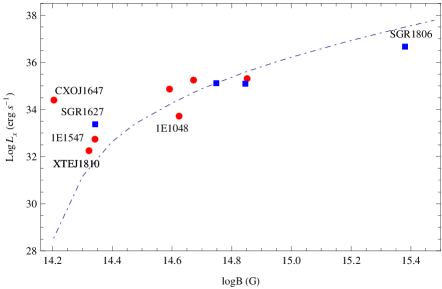
Fig. 2 : The diagram of soft X/$\gamma$-ray luminosity $L_{X}$ as a function of magnetic field strength $B$ when $Y_{e}$= 0.12 and $\rho=\rho_{0}$. Circles and squares are for AXPs and SGRS, respectively. The range of $B$ is assumed to be (1.60 $\times 10^{14}\sim$ 3.0$\times 10^{15}$ G) considering that, when $B\leq B_{f}$, the direct Urca process ceases, while the modified Urca process still occurs, from which weaker X-ray and weaker neutrino flux are produced.

Clearly from Figure 2, the magnetar soft X/$\gamma$-ray luminosity increases with increasing magnetic field obviously, and the steepness of every fitting curve corresponding to weaker magnetic fields ($B<2.5\times 10^{14}$ G) is larger than that corresponding to higher magnetic fields $B\geq 2.5\times 10^{14}$ G), because Eq.(1) is approximately hold only when $B\gg B_{cr}$. For SGR 1806-20 with the lowest value of $\zeta$, whose soft X/$\gamma$ -ray luminosity is cited from (Thompson & Duncan, 1996), its observed value of $L_{X}$ may be biased by the intense low-frequency absorption, corresponding to an electron column density of $\sim$ 6 $\times 10^{22}$ cm^-2 (Murakami et al., 1994; Sonobe et al., 1994), as a result, a significant blackbody component contained in the X-ray bolometric flux is undetected, the luminosity in relativistic particles needed to power the plerion is $\sim$ 5 $\times 10^{36}\times(D/8{\rm kpc})^{2.5}$ erg s^-1 (Thompson & Duncan, 1996). With respect to 1E 1048-59, which is discovered as a 6.4 s dim isolated pulsar near the Carina Nebula (Steward et al., 1986), substantial data were subsequently obtained, showing unambiguous evidence for a large flux increase coupled to a decrease in the pulsed fraction (Mereghetti et al., 2004), as well exemplified by the fact that its $L_{X}$ decreased from (1$\sim$2)$\times 10^{34}$ erg s^-1 (Mereghetti et al., 2004) to 5.4 $\times 10^{33}$ erg s^-1 between September 2004 and April 2011. Therefore, for SGR 1806-20 and 1E1048-59, their values of $\zeta$ are lower than the mean value of $\zeta$ of magnetars, which can be shown in Figure 2. For transient magnetars SGR1627-41, CXOJ1647, 1E11547 .0-5408 and XTEJ1810-197, their observed soft X/$\gamma$-ray luminosities are high than those calculated in theory (far from the fitted curve), the possible explanations are presented as follows:

1. Firstly, with respect to SGR1627-41, its abnormal behavior suggests a connection between the bursting activity and the luminosity of transient magnetars: in 1998 more than 100 bursts in about 6 weeks were observed with different satellites (Woods & Thompson, 2004), however, no other bursts have been reported since then. Its soft X-ray counterpart was identified with BeppoSAX in 1998 at a $L_{X}$ level of $10^{35}$ erg s^-1. Observations carried out in the following 13 years showed a monotonic decrease in its soft X/$\gamma$-ray luminosity, down to the current level of $\sim 2.5\times 10^{33}$ erg s^-1 (to see in Table 4).

2. Second, the first transient AXP XTE J1810-197, discovered in 2003 (Ibrahim et al., 2004), displaced a persistent flux enhancement by a factor of $>$ 100 with respect to quiescent luminosity level $L_{X}$ increased from 7$\times 10^{32}$ erg s^-1 to 5$\times 10^{34}$ erg s^-1 between June 1992 and September 2004 (Bernardini et al., 2009; Gotthelf et al., 2004), however, the latest observations showed an obvious decline in $L_{X}$ (in 10 April 2011 $L_{X}$ $\sim$ 1.9 $\times 10^{32}$ erg s^-1, to see in Table 6). Several other transient magnetars (SGR1627-41,CXOJ1647 and 1E1547.0-5408) have been discovered after XTEJ1810-197. When shining, they have spectral and timing properties analogous with those of the persistent sources. During their ‘quiescent’ phases they universally possess luminosity of $\sim 10^{32}$ erg s ^-1 and soft thermal spectra, that make them similar to CCOs (Mereghetti, 2010). The long-term variations in $L_{X}$ of transient magnetars could be associated with the bursting activities. The source high state coincided with a period of strong bursting activity, while in the following years, during which no bursts were emitted, its luminosity decreased (Mereghetti, 2008).

3. . Finally, the magnetic field strengthes of these four transient magnetars are in the range of $(1.6\sim 2.2)\times 10^{14}$ G, and their values of $L_{X}$ are calculated to be $\sim 10^{28}\sim 10^{31}$ erg s^-1 according to our model. It is not strange that the observed value of $L_{X}$ of a transient magnetar is higher than that calculated if we take into account of the long-term effect of the bursting activity on the soft X/$\gamma$-ray luminosity of a transient magnetar.

What must be emphasised here is that, for AXPs 4U 0142+61 and 1E 2259+586 their mechanisms for persistent soft X/$\gamma$-ray may be related with the accretion, and will be beyond of the scope of our model. The possible explanations are also presented as follows:

1. Firstly, for AXPs 4U 0142+61 and 1E 2259+586 their magnetic field strengthes are lower than the critical magnetic field $B_{f}$. According to our model, once $B\leq B_{f}$, the direct Urca process ceases, while the modified Urca process still occurs, from which weaker X-ray and weaker neutrino flux are produced.

2. Second, the observed properties of 1E 2259+586 seem consistent with the suggestion that it is an isolated pulsar undergoing a combination of spherical and disk accretion (White & Marshall, 1984). This magnetar could be powered by accretion from the remnant of Thorne -$\dot{Z}$ytow object(T$\dot{Z}$) (van Paradijs et al., 1995).

3. Finally, as concerns AXP 4U 0142+61, which was previously considered to be a possible black hole candidate on the basis of its ultra-soft spectrum (White & Marshall, 1984), the simplest explanation for its $L_{X}$ involves a low-mass X-ray binary with a very faint companion, similar to 4U 1627-67(Israel et al., 1994).

Furthermore, timing observations show that the period derivative of SGR 0418+5729, $\dot{P}<$ 6.0 $\times 10^{-15}$ s s^-1, which implies that the corresponding limit on the surface dipolar magnetic field of SGR 0418+5729 is $B<$7.5 $\times 10^{12}$ G (Rea et al., 2010). If the observations are reliable, then the value of $L_{X}$ of SGR 0418+5729 calculated in our model will be far less than $L_{X}\sim(10^{32}-10^{36})$ erg s^-1, which implies that our model is not in contradiction with the observation of SGR 0418+ 5729 (the real value of $L_{X}$ of SGR 0418+5729 is too low to be observed so far). SGR 0418+5729 may present a new challenge to the currently existing magnetar models. However, in accordance with the traditional view on the electron Fermi energy, the electron capture rate $\Gamma$ will decrease with increasing $B$ in ultrastrong magnetic fields. If the electron captures induced by field-decay are an important mechanism powering magnetar’s soft X-ray emission (Cooper & Kaplan, 2010), then $L_{X}$ will also decrease with increasing $B$, which is contrary to the observed data in Table 4 and the fitting result of Figure 2.

4 Conclusions

In this paper, by introducing two important parameters: Landau level-superfluid modified factor and effective X/$\gamma$-ray coefficient, we numerically simulate the process of magnetar cooling and magnetic field decay, and then compute $L_{X}$ of magnetars. We also present a necessary discussion after comparing the observations with the calculations. From the analysis and the calculations above, the main conclusions are as follows:

1. In the interior of a magnetar, superhigh magnetic fields give rise to the increase of the electron Fermi energy, which will induce electron capture reaction.

2. The resulting high-energy neutrons will destroy anisotropic ${}^{3}P_{2}$ neutron Cooper pairs, then the ${}^{3}P_{2}$ anisotropic superfluid and the superhigh magnetic field induced by the ${}^{3}P_{2}$ Cooper pairs will disappear.

3.By colliding, the kinetic energy of the outgoing neutrons will be transformed into thermal energy. This transformed thermal energy would be transported from the star interior to the star surface by conduction, then would be converted into radiation energy as soft X-rays and $\gamma$-rays.

4.The largest advantage of our models is not only to explain but also to calculate magnetar soft X/$\gamma$-ray luminosity $L_{X}$; further, employing the mean value of $\zeta$, we obtain the schematic diagram of $L_{X}$ as a function of $B$. The result of fitting agrees well with the observation result.

Finally, we are hopeful that our assumptions and numerical simulations can be combined with observations in the future, to provide a deeper understanding of the nature of soft X/ $\gamma$-ray of a magnetar.

Acknowledgements We are very grateful to Prof. Qiu-He Peng and Prof. Zi-Gao Dai for their help in improving our presentation. This work is supported by National Basic Research Program of China (973 Program 2009CB824800), Knowledge Innovation Program of The Chinese Academy Sciences KJCX₂ -YW-T09, Xinjiang Natural Science Foundation No.2009211B35, the Key Directional Project of CAS and NSFC under projects 10173020,10673021, 10773005, 10778631 and 10903019.

Appendix

Appendix A The effect of a superhigh magnetic field on $Y_{p}$

In the case of field-free, for reactions $e^{-}+p\rightarrow n+\nu_{e}$ and $n\rightarrow p+e^{-}+\nu^{-}_{e}$ to take place, there exists the following inequality among the Fermi momenta of the proton($p_{F}$), the electron ($k_{F}$)and the neutron ($q_{F}$): $p_{F}+k_{F}\geq q_{F}$ Together with the charge neutrality condition, the above inequality brings about the threshold for proton concentration $Y_{p}\geq$1/9, this means that, in the field-free case, direct Urca reactions are strongly suppressed by Pauli blocking in a system composed of neutrons, protons, and electrons . In the core of a NS, where $\rho\geq 10^{15}$ g cm^-1 and $Y_{p}$ could be higher than 0.11, direct Urca processes could take place (Baiko & Yakovlev, 1999; Lai & Shapiro, 1991; Yakovlev et al., 2001). However, when in a superhigh magnetic field $B\gg B_{cr}$, things could be quite different if we take into account of the effect of the superhigh magnetic field on $Y_{p}$. The effect of a superhigh magnetic field on the NS profiles is gained by applying equations of state (EOS) to solve the Tolman-Oppenheimer-Volkoff equation (Shapiro & Teukolsky, 1983). In the paper of Chakrabarty S. et al (1997), employing a relativistic Hartree theory, authors investigated the gross properties of cold symmetric matter and matter in $\beta-$equilibrium under the influences of ultrastrong magnetic fields. The main conclusions of the paper include: There could be an extremely intense magnetic field $\sim 10^{20}$ G inside a NS; $Y_{p}$ is a strong function of $B$ and $\rho$; when $B$ is near to $B_{cr}^{p}$, the value of $Y_{p}$ is expected to be considerably enhanced, where $B_{cr}^{p}$ is the quantum critical magnetic field of protons ($\sim$1.48 $\times 10^{20}$ G); by strongly modifying the phase spaces of protons and electrons, magnetic fields of such magnitude ($\sim 10^{20}$ G) can cause a substantial $n\rightarrow p$ conversion, as a result, the system is converted to highly proton-rich matter with distinctively softer EOS, compared to the field-free case. Though magnetic fields of such magnitude inside NSs are unauthentic, and are not consistent with our model ($B\sim 10^{14-15}$ G), their calculations are useful in supporting our following assumptions: when $B\sim 10^{14-15}$ G, the value of $Y_{p}$ may be enhanced, and could be higher than the mean value of $Y_{p}$ inside a NS ($\sim$ 0.05); direct Urca reactions are expected to occur inside a magnetar. Based on these assumptions, we can gain a concise expression for $E_{F}(e)$, $E_{F}(e)\simeq$43.44$(\frac{B}{B_{cr}})^{\frac{1}{4}}(\frac{\rho}{\rho_{0}}\frac{Y_{p}}{0.12})^{\frac{1}{4}}$ MeV by solving Eq.(1) of this paper. (Cited from Gao et al.(2011c))

References

- Alpar (2001) Alpar, M. A., 2001, Astrophys. J., 554, 1245
- Baiko & Yakovlev (1999) Baiko D. A., Yakovlev D. G., 1999, Astron. Astrophys., 342, 192-200
- Bernardini et al. (2009) Bernardini, F., Israel, G. L., Dall’Osso, S., 2009, Astron. Astrophys., 498, 195
- Beloborodov & Thompson (2007) Beloborodov, A.M., Thompson, C., 2007, 657, 967
- Canuto & Chiu (1971) Canuto V., Chiu H. Y., 1971, Space Sci. Rev., 12, 3c
- Canuto & Ventura (1977) Canuto V., Ventura J., 1977, Fund. Cosmic Phys., 2, 203
- Chakrabarty et al. (1997) Chakrabarty S., Bandyopadhyay D., Pal S., 1997, Phys. Rev. Lett., 78, 75
- Chatterjee et al. (2000) Chatterjee, P., Hernquist, L., Narayan, R., 2000, Astrophys. J., 534, 373
- Colpi et al. (2000) Colpi, M., Geppert, U., Page, D., 2000, Astrophys. J. Lett., 529, L29
- Cooper & Kaplan (2010) Cooper, R. L., Kaplan, D. L., 2010, Astrophys. J. Lett.,708, L80
- Duncan & Thompson (1992) Duncan R. C., Thompson C., 1992, Astrophys. J., 392, L9
- Duncan & Thompson (1996) Duncan R. C., Thompson C., In: Rothschild R.E., Lingenfelter R.E. (eds.) High-Velocity Neutron Stars and Gamma-Ray Bursts. AIP Conference Proc., vol. 366, p. 111. AIP Press, New York (1996)
- Elgary et al. (1996) Elgary, ., et al., 1996, Phys. Rev. Lett., 77, 1482
- Ertan et al. (2006) Ertan, ., Gş, E., Alpar, M. A., 2006, Astrophys. J., 640, 345
- Ertan & Erkut (2008) Ertan, ., Erkut, M. H., 2008, Astrophys. J., 673, 1062
- Gamov & Schoenberg (1941) Gamov, G., Schoenberg, M., 1941, Phys. Rev, 59, 539
- Gao et al. (2011a) Gao, Z. F., Wang, N., Song, D. L., et al.,2011,Astrophys. Space Sci., DOI:10.1007/s10509-011-0733-7
- Gao et al. (2011b) Gao, Z. F., Wang, N., Yuan, J. P., et al., 2011, Astrophys. Space Sci., 333, 427
- Gao et al. (2011c) Gao, Z. F., Wang, N., Yuan, J. P., et al., 2011, Astrophys. Space Sci.,332, 129
- Ghosh et al. (1997) Ghosh, P., Angelini, L., White, N. E., 1997, Astrophys. J., 478, 713
- Goldreich & Reisenegger (1992) Goldreich, P., Reisenegger, A., 1992, Astrophys. J., 395, 250
- Golenetskii et al. (1984) Golenetskii, S. V., Ilinskii, V. N., Mazets, E. P., 1984, Nature, 307, 41
- Gotthelf et al. (2004) Gotthelf, E.V., Halpern, J. P., Buxton, M., et al., 2004, Astrophys. J., 605, 368
- Halpern et al. (2005) Halpern, J. P., Gotthelf, E. V., Beckek, R. H., et at., 2005, Astrophys. J. Lett., 632, L29
- Harding et al. (1999) Harding, A. K., Contopoulos, I., Kazanas, D., 1999, Astrophys. J. Lett., 525, L125
- Harding & Lai (2006) Harding, A. K., Lai, D., 2006, Rep. Prog. Phys, 69, 2631
- Heyl & Hernquist (1997) Heyl, J. S., Hernquist, L., 1997, Astrophys. J., 489, L67
- Heyl & Kulkarni (1998) Heyl, J. S., Kulkarni, S. R., 1998, Astrophys. J., 506, L61
- Hurley et al. (2005) Hurley, K., Boggs, S. E., Smith, D. M., et al., 2005, Nature, 434, 1098
- Ibrahim et al. (2004) Ibrahim, A. I., Fieire, P. C., Gupta, Y., et al., 2004, Astrophys. J. Lett., 609, L21
- Israel et al. (1994) Israel, G. L., Mereghetti, S., Stella, L., 1994, Astrophys. J., 433, L25
- Kouveliotou et al. (1998) Kouveliotou, C., Dieters, S., Strohmayer, T., et al., 1998, Nature, 393, 235
- Lai & Shapiro (1991) Lai, D., Shapiro, S. L., 1991, Astrophys. J., 383, 745
- Lamb & Pethick et al. (1976) Lamb, D. Q., Pethick, C. J., 1976, Astrophys. J. Lett., 209, L77
- Landau & Lifshitz (1965) Landau, L. D., Lifshitz, E. M., 1965, Quantum mechanics, (Oxford: Pergamon. Press )460
- Langanke & Martinez-Pindo (2000) Langanke, K., Martinez-Pindo, G., 2000, Nucl. Phys. A. 673, 481
- Laros et al. (1986) Laros, J. G., Fenimore, E. E., Fikani, R. W., et al., 1986, Nature, 322, 152
-
Laros et al. (1987)
Laros, J. G., Fenimore, E. E., Klebesadel, M. M., et al.,1987,
Astrophys. J.,320, L111 - Lattimer & Swesty (1991) Lattimer, J. M., & Swesty, F. D. 1991, Nucl. Phys. A, 535, 331
- Leinson & Prez (1997) Leinson, L. B., Prez, A., 1997, arXiv: astro-ph/9711216v2
- Luo et al. (2006) Luo, Z. Q., Liu, M. Q., Peng, Q. H., et al., 2006, Chin. J. Astron. Astrophys., 6, 455
- Lyutikov & Gavrill (2006) Lyutikov, M., Gavriil, F. P., 2006, Mon. Not. R. Astron. Soc., 368, 690
- Marsden et al. (2001) Marsden, D., Lingenfelter, R. E., Rothschild, R. E., et al., 2001, Astrophys. J., 550, 397
- Mazets et al. (1979a) Mazets, E. P., Golenetskij, S. V., Guryan, Y. A., 1979, SvA Lett, 5, 343
- Mazets et al. (1979b) Mazets, E. P., Golenetskij, S. V., Ilinskii, V. N., et al., 1979, Nature, 282, 587
- Mazurek (1976) Mazurek, T. J., 1976, Astrophys. J. Lett., 207, L87
- Mereghetti et al. (2002) Mereghetti, S., Luca, A. D., Caraveo, P. A., et al., 2002, Astrophys. J., 581, 1280
- Mereghetti et al. (2004) Mereghetti, S., Tiengo, A., Stella, L., et al., 2004, Astrophys. J., 608,427
- Mereghetti et al. (2005) Mereghetti, S., Tiengo, A., Esposito, P., et al.,2005,Astrophys. J.,628, 938
- Mereghetti et al. (2006a) Mereghetti, S., Tiengo, A., Turolla, R., et al. 2006,Astron. Astrophys., 450,759
- Mereghetti et al. (2006b) Mereghetti, S., Esposito, P., Tiengo, A., et al.,2006,Astrophys. J.,653, 1423
- Mereghetti (2008) Mereghetti, S., 2008, arXiv: 0804.0250v1[astro-ph]
- Mereghetti (2010) Mereghetti, S., 2010, arXiv: 1008.2891v1[astro-ph.HE]
- Murakami et al. (1994) Murakami, T., Tanaka, Y., Kulkarni, S. R., et al., 1994, Nature, 368, 127
- Nobili et al. (2008) Nobili, L., Turolla, R., Zane, S., 2008, Mon. Not. R. Astron. Soc., 386, 1527
- Peng (2001) Peng, Q. H. 2001, Physics Headway, 21, 225
- Peng & Luo (2006) Peng, Q. H., Luo, Z. Q. 2006, Chin. J. Astron. Astrophys., 6, 248
- Peng & Tong (2007) Peng, Q. H., Tong H., 2007, Mon. Not. R. Astron. Soc., 378, 159
- Peng & Tong (2009) Peng Qiu He., Tong Hao., arXiv: 0911.2066v1 [astro-ph.HE] 11 Nov 2009, Symposium on Nuclei in the Cosmos, 27 July-1 August 2008 Mackinac Island, Michigan,USA
- Pethick (1992) Pethick, C. J., 1992, Rev. Mod. Phys, 6(4), 1133
- Pons et al. (2006) Pons, J. A., Link, B., Miralles, J. A., et al., 2006, arXiv: astro-ph/0607583v3
- Rea et al. (2010) Rea, N., Esposito, P., & Turolla, R., et al., 2010, Science, 330, 944, arXiv: 2010.2781v1
- Rheinhardt & Geppert (2003) Rheinhardt, M., Geppert, U., 2003, Phys. Rev. Lett., 88, 10
- Shapiro & Teukolsky (1983) Shapiro S. L., Teukolsky S. A., 1983, ‘Black holes,white drarfs,and neutron stars’ John Wiley & Sons, New York
- Sonobe et al. (1994) Sonobe, T., Murakami, T., Kulkarni, S. R., et al., 1994, Astrophys. J., 436, L23
- Steward et al. (1986) Steward, F., Charles, P. A., Smale, A. P., 1986, Astrophys. J., 305, 814
- Thompson & Duncan (1993) Thompson, C., Duncan, R. C., 1993, Astrophys. J., 543, 340
- Thompson & Duncan (1995) Thompson, C., Duncan, R. C., 1995, Mon. Not. R. Astron. Soc., 275, 255
- Thompson & Duncan (1996) Thompson, C., Duncan, R. C. 1996, Astrophys. J., 473, 322
- Thompson et al. (2000) Thompson, C., Duncan, R. C., Woods, P. M., 2000, Astrophys. J., 543, 340
- Thompson et al. (2002) Thompson, C., Lyutikov, M., Kulkami, S. R., 2002, Astrophys. J., 574, 332
- Thompson & Beloborodov (2005) Thompson, C., Beloborodov, A.M., 2005,Astrophys. J., 634, 565
- Tong et al. (2009) Tong, H., Xu, R. X., Peng, Q. H., et al., 2009, arXiv: 0906.4223v3[astro-ph.HE]
- Tong et al. (2010) Tong, H., Song, L. M., Xu, R. X., 2010, arXiv: 1009.3620v2 [astro-ph.HE]
- van Paradijs et al. (1995) van Paradijs, J., Taam, R. E., van den Heuvel, E. P. J., 1995, Astron. Astrophys., 299, 41
- Vink & Kuiper (2006) Vink, J., Kuiper, L., 2006, Mon. Not. R. Astron. Soc., 370, L14
- White & Marshall (1984) White, N. E., Marshall, F. E., 1984, Astrophys. J., 281, 354
- Woods & Thompson (2004) Woods, P. M., Thompson, C., 2004,arXiv:astro-ph/0406133
- Yakovlev et al. (2001) Yakovlev, D. G., Kaminker A. D., Gnedin O. Y., et al., 2001, Phys. Rep., 354, 1