Dispersion in Neptune’s Zonal Wind Velocities from NIR Keck AO Observations in July 2009

Abstract

We report observations of Neptune made in H-(1.4-1.8 $\mu$m) and K’-(2.0-2.4 $\mu$m) bands on 14 and 16 July 2009 from the 10-m W.M. Keck II Telescope using the near-infrared camera NIRC2 coupled to the Adaptive Optics (AO) system. We track the positions of 54 bright atmospheric features over a few hours to derive their zonal and latitudinal velocities, and perform radiative transfer modeling to measure the cloud-top pressures of 50 features seen simultaneously in both bands.

We observe one South Polar Feature (SPF) on 14 July and three SPFs on 16 July at $\sim$65^∘S. The SPFs observed on both nights are different features, consistent with the high variability of Neptune’s storms.

There is significant dispersion in Neptune’s zonal wind velocities about the smooth Voyager wind profile fit of Sromovsky et al., Icarus 105, 140 (1993), much greater than the upper limit we expect from vertical wind shear, with the largest dispersion seen at equatorial and southern mid-latitudes. Comparison of feature pressures vs. residuals in zonal velocity from the smooth Voyager wind profile also directly reveals the dominance of mechanisms over vertical wind shear in causing dispersion in the zonal winds.

Vertical wind shear is not the primary cause of the difference in dispersion and deviation in zonal velocities between features tracked in H-band on 14 July and those tracked in K’-band on 16 July. Dispersion in the zonal velocities of features tracked over these short time periods is dominated by one or more mechanisms, other than vertical wind shear, that can cause changes in the dispersion and deviation in the zonal velocities on timescales of hours to days.

Keywords infrared: planetary systems; planets and satellites: Neptune: atmospheres

1 Introduction

The zonal wind velocities of the giant planets can be derived by tracking the motions of cloud features in their atmospheres. Accurate tracking of the motions of cloud features in Neptune’s atmosphere was first achieved with data from the Voyager 2 spacecraft in 1989 (Stone & Miner, 1989). Sromovsky et al. (1993) made a smooth fit to the zonal velocities vs. latitudes of discrete cloud features in Neptune’s atmosphere which were tracked by Limaye & Sromovsky (1991) in Voyager 2 images. Neptune’s canonical zonal wind profile is this smooth Voyager wind profile. The wind velocities derived from individual features in Neptune’s atmosphere since Voyager 2 are observed to remain consistent with this smooth Voyager wind profile, with the exception of features which display significant deviation in zonal velocity, presumably due to mechanisms such as vertical wind shear, wave phenomena, or eddy motions, and which have sometimes been associated with structures such as dark spots (e.g. Hammel & Lockwood 1997; Sromovsky et al. 2001b, c, 2002). Sromovsky et al. (2001c) found deviations from the smooth Voyager wind profile in 1998 HST observations which were consistent with observations in 1995 and 1996 (Sromovsky et al. 2001b), but they concluded that more measurements are needed to confirm a change in Neptune’s zonal wind structure.

Striking dispersion and variation in zonal wind velocities has been observed on Neptune since the Voyager era (Smith et al., 1989). Limaye & Sromovsky (1991) found significant dispersion in zonal wind velocities, with the greatest dispersion found for more short-lived features, and at equatorial and mid-latitudes. Sromovsky et al. (1993) also noted significant deviation in the zonal velocities of cloud features about their smooth Voyager profile fit to the data of Limaye & Sromovsky (1991). Hammel & Lockwood (1997) studied the zonal motions of cloud features in 1995 HST images, along with those for features found in Voyager images (Limaye & Sromovsky 1991; Hammel 1989), Voyager radio occultation data (Lindal et al. 1990), 1991 HST data (Sromovsky et al. 1995), and ground-based data (see Sromovsky et al. (1993) Table VII) and noted that all measurements show dispersion in velocities in narrow bands of latitude, which the authors indicated as evidence for shear, wave phenomena, or other local disturbances. Sromovsky et al. (2001b) found significant deviation in zonal velocities from the smooth Voyager wind profile for features tracked in HST data from 1994, 1995, and 1996. The authors found deviation in 1996 HST data to be mostly associated with a Great Dark Spot at 32^∘N, thought to be the same dark spot seen in 1994 HST images of Neptune at 30^∘N (Hammel et al., 1995). The authors associated dispersion in this region with waves propagating from this Great Dark Spot or associated standing waves.

The more recent analysis of Martin et al. (2012) reveals significant dispersion in zonal wind velocities from the smooth Voyager wind profile. Martin et al. (2012) observed Neptune in H-band with the Keck AO system for 4 hours on UT 20 and 21 August, and for $\sim$1 hour on UT 1 September, 2001. The authors reliably measured the relative velocities of almost 200 clouds in Neptune’s atmosphere, characterizing the dispersion in Neptune’s zonal wind velocities about the smooth Voyager wind profile. The authors found significant dispersion in zonal wind velocity (with variations as high as $\sim$500 m/s), greater than the upper limit they placed on the contribution to dispersion caused by vertical wind shear, and which they attributed primarily to outlying transient clouds that do not move with their local mass flow.

We conduct a similar study as Martin et al. (2012), except we track the motions of Neptune’s cloud features in both H- ($\sim$1.6$\mu$m) and K’- ($\sim$2.2$\mu$m) bands (in observations separated by $\sim$3 Neptune rotations), which are sensitive to a different range of altitudes in Neptune’s atmosphere, to search for potential differences between the two wavelengths. We also perform radiative transfer modeling to estimate the pressures of features. Comparison of the zonal velocities of features with their estimated pressures provides a direct probe of the relative contribution of vertical wind shear to dispersion in the zonal wind velocities. Because our observations in H-band probe a greater overall magnitude and range of depths in Neptune’s atmosphere than those in K’-band, comparing the dispersion observed between the two filters can also give us insight into the relative contribution of vertical wind shear to dispersion in the zonal winds.

In Section 2 we describe our observations and data, including our method of alignment and cylindrical projection of images. In Section 3 we describe our method of tracking the longitude-latitude positions of atmospheric features in our images. Section 4 describes our results for the dispersion in Neptune’s zonal winds, along with our results for the depths of features from radiative transfer modeling, and our observations of the South Polar Features. In Section 5 we discuss our results in the context of a few relevant mechanisms which can cause dispersion in Neptune’s zonal winds and we compare the dispersion observed in H- and K’-bands on 14 and 16 July, respectively. Finally, Section 6 summarizes our conclusions.

2 Data

2.1 Observations and Data Reduction

We observed Neptune from the 10-m W.M. Keck II Telescope on Mauna Kea, Hawaii, on 14 and 16 July 2009 (UT) as part of a project to study the planet’s atmosphere and rings at near-infrared (NIR) wavelengths. H-(1.4-1.8$\mu$m) and K’-(2.0-2.4$\mu$m) band images were taken using the narrow camera of the NIRC2 instrument, coupled to the AO system. The 1024$\times$1024 array has a pixel scale of 9.963$\pm$0.011 mas/pixel in this mode (Pravdo et al., 2006), which at the time of observations corresponded to a physical scale of $\sim$210 km/pixel at disk center.

Although we observed Neptune in both bands on each day, images were more frequently taken in H-band on 14 July and in K’-band on 16 July. On 14 July we took a total of 75 H-band images spanning $\sim$2.5 hours (11:20:21 - 13:47:44 (UT)) and on 16 July we took a total of 105 K’-band images spanning $\sim$3.5 hours (10:54:57 - 14:20:09 (UT)). The integration times of both H- and K’-band images are 60 sec, which provide enough signal to noise without saturating our detector, and assure that smearing due to Neptune’s rotation is less than one image pixel. Short integration times enable a dense sampling of images over time, allowing us to accurately identify the same features in successive images. Our data were taken in $\sim$5-min sequences of five frames each. Largest separations between sequences of images were $\sim$30 min, during which observations of photometric standards were carried out.

We reduced images using standard infrared data reduction techniques of sky subtraction, flat fielding, and median-value masking to remove bad pixels. All images were corrected for the geometric distortion of the array using the ‘dewarp’ routines provided by P. Brian Cameron, who estimates residual errors at $\lesssim$0.1 pixels. We measured angular resolution with the full width at half maxima (FWHM) of Neptune’s moons visible in our images. We measure FWHM in H-band on 14 July of 0.050$\pm$0.004” and in K’-band on 16 July of 0.049$\pm$0.005”, which are consistent with the diffraction limit of our telescope at 2$\mu$m (van Dam et al., 2004), and correspond to effective resolutions of $\sim$1,060 km and $\sim$1,037 km at the center of the disk, respectively.

Images were photometrically calibrated using the star HD201941, and were converted from units of observed flux density to units of I/F, which is defined as (Hammel et al., 1989a):

$$\frac{I}{F}=\frac{r^{2}}{\Omega}\frac{F_{N}}{F_{\odot}},$$ (1)

where $r$ is Neptune’s heliocentric distance, $\pi F_{\odot}$ is the Sun’s flux density at Earth’s orbit (Colina et al., 1996), $F_{N}$ is Neptune’s observed flux density, and $\Omega$ is the solid angle subtended by a pixel on the detector. By this definition, I/F=1 for uniformly diffuse scattering from a Lambert surface when viewed at normal incidence.

2.2 Locations of Cloud Features

Figure 1 shows Neptune images on both days of observation in H-band (left panels) and K’-band (right panels), taken towards the beginning (1st and 3rd rows) and end (2nd and 4th rows) of each night. On both 14 and 16 July we observed Neptune at roughly the same longitudes (these images are separated by $\sim$3 Neptune rotations). We immediately note that atmospheric features tend to be distributed preferentially along bands of constant latitude, with increased prevalence at mid-latitudes, in agreement with previous observations (e.g. Sromovsky et al. 2001b; Max et al. 2003; Irwin et al. 2011; Martin et al. 2012). In addition to clouds at roughly the same latitudes as Martin et al. (2012), we observe clouds at $\sim$40^∘N. In all images there is an absence of cloud features just south of the equator, in agreement with previous observations (e.g. Limaye & Sromovsky 1991; Martin et al. 2012). Atmospheric features vary drastically between 14 and 16 July. Feature morphology changes so dramatically that we cannot with certainty identify the same features present on both nights, as has been noted in previous observations (e.g. Sromovsky et al. 2001b; Karkoschka 2011b).

In all 14 July images we observe a large bright feature centered at $\sim$65^∘S. In 16 July images, centered at the same latitude, we observe three distinct features instead of the large bright feature seen on 14 July. Due to foreshortening effects, these three features appear to begin to coalesce into one as they approach the limb at the end of the night. Features in this latitude region have been identified in previous observations as South Polar Features (SPFs; e.g. Hammel et al. 1989b; Smith et al. 1989; Limaye & Sromovsky 1991; Sromovsky et al. 1993; Crisp et al. 1994; Hammel & Lockwood 1997; Sromovsky et al. 2001b, c; Rages et al. 2002; Karkoschka 2011a; Martin et al. 2012). We will discuss these SPFs in Section 4.4.

In all H-band images we observe a small bright feature at the south pole of the planet. In K’-band we cannot see this feature. This feature has been observed since the Voyager era (e.g. Smith et al. 1989; Limaye & Sromovsky 1991; Hammel et al. 2007; Luszcz-Cook et al. 2010; Karkoschka 2011a). As seen by Limaye & Sromovsky (1991), this feature persisted in the Voyager observations over many Neptune rotations, and the authors were tempted to suggest that it marked the planet’s true rotation pole, as doing so would remove a mean meridional velocity bias which puzzled them. Martin et al. (2012) assumed this ‘south pole dot’ to mark Neptune’s true rotation pole in verifying image navigation, and found the planet center deduced from the south pole dot to agree with that determined from limb fitting within 1 image pixel (16.7$\pm$0.2 mas). There is no a priori reason to assume the feature at the south pole to mark Neptune’s true rotation pole. In fact in previous observations a pair of south polar spots have been seen $\sim$1-2^∘ away from the south pole (Luszcz-Cook et al. 2010; Karkoschka 2011a), and the former authors suggested that these clouds may form in a region of strong convection surrounding a south polar vortex.

2.3 Image Navigation and Cylindrical Projection

To navigate and align our images we must determine the location of the physical center of Neptune in each image to within sub-pixel accuracy. We do so using a multivariate nonlinear $\chi^{2}$ minimization routine which simultaneously fits for the positions of three moons onto their respective orbits for each disk image. The orbit of each moon was derived using the ephemeris generators in the Rings Node of NASA’s Planetary Data System (http://pds-rings.seti.org/). We derive moon orbits rather than use their individual locations given by the ephemeris generators due to uncertainties in the latter (e.g. Jacobsen & Owen 2004; de Pater et al. 2005). This is based on the fitting routine used to align Neptune images by Luszcz-Cook et al. (2010). In 14 July H-band images we fit for the simultaneous positions of Galatea, Larissa, and Despina, and in 16 July K’-band images we fit for the simultaneous positions of Galatea, Larissa, and Proteus. Our mean $\left(x,y\right)$ uncertainties in the derived Neptune centers in our images (calculated from the variance modified by a factor of the reduced-$\chi^{2}$) for H- and K’-bands are (0.08 pix,0.07 pix) and (0.09 pix,0.08 pix), respectively.

The accuracy of the alignment of our images can be judged from Figure 2, which shows mean averages of the stack of aligned images in each filter. The positions of each individual moon trace out visible orbits in the averaged image. In order to better resolve these orbits we high-pass filter each averaged image by subtracting from it an identical image that has been median-smoothed with a width of 30 pixels. High-pass filtering the averaged image eliminates large features that dominate the intensity range and allows high resolution of faint structure such as Neptune’s moons and rings. Neptune’s Adams and Le Verrier rings are clearly visible in both images in Figure 2. In both H- and K’-bands we can clearly distinguish the orbits of Despina, Galatea, and Larissa, although those of Despina and Galatea are difficult to distinguish from the nearby Le Verrier and Adams rings. In K’-band we can also distinguish the orbit of Proteus. We superpose the orbits we derived for these moons in Figure 2. The moon orbits physically traced in our averaged high-pass filtered images align well with the superposed derived moon orbits, reflecting the accuracy of our alignment and Neptune center determinations.

After precise location of Neptune’s center, we transform the data to regularly gridded, cylindrical coordinates, using the same code described in Asay-Davis et al. (2009) and Lii et al. (2010). For the transformation from sky coordinates to planetographic latitude-longitude coordinates on Neptune’s 1-bar surface, we use equations similar to those in Hueso et al. (2010), but simplified with the plane-parallel assumption. Finally, we use IDL’s trigrid function to resample the latitude-longitude data on a regular grid. An example of a transformed image from our cylindrical projection is shown in Figure 3.

3 Tracking Atmospheric Features

We use the velocities of cloud features as a tracer for atmospheric wind velocities, and therefore track the positions of cloud features in our images. After transformation of each image frame, we combine the five frames within each sequence together in a mean average. We track the positions of cloud features in these transformed averaged images. On average, zonal drift rates over 5 min are smaller ($<$0.65^∘/5 min) than an effective angular resolution element at disc center ($\sim$2.4^∘). Averaging images does not significantly smear features and increases signal-to-noise, allowing us to better distinguish faint, fine features. Averaging sets of H-band data from 14 July yields 15 averaged images and averaging sets of K’-band data from 16 July yields 21 averaged images.

In order to track cloud features we first identify them between successive transformed averaged images by constructing images such as Figure 4, which shows successive transformed averaged images in strips of fixed latitude (from 52-30^∘S) stacked with time increasing along the vertical axis.

We define a feature as having an observed brightness distribution distinct from features around it and persisting in at least 4 successive images. Studying Figure 4: bright atmospheric features show a broad range of dynamics. Some features persist relatively consistently in brightness and morphology (blue dashed lines), while others are very ephemeral (yellow dashed lines), appearing and disappearing or significantly varying in morphology on minute timescales. It appears that the smallest features tend also to be the most ephemeral, as was also noted in the Voyager era (Smith et al., 1989). Our initial interpretation of images such as Figure 4 is that features in K’-band evolve more rapidly and appear more ephemeral. This, however, could be due to the greater number of smaller features observed on 16 July. We compare the dispersion in zonal velocities between 14 July H- and 16 July K’-band features in Section 5.2.

After we identify distinct features, we measure their longitude-latitude positions in each transformed averaged image following the method of Martin et al. (2012): for a single feature in a transformed averaged image we take an initial contour of the image at an intensity level that outlines that feature. After isolating this feature we then take three more contours of this feature at intensity levels defined at 60$\%$, 70$\%$, and 80$\%$ of the maximum intensity within the initial contour. We define the center of a feature as the midpoint between longitudinal and latitudinal extrema of a given contour; three individual feature center positions are measured using these three contours. We define the final feature center position as the average of these three measured center positions. The uncertainty in feature center position is defined as the sum in quadrature of the standard deviation of the three measured center positions and navigation uncertainty associated with location of Neptune center position in untransformed images. We repeat this procedure for each tracked feature throughout each of the images in which it is identified. An example illustrating our method is shown in Figure 5.

4 Results

4.1 Deriving Zonal Drift Rates

Our results for 14 July H-band features are shown in Figure 6 and those for 16 July K’-band features are shown in Figure 7. Here we show the longitude positions of each tracked feature versus time, separated into latitude bins identified above each panel.

At fixed latitude, we expect the longitude positions of atmospheric features to move linearly with time, in agreement with the smooth Voyager wind profile of Sromovsky et al. (1993). We expect the latitudinal speeds of most features to be consistent with zero. We derive longitudinal and latitudinal drift rates for each feature by fitting lines to their longitudes vs. time and latitudes vs. time using a Monte-Carlo iteration routine. Our routine fits position vs. time data to a line using the function ladfit in IDL (which fits data to a linear model using a “robust” least absolute deviation method) with each iteration sampling each position measurement from a normal distribution centered on the original position measurement with a width the size of the uncertainty in that measurement. We make $\sim$1,000 iterations until our fits converge. We use the means of the fit parameters from all iterations as our output fit parameters, and the standard deviations of the fit parameters from all iterations as the uncertainties in our output fit parameters.

Our derived drift rates are shown as solid and dotted lines over our data in Figures 6 and 7. Also shown in Figures 6 and 7, overplotted onto each feature using a dashed line, are slopes indicating the longitudinal drift rates expected at the latitude of each feature according to the smooth Voyager wind profile of Sromovsky et al. (1993). We see that, although many features follow constant drift rates, as we expect, there are also many features whose individual longitude positions show significant variation off of these constant drift rates. Non-constant velocities could include true variability, but could also include measurement errors. Sources of error include changes in cloud morphology, image navigation errors, and feature centroiding errors. For instance, anomalous longitude position measurements at $\sim$70 min on July 14 at multiple latitudes argue strongly for some type of measurement error. Therefore, in order to disentangle the effect of large variations in individual longitude position measurements, either real or due to error, from dispersion in derived mean longitudinal drift rates, we separate features by the mean of their absolute residuals in individual longitude position about their derived longitudinal drift rates, $\sigma_{rl}$. Our selection is shown in Figure 8. We divide features into “Low-$\sigma_{rl}$” ($\sigma_{rl}$ $\leq$ 0.7 deg) and “High-$\sigma_{rl}$” ($\sigma_{rl}$ $>$ 0.7 deg). The best-defined feature tracks are in the Low-$\sigma_{rl}$ bin, which contains 25 of 41 July 14 H-band features, and 29 of 46 July 16 K’-band features.

A combination of true variability and unknown sources of uncertainty manifests itself as deviations from linear motion. In order to obtain upper limits to uncertainties for the derived zonal velocities of Low-$\sigma_{rl}$ features, we assume all scatter in the individual measurements of Low-$\sigma_{rl}$ features about their smooth motion is due to unknown errors, and do the following: for each Low-$\sigma_{rl}$ feature whose value for the reduced-$\chi^{2}$ of observed longitude-time data about its derived zonal drift rate is greater than 1, we solve for an additional contribution to the total uncertainty in longitude position such that the reduced-$\chi^{2}$ is equal to 1, assuming this additional source of uncertainty to contribute equally to each longitude position measurement for a given feature, and to be random and uncorrelated with the sources of uncertainty in longitude position already considered; that is, for each Low-$\sigma_{rl}$ feature with $\chi_{red}^{2}>$1 we solve the following expression for an additional unknown source of uncertainty in longitude position, $\sigma_{u}$:

$\chi_{red}^{2}$ = $\frac{1}{N-2}\sum\limits_{i=1}^{N}\frac{\left(\phi_{i}-\phi_{exp,i}\right)^{2}}{\sigma_{cent,i}^{2}+\sigma_{nav,i}^{2}+\sigma_{u}^{2}}$ = 1,

where $N$ is the total number of longitude-time measurements, $\phi_{i}$ are the measured longitude positions, $\phi_{exp,i}$ are the corresponding longitude positions expected from a feature’s derived zonal drift rate, $\sigma_{cent,i}$ is the standard deviation of the three measured feature center positions composing the mean longitude position (from the 60$\%$, 70$\%$, and 80$\%$ intensity contours), and $\sigma_{nav,i}$ is the contribution from navigation uncertainty. Once we solve for $\sigma_{u}$ this way, we include it as a contribution to the uncertainty in each longitude position measurement of its corresponding feature and recompute that feature’s zonal drift rate and its uncertainty in the same way outlined above. The resulting longitude position errors and derived drift rates are those shown in Figures 6 and 7. We make this correction for all Low-$\sigma_{rl}$ features. To quantify the relative magnitude of $\sigma_{u}$, we compute the ratio of $\sigma_{u}$ to the initially estimated sources of longitude position measurement uncertainty ($\eta_{u,i}$ = $\sigma_{u}$/$\left(\sigma_{cent,i}+\sigma_{nav,i}\right)$) for each feature. For 14 July H-band features the mean $\eta_{u}$ is 9.4 and for 16 July K’-band features the mean $\eta_{u}$ is 4.9. We make the same correction for errors in latitude position for all Low-$\sigma_{rl}$ 14 July H-band features and for 25 Low-$\sigma_{rl}$ 16 July K’-band features. Defining a similar $\eta_{u,lat}$ for unknown errors in latitude position: for 14 July H-band features the mean $\eta_{u,lat}$ is 5.9 and for 16 July K’-band features the mean $\eta_{u,lat}$ is 3.4. All uncertainties in feature velocities and drift rates presented here are derived including the contribution of $\sigma_{u}$ to measurement uncertainty. Because $\sigma_{u}$ includes both unknown sources of measurement error and true variability, the uncertainties we present in feature velocities and drift rates are upper limits to the true uncertainties.

We distinguish between High- (red) and Low-$\sigma_{rl}$ (blue) features in Figures 6 and 7. We note that there is a greater number of High-$\sigma_{rl}$ features found in K’-band, probably due to the fact that a greater number of smaller features (which we said tend to be more ephemeral) were observed on 16 July. We note that a number of 16 July K’-band features display a pattern suggestive of east-west temporal oscillation, similar to what was observed by Martin et al. (2012). However, this pattern occurs simultaneously at t$\simeq$50-150 min and with similar periods and phases for a number of features at different locations on the planet. This suggests that the observed pattern may be caused by some type of measurement error, as discussed above. For this reason we also classify these features as High-$\sigma_{rl}$. We focus on Low-$\sigma_{rl}$ features in our analysis of dispersion in wind speeds.

Comparing the drift rates expected from the smooth Voyager wind profile with our derived drift rates in Figures 6 and 7 we note deviation from the smooth Voyager wind profile. Variation in zonal drift rates within individual latitude bins reveals dispersion about the smooth Voyager wind profile. While large deviation from the smooth Voyager wind profile is more frequently found among High-$\sigma_{rl}$ features, for which deviation in drift rate is strongly entangled with scatter in individual position measurement, Low-$\sigma_{rl}$ features show significant dispersion as well. We note, however, that we cannot fully confirm or quantify dispersion in zonal velocities from Figures 6 and 7, because uncertainties in the derived drift rates are not shown. We better quantify the dispersion we observe in Neptune’s zonal wind velocities in what follows.

4.2 Dispersion in Zonal Wind Velocities

We translate the drift rates of atmospheric features into wind velocities according to the following relations:

$$V_{lon}=R_{eq}\cos\theta\frac{d\phi}{dt},$$ (2)

$$V_{lat}=\left(R_{eq}\sin^{2}\theta+R_{pol}\cos^{2}\theta\right)\frac{d\theta}{dt},$$ (3)

where $V_{lon}$ and $V_{lat}$ are the zonal and latitudinal velocities of atmospheric features (m/s), $R_{eq}$=24,766$\times$10³ m is Neptune’s equatorial radius, $R_{pol}$=24,342$\times$10³ m is Neptune’s polar radius, and $d\phi/dt$ and $d\theta/dt$ are derived zonal and latitudinal drift rates (rad/s), where, for $d\phi/dt$, motion from astronomical east to west is taken to be the positive direction. Our derived zonal velocities for 14 July H- and 16 July K’-band Low-$\sigma_{rl}$ features are shown in Figures 9 and 10, respectively, against the smooth Voyager wind profile of Sromovsky et al. (1993) (black solid line). They are also listed for each feature in Tables 2 and 3, along with other relevant quantities associated with the motion of each feature. We plot features such that the size of the square used to represent distinct features increases linearly with the length of time over which a feature was tracked. The longest and shortest tracking times we obtain in H-band are 139 min and 24 min, respectively, and the longest and shortest tracking times we obtain in K’-band are 198 min and 21 min, respectively.

Considering both Figures 9 and 10 we observe significant deviation from and dispersion about the smooth Voyager wind profile. Low-$\sigma_{rl}$ features which scatter most from the smooth Voyager wind profile are those which were tracked for shorter time periods. Increased dispersion is seen at equatorial and southern mid-latitudes. On average, greater dispersion is seen among 14 July H-band features.

Although Low-$\sigma_{rl}$ 16 July K’-band features are on average found to be consistent with the smooth Voyager wind profile within uncertainties, we find significant deviation, $\Delta V_{lon,\sigma}$, for 16 July K’-band features from the smooth Voyager wind profile (including its width of uncertainty) as high as 290$\pm$77 m/s (at the equator). Low-$\sigma_{rl}$ H-band features show a significant average absolute deviation of 177$\pm$55 m/s. Deviation from the smooth Voyager wind profile of 14 July H-band features is found as high as $\sim$500 m/s, although uncertainties in these measurements are large – as high as 25$\%$ at 23^∘S and 50$\%$ at the equator. We more closely examine the difference in dispersion between 14 July H- and 16 July K’-band features in Section 5.2.

Previous studies tracking the motions of Neptune’s cloud features have found significant dispersion and deviation in the zonal velocities. Limaye & Sromovsky (1991) found variation as high as $\sim$750 m/s in the zonal velocities of individual features at fixed latitude, with the greatest variation at equatorial and mid-latitudes. When only considering features whose uncertainties in zonal velocity were $<$25 m/s, the authors found the standard deviation of the zonal velocities about the mean, averaged within 1-degree latitude bins, to be as high as $\sim$275 m/s. Sromovsky et al. (2001b) tracked the motions of bright cloud features in HST data from 1994, 1995, and 1996, and found deviation in zonal velocities from the smooth Voyager profile as high as $\sim$175 m/s for features tracked over time periods ranging from $\sim$1-18 hrs. Martin et al. (2012) found deviation in zonal velocities from the smooth Voyager profile as high as $\sim$500 m/s for features tracked over $\sim$1-4 hrs in NIR Keck AO images of Neptune in 2001. Using the velocities of cloud features as tracers for atmospheric wind velocities, we agree with previous results and observe significant dispersion in Neptune’s wind velocities about its mean zonal wind profile.

4.3 Cloud Feature Pressures From Radiative Transfer Modeling

We use radiative transfer modeling to estimate the pressures of a selection of 50 features that were visible in both H- and K’-bands from the beginning and end of both nights. Model spectra are produced using a 300-layer two-stream radiative transfer code, which is described in detail in Appendix B of Luszcz-Cook (2012). We adopt the temperature profile derived by Fletcher et al. (2010) throughout the atmosphere. We assume a mixing ratio of 0.15 for He and 0.003 for N₂ (Conrath et al., 1993). The methane (CH₄) abundance follows Fletcher et al. (2010) in the upper atmosphere and remains at a mole fraction of 0.022 in the troposphere below the condensation level (Baines et al., 1995). The gas opacity at these wavelengths is dominated by H₂ collision-induced absorption (CIA) and CH₄ opacity; for CIA we use the coefficients for hydrogen, helium and methane from Borysow et al. (1985, 1988) and Borysow (1991, 1992, 1993), assuming an equilibrium ortho/para ratio for H₂. For methane, we use the correlated-k method and follow the recommendations of Sromovsky et al. (2012) for outer planet NIR spectra.

As the spectral information in our data is limited, we use a simplified model of the atmospheric cloud/haze distribution. We assume the presence of an optically thick bottom ‘surface’ cloud and set the depth of this cloud to 2.4 bar. We set the Henyey-Greenstein asymmetry parameter of the bottom cloud to -0.1 (preferentially backscattering) and adjust the single scattering albedo to match the data as described in Luszcz-Cook et al. (2010). Luszcz-Cook (2012) shows that this model fits the $\mu$ dependence of the spectrum in a dark part of Neptune’s disk in field-integral spectroscopic (OSIRIS) data obtained at Keck. For this simplified model, we allow for one additional aerosol layer above the bottom cloud; the particles in this higher-altitude haze/cloud layer are treated as Mie scatterers: we assume that ensembles of particles are distributed according to

$$n\left(r\right)\propto r^{6}\exp\left(-6r/r_{max}\right)$$ (4)

where $n\left(r\right)$ is the number density of particles of radius $r$, and $r_{max}$ is the maximum in the particle distribution (Hansen & Pollack, 1970) and is set to 1.0 $\mu$m (e.g. Irwin et al. 2011). This particle size distribution is analogous to that found on Titan (Mitchell et al., 2011). The extinction cross section and Henyey-Greenstein asymmetry parameter of the scattering are calculated using Mie theory. We assume that the particles have a scale height that is 0.1 times the gas scale height, corresponding to physically thin cloud layers (Irwin et al., 2011). The free parameters in the model are the number density of cloud particles at the bottom (maximum) pressure of the haze/cloud, and the altitude (pressure) of the cloud. For each feature identified in the data for modeling, we fit the observed H- and K’- band I/F values given the viewing geometry ($\mu$) in the following way: for each of 40 model pressure levels distributed (logarithmically) from 3 mbar to 3 bar, we determine the cloud particle number density that would best match the model H-band I/F to the observed H-band I/F. We repeat this procedure for K’-band, then we find the pressure at which the H and K’-band best-fit number densities agree; that is, we determine the pressure at which a cloud of some particle density can best reproduce both the H- and K’-band I/F values.

Cloud-top pressure retrievals are shown in Figures 11$\mathrm{a}$ and 11$\mathrm{b}$. At different latitudes, the range of derived cloud pressures varies by as much as a factor of $\sim$4, with the greatest range in pressures found at southern mid-latitudes (60^∘S to 27^∘S), spanning $\sim$0.5 bar ($\sim$2 scale heights). Clouds at northern latitudes (above 20^∘N) lie at higher altitudes ($\sim$0.1-0.2 bar). We note, however, that clouds at northern latitudes are systematically higher in emission angle, and from these limited data we cannot rule out a systematic bias in the model with $\mu$. Although the 2D relation of pressure vs. $\mu$ in Figure 11$\mathrm{b}$ seems suggestive of a bias with $\mu$, this effect is entangled with any dependence of cloud pressure on latitude, and within fixed latitude bins (including the 3rd dimension shown by symbol shape and color in Figure 11$\mathrm{b}$) there is not an obvious bias with $\mu$. For example, aside from one feature at $\sim$50^∘S found at $\sim$0.6 bar, clouds at equatorial latitudes (27^∘S to 5^∘N) are uniformly found at deeper altitudes ($\sim$0.5 bar) independent of viewing angle.

Our observation that the northern features appear to be at the highest altitudes is consistent with previous authors (e.g. Sromovsky et al. 2001b; Gibbard et al. 2003; Luszcz-Cook 2012). The precise values of the derived northern cloud pressures do not, however, agree with these works, which find them in the stratosphere at 0.023-0.064 bar. We expect these differences to be related to the limitations of our data (we only have broadband measurements, not spectra), differences in the sensitivity of our measurements to different altitudes (for example, Gibbard et al. (2003) measures mostly in K’-band, which is not sensitive to altitudes as deep as those we probe in H-band), and the simplicity of our model – previous studies have favored models with a more complicated haze structure and which vary other model parameters (e.g. Baines & Smith 1990; Gibbard et al. 2002; Irwin et al. 2011; Karkoschka & Tomasko 2011; Luszcz-Cook 2012). Our finding that equatorial features are deepest, while the SPFs in the south are found above them ($\sim$0.3 bar), is different from the results of Gibbard et al. (2003), which suggest a trend of increasing altitude with latitude from south to north. However, clouds at these equatorial latitudes were not observed at the earlier epoch (see Gibbard et al. (2003)).

4.4 South Polar Features

We observe one large bright SPF at 64^∘S on 14 July and three smaller SPFs centered at $\sim$65^∘S on 16 July. SPFs near these latitudes have been seen since the Voyager era (e.g. Smith et al. 1989; Hammel et al. 1989b; Limaye & Sromovsky 1991; Sromovsky et al. 1993, 2001c; Rages et al. 2002; Karkoschka 2011a; Martin et al. 2012) although they have displayed a latitudinal shift, mostly occurring at 67-74^∘S until 2004, and at 60-67^∘S since, consistent with our observations (Karkoschka, 2011a). Individual SPFs are rapidly-evolving features with well-defined periods that cannot be tracked from one planet rotation to the next, and move through the larger structure of the SPF formation region (e.g. Smith et al. 1989; Limaye & Sromovsky 1991; Sromovsky et al. 1993); these features have been observed to form in a fixed longitude region rotating at nearly the planet interior period (Hammel et al., 1989b) – that inferred from Voyager’s radio data tracking Neptune’s magnetic field (Warwick et al. 1989; Lecacheux et al. 1993), then to move East with well-defined periods ranging from 11.7 hr at 74^∘S to 13 hr at 68^∘S, and dissipate before moving halfway around the planet (Limaye & Sromovsky 1991; Sromovsky et al. 1993). At some times, the SPF region can be completely free of bright cloud features (e.g. Sromovsky et al. 1993; Rages et al. 2002). At some times individual SPFs can sporadically form a cloud clump that can be the brightest feature on the disk, with the brightening lasting only tens of hours or less (Rages et al. 2002; Sromovsky et al. 2001c), as we observe on 14 July.

At the beginning of the night on 14 July we observe the large SPF centered at a longitude-latitude position (152^∘W, 64^∘S) to move with a zonal velocity of 272$\pm$15 m/s, consistent with the smooth Voyager wind profile, and a latitudinal speed consistent with zero. At the beginning of the night on 16 July we observe three SPFs at centroid positions (130^∘W, 67^∘S), (119^∘W, 63^∘S), and (92^∘W, 65^∘S) all moving with zonal velocities consistent with the smooth Voyager wind profile except for the SPF at 63^∘S, which moves slower than the smooth Voyager profile by $\Delta V_{lon,\sigma}$=70$\pm$45 m/s. Two 16 July SPFs are found with significant north-south velocities: the SPF at 67^∘S has a northward velocity of 76$\pm$43 m/s, and the SPF at 63^∘S has a southward velocity of 117$\pm$53 m/s. If we extrapolate the zonal drift rate of the 14 July SPF we expect its centroid location at 10:55 on 16 July (UT) to be at a longitude of 40$\pm$14^∘W, whereas the longitudinal extent of the 16 July SPFs does not reach below $\sim$80^∘W at that time. This strongly suggests that the SPFs observed on the two dates are different features, and that storms develop and decay on timescales of hours to days, consistent with previous observations (e.g. Limaye & Sromovsky 1991; Sromovsky et al. 1993, 2001c; Rages et al. 2002).

The dynamics underlying the SPFs have not yet been fully addressed. Sromovsky et al. (1993) found evidence for strong convection driving the SPFs. Karkoschka (2011a) found a rotational lock between the SPF formation region and the South Polar Wave (SPW), a southern n=1 wave spanning the latitudes 65-55^∘S, visible as a dark band in Voyager and HST data (e.g. Smith et al. 1989; Sromovsky et al. 2001a, b). The authors suggested that the vertical motions causing the formation of SPFs are dynamically linked to the SPW, and that the SPW itself is vertically phase-locked with the planet interior. The authors indeed used the motions of the SPF formation region and SPW to infer Neptune’s rotational period (15.9663$\pm$0.0002 hr), different from the 16.11 hr period measured using Voyager’s radio data tracking Neptune’s magnetic field (Warwick et al. 1989; Lecacheux et al. 1993). There is still much to be understood about the dynamics of the SPFs, including their temporal variability.

5 Discussion

Here we briefly discuss a few mechanisms that can cause dispersion in Neptune’s zonal winds which can be addressed by our observations. We then compare the dispersion observed in H-band on 14 July with that observed in K’-band on 16 July.

5.1 Sources of Dispersion

We can constrain the contribution of vertical wind shear to the zonal wind dispersion we observe using our results for the cloud-top pressures of features. We find a range in pressures from $\sim$0.6 bar (at 50^∘S) to $\sim$0.1 bar (northern features), extending approximately 2 scale heights. Voyager IRIS observations of temperature as a function of latitude suggest that at these pressures (30-1000 mbar) Neptune’s vertical wind shear can be on the order of 30 m/s per scale height, with a maximum near the equator (Conrath et al., 1989). For a range in altitudes of 2 scale heights, and assuming that the altitudes of observed cloud features are similar to those for which we derive the cloud-top pressures, vertical wind shear should not contribute more than $\sim$60 m/s to zonal wind dispersion. If we extend this range of depths up to the 2.4 bar bottom cloud we assume in our models and down to 0.02 bar (lower limit for northern features found by Gibbard et al. (2003)), then feature altitudes span no more than $\sim$5 scale heights. For this range of depths vertical wind shear should not contribute more than $\sim$150 m/s to zonal wind dispersion. In many cases we see greater dispersion in zonal wind velocities than what is expected from vertical wind shear, even when considering only Low-$\sigma_{rl}$ features, and especially in H-band. Vertical wind shear cannot be the only cause of the dispersion we observe in the zonal velocities.

We can more directly limit the relative contribution of vertical wind shear to dispersion we observe in the zonal velocities: Figure 11$\mathrm{c}$ shows the cloud-top pressures vs. residuals in zonal velocity from the smooth Voyager wind profile, $\Delta V_{lon}$, of Low-$\sigma_{rl}$ features which were visible in both H- and K’-bands towards the beginning of each night, separated into thin latitude bins extending from 32^∘S to 28^∘N – where, at these altitudes, vertical wind shear is expected to be most important (see Conrath et al. (1989)). Although we do not observe features in any single latitude bin over a wide enough range of pressures to see the vertical wind shear clearly manifest itself given our uncertainties, Figure 11$\mathrm{c}$ directly indicates that one or more other mechanisms dominate over vertical wind shear in producing dispersion in the zonal velocities: there is significant zonal dispersion within latitude bins where features are all estimated to be at about the same pressure (1^∘S to 4^∘N and 26-28^∘N). The zonal dispersion at fixed pressure and at fixed latitudes between 1^∘S and 4^∘N is greater than even the overall upper limit to zonal wind dispersion we expect from vertical wind shear. Features found at 32-29^∘S display the only significant range of pressures ($\sim$0.25-0.45 bar). In this latitude bin we see a spread in zonal velocities significantly greater than what is expected over the range from vertical wind shear ($<$20 m/s), and we do not observe a trend towards higher speed with depth (which at these latitudes is toward more negative velocities), as would be expected from vertical wind shear (see Conrath et al. 1989, 1991).

Along with significant variation in zonal wind velocities at fixed latitude, we also observe some significant north-south feature velocities. Figure 12 shows the derived north-south velocities of Low-$\sigma_{rl}$ features against their latitude positions for both 14 July H- (panel $\mathrm{a}$) and 16 July K’-band (panel $\mathrm{b}$) features. For a few Low-$\sigma_{rl}$ features we find north-south velocities that are convincingly significant, and as high as $\sim$200 m/s. We find that a few features which display significant north-south velocities also display significant deviation in zonal velocities from the smooth Voyager wind profile. Noting significant examples: the 14 July H-band feature at the equator with residual zonal speed $V_{lon,\sigma}$=480$\pm$254 m/s has a southward wind speed 215$\pm$85 m/s. A 14 July H-band feature at 7^∘N is found with residual zonal speed 180$\pm$24 m/s and northward speed 148$\pm$15 m/s. We find a 16 July K’-band feature at 37^∘S with a northward wind speed of 180$\pm$45 m/s and a residual zonal speed of 117$\pm$80 m/s. Again we note the 16 July SPF at 63^∘S with southward velocity 117$\pm$53 m/s and zonal speed residual 70$\pm$45 m/s. Significant north-south velocities and deviations in zonal velocity from the mean zonal profile indicate the presence of one or more mechanisms which can cause both north-south and east-west residual motions. In particular, although we do not confirm the presence of temporal oscillation in our observations, we cannot rule out vortices causing the dispersion we observe. Cloud features centered on or with motions near a vortex would display significant north-south and east-west temporal oscillations, and if these had sufficiently long periods the motions would appear linear on these timescales, with a slope different from the smooth Voyager profile, as we observe. Vortices have often been associated with the dark spots observed on Neptune in Voyager images (such as Voyager GDS and DS2; e.g. Polvani et al. 1990; Sromovsky et al. 1993) and in HST images (such as NGDS-32; e.g. Hammel et al. 1995; Sromovsky et al. 2001b, 2002).

The observed dispersion in zonal velocities and significant north-south velocities imply that we cannot rule out the contribution of wave mechanisms with sufficiently long periods, such as Rossby waves. We do not observe the presence of wave mechanisms which oscillate with periods on the order of our observing period. In particular, we do not observe evidence of tidal forcing by Triton, as was suggested by Martin et al. (2012). Even if we were to assume the motions of those features we noted seemed suggestive of east-west temporal oscillation to be real and not due to error, their periods would not be near the M2 period of tidal forcing by Triton of 7.24 hrs.

From ground-based spectroscopic observations prior to the Voyager encounter, Baines & Smith (1990) found evidence that dynamically driven sublimation and condensation resulting from vertical motions in the atmosphere are responsible for rapid changes observed in Neptune’s clouds. Limaye & Sromovsky (1991) also considered this in the context of the dispersion they observed in the zonal velocities of features in Voyager images. The analysis of Martin et al. (2012) supported this conclusion. The authors noted that if feature velocities represent true fluid velocities, for the fluid to remain nearly divergence-free (for sub-sonic flow), the variation they observed in the zonal velocities with east-west distance ($>$400 m/s over $\sim$20,000 km) would imply large east-west gradients in north-south velocities, which they did not observe, or large vertical motions incompatible with the atmosphere’s gradient Richardson number at the observed altitudes. They therefore confirmed that at least some of the dispersion in zonal velocities they observed is due to transient clouds which do not move with the flow. Our observations also support this result. The spatial distribution of variation in velocities we observe implies that at least some of the dispersion is due to transient clouds, and evidence of cloud motions due to dynamically driven sublimation and condensation is provided by our observations of clouds that are very ephemeral and rapidly change morphology.

5.2 Comparing Dispersion

The results shown in Figures 9 and 10 are immediately suggestive of an overall difference in the magnitude of dispersion in zonal wind velocities about the smooth Voyager wind profile between features tracked in H- and K’-bands on 14 and 16 July, respectively. Whereas 16 July K’-band features seem to agree reasonably well with the smooth Voyager wind profile, 14 July H-band features appear to show overall greater dispersion and deviation from the smooth Voyager profile. The difference in zonal dispersion and deviation between H- and K’-bands might be expected to be a result of the greater range in altitudes probed in H-band over K’-band. Features in H-band can be seen down to larger depths than those in K’-band because the strong absorption of H₂ and CH₄ in K’-band limits detection of features only to higher altitudes (see Luszcz-Cook et al. (2010) Fig. 4). If the difference in zonal velocities is due to the difference in the range of depths probed in H- and K’-bands, then the likely responsible mechanism is vertical wind shear. The effects of vertical wind shear in this difference might be seen in two ways: first, we would expect to see a greater spread in the zonal velocities of features tracked in H-band at fixed latitude; second, and perhaps more subtly, we might expect to see average shifts in the zonal velocities of features between the two bands, consistent with features tracked in H-band on average being at greater depths than those tracked in K’-band. To test the latter of these possibilities we fit Low-$\sigma_{rl}$ $V_{lon}$-$\phi$ data to a polynomial function of the form $V_{lon}$ = $a$ + $b\phi^{2}$ + $c\phi^{4}$ to obtain the best-fit values of $a$, $b$, and $c$ using a Levenberg-Marquardt method, for comparison with the smooth Voyager wind profile fit of Sromovsky et al. (1993). The results of our polynomial fits and the 1$\sigma$ uncertainties (calculated from the variance modified by a factor of the reduced-$\chi^{2}$) are shown with solid and dashed red lines in Figures 9 and 10 and are listed in Table 1, along with the smooth Voyager profile fit of Sromovsky et al. (1993). The zonal velocities of Low-$\sigma_{rl}$ features measured in K’-band on 16 July agree well with the smooth Voyager wind profile (within 1$\sigma$), whereas the zonal velocities of Low-$\sigma_{rl}$ features measured in H-band on 14 July are best represented by a profile which is shifted towards more positive velocities by 180$\pm$50 m/s.

Data	Constant Term (m/s)	$\phi^{2}$ Term (m/s/deg2)	$\phi^{4}$ Term (m/s/deg4)
Voyager	-398$\pm$12	0.188$\pm$0.014	-1.2E-5$\pm$0.3E-5
14 July H-Band	-205$\pm$49	0.083$\pm$0.06	7.0E-6$\pm$14.0E-6
16 July K’-Band	-387$\pm$37	0.165$\pm$0.041	-1.3E-5$\pm$1.1E-5

Table 1 : Polynomial fits to feature zonal velocities vs. latitudes and their 1$\sigma$ uncertainties.

Interestingly, this shift is in the opposite direction from what we would expect due to vertical wind shear. If we assume that most features shown in Figures 9 and 10 are at similar altitudes as those for which we measure the cloud-top pressures, or at least that the zonal direction of the vertical wind shear with pressure is the same at the altitudes of these features as those to which the results of Conrath et al. (1989) and Conrath et al. (1991) apply, then as a result of vertical wind shear we would expect a general decay in zonal speed with height. We observe a shift of our 14 July H-band profile fit towards lower zonal speeds (more positive velocities) at latitudes from $\sim$30^∘S-30^∘N, where the results of Conrath et al. (1989) and Conrath et al. (1991) show the vertical wind shear is most important, and where features that most strongly drive the offset in our profile fit are found. The shift in our profile fit is in the direction we would expect if 14 July H-band features were on average found at higher altitudes than K’-band features. The effects of vertical wind shear are not found in differences in the average zonal velocities of 14 July H- and 16 July K’-band features. We note for clarity that we do not interpret differences in our profile fits to the latitudinal distribution of zonal velocities of Low-$\sigma_{rl}$ features as evidence for a consistent change in Neptune’s mean zonal wind profile from the smooth Voyager wind profile – the short observing times and latitude gaps in our data make it ill-suited to yield evidence for such a claim. In what follows we continue to interpret the smooth Voyager wind profile as describing Neptune’s mean zonal wind profile.

If vertical wind shear were the cause of the apparent difference in zonal dispersion and deviation between 14 July H- and 16 July K’-band features then we would also expect: 1) greater spread in 14 July H-band feature zonal velocities over that of 16 July K’-band feature zonal velocities at fixed latitude; 2) greater deviation from the smooth Voyager wind profile of 14 July H-band feature zonal velocities over that of 16 July K’-band feature zonal velocities at fixed latitude (and this difference in deviation would be fully accounted for by the difference in spread in zonal velocities); 3) differences in the deviation and spread in zonal velocities would not exceed the upper limits we expect for dispersion in the zonal velocities due to vertical wind shear (Section 5.1). To explore this we do the following: we separate $\Delta V_{lon}$ for 14 July H- (squares) and 16 July K’-band (triangles) Low-$\sigma_{rl}$ features (shown in Figure 13$\mathrm{a}$) into latitude bins (shaded bars) chosen according to the latitude bands along which features are observed to be centered (see Figure 1). In each of these latitude bins we compute a weighted average of the absolute value of residuals in zonal velocity of Low-$\sigma_{rl}$ features from the smooth Voyager wind profile, mean $\left|\Delta V_{lon}\right|$, comparing features tracked in H- and K’-bands on 14 and 16 July, respectively (we do not consider uncertainty in the smooth Voyager profile in this calculation, and so these results are useful mainly as a comparison between 14 July H- and 16 July K’-band features). The results are shown in Figure 13$\mathrm{b}$. On average, 14 July H-band features show greater deviation from the smooth Voyager wind profile than K’-band features, and especially at equatorial and southern mid-latitudes.

To directly examine differences in the dispersion in zonal velocity, within each latitude bin where two or more Low-$\sigma_{rl}$ features are found, we compute the difference between the fastest and slowest Low-$\sigma_{rl}$ zonal velocities, max $\delta V_{lon}$ $\equiv$ $\left(\mathrm{max}\,V_{lon}-\mathrm{min}\,V_{lon}\right)$, comparing between 14 July H- and 16 July K’-band features. This is shown in Figure 13$\mathrm{c}$. In many latitude bins uncertainties in the zonal velocities are too large to determine whether or not differences in mean $\left|\Delta V_{lon}\right|$ between 14 July H- and 16 July K’-band features can be fully accounted for by differences in their max $\delta V_{lon}$. Only in the bin of features centered at 30^∘S is there a significant difference in max $\delta V_{lon}$ that can fully account for a corresponding significant difference in mean $\left|\Delta V_{lon}\right|$. However, our comparison in Figure 13 is still useful for making statements about the relative contribution of vertical wind shear to differences in the dispersion in zonal velocities: there are differences in max $\delta V_{lon}$ between Low-$\sigma_{rl}$ 14 July H- and 16 July K’-band features in latitude bins centered at 45^∘S and 23^∘S that are much greater than overall upper limits to dispersion we expect from vertical wind shear. These indicate the dominance of one or more mechanisms other than vertical wind shear causing differences in the dispersion in zonal velocities between 14 July H- and 16 July K’-band features at these latitudes. Maximum possible difference in max $\delta V_{lon}$ in the latitude bin centered at 37^∘S cannot account for the difference in mean $\left|\Delta V_{lon}\right|$ in the same latitude bin; the maximum possible increase in max $\delta V_{lon}$ of these 14 July H-band features over that of 16 July K’-band features (calculated at opposite extremes of their uncertainties) is 172 m/s, whereas 14 July H-band features at these latitudes display mean $\left|\Delta V_{lon}\right|$ greater than that observed for 16 July K’-band features by $>$250 m/s. If we assume that mechanisms which cause deviation in zonal velocities from the smooth Voyager wind profile are similarly capable of causing dispersion in zonal velocities, this also indicates the presence of a mechanism other than vertical wind shear which causes differences in the dispersion in zonal velocities of 14 July H- and 16 July K’-band features.

Our observations indicate the dominance of one or more mechanisms over vertical wind shear in producing the overall dispersion we observe in the zonal winds. That the difference in deviation and dispersion in zonal velocities observed between 14 July H- and 16 July K’-band features is, at least at most latitudes between $\sim$50-20^∘S, not primarily attributable to vertical wind shear further suggests that the mechanisms which dominate dispersion in the zonal winds can cause changes in the magnitude of dispersion and deviation in the zonal winds on timescales of hours to days. This is consistent with the mechanisms discussed above.

6 Summary and Conclusions

In this study we tracked the longitude-latitude positions of Neptune’s atmospheric features seen in Keck AO images in H-band on 14 July 2009 and in K’-band on 16 July 2009 over time. We derived zonal and latitudinal drift rates and velocities for these features. We also performed radiative transfer modeling for features on both nights which were simultaneously visible in both H- and K’-bands. The results we find are the following:

1. We find significant dispersion in the zonal velocities of Neptune’s cloud features about the smooth Voyager wind profile of Sromovsky et al. (1993), with the largest dispersion seen at equatorial and southern mid-latitudes. The observed dispersion is much greater than the upper limit we expect due to vertical wind shear. Considering only Low-$\sigma_{rl}$ features: deviation in zonal velocity from the smooth Voyager wind profile is found as high as 290$\pm$77 m/s (at the equator) among features tracked in K’-band on 16 July, and as high as $\sim$500 m/s among features tracked in H-band on 14 July (although uncertainties for these measurements are as high as 25$\%$ at 23^∘S and 50$\%$ at the equator). Comparison of the zonal velocities and cloud-top pressures of features at fixed latitude also directly indicates the dominance of one or more mechanisms over vertical wind shear in producing dispersion in the zonal winds. Some features display significant north-south velocities (as high as $\sim$200 m/s), and a few of these also display significant deviation in zonal velocity from the smooth Voyager wind profile. This suggests that zonal dispersion is partially due to a mechanism which can produce residual motion along both directions, such as vortices and wave mechanisms with sufficiently long periods so as to appear linear on these timescales, such as Rossby waves. Our observations are consistent with the result that zonal dispersion is caused at least in part by transient clouds due to dynamically driven sublimation and condensation.

2. Radiative transfer modeling indicates that, aside from one feature at 50^∘S found at $\sim$0.6 bar, cloud features at equatorial latitudes ($\sim$5^∘S-5^∘N and 27^∘S-15^∘S) uniformly lie deeper in the atmosphere ($\sim$0.5 bar) while clouds in the north (above 20^∘N) are found at higher altitudes ($\sim$0.1-0.2 bar). Due to limitations of our data, differences in the sensitivity of our measurements to different altitudes, and the simplicity of our model, the precise altitudes we measure for the northern features are different from the results of previous studies, which place them higher, in the stratosphere.

3. We observe one large SPF at 64^∘S on 14 July and three smaller SPFs centered at about the same latitude on 16 July. Two 16 July SPFs display significant north-south velocities, and that with the largest north-south speed (117$\pm$53 m/s southward) also shows significant deviation from the smooth Voyager wind profile (70$\pm$45 m/s slower). Extrapolation of the zonal drift rate of the 14 July SPF and comparison with the average position and spatial extent of the 16 July SPFs shows that the SPFs observed on the two nights are different features, indicating that storms can develop and decay on timescales of hours to days, in agreement with previous observations.

4. There is greater dispersion and deviation observed in the zonal velocities of features tracked in H-band on 14 July than in those tracked in K’-band on 16 July. Polynomial fits to the zonal velocities vs. latitudes of our data show that while 16 July K’-band feature zonal velocities agree well with the smooth Voyager wind profile, 14 July H-band feature zonal velocities are best described by a profile that is shifted toward more positive velocities by 180$\pm$50 m/s. This shift is in the opposite direction from what we would expect if differences in the deviation in zonal velocities from the smooth Voyager wind profile between 14 July H-band and 16 July K’-band features were due to vertical wind shear, as a result of greater average depth of features tracked in H-band. Direct comparison suggests that the difference in deviation and dispersion in zonal velocities between 14 July H- and 16 July K’-band features at fixed latitude is not primarily attributable to vertical wind shear. This further suggests that mechanisms other than vertical wind shear which dominate dispersion in the zonal winds can cause changes in the magnitude of dispersion and deviation in the zonal winds about the mean zonal wind profile on timescales of hours to days.

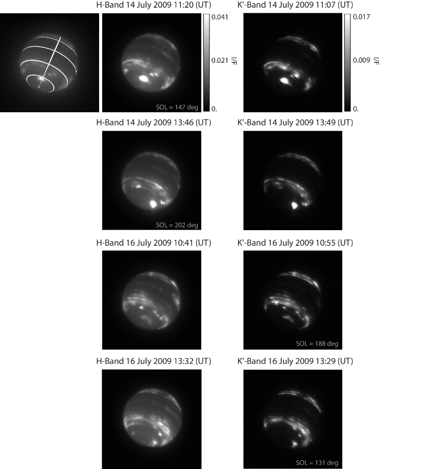
Fig. 1 : Neptune H- (left column) and K’-band (right column) images taken on 14 July 2009 (top two rows) and 16 July 2009 (bottom two rows) towards the beginning (first and third rows) and end (second and fourth rows) of each night. Images are shown in units of I/F according to the scale shown in the colorbars to the right of the topmost images in each filter. For comparison, to the left of the 14 July H-band image taken at 11:20 (UT) (top left panel) we show the same image with overlayed lines of constant latitude (lines are shown at 60^∘S, 30^∘S, the equator, and 30^∘N) and longitude (a line is shown at the sub-observer longitude). The sub-observer longitudes of navigated images are indicated in the bottom right corners of panels.

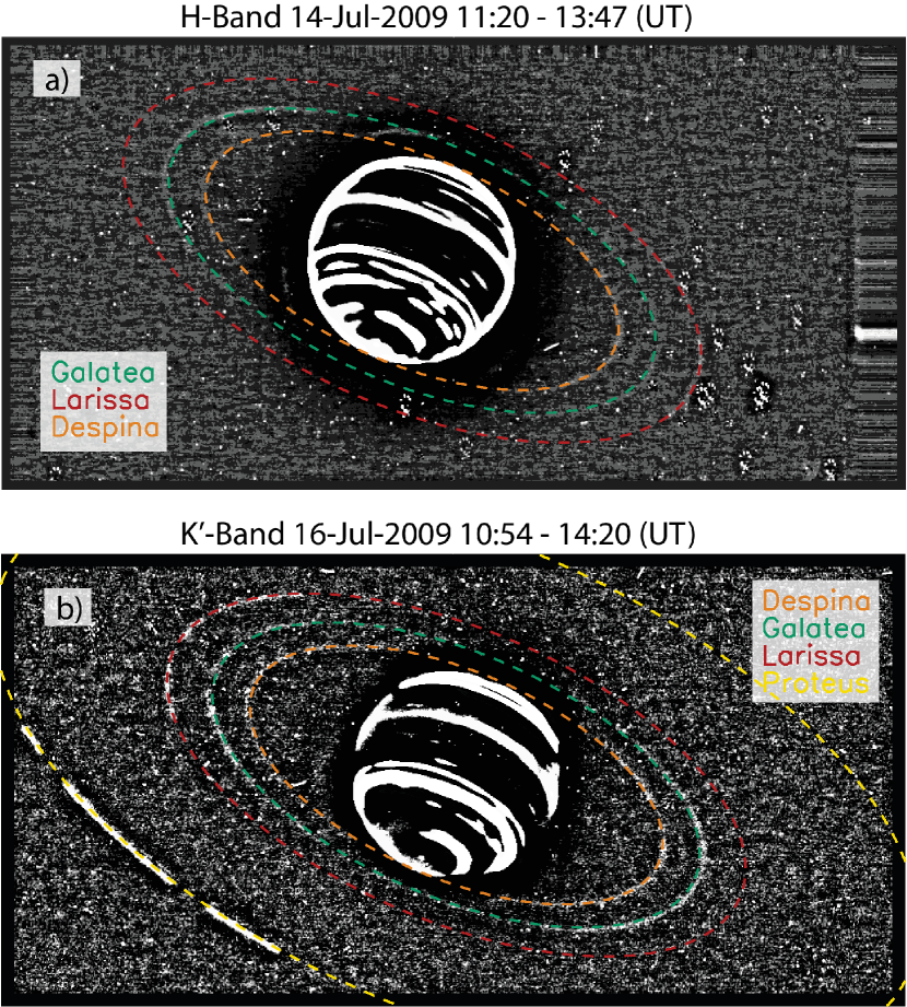
Fig. 2 : Mean averaged, high-pass filtered H- (panel a) and K’-band (panel b) images. H-band image is averaged from the full stack of aligned images from 2009 14 July 11:20:21 - 13:47:44 (UT), and K’-band image is averaged from the stack of aligned images from 2009 16 July 10:54:57 - 14:20:09 (UT). Color dashed lines indicate the derived apparent orbits of Galatea (green), Larissa (red), and Despina (orange) in each image. In K’-band Proteus (yellow) is also indicated. These align well with the true traced moon orbits in each image.

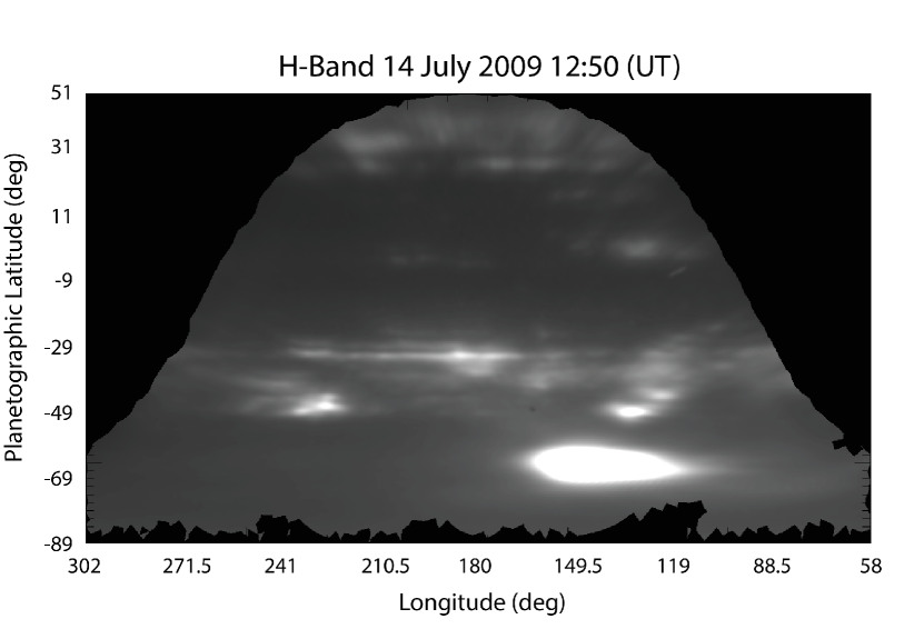
Fig. 3 : Transformed image, taken in H-band on 2009 July 14 12:50:29 (UT).

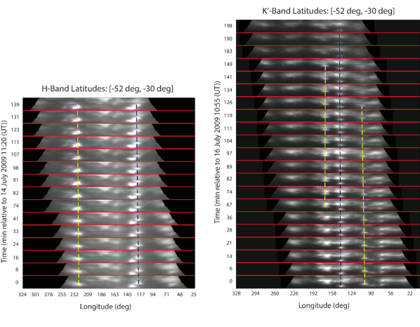
Fig. 4 : Transformed averaged images in strips of fixed latitude (52^∘S-30^∘S) stacked vertically with ascending time. Vertical axis indicates the exposure time of the first of the five images composing the averaged image. Repeating horizontal red lines mark the boundaries between successive image strips. Blue dashed lines indicate representative features which are relatively consistent in brightness and morphology while yellow dashed lines indicate representative features which are more ephemeral and change morphology more significantly and rapidly.

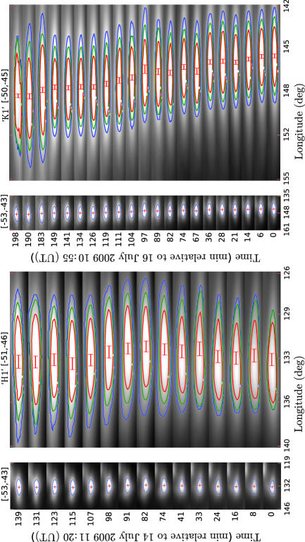
Fig. 5 : Transformed averaged images in strips of fixed latitude – identified at the top of each column – stacked vertically with ascending time. Vertical axis indicates the exposure time of the first of the five images composing the averaged image. Second (fourth) column shows a zoomed-in image of the feature shown in the first (third) column, with contour lines at 60$\%$ (blue), 70$\%$ (green), and 80$\%$ (red) the maximum feature intensity, and our derived feature center indicated to illustrate our feature tracking method. Identifying names are shown above the second and fourth columns in order to easily indicate these features in Figures 6 and 7.

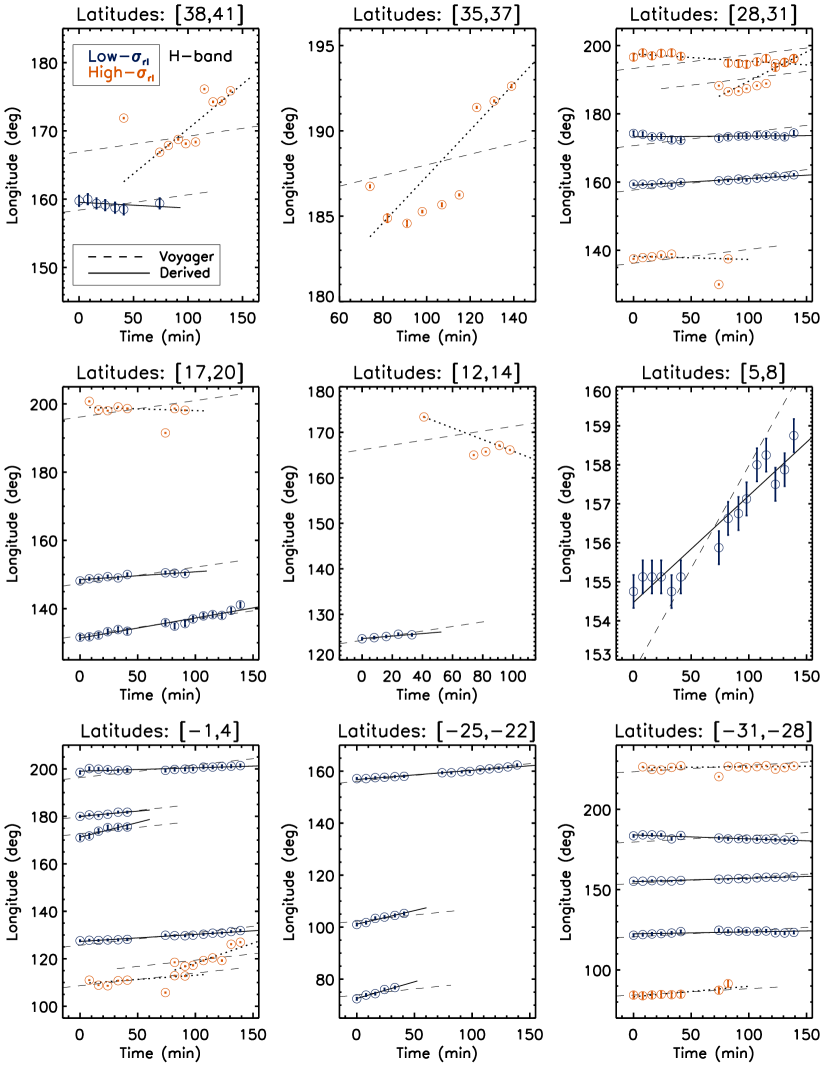
Fig. 6 :

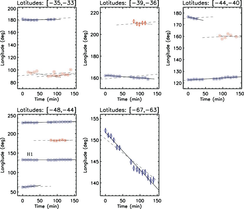
Fig. 6 : Derived zonal drift rates (solid lines and dotted lines) from the longitude positions versus times of each feature tracked in H-band images on 14 July, from 11:20-13:47 (UT), separated into latitude bins indicated at the top of each panel. Time is measured in minutes relative to 2009 July 14 11:20:20 (UT). Zonal drift rates expected at the latitude of each feature according to the smooth Voyager wind profile are shown for comparison (dashed lines). Features are separated by the mean of their absolute residuals in measured longitude position about their derived zonal drift rates: High-$\sigma_{rl}$ (red) and Low-$\sigma_{rl}$ (blue). The feature identified as ‘H1’ in Figure 5 is indicated. Significant dispersion about the smooth Voyager wind profile is observed, even for Low-$\sigma_{rl}$ features.

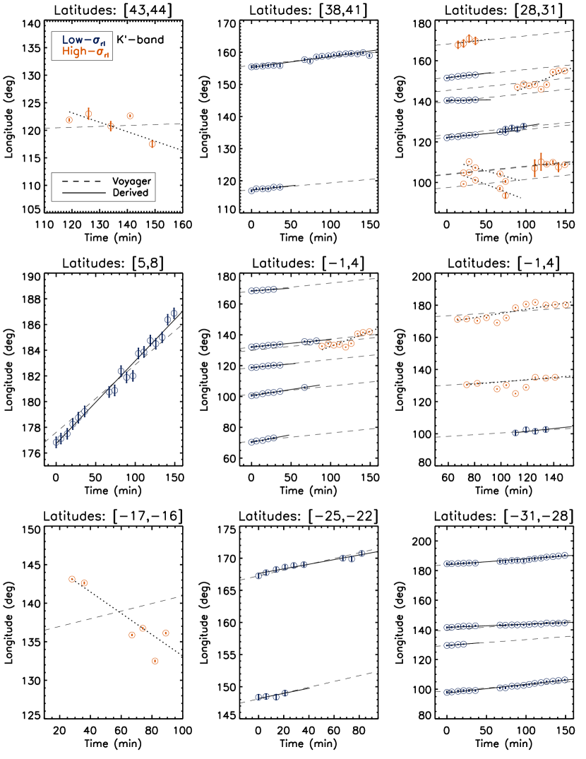
Fig. 7 :

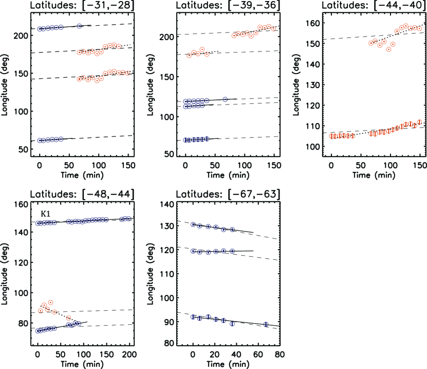
Fig. 7 : Same as Figure 6, now for features tracked in K’-band images on 16 July from 10:54-14:20 (UT). Time is measured in minutes relative to 2009 July 16 10:54:57 (UT). The feature identified as ‘K1’ in Figure 5 is indicated. Significant dispersion about the smooth Voyager wind profile is observed in K’-band on 16 July, even for Low-$\sigma_{rl}$ features.

Fig. 8 : Distribution of the mean of absolute residuals in measured longitude position about the derived zonal drift rates of features, $\sigma_{rl}$. Our two classifications are shown separated by a vertical dashed line: Low-$\sigma_{rl}$ ($\sigma_{rl}$ $\leq$ 0.7 deg) and High-$\sigma_{rl}$ ($\sigma_{rl}$ $>$ 0.7 deg).

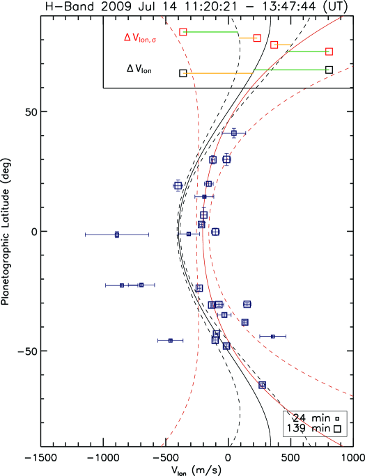
Fig. 9 : Derived zonal velocities of 14 July H-band Low-$\sigma_{rl}$ features shown against the smooth Voyager wind profile (black solid line). The width of uncertainty in the smooth Voyager wind profile is shown with black dashed lines. The length of time over which each feature was tracked is indicated by the size of the square in which each feature’s zonal velocity is plotted. Square sizes corresponding to the shortest and longest tracking times are shown in the bottom left corner. There is significant deviation and dispersion in the zonal velocities from the smooth Voyager wind profile, greater than what is observed on 16 July in K’-band. Our polynomial fit to the zonal velocities vs. latitudes of Low-$\sigma_{rl}$ features is shown with a red solid line, and the widths of uncertainty of our fit are shown with red dashed lines. Our polynomial fit is listed in Table 1 along with the smooth Voyager profile fit of Sromovsky et al. (1993), for comparison. Our polynomial fit to the 14 July H-band feature zonal velocity distribution deviates significantly from the smooth Voyager wind profile, with a shift toward more positive velocities of 180$\pm$50 m/s. A graphical illustration of our two definitions of deviation in the zonal velocities, $\Delta V_{lon,\sigma}$ (red “fake” features) and $\Delta V_{lon}$ (black “fake” features), is shown in the top legend. Green lines illustrate positive values of deviation while yellow lines indicate negative values of deviation, according to the definition of each quantity.

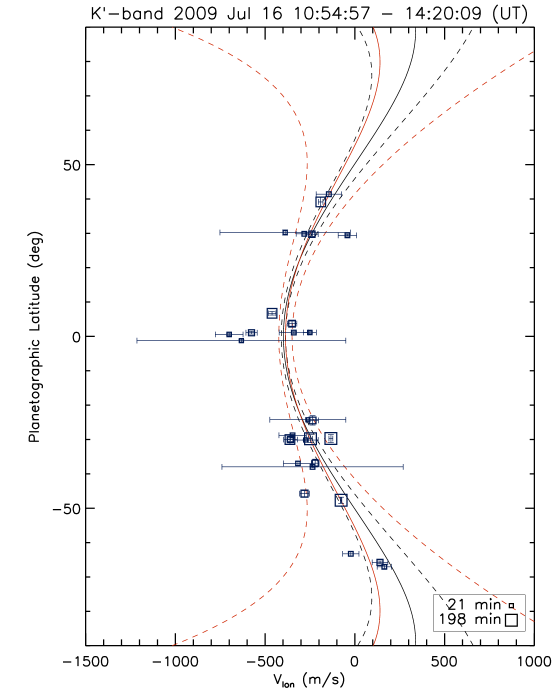
Fig. 10 : Same as Figure 9, now showing the derived zonal speeds of 16 July K’-band Low-$\sigma_{rl}$ features against the smooth Voyager wind profile (black solid line). There is significant deviation and dispersion in zonal velocities from the smooth Voyager wind profile. 16 July K’-band feature zonal velocities agree well (within 1$\sigma$) with the smooth Voyager wind profile in their polynomial fit (red solid line).

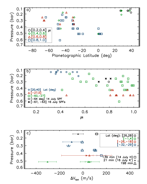
Fig. 11 : a) cloud-top pressures versus latitudes of features seen in both H- and K’-bands on 14 and 16 July. Features are shown in separate bins of the cosine of emission angle, $\mu$, by the color and symbol in which they are plotted, as indicated in the bottom left corner of the panel. b) cloud-top pressures versus $\mu$ of features shown in separate bins of latitude by the color and symbol in which they are plotted, as indicated in the bottom left corner of the panel. Aside from one feature at 50^∘S, equatorial features are uniformly deeper while features in the north are found at higher altitudes. c) the cloud-top pressures vs. residuals in zonal velocity from the smooth Voyager wind profile, $\Delta V_{lon}$, of features for which we were able to make both measurements, from 32^∘S to 28^∘N (where vertical wind shear is expected to be important) in thin bins of latitude. Symbol size indicates the length of time over which a feature was tracked, increasing linearly from the shortest to the longest tracking times indicated in the bottom right corner of the panel. Squares are used to represent features whose velocities were obtained by tracking positions in 14 July H-band images and triangles are used to represent features whose velocities were obtained by tracking positions in 16 July K’-band images.

Fig. 12 : Derived north-south wind speeds $V_{lat}$ versus mean latitude positions of 14 July H- (panel a) and 16 July K’-band (panel b) Low-$\sigma_{rl}$ features. Length of time over which features were tracked is indicated by the size of the symbol in which they are plotted, increasing linearly from the shortest to longest tracking times indicated in each panel.

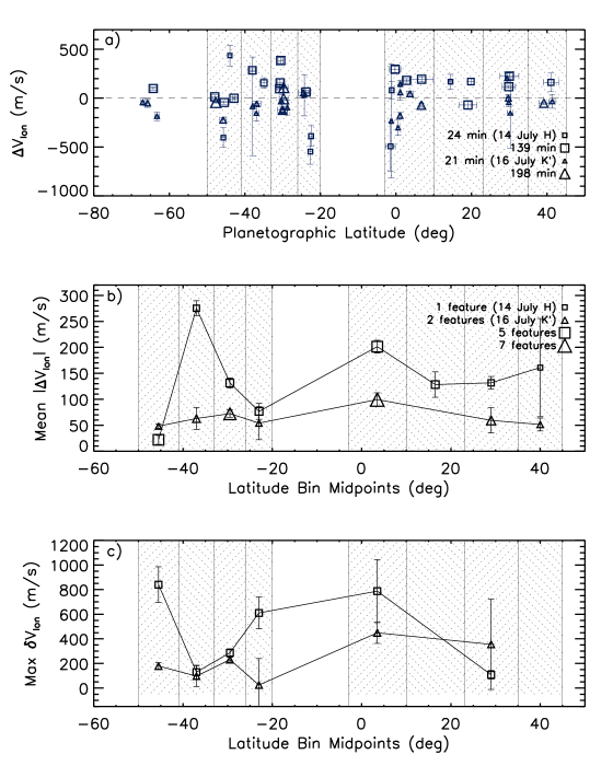
Fig. 13 : a) residuals in zonal velocity from the smooth Voyager wind profile, $\Delta V_{lon}$, for H- (squares) and K’-band (triangles) Low-$\sigma_{rl}$ features. Length of time over which features were tracked is indicated by the symbol size in which each feature is plotted, increasing linearly from the shortest to the longest tracking times in each filter, as indicated in the panel. Latitude bins in which we average the absolute residuals in zonal velocity of features are indicated by shaded bars. b) the mean absolute residuals in zonal velocity from the smooth Voyager wind profile, mean $\left|\Delta V_{lon}\right|$, averaged in the latitude bins indicated, for 14 July H- and 16 July K’-band Low-$\sigma_{rl}$ features. Symbol size indicates the number of features composing the mean average, increasing linearly with the number of features. H-band features on average show greater deviation from the smooth Voyager wind profile. c) Differences between the maximum and minimum zonal velocities of Low-$\sigma_{rl}$ features within each latitude bin (where two or more features are found in each filter), max $\delta V_{lon}$.

Latitude (deg)	$d\phi/dt$ (deg/hr)	$V_{lon}$ (m/s)	$\Delta V_{lon,\sigma}$ (m/s)	$d\theta/dt$ (deg/hr)	$V_{lat}$ (m/s)	$\sigma_{rl}$ (deg)	$\Delta t$ (min)	Nmeas
-64.3$\pm$.7	5.22$\pm$0.28	272$\pm$15	-22$\pm$15	0.09$\pm$0.10	11$\pm$12	0.46	139	15
-48.0$\pm$.9	-0.18$\pm$0.23	-15$\pm$19	-46$\pm$19	0.24$\pm$0.09	28$\pm$10	0.39	139	15
-45.7$\pm$.5	-5.51$\pm$1.20	-462$\pm$101	350$\pm$101	-0.67$\pm$0.57	-79$\pm$68	0.21	33	5
-45.5$\pm$.3	-1.24$\pm$0.20	-105$\pm$17	-10$\pm$17	-0.53$\pm$0.05	-63$\pm$6	0.25	139	15
-44.0$\pm$.6	4.12$\pm$1.21	356$\pm$105	385$\pm$105	-1.30$\pm$0.86	-154$\pm$103	0.16	24	4
-42.9$\pm$.3	-1.07$\pm$0.14	-94$\pm$13	-46$\pm$13	-0.03$\pm$0.04	-4$\pm$5	0.27	139	15
-38.0$\pm$.8	1.41$\pm$0.16	133$\pm$15	246$\pm$15	0.18$\pm$0.12	21$\pm$14	0.25	123	13
-35.0$\pm$.8	-0.32$\pm$0.55	-31$\pm$54	121$\pm$54	-0.55$\pm$0.17	-66$\pm$20	0.38	91	9
-30.8$\pm$.9	-1.29$\pm$0.10	-133$\pm$11	69$\pm$11	-0.31$\pm$0.08	-37$\pm$9	0.17	139	15
-30.6$\pm$.7	-0.73$\pm$0.37	-75$\pm$38	129$\pm$38	0.26$\pm$0.07	31$\pm$8	0.61	139	15
-30.5$\pm$.7	1.46$\pm$0.29	151$\pm$30	357$\pm$30	0.09$\pm$0.10	11$\pm$12	0.36	139	15
-23.8$\pm$.2	-2.11$\pm$0.14	-232$\pm$15	42$\pm$15	-0.47$\pm$0.12	-56$\pm$14	0.19	139	15
-22.7$\pm$.6	-7.69$\pm$1.16	-852$\pm$129	527$\pm$129	-0.79$\pm$0.88	-93$\pm$105	0.20	33	5
-22.5$\pm$.5	-6.26$\pm$0.95	-694$\pm$105	369$\pm$105	0.64$\pm$0.27	75$\pm$32	0.24	41	6
-1.4$\pm$.3	-7.42$\pm$2.12	-891$\pm$254	481$\pm$254	-1.82$\pm$0.72	-215$\pm$85	0.53	41	6
-1.1$\pm$.5	-2.63$\pm$0.72	-316$\pm$87	69$\pm$87	-0.39$\pm$0.43	-46$\pm$51	0.19	41	6
-0.2$\pm$.5	-0.86$\pm$0.26	-103$\pm$31	283$\pm$31	0.40$\pm$0.20	47$\pm$23	0.39	139	15
2.8$\pm$.8	-1.79$\pm$0.14	-215$\pm$17	170$\pm$17	0.28$\pm$0.12	33$\pm$14	0.23	139	15
6.8$\pm$.1	-1.64$\pm$0.20	-196$\pm$24	181$\pm$24	1.26$\pm$0.13	148$\pm$15	0.35	139	15
14.4$\pm$.3	-1.65$\pm$0.65	-191$\pm$76	153$\pm$76	-0.20$\pm$0.40	-23$\pm$47	0.09	33	5
19.1$\pm$.4	-3.54$\pm$0.34	-401$\pm$38	53$\pm$38	-0.11$\pm$0.28	-13$\pm$33	0.50	139	15
19.8$\pm$.9	-1.38$\pm$0.31	-156$\pm$35	152$\pm$35	0.17$\pm$0.26	20$\pm$30	0.25	91	9
29.9$\pm$.8	-1.18$\pm$0.13	-123$\pm$13	90$\pm$13	0.50$\pm$0.21	59$\pm$24	0.19	139	15
30.0$\pm$.5	-0.13$\pm$0.32	-13$\pm$33	198$\pm$33	0.54$\pm$0.33	64$\pm$40	0.42	139	15
41.0$\pm$.1	0.50$\pm$1.04	45$\pm$95	117$\pm$95	-1.17$\pm$1.14	-139$\pm$135	0.38	74	7

Table 2 : Table of various values for Low-$\sigma_{rl}$ features tracked in H-band on 14 July. Definitions of most quantities are given throughout the text. $\Delta t$ is the length of time over which each feature was tracked, and $N_{meas}$ is the number of images in which each feature was measured. For a description of the quantity $\Delta V_{lon,\sigma}$ see footnote 2.

Latitude (deg)	$d\phi/dt$ (deg/hr)	$V_{lon}$ (m/s)	$\Delta V_{lon,\sigma}$ (m/s)	$d\theta/dt$ (deg/hr)	$V_{lat}$ (m/s)	$\sigma_{rl}$ (deg)	$\Delta t$ (min)	Nmeas
-67.0$\pm$.5	3.50$\pm$0.84	164$\pm$39	-95$\pm$39	0.63$\pm$0.36	76$\pm$43	0.17	36	6
-65.7$\pm$.4	2.84$\pm$0.89	140$\pm$44	-78$\pm$44	0.03$\pm$0.31	3$\pm$38	0.34	67	7
-63.3$\pm$.6	-0.42$\pm$0.84	-22$\pm$45	69$\pm$45	-0.98$\pm$0.44	-117$\pm$53	0.16	36	6
-47.7$\pm$.9	-0.95$\pm$0.05	-77$\pm$4	-15$\pm$4	0.08$\pm$0.04	9$\pm$5	0.15	198	21
-45.8$\pm$.9	-3.35$\pm$0.32	-281$\pm$27	169$\pm$27	-0.61$\pm$0.05	-72$\pm$6	0.21	89	10
-38.0$\pm$.2	-2.49$\pm$5.34	-235$\pm$505	45$\pm$505	0.26$\pm$0.42	31$\pm$50	0.14	36	6
-37.0$\pm$.6	-3.31$\pm$0.84	-317$\pm$81	117$\pm$81	1.52$\pm$0.37	181$\pm$44	0.15	28	5
-36.9$\pm$.1	-2.30$\pm$0.23	-221$\pm$22	20$\pm$22	1.07$\pm$0.11	127$\pm$13	0.09	67	7
-30.2$\pm$.1	-2.64$\pm$0.67	-274$\pm$70	10$\pm$70	0.20$\pm$0.59	24$\pm$70	0.05	21	4
-30.0$\pm$.4	-3.48$\pm$0.16	-361$\pm$17	96$\pm$17	-0.1$\pm$0.15	-12$\pm$18	0.32	149	18
-30.0$\pm$.5	-3.45$\pm$0.37	-359$\pm$38	93$\pm$38	0.42$\pm$0.15	50$\pm$18	0.16	67	7
-29.8$\pm$.2	-2.37$\pm$0.11	-247$\pm$11	-20$\pm$11	0.15$\pm$0.07	17$\pm$9	0.37	198	21
-29.7$\pm$.1	-1.28$\pm$0.10	-133$\pm$11	81$\pm$11	0.32$\pm$0.05	39$\pm$6	0.25	198	21
-28.8$\pm$.1	-3.30$\pm$0.73	-347$\pm$76	71$\pm$76	-0.1$\pm$0.14	-12$\pm$17	0.15	36	6
-24.4$\pm$.4	-2.15$\pm$0.29	-235$\pm$32	33$\pm$32	-0.86$\pm$0.24	-101$\pm$29	0.20	82	9
-24.2$\pm$.1	-2.39$\pm$1.94	-262$\pm$212	8$\pm$212	0.02$\pm$0.15	2$\pm$17	0.16	21	4
-1.2$\pm$.4	-5.27$\pm$4.85	-632$\pm$582	223$\pm$582	0.95$\pm$0.28	112$\pm$33	0.47	23	4
0.6$\pm$.4	-5.83$\pm$0.64	-700$\pm$77	290$\pm$77	-0.60$\pm$0.52	-70$\pm$62	0.12	28	5
1.1$\pm$.4	-4.80$\pm$0.26	-576$\pm$31	166$\pm$31	-0.17$\pm$0.17	-20$\pm$20	0.12	67	7
1.1$\pm$.3	-2.83$\pm$0.68	-340$\pm$82	46$\pm$82	0.07$\pm$0.42	8$\pm$50	0.13	36	6
1.1$\pm$.2	-2.09$\pm$0.30	-251$\pm$37	135$\pm$37	0.10$\pm$0.62	12$\pm$73	0.05	28	5
3.7$\pm$.8	-2.92$\pm$0.22	-350$\pm$26	33$\pm$26	0.48$\pm$0.12	56$\pm$14	0.14	82	9
6.7$\pm$.5	-3.87$\pm$0.17	-461$\pm$21	59$\pm$21	0.12$\pm$0.06	14$\pm$7	0.34	149	18
29.4$\pm$.2	-0.40$\pm$0.49	-41$\pm$51	177$\pm$51	0.32$\pm$0.28	38$\pm$33	0.11	36	6
29.7$\pm$.6	-2.30$\pm$0.34	-240$\pm$35	-25$\pm$35	0.49$\pm$0.09	58$\pm$11	0.15	74	8
29.9$\pm$.1	-2.70$\pm$0.44	-282$\pm$45	15$\pm$45	0.01$\pm$0.21	1$\pm$25	0.09	36	6
30.2$\pm$.8	-3.74$\pm$3.50	-388$\pm$363	125$\pm$363	0.51$\pm$2.48	61$\pm$294	0.33	23	4
39.1$\pm$.40	-2.04$\pm$0.13	-190$\pm$13	12$\pm$13	0.05$\pm$0.15	6$\pm$17	0.33	149	18
41.4$\pm$.7	-1.61$\pm$0.78	-145$\pm$70	-11$\pm$70	-0.05$\pm$1.03	-6$\pm$123	0.14	36	6

Table 3 : Table of various values for Low-$\sigma_{rl}$ features tracked in K’-band on 16 July. Definitions of most quantities are given throughout the text. $\Delta t$ is the length of time over which each feature was tracked, and $N_{meas}$ is the number of images in which each feature was measured. For a description of the quantity $\Delta V_{lon,\sigma}$ see footnote 2.

References

- Allison & Lumetta (1990) Allison, M., Ferguson, J.W.: Geophys. Res. Lett. 17, 2269 (1990)
- Asay-Davis et al. (2009) Asay-Davis, X.S., Marcus, P.S., Wong, M.H., de Pater, I.: Icarus 203, 164 (2009)
- Baines & Smith (1990) Baines, K.H., Smith, H.Wm.: Icarus 85, 65 (1990)
- Baines et al. (1995) Baines, K.H., Mickelson, M.E., Larson, L.E., Ferguson, D.W.: Icarus 114, 328 (1995)
- Borysow et al. (1985) Borysow, J., Trafton, L., Frommhold, L., Birnbaum, G.: Astrophys. J. 296, 644 (1985)
- Borysow et al. (1988) Borysow, J., Frommhold, L., Birnbaum, G.: Astrophys. J. 326, 509 (1988)
- Borysow (1991) Borysow, A.: Icarus 92, 273 (1991)
- Borysow (1992) Borysow, A.: Icarus 96, 169 (1992)
- Borysow (1993) Borysow, A.: Icarus 106, 614 (1993)
- Colina et al. (1996) Colina, L., Bohlin, R.C., Castelli, F.: Astron. J. 112, 307 (1996)
- Conrath et al. (1989) Conrath, B., Flasar, F.M., Hanel, R., Kunde, V., Maguire, W., Pearl, J., Pirraglia, J., Samuelson, R., Cruikshank, D., Horn, L.: Science 246, 1454 (1989)
- Conrath et al. (1991) Conrath, B.J., Flasar, F.M., Gierasch, P.J.: J. Geophys. Res. 96, 18931 (1991)
- Conrath et al. (1993) Conrath, B.J., Gautier, D., Owen, T.C., Samuelson, R.E.: Icarus 101, 168 (1993)
- Crisp et al. (1994) Crisp, D., Trauger, J., Stapelfeldt, K., Brooke, T., Clarke, J., Ballester, G., Evans, R., WFPC2 Science Team: Bull. Am. Astron. Soc. 26, 1093 (1994)
- de Pater et al. (2005) de Pater, I., Gibbard, S.G., Chiang, E., Hammel, H.B., Macintosh, B., Marchis, F., Martin, S.C., Roe, H.G., Showalter, M.: Icarus 174, 263 (2005)
- Fletcher et al. (2010) Fletcher, L.N., Drossart, P., Burgdorf, M., Orton, G.S., Encrenaz, T.: Astron. Astrophys. 514, A17 (2010)
- Gibbard et al. (2002) Gibbard, S.G., Roe, H., de Pater, I., Macintosh, B., Gavel, D., Max, C.E., Baines, K.H., Ghez, A.: Icarus 156, 1 (2002)
- Gibbard et al. (2003) Gibbard, S.G., de Pater, I., Roe, H.G., Martin, S., Macintosh, B.A., Max, C.E.: Icarus 166, 359 (2003)
- Hammel (1989) Hammel, H.B.: Icarus 80, 14 (1989)
- Hammel et al. (1989a) Hammel, H.B., Baines, K.H., Bergstrahl, J.T.: Icarus 80, 416 (1989a)
- Hammel et al. (1989b) Hammel, H.B., Beebe, R.F., de Jong, E.M., Hansen, C.J., Howell, C.D., Ingersoll, A.P., Johnson, T.V., Limaye, S.S., Magalhaes, J.A., Pollack, J.B., Sromovsky, L.A., Suomi, V.E., Swift, C.E.: Science 245, 1367 (1989b)
- Hammel et al. (1995) Hammel, H.B., Lockwood, G.J., Mills, J.R., Barnet, C.D.: Science 268, 1740 (1995)
- Hammel & Lockwood (1997) Hammel, H.B., Lockwood, G.W.: Icarus 129, 466 (1997)
- Hammel et al. (2007) Hammel, H.B., Sitko, M.L., Lynch, D.K., Orton, G.S., Russell, R.W., Geballe, T.R., de Pater, I.: Astron. J. 134, 637 (2007)
- Hansen & Pollack (1970) Hansen, J.E., Pollack, J.B.: J. Atmos. Sci. 27, 265 (1970)
- Hueso et al. (2010) Hueso, R., Legarreta, J., Rojas, J.F., Peralta, J., Pérez-Hoyos, S., del Río-Gaztelurrutia, T., Sánchez-Lavega, A.: Adv. Spac. Res. 46, 1120 (2010)
- Irwin et al. (2011) Irwin, P.G.J., Teanby, N.A., Davis, G.R., Fletcher, L.N., Orton, G.S., Tice, D., Hurley, J., Calcutt, S.B.: Icarus 216, 141 (2011)
- Jacobsen & Owen (2004) Jacobsen, R.A., Owen, Jr., W.M.: Astron. J. 128, 1412 (2004)
- Karkoschka & Tomasko (2011) Karkoschka, E., Tomasko, M.G.: Icarus 211, 780 (2011)
- Karkoschka (2011b) Karkoschka, E.: Icarus 215, 759 (2011b)
- Karkoschka (2011a) Karkoschka, E.: Icarus 215, 439 (2011a)
- Lecacheux et al. (1993) Lecacheux, A.,Zarka, Ph.,Desch, M.D.,Evans, D.R.: Geophys. Res. Lett. 20, 2711 (1993)
- Lii et al. (2010) Lii, P.S., Wong, M.H., de Pater, I.: Icarus 209, 591 (2010)
- Limaye & Sromovsky (1991) Limaye, S.S., Sromovsky, L.A.: J. Geophys. Res. 96, 18941 (1991)
- Lindal et al. (1990) Lindal, G.F., Lyons, J.R., Sweetnam, D.N., Eshleman, V.R., Hinson, D.P., Tyler, G.L.: Bull. Am. Astron. Soc. 22, 1106 (1990)
- Luszcz-Cook et al. (2010) Luszcz-Cook, S.H., de Pater, I., Ádámkovics, M., Hammel, H.B.: Icarus 208, 938 (2010)
- Luszcz-Cook (2012) Luszcz-Cook, S. 2012, “Millimeter and Near-Infrared Observations of Neptune’s Atmospheric Dynamics”, PhD Thesis, University of California, Berkeley
- Martin et al. (2012) Martin, S.C., de Pater, I., Marcus, P.: Astrophys. Space Sci. 337, 65 (2012)
- Max et al. (2003) Max, C.E., Macintosh, B.A., Gibbard, S.G., Gavel, D.T., Roe, H.G., de Pater, I., Ghez, A.M., Acton, D.S., Lai, O., Stomski, P., Wizinowich, P.L.: Astron. J. 125, 364 (2003)
- Mitchell et al. (2011) Mitchell, J.L., Ádámkovics, M., Caballero, R., Turtle, E.P.: Nat. Geo. 4, 589 (2011)
- Polvani et al. (1990) Polvani, L.M., Wisdom, J., Dejong, E., Ingersoll, A.P.: Science 249, 1393 (1990)
- Pravdo et al. (2006) Pravdo, S.H., Shaklan, S.B., Wiktorowicz, S.J., Kulkarni, S., Lloyd, J.P., Martinache, F., Tuthill, P.G., Ireland, M.J.: Astrophys. J. 649, 389 (2006)
- Rages et al. (2002) Rages, K., Hammel, H.B., Lockwood, G.W.: Icarus 159, 262 (2002)
- Smith et al. (1989) Smith, B.A., et al.: Science 246, 1422 (1989)
- Sromovsky et al. (1993) Sromovsky, L.A., Limaye, S.S., Fry, P.M.: Icarus 105, 140 (1993)
- Sromovsky et al. (1995) Sromovsky, L.A., Limaye, S.S., Fry, P.M.: Icarus 118, 25 (1995)
- Sromovsky et al. (2001a) Sromovsky, L.A., Fry, P.M., Baines, K.H., Dowling, T.E.: Icarus 149, 435 (2001a)
- Sromovsky et al. (2001b) Sromovsky, L.A., Fry, P.M., Dowling, T.E., Baines, K.H., Limaye, S.S.: Icarus 149, 459 (2001b)
- Sromovsky et al. (2001c) Sromovsky, L.A., Fry, P.M., Dowling, T.E., Baines, K.H., Limaye, S.S.: Icarus 150, 244 (2001c)
- Sromovsky et al. (2002) Sromovsky, L.A., Fry, P.M., Baines, K.H.: Icarus 156, 16 (2002)
- Sromovsky et al. (2012) Sromovsky, L.A., Fry, P.M., Boudon, V., Campargue, A., Nikitin, A.: Icarus 218, 1 (2012)
- Stone & Miner (1989) Stone, E.C., Miner, E.D.: Science 246, 1417 (1989)
- van Dam et al. (2004) van Dam, M.A., Le Mignant, D., Macintosh, B.A.: Proc. SPIE 5490, 174 (2004)
- Warwick et al. (1989) Warwick, J.W., et al.: Science 246, 1498 (1989)