Comparative quantum and semi-classical analysis of Atom-Field Systems II: chaos and regularity

Abstract

The non-integrable Dicke model and its integrable approximation, the Tavis-Cummings (TC) model, are studied as functions of both the coupling constant and the excitation energy. The present contribution extends the analysis presented in the previous paper by focusing on the statistical properties of the quantum fluctuations in the energy spectrum and their relation with the excited state quantum phase transitions (ESQPT). These properties are compared with the dynamics observed in the semi-classical versions of the models. The presence of chaos for different energies and coupling constants is exhibited, employing Poincaré sections and Peres lattices in the classical and quantum versions, respectively. A clear correspondence between the classical and quantum result is found for systems containing between $\mathcal{N}=80$ to $200$ atoms. A measure of the Wigner character of the energy spectrum for different couplings and energy intervals is also presented employing the statistical Anderson-Darling test. It is found that in the Dicke Model, for any coupling, a low energy regime with regular states is always present. The richness of the onset of chaos is discussed both for finite quantum systems and for the semi-classical limit, which is exact when the number of atoms in the system tends to infinite.

I Introduction

The Dicke and Tavis-Cummings (TC) Hamiltonian describe a system of $\mathcal{N}$ two-level atoms interacting with a single monochromatic electromagnetic radiation mode within a cavity Dicke54 . One of the most representative feature of these Hamiltonians is their second-order quantum phase transition (QPT) in the thermodynamic limit Hepp73 ; Wang73 (equivalent in the present models to the semi-classical limit). The ground state of the system goes from a normal to a superradiant state when the atom-field interaction reaches a critical value. In a companion paper Basta1 , hereon referred to as (I), it was shown that the semi-classical approximation to the density of states (DoS) describes very well the averaged quantum density of states (QDoS). From the semi-classical description, the presence of two different excited-state quantum phase transitions (ESQPTs) was clearly established in these models. One ESQPT, referred to as static, occurs for any coupling at an energy $E/(\omega_{o}j)=1$, where the whole phase space associated with the two-levels atoms (the pseudo-spin sphere) becomes available for the system. The second ESQPT, referred to as dynamic, can take place only in the superradiant phase, at energies $E/(\omega_{o}j)=-1$. This transition occurs when the top of the double well (Dicke) or mexican hat (TC) potential that develops in the superradiant phase is attained.

The previous results allow to study the properties of the quantum fluctuations using the semi-classical DoS to separate the tendency or secular variation of the spectrum from its fluctuations. It is known that the tendency of the QDoS depends completely on the particular system, but the properties of the fluctuations are universal Haake . For quantum systems with a classical analogue integrable the fluctuations are common with those of the so-called Gaussian Diagonal Ensemble (GDE), while for time-reversal-symmetric quantum systems with classical analogue hard chaotic, the fluctuations are those of the Gaussian Orthogonal Ensemble (GOE).

In Ref. Emary03 numerical evidence was presented that suggests a relationship between the normal to superradiant phase transition and the onset of chaos in the non-integrable Dicke model. More recently Per11A this relationship was studied more closely and it was suggested that the onset of chaos is caused by the precursors of the dynamic ESQPT occurring in the superradiant phase. In this contribution we go further in the study of this relationship between the onset of chaos and singular behavior of the DoS (ESQPT) and ground-state energy (QPT). To this end we consider the non-integrable Dicke model and its integrable approximation, the Tavis-Cummings model. We study these models as a function of both the coupling between atoms and field, and the excitation energy. The presence of chaos for different energies and coupling constants is exhibited, in the semi-classical limit, employing Poincaré sections. The role of the classical chaos in the Dicke model has been recently studied in the context of the equilibration of unitary quantum dynamics Alt12 . In the quantum case Peres lattices are presented, which allow to characterize regular and chaotic regions qualitatively. A quantitative measure of the properties of the energy spectrum is also presented by means of testing if the Nearest Neighbor Spacing Distribution (NNSD) of the unfolded energies follows the Wigner distribution of the GOE. The results of the classical model are compared to the quantum ones. Similar to the results of Ref.Bakemeier13 , a clear correspondence between classical and quantum results are found for finite quantum system ranging from $\mathcal{N}\sim 80$ to $\mathcal{N}\sim 200$.

It is found that the onset of chaos in the Dicke model can only take place in the energy region where the quadratic approximation of the Hamiltonian, the one obtained by considering small oscillations around the global energy minimum, fails to describe semiclassical model dynamics.For any coupling there always exist a low energy interval above the ground state where only regular patterns are observed. In particular, for the very small coupling regime $\gamma\approx 0$ this energy interval extends to infinity. Above these low energy region the quadratic approximation breaks down and room is left for the onset of chaos. Even if an indirect connection between the ESQPTs and the onset of chaos can be identified through the unstable fixed points, the onset of chaos is a much richer phenomenon than the occurrence of non-analytic behavior in the density of states or the ground-state energy.

The article is organized as follows: in Section II we present briefly the Quantum Dicke and Tavis-Cummings Hamiltonians and their classical analogues, and summarize some of their properties. In section III a qualitatively analysis of the spectrum is done via Peres lattices and Poincaré sections, revealing a clear classical and quantum correspondence at the onset of chaos, both in the normal and superradiant phases. The properties of the energy fluctuations are studied by means of the Anderson-Darling test for the NNSD against the Wigner distribution. Section IV contains the conclusions.

II Dicke and Tavis-Cummings Hamiltonians

The Dicke and Tavis-Cummings Hamiltonians are made of three parts: one associated to the monochromatic quantized radiation field (boson operators $a$ and $a^{\dagger}$), a second one to the atomic sector (pseudo-spin operators $J_{z}$ and $J_{\pm}$), and a last one which describes the interaction between them

$$\begin{split}H&=\omega a^{\dagger}a+\omega_{0}J_{z}+\\ &+\frac{\gamma}{\sqrt{\mathcal{N}}}\left[\left(aJ_{+}+a^{\dagger}J_{-}\right)+\delta\left(a^{\dagger}J_{+}+aJ_{-}\right)\right],\end{split}$$ (1)

where $\delta=0$ and $1$ for the TC and Dicke models, respectively. A quantum phase transition, from the normal to the so-called superradiant phase, takes place at a value of the coupling constant given by $\gamma_{c}=\sqrt{\omega_{0}\omega}/(1+\delta)$. We will focus on the subspace with largest pseudo-spin, where $j=\mathcal{N}/2$ Nah13 .

The TC Hamiltonian is integrable because it commutes with the $\Lambda$ operator, $\Lambda=a^{\dagger}a+J_{z}+j$. Its conserved eigenvalues $\lambda$ define a set of subspaces where the TC Hamiltonian can be diagonalized independently. The Dicke Hamiltonian is not integrable, but its Hilbert space can be separated in two sectors depending on the eigenvalue ($p=\pm$) of the Parity operator $\Pi=e^{i\pi\Lambda}$.

The classical version of the Dicke and TC models can be obtained employing the naive substitution DickeBrasil of the pseudospin variables by classical angular momentum ones ($J_{i}\rightarrow j_{i}$), and the substitution of the boson variables by a classical harmonic oscillator (variables $q$ and $p$) with $m\omega=1$. The pseudospin variables satisfy the Poisson-bracket algebra $\{j_{i},j_{j}\}=\epsilon_{ijk}j_{k}$. From there canonical variables $\{P,Q\}=-1$ can be obtained as $P=j_{z}$ and $Q=\phi=\tan^{-1}(j_{y}/j_{x})$, where $\phi$ is the azimuthal angle of the vector $\vec{j}=(j_{x},j_{y},j_{z})$ whose magnitude is constant $|\vec{j}|=j$. In terms of the canonical variables the classical Dicke Hamiltonian reads

$$H_{cl} = \omega_{o}j_{z}+\frac{\omega}{2}(q^{2}+p^{2})+$$

$$\gamma\sqrt{j}\sqrt{1-\frac{j_{z}^{2}}{j^{2}}}\left[(1+\delta)q\cos\phi-(1-\delta)p\sin\phi\right].$$

From here the equations of motion are

$$\frac{dq}{dt} = \frac{\partial H_{cl}}{\partial p}=\omega p-(1-\delta)\gamma\sqrt{j}\sqrt{1-\frac{j_{z}^{2}}{j^{2}}}\sin\phi$$ (3)

$$\frac{dp}{dt} = -\frac{\partial H_{cl}}{\partial q}=-q\omega-(1+\delta)\gamma\sqrt{j}\sqrt{1-\frac{j_{z}^{2}}{j^{2}}}\cos\phi$$ (4)

$$\frac{d\phi}{dt} = \frac{\partial H_{cl}}{\partial j_{z}}=\omega_{o}$$

$$- \frac{\gamma j_{z}}{j^{3/2}\sqrt{1-\frac{j_{z}^{2}}{j^{2}}}}\left[(1+\delta)q\cos\phi-(1-\delta)p\sin\phi\right]$$

$$\frac{dj_{z}}{dt} = -\frac{\partial H_{cl}}{\partial\phi}=2\gamma\sqrt{j}\sqrt{1-\frac{j_{z}^{2}}{j^{2}}}$$ (6)

$$\times \left[(1+\delta)q\sin\phi+(1-\delta)p\cos\phi\right].$$

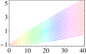
$E/(\omega_{o}j)$	$\Delta E$
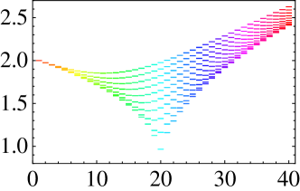
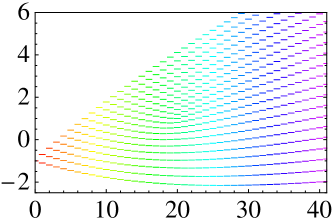
$E/(\omega_{o}j)$	$\Delta E$
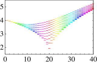
$\lambda$	$\lambda$

Figure 1: (Color online) Energy (left) and energy difference (right) as functions of $\lambda$. The parameters are $j=10$, $n_{max}=10$, $\lambda_{max}=60$, $\omega=\omega_{0}=1$, $\gamma=\gamma_{c}$ (above) and $\gamma=2\gamma_{c}$ (below)

Employing the semi-classical approximation to the density of states for a given energy,

$$\nu(E)=\frac{1}{(2\pi)^{2}}\int dq\,dp\,d\phi\,dj_{z}\,\delta(E-H_{cl}(q,p,\phi,j_{z})),$$

it is possible [see (I)] to identify two ESQPTs in the energy space. One, referred to as static, occurs at an energy $E/(\omega_{o}j)=1$ for any coupling. The second one, referred to as dynamic, takes place only in the superradiant phase at energies $E/(\omega_{o}j)=-1$. The semiclassical approximation to the density of states in the Dicke model is given by Basta1 ; Bran13

$$\frac{\omega}{2j}\nu(\epsilon)=\left\{\begin{array}[]{l}\frac{1}{\pi}\int_{y_{-}}^{y_{+}}\arccos\sqrt{\frac{2\gamma_{c}^{2}(y-\epsilon)}{\gamma^{2}(1-y^{2})}}dy,\ \ \ \ \epsilon_{0}\leq\epsilon<-1\\ \frac{\epsilon+1}{2}+\frac{1}{\pi}\int_{\epsilon}^{y_{+}}\arccos\sqrt{\frac{2\gamma_{c}^{2}(y-\epsilon)}{\gamma^{2}(1-y^{2})}}dy,\ \ \ |\epsilon|\leq 1\\ 1,\ \ \ \ \ \ \ \ \ \ \ \ \ \ \ \ \ \ \ \ \ \ \ \ \ \ \ \ \ \ \ \ \ \ \ \ \ \ \ \ \ \ \ \ \ \epsilon>1,\end{array}\right.$$ (7)

where $y_{\pm}=\left(-\frac{\gamma_{c}^{2}}{\gamma^{2}}\pm\frac{\gamma_{c}}{\gamma}\sqrt{2(\epsilon-\epsilon_{o})}\right)$, with $\epsilon_{o}\equiv-\frac{1}{2}\left(\frac{\gamma_{c}^{2}}{\gamma^{2}}+\frac{\gamma^{2}}{\gamma_{c}^{2}}\right)$, and we have defined the scaled energy $\epsilon=E/(\omega_{o}j)$. As it is discussed in (I), the singular behavior of the density of states can be related with the unstable points of the Hamiltonian classical flux. The relationship between the ESQPT and the onset of chaos is discussed in the following section.

III Regularity and chaos

To establish the onset of chaos in the classical version of the models, we use Poincaré surface sections for different couplings and energies. All the Poincaré sections shown along this contribution were obtained as follows: we solved numerically the equations of motion, Eqs.(3-6), and considered intersections of the orbits with the surface $p=0$. The intersections define a two dimensional surface in the three-dimensional space $q$-$j_{z}$-$\phi$. For given ($E,j_{z}$, $\phi$) the energy conservation, $E=H_{cl}(p=0,q,j_{z},\phi)$, gives two possible values $q_{\pm}$ for the variable $q$. We selected points corresponding to the largest $q_{\pm}$ and projected them finally in the polar plane $[1+(j_{z}/j)]$-$\phi$. For the quantum versions we use Peres lattices Per84 , which are a visual method that plays a role similar to that of the Poincaré sections in classical mechanics. The Peres lattices are very useful to study the route to chaos in quantum systems of two degrees of freedom. If a quantum system with two degrees of freedom and unperturbed Hamiltonian $H_{0}$ is integrable, a plot between the Hamiltonian eigenenergies and the respective eigenvalues of the constant of motion $I$ ( $[H_{0},I]=0$) form a lattice of regularly distributed points, because each energy level has a natural way to be labeled by the quantum number associated to $I$. When the system is perturbed, $H=H_{0}+\gamma H_{1}$ and becomes non-integrable, $I$ is not longer a conserved quantity. However, we can use the expectation values of $I$ (the Peres operator) in the energy eigenstates and plot them against the Hamiltonian eigenvalues. This choice connects the unperturbed and perturbed cases and such plots are called Peres lattices. A small perturbation does not destroy the regular lattice of the integrable case, instead a localized distortion is created in the lattice while the rest of the lattice remains regular. As the perturbation increases the irregular part of the lattice increases as well, allowing to identify in a simple way the regions with classical chaotic, regular or mixed counterpart. In this way the Peres method represents a qualitatively sensitive probe that allows to visualize the competition between regular and chaotic behavior in the quantum spectrum of a system Str09 . Moreover, the freedom in choosing the Peres operator makes it possible to focus on various properties of individual states and to closely follow the way how chaos sets in and proliferates in the system. The Peres lattices help us not only to characterize the chaotic, regular and mixed regimes in the quantum spectrum, they allow us to qualitatively identify the ESQPT’s and their properties.

$\langle J_{z}\rangle/j$

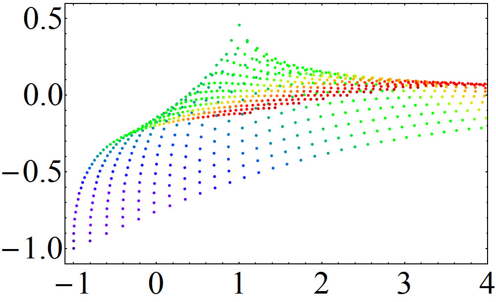
$\langle J_{z}\rangle/j$

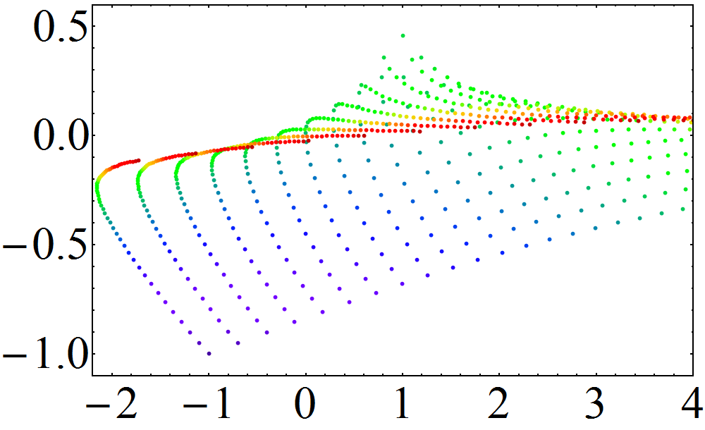
$E/(\omega_{o}j)$

Figure 2: (Color online) Peres lattices for the Tavis-Cummings model, for $\frac{\langle J_{z}\rangle}{j}$. The parameters are $j=10$, $\lambda_{max}=50$, $\omega=\omega_{0}=1$, $\gamma=\gamma_{c}$ (above) and $\gamma=2\gamma_{c}$ (below). Each color represents states with the same $\lambda$.

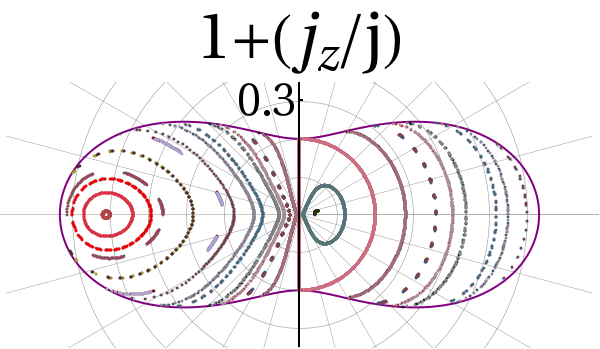
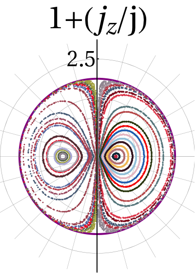
Figure 3: (Color online) Poincaré sections in polar coordinates of the pseudospin variables ($\phi$ and $1+j_{z}/j$) for the classical Tavis-Cummings model for the same couplings as fig. 2 ($\gamma=\gamma_{c}$ top row and $\gamma=2\gamma_{c}$ bottom row). The energies used are $E/(\omega_{o}j)=-0.8$ and $1.2$ for the top row, and $E/(\omega_{o}j)=-1.5$ and $1.5$ for the bottom one.

$\langle J_{z}\rangle/j$	$\langle J_{x}^{2}\rangle/j$	$\langle a^{\dagger}a\rangle/j$
$E/(\omega_{o}j)$	$E/(\omega_{o}j)$	$E/(\omega_{o}j)$

Figure 4: (Color online) Peres lattices of the Dicke model using $J_{z}$(left), $J_{x}^{2}$ (center) and $a^{\dagger}a$ (right) as Peres operators. The parameters are $j=40$, $\omega=\omega_{0}=1$, $\gamma=3\gamma_{c}$ and $N_{max}=300$ [see (I)]. Only positive parity states are considered.

Besides the Peres lattices of the quantum models, we analyze the statistical properties of their energy spectra, in different energy intervals and for different couplings. To this end we test if the energy fluctuations follow the Wigner distribution Haake , which is typical of the quantum systems with classical counterpart chaotic. The characterization is performed employing the Anderson-Darling test Anderson , which gives a simple criterion to establish if a given empirical set of data follows a given theoretical distribution. Before presenting results for the non-integrable Dicke model, the Tavis-Cummings model is discussed. In particular we focus on the signatures of the ESQPT [the abrupt changes in the DoS calculated classically in (I)] appearing in the Peres lattices of the model.

III.1 Integrable case: Tavis-Cummings

It is instructive to plot the Peres lattice for the energy $E/(\omega_{o}j)$ in the Tavis-Cummings model against the excitation number $\lambda$, displayed in Fig. 1 (left) for $\gamma=\gamma_{c}$ (up) and $\gamma=2\,\gamma_{c}$ (down), in the resonant case $\omega=\omega_{o}=1$, for a $j=10$ system. In both plots a dislocation in the regular lattice can be observed at the point with coordinates $E/(\omega_{o}j)=1$ and $\lambda=2j$ (20 in this example). It corresponds to the point in which the static excited state phase transition takes place. On the right hand side of the same figure, the energy differences between successive levels, for each value of $\lambda$, are shown. It helps to identify the point where these differences have a minimum. This is another way to recognize the presence of a singularity in the DoS, presented in (I).

When we choose $J_{z}$ as Peres operator, we obtain the Peres lattices shown in Fig.2 for two representative values of the coupling, $\gamma=\gamma_{c}$ and $\gamma=2\gamma_{c}$ in resonance $\omega=\omega_{0}=1$. It can be seen from the figure that the Peres lattices are regular (as expected due to the integrability of the TC model). In the same figure the two (static and dynamic) ESQPT are clearly evidenced by peaks in the lattices at energies $E/(\omega_{o}j)=-1$ and $1$. The ESQPT at the energy $E/(\omega_{o}j)=1$, was reported originally by Perez-Fernández et. al. Per11A and is associated to the state with $\lambda=2j$, and maximum expectation value of $\langle J_{z}\rangle$. It corresponds to the static ESQPT found in (I), when the energy is equal to that of the unstable fixed point in the north pole of the pseudospin sphere and the whole pseudospin sphere becomes accessible. This ESQPT appears for any coupling below or above $\gamma_{c}$. The other ESQPT, that takes place at $E/(\omega_{o}j)=-1$, appears only for $\gamma>\gamma_{c}$ and is associated with the state with $\lambda=0$, i.e. with no photons and no excited atoms (the ground state in the non-interacting case). From a classical point of view it corresponds to the unstable fixed point that develops at the south pole [see companion paper (I)] of the pseudospin sphere when $\gamma>\gamma_{c}$. The peaks in the lattice Peres of the TC model will be also present in the Dicke model, showing that the Peres lattices are able to detect in a visual and simple way, singular behaviors in the models. Poincaré sections for the classical version of the TC are shown in Fig. 3. As expected for the TC model, the Poincaré sections give exclusively regular orbits in accord with the regular patterns of the quantum Peres lattices.

III.2 The non-integrable Dicke model

For the Dicke model, where the $\Lambda$ symmetry of the TC model is broken, more complex Peres lattices are expected. In figure 4 we present Peres lattices for the Dicke model in the superradiant phase ($\gamma=3\gamma_{c}$), using $J_{z}$, $J^{2}_{x}$ and $a^{\dagger}a$ as Peres operators. In the three lattices a regular region in the lower part of the spectrum can be clearly identified. For energies $(E/\omega_{o}j)\approx-2$ the regularity begins to disappear and an irregular pattern is established instead. For larger energies the lattice is completely irregular. This ”route to chaos” in the quantum results, already sketched by Perez-Fernández, et. al. Per11A , has a classical correspondence as it is discussed below. Before, it is worth mentioning that, as in the case of the TC model, signatures of the static and dynamic ESQPTs are clearly seen in the lattice with $J_{z}$ as Peres operator. In the leftmost panel of Fig. 4 two peaks can be distinguished. One located around $E/(\omega_{o}j)=-1$ where $\langle J_{z}\rangle/j$ takes its lowest value, and a second one around $E/(\omega_{o}j)=1$ where $\langle J_{z}\rangle/j$ takes its largest value. The ESQPTs are related to the unstable fixed points of the classical Hamiltonian. The second peak is related to the unstable fixed point which appears for any value of the coupling where the saturation of the pseudospin variable sets in, whereas the first one corresponds to the fixed point which change from stable ($\gamma<\gamma_{c}$) to unstable at $\gamma=\gamma_{c}$.

$E/(\omega_{o}j)$

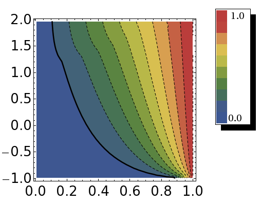
$E/(\omega_{o}j)$

$\gamma/\gamma_{c}$

Figure 5: (Color online) $v_{max}$ [see Eq.(8)] as a function of the energy and coupling for $\gamma<\gamma_{c}$ (top) and $\gamma>\gamma_{c}$ (bottom).

It is possible to understand the structure of the quantum Peres lattices from the perspective of the classical model. As it is shown in Appendix A, if we make a small oscillations approximation around the energy minimum, a quadratic Hamiltonian is obtained whose normal frequencies are given by

$$2\omega_{\pm}^{2}=\omega^{2}+\omega_{o}^{2}\pm\sqrt{(\omega_{2}^{2}-\omega_{o}^{2})^{2}+16\omega\omega_{o}\gamma^{2}},$$

for the normal phase and

$$2\gamma_{c}^{4}\omega_{\pm}^{2}=\omega_{o}^{2}\gamma^{4}+\omega^{2}\gamma_{c}^{4}\pm\sqrt{(\omega_{o}^{2}\gamma^{4}-\omega^{2}\gamma_{c}^{4})^{2}+4\omega^{2}\omega_{o}^{2}\gamma_{c}^{8}},$$

for the superradiant one. These frequencies are equal to those obtained in Ref.Emary03 by making a Holstein-Primakhof mapping of the pseudospin variables in the quantum model, likewise they were recently derived by linearizing the classical equation of motion Bakemeier13 . This latter method is completely equivalent to the one shown in Appendix A. Therefore, for energies close enough to the energy minimum, a two dimensional anisotropic harmonic oscillator is obtained with excitation eigenenergies given by $E_{n_{+},n_{-}}={n_{+}}\omega_{+}+n_{-}\omega_{-}$, with $n_{\pm}$ integer numbers equal or greater than zero. The Peres lattice of such quadratic Hamiltonian will be completely regular, and this is what it can be seen in the Peres lattices of Fig.4 for energies close to the ground-state energy. In order to obtain a rough estimate of the range of validity of the quadratic (small oscillations) approximation, we consider for a given energy ($E$) and coupling ($\gamma$), the parameter

$$v=\left|\frac{E-H_{q}(q,p,Q_{1},P_{1})}{E-E_{gs}}\right|,$$ (8)

where $H_{q}$ is the quadratic approximation of the semiclassical Hamiltonian in the normal or superradiant phase (see Appendix A), and $E_{gs}$ is the classical ground state energy for the given $\gamma$ [see Eq.(15) of companion paper (I)]. The smaller is the parameter $v$, the better is the quadratic approximation. We maximize the previous parameter in all the available phase space for a given energy $E$ and coupling $\gamma$. The results are shown in Fig.5 for the normal (top) and superradiant (bottom) phases.

As it can be seen in the figure, for very small couplings ($\gamma/\gamma_{c}\approx 0$) the quadratic approximation is valid for any energy, but for larger couplings, the range of energy where the quadratic approximation is good decreases as the coupling approaches to the critical value Hir13 . For the critical value the quadratic approximation breaks completely for any energy because the stable point around which the small oscillation expansion is made changes from stable to unstable (saddle point), and consequently one of the normal modes is equal to zero. For couplings above the critical value the quadratic approximation is valid only for a small interval above $E_{gs}$, which increases as the coupling does. In the energy intervals where the quadratic approximation is good, only regular classical orbits are expected and correspondingly a regular Peres lattice in the quantum version. For energies out of these intervals irregular or chaotic trajectories are expected to emerge. In order to visualize the way as the regular tori break as a function of energy and coupling, we use Poincare surface sections both for couplings below and above the critical one. These Poincare sections will be compared with the respective results of the quantum model.

III.3 Poincaré Sections and Peres Lattices

$\langle J_{z}\rangle/j$

$E/(\omega_{o}j)$

Figure 6: (Color online) Peres lattice $j_{z}/j$ vs $E/(\omega_{o}j)$ for a finite ($j=40$) Dicke model and a coupling $\gamma=0.2\gamma_{c}$ [a cutoff $N_{max}=160$ was used, see (I)]. In the same graph, the Anderson-Darling parameter ($A^{2}/70$, solid black line) for a test against the Wigner distribution of the Nearest Neighbor Spacings of consecutive 301 states in the spectrum, is shown as a function of the mean energy of the respective states. The horizontal dashed line indicates the maximal value ($2.5/70$) for which the test does not reject the hypothesis of a Wigner distribution for a confidence level of $95\%$.

Figure 7: (Color online) Poincaré sections ($p=0$) in the polar plane $[1+(j_{z}/j)]$-$\phi$ of the classical model for the same coupling as previous figure ($\gamma=0.2\gamma_{c}$). They correspond to energies $E/(\omega_{o}j)=-0.5$ and $2.0$.

In this subsection we make a correspondence between the Poincaré sections obtained through the semiclassical Hamiltonian, and Peres lattices attained by numerically diagonalizing Dicke Hamiltonians with $\omega=\omega_{o}=1$ and different systems sizes ($j=40$, $j=80$, and $j=100$). Convergence of the numerical results respect to the cutoff in the bosonic space ($N_{max}$) was checked as it is explained in (I). Only results for the parity positive sector of the model are presented, but similar results are obtained for the negative parity sector (see Appendix B). Likewise, we analyze the statistical properties of the quantum energy spectrum in the following way: for all the cases studied, we consider energy intervals of $N=301$ consecutive states with positive parity. Knowing the density of sates in the classical limit, it is possible to calculate the unfolded ($e_{i}$) energy spectrum Haake as $e_{i}=\Gamma_{+}(E_{i})$, with $E_{i}$ the i-th eigenenergy and $\Gamma_{+}(E)$ the cumulative energy density given by $\Gamma_{+}(E)=\int_{E_{min}}^{E}\nu_{+}(E^{\prime})dE^{\prime}$. $\nu_{+}(E)$ is the density of parity positive states, which is given by $\nu_{+}(E)=\nu(E)/2$, where $\nu(E)$ is the classical approximation to the density of states calculated in (I), and given here in Eq.(7). It is easy to prove that the differences of the unfolded energy spectrum can be approximated by $\Delta_{i}\equiv e_{i+1}-e_{i}=(1/2)\nu([E_{i+1}+E_{i}]/2)(E_{i+1}-E_{i})$. With the unfolded energy differences for a given interval ($N-1=300$ differences), we test if they follow the Wigner distribution $P_{w}(s)=(1/2)\pi se^{-\pi s^{2}/4}$, characteristic of the quantum systems with hard chaotic classical analogue. We use the statistical Anderson-Darling test Anderson which consists of calculating the so called Anderson-Darling (A-D) parameter

$$A^{2} = -(N-1)$$

$$- \sum_{k=1}^{N-1}\frac{2k-1}{N-1}\left(\ln F_{w}(\Delta_{k})+\ln[1-F_{w}(\Delta_{N-k})]\right),$$

where the $\Delta_{k}$ differences are organized in ascending order, such that $\Delta_{k}\leq\Delta_{k+1}$, and $F_{w}(s)$ is the cumulative distribution function of the Wigner distribution $F_{w}(s)=\int_{0}^{s}P_{w}(s^{\prime})ds^{\prime}$. It can be shown Anderson that if a set of data ${\Delta_{k}}$ comes from the theoretical Wigner distribution, the probability of obtaining a parameter $A^{2}$ greater than $2.5$ is 0.05 (Pr$(A^{2}>2.5)=0.05$). Then if we obtain an A-D parameter larger than 2.5 for a given set of consecutive $N$ eigenenergies, we can conclude, to a confidence level of 95 % that the statistical properties of the energy fluctuations are not described by the Wigner surmise of the quantum chaotic systems. The A-D parameter can be thought as a measure of the distance of the energy fluctuations of the Dicke energy spectrum to the Wigner distribution.

$\langle J_{z}\rangle/j$

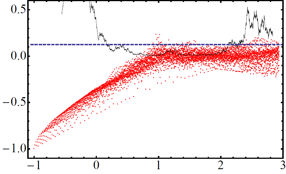
$E/(\omega_{o}j)$

Figure 8: (Color online) The same as Fig.6, for a coupling $\gamma=0.9\gamma_{c}$ and an Anderson-Darling parameter divided by 20 ($A^{2}/20$). The horizontal dashed line indicates the value $2.5/20$.

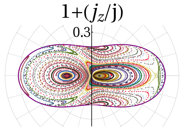
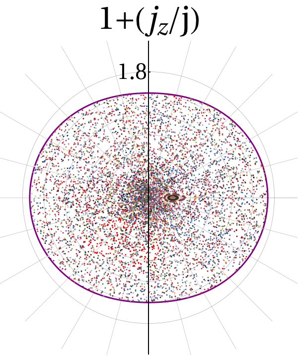
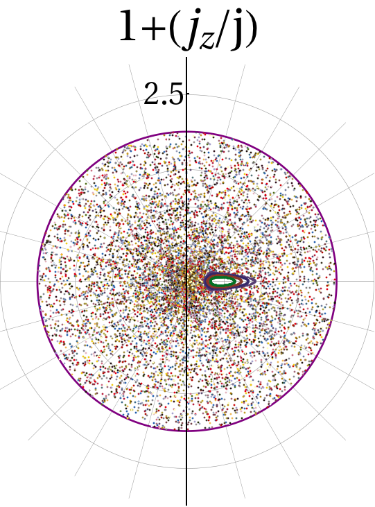
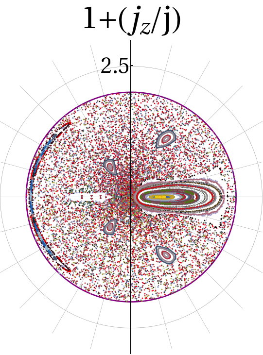
Figure 9: (Color online) Classical Poincaré sections ($p=0$) in the polar plane $[1+(j_{z}/j)]$-$\phi$ for the same system as previous figure ($\gamma=0.9\gamma_{c}$) and energies $E/(\omega_{o}j)=-0.8$, $-0.5$ (top row), $0.5$, $1.2$ (central row), and $1.8$, $2.5$ (bottom row).

We choose representative values of the coupling in order to observe several regions: the weak coupling normal phase ($\gamma=0.2\gamma_{c}$), the normal phase close to the critical value ($\gamma=0.9\gamma_{c}$), the critical coupling ($\gamma_{c}$), the superradiant phase near the critical coupling ($\gamma=1.35\gamma_{c}$), and finally, a strong coupling in the superradiant phase ($\gamma=2\gamma_{c}$)

III.3.1 Normal phase

In Fig.6 we present the Peres lattice $E$ vs $\langle J_{z}\rangle/j$ for a small coupling in the normal phase ($\gamma=0.2\gamma_{c}$). As expected according to the results of Fig 5, the Peres lattice is completely regular in every energy interval. This regularity is reflected by the A-D parameter which is greater than 2.5 for all the energy intervals. Correspondingly, the Poincaré sections of the classical model (Fig.7) show that, independent on energy, the whole phase space is filled with regular orbits. The static ESQPT that takes place at $E/(\omega_{o}j)=1$, is clearly seen in the Peres lattice as a peak located at that energy, where the expectation value $\langle J_{z}\rangle$ attains its maximal value.

Next, we increase the coupling to a value near but below the critical value ($\gamma=0.9\gamma_{c}$) where, according to Fig.5, the two modes quadratic approximation is valid only in a small interval above the energy minimum. In Fig.8 the corresponding Peres lattice is shown, where it can be observed that only in the low part of the energy spectrum a regular lattice appears, a regularity which is explained by the two modes quadratic approximation around the $E_{gs}$. For larger energies the lattice is completely irregular. The A-D parameter quantifies this change observed in the Peres lattice: for energies close to the ground states it is greater than 2.5 (rejecting, then, the hypothesis of a Wigner distribution in the energy fluctuations), and as the energy increases the A-D parameter decreases. For an energy close to $E/(\omega_{o}j)=0.2$ it attains values below $2.5$.

The corresponding Poincaré sections (Fig.9) follow closely the previous route of the quantum model. For energies close to the energy minimum, the phase space is covered only by regular orbits. As the energy increases, some regular tori break and a mixed phase space is obtained with regular and chaotic orbits. For energies $E/(\omega_{o}j)>0$ the regular tori have almost disappeared and the phase space is ergodically covered by chaotic trajectories. Interestingly, for energies around $E/(\omega_{o}j)\approx 2.5$, a revival of regular orbits is obtained in the classical model (bottom right panel of Fig.9), in correspondence this revival is also seen in the quantum model in the same energy region, where a regularity can be observed in the Peres Lattice, and the A-D parameter increases above $2.5$. The static ESQPT that takes place at energy $E/(\omega_{o}j)=1$ can be seen in the Peres lattice even if it is blurred by the quantum chaos present in this energy region. Another interesting characteristic of the Peres lattice can be seen in energies above $E/(\omega_{o}j)>1$. According to the classical analysis, for these energies the trajectories are chaotic and explore ergodically the whole pseudo-spin sphere. The quantum consequence of this classical result is that the expectation value of the operator $J_{z}$ (in fact any component of the pseudospin operator $\vec{J}$) must be equal to zero. This is what can be seen in the Peres lattice for $E/(\omega_{o}j)>1$, where the points are noticeably localized around the value $\langle J_{z}\rangle=0$.

The small oscillations approximation allows to explain the regularity observed in the low energy region both in the quantum and classical results, however the breaking of this quadratic approximation does not mean that the system is chaotic. This statement can be clearly seen in the case of the model with the thermodynamical limit critical coupling $\gamma=\gamma_{c}$. For this particular case the quadratic approximation fails for any energy because one of its normal modes is exactly zero. Even so, the Peres lattices and the classical trajectories show (Figs.10 and 11) regular patterns for energies close to the minimum, with irregular features appearing at larger energies ($E/(\omega_{o}j)\gtrsim-0.8$). The results for the critical value are very similar to those of the case $\gamma=0.9\gamma_{c}$ discussed above.

The above results show that the presence of chaos in the Dicke model is not restricted to the superradiant phase. Irregular patterns, in the classical and corresponding quantum model, appear, except in the perturbative region $\gamma\approx 0$, in the normal phase for large enough energies. The same can be said for the critical case, regularity is observed in the energy regime immediately above the energy minimum, and chaotic features are observed at larger energies.

$\langle J_{z}\rangle/j$

$E/(\omega_{o}j)$

Figure 10: (Color online) The same as Fig.6, for the critical coupling $\gamma=\gamma_{c}$ and an Anderson-Darling parameter divided by 30 ($A^{2}/30$). The horizontal dashed line indicates the value $2.5/30$.

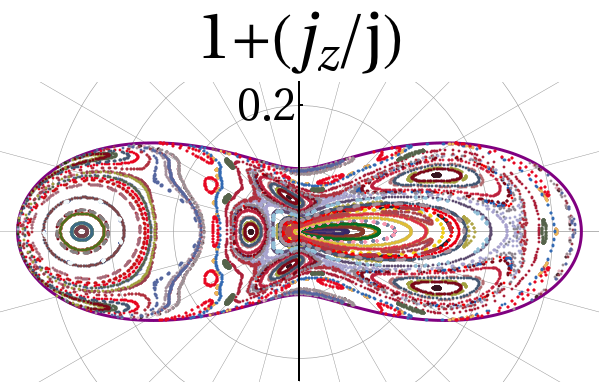
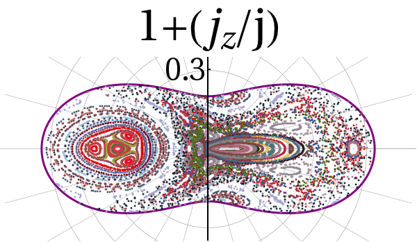
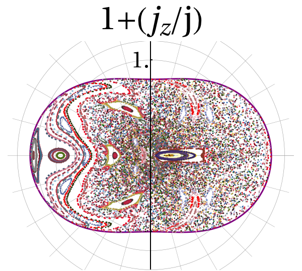
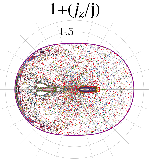
Figure 11: (Color online) Poincaré sections ($p=0$) for $\gamma=\gamma_{c}$ and energies $E/(\omega_{o}j)=-0.9$, $-0.8$ (top), and $-0.2$, $0.2$ (bottom).

III.3.2 Superradiant phase

$\langle J_{z}\rangle/j$

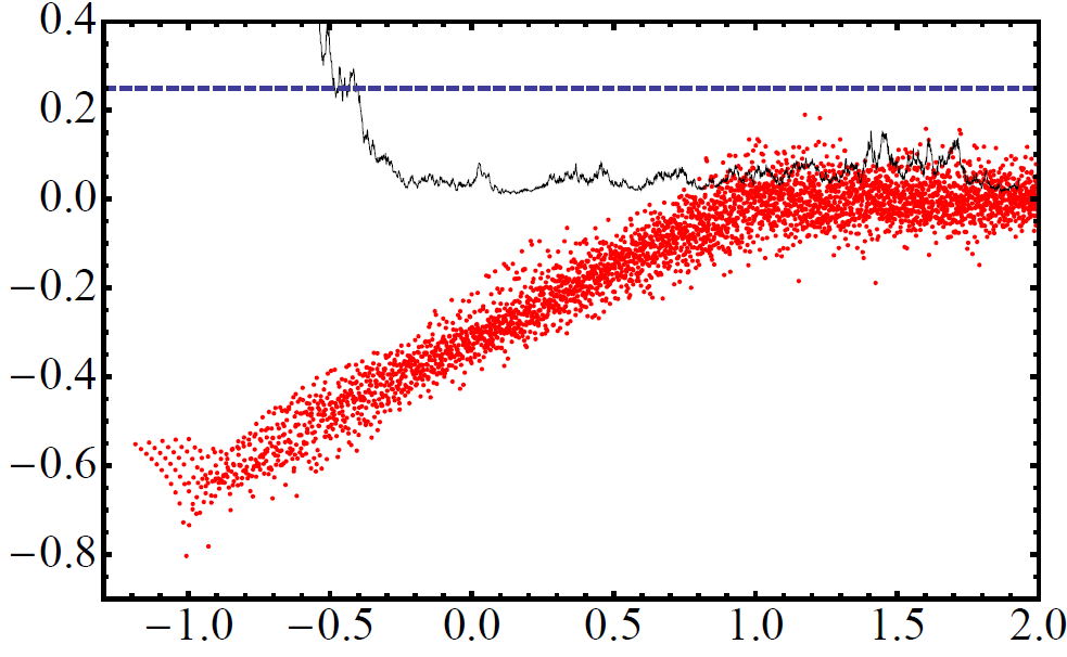
$\langle J_{z}\rangle/j$

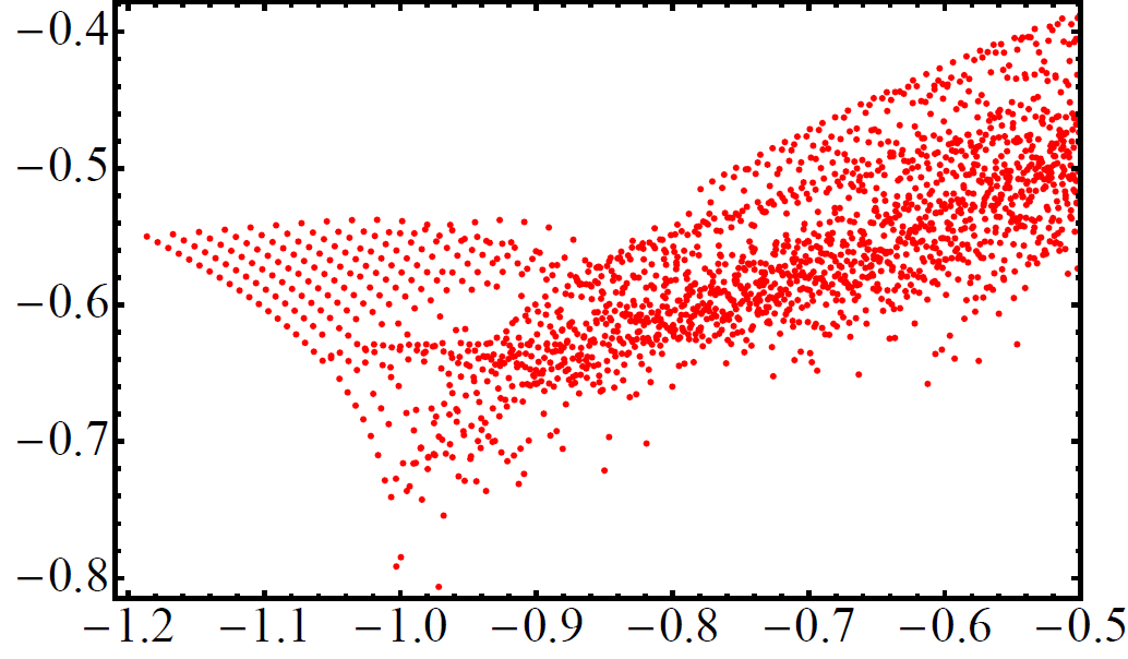
$A^{2}$

$E/(\omega_{o}j)$

Figure 12: (Color online) Top: Peres lattice for a finite system $j=40$ and coupling $\gamma/\gamma_{c}=1.35$ (a cutoff $N_{max}=160$ was used) and the Anderson-Darling parameter ($A^{2}/160$, solid black line). The horizontal dashed line indicates the maximal value ($2.5/160$) for which the test does not reject the hypothesis of a Wigner distribution for a confidence level of $95\%$. Central: A closer view of the low part of the spectrum for a larger system ($j=100$, with a cutoff $n_{max}=70$). Bottom: Anderson-Darling parameter for the system of central panel, the horizontal dashed line indicates the value $2.5$.

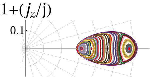
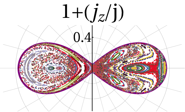
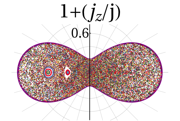
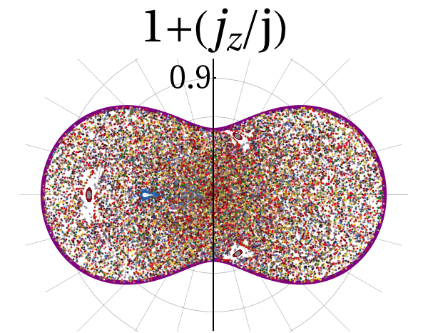
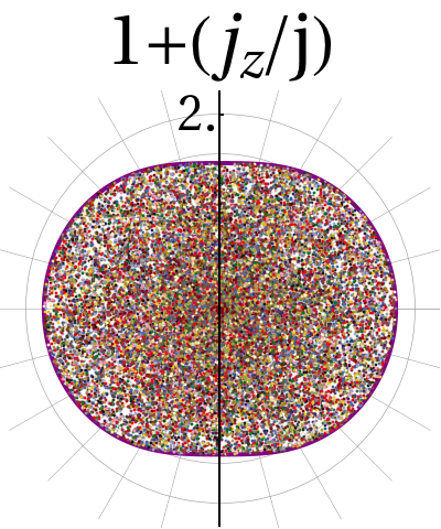
Figure 13: (Color online) Poincaré surface sections for the same system as the previous figure ($\gamma=1.35\gamma_{c}$). Every panel correspond respectively to energies $E/(\omega_{o}j)=-1.16$, $-1.0$ (top); $-0.95$, $-0.8$ (central); and $-0.5$, $0.5$ (bottom).

For couplings in the superradiant phase, a new energy region appears below the normal phase lowest energy. This new energy region corresponds, from a classical point of view, to the motion of the pseudospin variables in the double well energy surface where the parity symmetry is spontaneously broken. The top of this double well energy surface is given by the ground state energy of the normal phase ($E/(\omega_{o}j)=-1$), where the dynamical ESQPT takes place. As a first example in this coupling regime, we consider a coupling near but above the critical one $\gamma=1.35\gamma_{c}$. The corresponding Peres lattices are shown in Fig.12, whereas the classical Poincaré sections are shown in Fig.13. As it happened in the previous cases and as expected according to the Fig.5, for the low energy regime a regular lattice is obtained and correspondingly only classical regular orbits appear in the Poincaré sections. In the case of a medium size quantum system ($j=40$ top panel of Fig.12), the regular lattice seems to extend until the energy of the dynamic ESQPT ($E/(\omega_{o}j)=-1$), however a closer view of the same energy region using a larger system ($j=100$) unveils a richer structure in the denser Peres lattice: the regular lattice extends beyond the critical energy $E/(\omega_{o}j)=-1$. For a small interval around $E/(\omega_{o}j)=-1$, regular and irregular lattices coexist. For larger energies the lattice is completely irregular. These lattice characteristics are reflected by the respective A-D parameter (bottom panel of Fig.12) which decrease drastically from large values at energies close to the minimum. At $E/(\omega_{o}j)\approx-0.8$ it attains values around $A^{2}=5$, and finally at an energy $E/(\omega_{o}j)\approx-0.5$ it takes values smaller than $A^{2}=2.5$. The classical results have a clear correspondence with the quantum ones, as can be verified in the Poincaré sections of Fig. 13: regular orbits for low energies (including the critical energy $E/(\omega_{o}j)=-1$), mixed dynamics or soft chaos (coexistence of regular and chaotic trajectories) at energies near but above the critical energy $E/(\omega_{o}j)=-1$, and hard chaos (chaotic trajectories fulling the whole available phase space) for energies $E/(\omega_{o}j)\gtrsim-0.5$. The precursors of the ESQPTs, both the dynamic and static, can be clearly seen in the Peres lattice of the $j=40$ system (top panel of Fig.12), as a change in the slope of the tendency of the $\langle J_{z}\rangle$ values as the energy is increased.

$\langle J_{z}\rangle/j$

$\langle J_{z}\rangle/j$

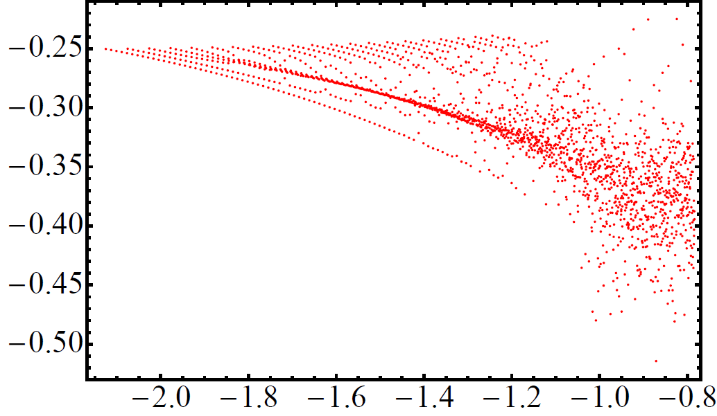
$A^{2}$

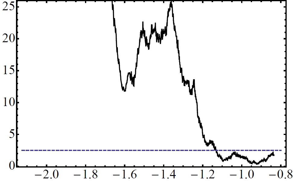
$E/(\omega_{o}j)$

Figure 14: (Color online) Top: The same as top panel of Fig.12 but for a coupling $\gamma/\gamma_{c}=2.0$ and an Anderson-Darling parameter divided by 100 ($A^{2}/100$). The horizontal dashed line indicates the value $2.5/100$. Central: Peres Lattice in a smaller energy interval for a larger system ($j=80$), the bosonic cutoff used was $N_{max}=95$. Bottom: Anderson-Darling parameter for the system of central panel, the horizontal dashed line indicates the value $2.5$.

The last case we present is one with a large coupling, deep in the superradiant phase ($\gamma=2.0\gamma_{c}$). Again, we have a regular region in the low energy sector and a hard chaotic region for higher energies. As in the previous cases the precursors of the two ESQPTs are clearly seen in the Peres lattice shown in the top panel of Fig.14. In the same panel the regular part of the lattice seems to be limited by the critical energy of the dynamic ESQPT ($E/(\omega_{o}j)=-1$), however a closer view to that energy region for a larger system ($j=80$) unveils a more involved relationship between the ESQPT and the transition to chaos. Differently to the case shown in the central panel of Fig.12 ($\gamma=1.35\gamma_{c}$, for a system size $j=100$), the regular part of the Peres lattice in this case (central panel of Fig.14) does not extend beyond $E/(\omega_{o}j)=-1$, but it is upper limited by $E/(\omega_{o}j)\approx-1.1$. For low energies the lattice is completely regular, whereas for energies around $E/(\omega_{o}j)\approx-1.1$ a coexistence of regular and irregular patterns is obtained. At the critical energy of the dynamic ESQPT the lattice seems to be completely irregular, and the same is obtained for larger energies. The previous qualitative observations are quantitatively reflected by the A-D parameter (bottom panel of Fig.14) which decrease abruptly in an energy interval around $E/(\omega_{o}j)\approx-1.1$ below the value $A^{2}=2.5$. The classical Poincaré sections (Fig. 15) present a very similar route to chaos. For $E/(\omega_{o}j)=-2.0$ only regular orbits are obtained, whereas for $E/(\omega_{o}j)=-1.4$ a mixed phase space with regular and chaotic trajectories appears. In a narrow energy interval the phase space properties change rapidly. For $E/(\omega_{o}j)=-1.2$ the chaotic trajectories fill the available phase space, excepting a small stability island, which disappears completely at larger energies.

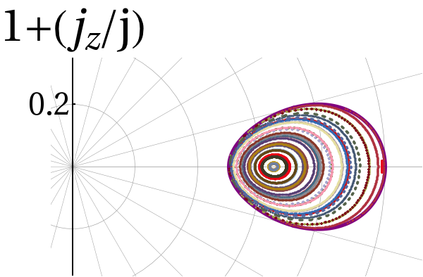
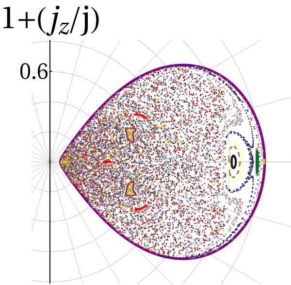
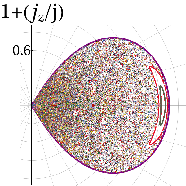
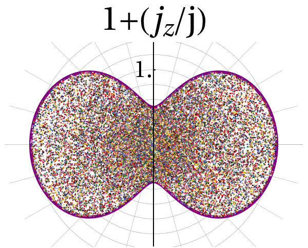
Figure 15: (Color online) Poincaré surface sections for the same system as the previous figure ($\gamma/\gamma_{c}=2.0$). Every panel correspond respectively to energies $E/(\omega_{o}j)=-2.0$,$-1.4$ (top), $-1.2$, $-1.0$ (central), and $-0.5$, $1.5$ (bottom).

The Peres lattices and the classical results which support and explain the different structures found in them, show that the change from a regular regime to a chaotic one in the Dicke model is much more involved that the transitions linked to the DoS (ESQPT) or the ground-state properties (QPT). While the ESQPT and QPT are well defined transitions in the classical limit [they are unambiguously indicated by non-analytic behavior of the ground-state energy and volume of the available phase space $\nu(E)$], the transition from a regular regime (at low energies) to a chaotic one (large energies) can not be unambiguously defined even in the classical limit. Instead continuous changes in the phase space structures are obtained, which include a mixed or soft chaos regime where regular and chaotic patterns coexist, both in the classical and quantum results, and both in the normal and superradiant phases. Nevertheless, an indirect connection between chaos and the ESQPT can be obtained through the unstable fixed points of the classical version. They determine clearly the energies where changes in the available phase space take place, and consequently singular behavior in the classical approximation of the DoS, on the other hand they are also involved in the breaking of the quadratic approximation which is a necessary (but not sufficient) condition for the presence of chaos in the classical model.

Finally, it is worth mentioning that the results presented above show that the Peres lattices are a very useful tool to explore in a qualitative and quick way the presence of chaos in the quantum models. Moreover, they are useful to give indications about the properties of the corresponding classical model. The Peres lattices allow at a glance to visualize the system properties in the energy space, contrary to the traditional Poincaré sections which are defined only for a given energy. With the Peres lattices it is easy to select individual states and identify if they are part of the regular or chaotic lattice part. In this sense they can be useful to perform more detailed studies about the classical and quantum correspondence such as the work of Ref.Bakemeier13 , where the Husimi functions of selected eigenstates are calculated and compared with the classical results. As in the present study, in that Ref. a clear quantum-classical correspondence is obtained for systems with sizes of order $\mathcal{N}\sim\mathcal{O}(10^{2})$.

IV Conclusions

Using both a semiclassical analysis and results of an efficient numerical procedure to diagonalize the quantum Hamiltonians, we have studied the Dicke and TC models in the space of coupling and energy. We focused on the onset of chaos in the non-integrable Dicke model, one of the global properties of the energy-coupling space.

We explore the properties of the quantum and classical models as a function of coupling and energy with regard to the onset of irregular patterns. Poincaré surface sections and Peres lattices were used, respectively, for the classical and quantum versions. A clear classical and quantum global correspondence was obtained for system sizes ranging from $\mathcal{N}=80$ to $200$.

Through the unstable fixed points, an indirect connection between the ESQPT’s and the onset of chaos was identified, however, the latter is a much richer phenomenon than the occurrence of non-analytic behavior in the density of states or the ground-state energy. It was found that the onset of chaos is related with the breaking of the quadratic approximation of the Hamiltonian that is obtained by considering small oscillations around the global energy minimum. It was confirmed in the quantum and classical versions, that chaos is present, both in the normal and superradiant phase, for large enough energies, except in the perturbative regime $\gamma\approx 0$. Conversely, for any coupling there always exist an energy interval above the energy minimum where only regular patterns are obtained. In particular for the very small coupling regime $\gamma\approx 0$ this energy interval extends to infinity. Once the quadratic approximation is broken more energy is needed to produce chaotic patterns, something that can be clearly seen in the classical system with critical coupling, where one of the normal modes of the quadratic approximation is exactly zero, which implies that terms of order larger than two have to be considered. Even so, the system presents regular patterns in the low energy regime, and irregular trajectories appears until larger energies. The Peres lattices used to study the quantum versions were a very useful tool to identify qualitatively the chaotic and regular features of the spectrum, moreover they show clear signatures of the ESQPTs. The qualitative information provided by the Peres lattices was quantitatively confirmed by analyzing the statistical properties of the quantum fluctuations. It was tested if the fluctuations of spectrum in different energy intervals follow the Wigner distribution characteristic of the hard chaotic systems.

The classical analysis performed in this contribution allows us to gain many insights about the results obtained in the quantum versions. For instance, it was shown that the two modes approximation obtained in Emary03 by making a Holstein-Primakhof of the pseudospin variables in the quantum model, is valid in the thermodynamic (equivalent here to the semi-classical) limit, but only for an energy region immediately above the ground-state energy. Moreover, the two modes approximation explains very well the regular patterns found in the low lying energy spectrum of the finite quantum Dicke model.

This global study may be useful as a navigation chart to more detailed studies that focus on the classical-quantum correspondence of single states, such as that performed in Ref.Bakemeier13 . Finally, the results presented here for optical models confirm results of previous studies, performed in the context of nuclear physics simple models Str09 ; CejStra1 ; CejStra2 , about the classical and quantum correspondence with regard to the onset of chaos in the extended energy and coupling space.

We thank P. Stránsky and P. Cejnar for many useful and interesting conversations.This work was partially supported by CONACyT- México, DGAPA-UNAM and DGDAEIA-UV through the ”2013 Internal call for strengthening academic groups” (UV-CA-320).

Appendix A Small oscillations around the energy minima

If small oscillations around the energy minimum are considered, a quadratic Hamiltonian is obtained whose normal frequencies $\omega_{\pm}$ give the low lying energy spectrum of the quantum model with excitation energies $E_{n_{+},n_{-}}=\omega_{+}n_{+}+\omega_{-}n_{-}$, with $n_{\pm}=0,1,2,..$. For couplings below the critical value the normal modes of the low energy regime can be obtained by expanding the classical Hamiltonian (II) around the global minimum $j_{z}=-j$. This expansion is easily obtained by transforming DickeBrasil the angular momentum canonical variables ($j_{z}$ and $\phi$) to $Q_{1}=\sqrt{2(j+j_{z})}\sin\phi$, $P_{1}=\sqrt{2(j+j_{z})}\cos\phi$. In terms of these variables the classical Hamiltonian (II) of the Dicke model ($\delta=1$), reads

$$H_{cl} = -\omega_{o}j+\frac{\omega_{o}}{2}(Q_{1}^{2}+P_{1}^{2})+\frac{\omega}{2}(q^{2}+p^{2})$$ (10)

$$+2\gamma qP_{1}\sqrt{1-\frac{Q_{1}^{2}+P_{1}^{2}}{4j}}.$$

By expanding the square root in the previous Hamiltonian, we obtain, to leading order, a quadratic Hamiltonian

$$H_{q}=-\omega_{o}j+\frac{\omega_{o}}{2}(Q_{1}^{2}+P_{1}^{2})+\frac{\omega}{2}(q^{2}+p^{2})+2\gamma qP_{1},$$ (11)

with normal frequencies Goldstein given by

$$2\omega_{\pm}^{2}=\omega^{2}+\omega_{o}^{2}\pm\sqrt{(\omega_{2}^{2}-\omega_{o}^{2})^{2}+16\omega\omega_{o}\gamma^{2}}.$$

For couplings larger than the critical one, two degenerate minima emerge, and the expansion has to be taken around these new minima ($q_{m}$, $p_{m}$, $\phi_{m}$, $j_{zm}$) given by Eq.(12) in the companion paper (I). The expansion until the quadratic leading terms is

$$H_{q} = E_{gs}+\frac{\omega}{2}\left[(q-q_{m})^{2}+p^{2}\right]$$

$$+ \frac{j\omega_{o}}{2}\left[\left(\frac{\gamma^{2}}{\gamma_{c}^{2}}-\frac{\gamma_{c}^{2}}{\gamma^{2}}\right)\phi^{2}+\frac{(\gamma/\gamma_{c})^{4}}{\left(\frac{\gamma^{2}}{\gamma_{c}^{2}}-\frac{\gamma_{c}^{2}}{\gamma^{2}}\right)}\left(\frac{j_{z}-j_{zm}}{j}\right)^{2}\right]$$

$$+ \frac{\sqrt{\omega\omega_{o}j}}{\sqrt{\frac{\gamma^{2}}{\gamma_{c}^{2}}-\frac{\gamma_{c}^{2}}{\gamma^{2}}}}(q-q_{m})\left(\frac{j_{z}-j_{zm}}{j}\right).$$

The normal modes of the previous quadratic Hamiltonian can be obtained easily Goldstein , they are

$$2\gamma_{c}^{4}\omega_{\pm}^{2}=\omega_{o}^{2}\gamma^{4}+\omega^{2}\gamma_{c}^{4}\pm\sqrt{(\omega_{o}^{2}\gamma^{4}-\omega^{2}\gamma_{c}^{4})^{2}+4\omega^{2}\omega_{o}^{2}\gamma_{c}^{8}}.$$

Appendix B Basis with defined parity

The extended bosonic basis we used in (I) to diagonalize the Dicke Hamiltonian is given Chen0809 ; Basta11 by the eigenstates of the Dicke Hamiltonian in the limit $\omega_{0}\rightarrow 0$, which are

$$|N;j,m^{\prime}\rangle\equiv\frac{1}{\sqrt{N!}}(A^{\dagger})^{N}|N=0;j,m^{\prime}\rangle,$$ (13)

where $A^{\dagger}=a^{\dagger}+\frac{2\gamma}{\sqrt{\mathcal{N}}\omega}J_{x}$, $m^{\prime}$ are the eigenvalues of $J_{x}$, and $|N=0;j,m^{\prime}\rangle=|\alpha=-\frac{2\gamma m^{\prime}}{\omega\sqrt{\mathcal{N}}}\rangle|jm^{\prime}\rangle$, with $|\alpha\rangle$ a boson coherent state and $|jm^{\prime}\rangle$ an eigenstate of the $J_{x}$ operator. The previous states are not eigenstates of the parity operator $\Pi=e^{i\pi\Lambda}=e^{i\pi(J_{z}+j)}e^{i\pi a^{\dagger}a}$. In order to analyze the statistical properties of the Dicke spectrum, we have to separate the energy eigenstates according to their parity ($p=\pm$). To this end, we construct a basis which is also an eigenbasis of the parity operator. It is easy to prove that

$$\begin{split}&|N;j,m^{\prime}\rangle=\\ &\frac{1}{\sqrt{N!}}\left(a^{\dagger}+\frac{2\gamma}{\sqrt{\mathcal{N}}\omega}m^{\prime}\right)^{N}\left|\alpha=-\frac{2\gamma m^{\prime}}{\omega\sqrt{\mathcal{N}}}\right\rangle|jm^{\prime}\rangle,\end{split}$$ (14)

this result shows that the states (13) are proportional to $|jm^{\prime}\rangle$. It can be shown (see Edmonds ) that the action of the rotation operator $e^{i\pi(J_{z}+j)}$ over $|jm^{\prime}\rangle$ gives

$$e^{i\pi(J_{z}+j)}|jm^{\prime}\rangle=|j-m^{\prime}\rangle.$$

Therefore we have

$$\begin{split}&e^{i\pi(J_{z}+j)}|N;j,m^{\prime}\rangle=\\ &\frac{1}{\sqrt{N!}}\left(a^{\dagger}+\frac{2\gamma}{\sqrt{\mathcal{N}}\omega}m^{\prime}\right)^{N}\left|\alpha=-\frac{2\gamma m^{\prime}}{\omega\sqrt{\mathcal{N}}}\right\rangle|j-m^{\prime}\rangle.\end{split}$$ (15)

On the other hand, by using the properties of the coherent states, it is straightforward to show that $e^{i\pi a^{\dagger}a}(a^{\dagger})^{k}|\alpha\rangle=(-1)^{k}(a^{\dagger})^{k}|-\alpha\rangle$. With the previous result we obtain

$$\begin{split}&e^{i\pi a^{\dagger}a}|N;j,m^{\prime}\rangle=\\ &(-1)^{N}\frac{1}{\sqrt{N!}}\left(a^{\dagger}-\frac{2\gamma}{\sqrt{\mathcal{N}}\omega}m^{\prime}\right)^{N}\left|\alpha=\frac{2\gamma m^{\prime}}{\omega\sqrt{\mathcal{N}}}\right\rangle|jm^{\prime}\rangle.\end{split}$$ (16)

By putting together Eqs.(15) and (16) we obtain

$$\Pi|N;j,m^{\prime}\rangle$$

$$=(-1)^{N}\frac{1}{\sqrt{N!}}\left(a^{\dagger}-\frac{2\gamma}{\sqrt{\mathcal{N}}\omega}m^{\prime}\right)^{N}\left|\alpha=\frac{2\gamma m^{\prime}}{\omega\sqrt{\mathcal{N}}}\right\rangle|j-m^{\prime}\rangle$$

$$=(-1)^{N}\frac{1}{\sqrt{N!}}\left(a^{\dagger}+\frac{2\gamma}{\sqrt{\mathcal{N}}\omega}J_{x}\right)^{N}\left|\alpha=\frac{2\gamma m^{\prime}}{\omega\sqrt{\mathcal{N}}}\right\rangle|j-m^{\prime}\rangle$$

$$=(-1)^{N}\frac{1}{\sqrt{N!}}(A^{\dagger})^{N}|N=0;j,-m^{\prime}\rangle=(-1)^{N}|N;j,-m^{\prime}\rangle.$$

Then, the invariant subspaces of the the parity operator are generated by states (13) with the same values $N$ and $|m^{\prime}|$. It is straightforward to diagonalize the parity operator in these subspaces, and we obtain the eigenstates of the Dicke Hamiltonian in the limit $\omega_{0}\rightarrow 0$, which are simultaneously eigenstates of the parity operator $\Pi$,

$$\begin{split}&|N;j,m^{\prime};p=\pm\rangle=\\ &=\frac{1}{\sqrt{2(1+\delta_{m^{\prime},0})}}\left(|N;j,m^{\prime}\rangle\pm(-1)^{N}|N;j,-m^{\prime}\rangle\right).\end{split}$$ (17)

Using this basis we can separate from the beginning the two parity sectors of the Dicke model and use the extended coherent basis, which has been shown Chen0809 ; Basta11 to be very efficient to study large Dicke systems.

References

- (1) R. H. Dicke, Phys. Rev. 93, 99 (1954).
- (2) K. Hepp and E. H. Lieb, Ann. Phys. (N.Y.) 76, 360 (1973).
- (3) Y. K. Wang and F. T. Hioe, Phys. Rev. A 7, 831 (1973).
- (4) Companion paper.
- (5) F. Haake, Quantum signatures of Chaos, Springer.
- (6) C. Emary and T. Brandes, Phys. Rev. E 67, 066203 (2003); Phys. Rev. Lett. 90, 044101 (2003).
- (7) P. Pérez-Fernández, A. Relaño, J. M. Arias, P. Cejnar, J. Dukelsky, and J. E. García-Ramos, Phys. Rev. E 83, 046208 (2011).
- (8) A. Altland and F. Haake, Phys. Rev. Lett. 108, 073601 (2012); New J. Phys. 14, 073011 (2012).
- (9) L. Bakemeier, A. Alvermann, and H. Fehske, Phys. Rev. A 88 043835 (2013).
- (10) E. Nahmad-Achar, O. Castaños, R. López-Peña, and J. G. Hirsch, Phys. Scr. 87 (2013) 038114.
- (11) M.A.M. de Aguiar, K. Furuya, C.H. Lewenkopf, and M.C. Nemes, Annals of Physics 216, 291 (1992).
- (12) T. Brandes, Phys. Rev. E 88, 032133 (2013).
- (13) A. Peres, Phys. Rev. Lett. 53 1711 (1984).
- (14) P.Stránský, P. Hruska, and P. Cejnar, Phys. Rev. E 79, 066201 (2009).
- (15) T.W. Anderson and D.A. Darling, Ann. Math. Statist. 23 193-212 (1952)
- (16) J. G. Hirsch, O. Castaños, E. Nahmad-Achar, and R. López-Peña, Phys. Scr. 87 (2013) 038106.
- (17) P. Cejnar and P. Stránský, Phys. Rev. Lett 93 102502 (2004)
- (18) P. Stránský, M. Kurian, and P. Cejnar, Phys. Rev. C 74 014306 (2006)
- (19) H.Goldstein, C. Poole, and J. Safko, Classical Mechanics, Addison-Wesley.
- (20) Q. H. Chen, Y. Y. Zhang, T. Liu, and K. L. Wang, Phys. Rev. A 78 051801 (2008); T. Liu, Y. Y. Zhang, Q. H. Chen, and K. L. Wang, Phys. Rev. A 80 023810 (2009).
- (21) M. A. Bastarrachea-Magnani and J. G. Hirsch, Rev. Mex. Fis. S 57 0069 (2011) http://rmf.smf.mx/pdf/rmf-s/57/3/5730069.pdf.
- (22) A. R. Edmonds, Angular Momentum in Quantum Mechanics, Princeton University Press.