Causality in Classical Physics

Abstract

Classical physics encompasses the study of physical phenomena which ranges from local (a point) to nonlocal (a region) in space and/or time. We discuss the concept of spatial and temporal nonlocality. However, one of the likely implications pertaining to nonlocality is non-causality. We study causality in the context of phenomena involving nonlocality. An appropriate domain of space and time which preserves causality is identified.

I Introduction

Classical physics (Newtonian mechanics and Maxwellian electrodynamics) deals with the space and/or time varying physical phenomena of massive point particles and the electromagnetic field. The physical happenings in classical physics are ordered in time. What ensures the correct chronological order? It is causality. Causality, in general, refers to the fact that event $E_{1}(\vec{r},t)$ must occur before in time than event $E_{2}(\vec{r}^{\prime},t^{\prime}>t)$ if $E_{1}$ influences $E_{2}$. For instance, the scalar potential $V(\vec{r},t)$ due to an arbitrarily moving point charge reads

$$V(\vec{r},t)=\frac{1}{{4\pi\varepsilon_{0}}}\int{\frac{{\rho(\vec{r}^{\prime},t-\frac{{|\vec{r}-\vec{r}^{\prime}|}}{c})}}{{|\vec{r}-\vec{r}^{\prime}|}}}d^{3}\vec{r}^{\prime};~{}(c~{}\textup{is the speed of light in vacuum.)}$$

Charge density ${\rho(\vec{r}^{\prime},t-\frac{{|\vec{r}-\vec{r}^{\prime}|}}{c})}$ as a cause precedes potential $V(\vec{r},t)$ as an observable effect. The question now arises: how long it takes for the influence to reach $E_{2}$ from $E_{1}$? The instantaneous influence from an event $E_{1}(\vec{r},t)$ to an event $E_{2}(\vec{r}^{\prime},t^{\prime})$ is not desirable from the point of view of experience. In fact, there exist a minimum time $|\vec{r}^{\prime}-\vec{r}|/c$ at which or only beyond which the disturbance in event $E_{1}(\vec{r},t)$ could be sensed by the event $E_{2}(\vec{r}^{\prime},t^{\prime})$. Causality, one of the fundamental principles of physics, requires that

• the temporal order of any two events $E_{1}(\vec{r},t)$ and $E_{2}(\vec{r}^{\prime},t^{\prime})$ must remain the same for all observers who are moving with constant velocities with respect to one another and

• the speed with which interaction can proceed between any two events $E_{1}(\vec{r},t)$ and $E_{2}(\vec{r}^{\prime},t^{\prime})$ must not exceed the speed of light in vacuum ($3\times 10^{8}ms^{-1}$).

Therefore no measurable effect can propagate from $(\vec{r},t)$ to $(\vec{r}^{\prime},t^{\prime})$ to surpass the speed of light in vacuum. Unambiguous distinction between cause and effect in the sense that cause chronologically precedes effect is thus indispensable to comply the prediction of a physical theory with the principle of causality.
Classical physics obeys the principle of locality: Newton’s equation of motion

$$m\frac{{d^{2}\vec{r}}}{{dt^{2}}}=\vec{F}(\vec{r},\dot{\vec{r}},t)$$

and Maxwell’s equations of electromagnetism

$$\vec{\nabla}.\vec{E}(\vec{r},t) = \frac{{\rho(\vec{r},t)}}{{\varepsilon_{0}}};~{}(\varepsilon_{0}~{}\textup{is electric permittivity in vacuum.})$$ (1)

$$\vec{\nabla}.\vec{B}(\vec{r},t) = 0$$ (2)

$$\vec{\nabla}\times\vec{E}(\vec{r},t) = -\frac{{\partial\vec{B}(\vec{r},t)}}{{\partial t}}$$ (3)

$$\vec{\nabla}\times\vec{B}(\vec{r},t) = \mu_{0}\vec{J}(\vec{r},t)+\frac{1}{{c^{2}}}\frac{{\partial\vec{E}(\vec{r},t)}}{{\partial t}};~{}(\mu_{0}~{}\textup{ is magnetic permeability in vacuum.)}$$ (4)

are both local. By locality we mean that an event at a given space and time can only influence the events of sufficiently nearby surroundings. Locality therefore implies that the state of a particle at time $t$ could be determined by its position $x(t)$ and its velocity $\dot{x}(t)$ alone. However, there is a subtle point buried in the mathematical definition of an instantaneous velocity $\dot{x}(t)$ with regards to causality. Velocity is defined as

$$\dot{x}(t)\equiv\frac{{dx(t)}}{{dt}}\equiv\mathop{Lt}\limits_{\Delta t\to 0}\frac{{x(t+\Delta t)-x(t)}}{{\Delta t}}$$

where ${\Delta t\to 0}$ stands for both ${\Delta t\to 0^{+}}$ and ${\Delta t\to 0^{-}}$ as $\Delta t$ can approach to zero from the right as well as from the left. Let $\Delta t\in(-\varepsilon,\varepsilon)$ where $\varepsilon$ is a small positive number. In the case when ${\Delta t\to 0^{+}}$, then $x(t+\Delta t)$ corresponds to the positions at later times compared to the position $x(t)$. The definition of an instantaneous velocity now involves the direction of the movement of position in time from future to past (as shown in FIG. 1) and thus violates causality. Whereas for ${\Delta t\to 0^{-}}$, $x(t+\Delta t)$ corresponds to the positions at earlier times with respect to the position $x(t)$. The movement of position in time in this case runs from past to future and hence favors causality.

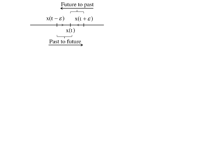
Figure 1: The right-hand derivative $\mathop{Lt}\limits_{\Delta t\to 0^{+}}\frac{{x(t+\Delta t)-x(t)}}{{\Delta t}}$ connects future to past whereas the left-hand derivative $\mathop{Lt}\limits_{\Delta t\to 0^{-}}\frac{{x(t+\Delta t)-x(t)}}{{\Delta t}}$ connects past to future.

Moreover, classical physics deals with the physical phenomena that exhibit nonlocality in the form of spread in space and/or time acquired by the physical observable. For instance, for the frequency $\omega$ dependent permittivity $\epsilon(\omega)$, electric displacement $\vec{D}$ and electric field $\vec{E}$ are connected by temporal nonlocality,

$$\vec{D}(\vec{r},t)=\int\limits_{-\infty}^{+\infty}dt^{\prime}\epsilon(\vec{r},t^{\prime})\vec{E}(\vec{r},t-t^{\prime})$$

in the sense that $\vec{D}$ has now gotten support over a region $|t-t^{\prime}|$ in time through $\vec{E}$. By nonlocality we mean that an event in addition to relatively nearby events can influence the suitabley distant events as well. Therefore, nonlocality implies that the state of a particle at time $t$ could be determined by its position $x(t)$ as well as all possible time derivatives of its position such as ($\dot{x}(t)$, $\ddot{x}(t)$, $\dddot{x}(t)$,…).

II Action-at-a distance

Interactions in classical physics (Newtonian mechanics) involve action at a distance. Action at a distance simply means that interaction could occur between any two distinct spatial points instantly. We shall illustrate the concept of action at a distance by considering two simple systems: one discrete and other continuous. Consider a system of $N$ stationary particles separated by a distance $R$ each (as shown in FIG.2(a)). Suppose the particles interact via an action at a distance of range say $R$. Action at a distance implies that the force between ith and jth particles

$$\vec{F}_{ij}=\vec{F}_{ij}\left({\vec{r}_{i}(t_{i}),\vec{r}_{j}(t_{j})}\right)_{t_{i}=t_{j}=t}$$

depends on the position of the ith particle as well as jth particle at the same time. Thus all the particles happen to interact at the same time. This could be possible provided the interaction propagates instantaneously (i.e. with infinite speed) across all possible spatial separations in the system. This is what which conflicts with causality that requires the finite speed of propagation of interaction.
Now, consider a particle of mass $m$ moving with velocity $v$ perpendicular to a uniform rigid rod collides head-on with its upper edge (please see FIG.2(b)).

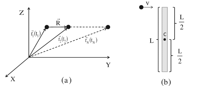
Figure 2: (a) A system of $N$ stationary particles placed at a distance $R$ each interacting via an action at a distance of range $R$. (b) A particle of mass $m$ moving with velocity $v$ strikes a uniform rod at right angle to the upper edge.

In the calculation of the velocity of the center of mass of the rod, it is implicitly assumed that the center of mass (in fact every part) of the rod senses the influence of collision at the same time the body strikes the rod and gets moved instantaneously. However, since the maximum allowable speed of the propagation of interaction is $c$, therefore, center of mass would not know as to the collision until a later time $t=L/2c$. The impulsive force (as a cause) imparted by the particle at the upper edge and velocity (as an effect) of the center of mass occur at the same time. Thus the identification of cause and effect itself becomes ambiguous.

III nonlocality and its side effect

Locality implies a single space and/or time point support whereas nonlocality is the smearing of a single space and/or time support. An observable at a given space and/or time point is said to be nonlocal if, in addition, it begins to depend upon another space and/or time point(s). Thus, nonlocality is supported over a region rather than a single space and/or time point. The generic feature of nonlocality is the presence of an infinite tower of space and/or time derivatives. A nonlocal term such as

$$A(s)A(s+l)=A(s)e^{l\frac{d}{{ds}}}A(s)=A(s)\left[{1+l\frac{d}{{ds}}+\frac{1}{2}\left({l\frac{d}{{ds}}}\right)^{2}+....}\right]A(s)$$

$$\begin{array}[]{l}\left[~{}~{}{{\rm{For~{}example,~{}Let~{}}}A(s)=e^{s}~{}\textup{then}~{}e^{l\frac{d}{{ds}}}e^{s}=\left({1+l\frac{d}{{ds}}+\frac{1}{2}\left({l\frac{d}{{ds}}}\right)^{2}+...}\right)e^{s}}\right.\\ \left.{=(1+l+\frac{1}{2}l^{2}+...)e^{s}=e^{l}e^{s}=e^{l+s}=A(s+l)}~{}~{}\right]\\ \end{array}$$

possesses an arbitrarily large number of derivatives. Furthermore, it might involve the propagation of interaction with superluminal speed (faster than the speed of light) between $s$ and $s+l$ resembling the instantaneous action at a distance over $l$. In classical physics, nonlocality in space and time generally manifests in the form of the following expression:

$$\vec{A}(\vec{r},t)=\int\limits_{-\infty}^{+\infty}{d^{3}r^{\prime}dt^{\prime}\vec{B}(}\vec{r}-\vec{r}^{\prime},t-t^{\prime})C(\vec{r}^{\prime},t^{\prime})$$ (5)

This relationship is nonlocal in both space and time because $\vec{A}$ has now picked up the dependance on the space and time points other than $\vec{r}$ and $t$. $\vec{B}(\vec{r}-\vec{r}^{\prime},t-t^{\prime})$ is an space and time nonlocal function. The above nonlocal relation becomes local when

$$\vec{B}(\vec{r}-\vec{r}^{\prime},t-t^{\prime})=\vec{B}_{0}\delta(\vec{r}-\vec{r}^{\prime})\delta(t-t^{\prime}).$$

Where $\delta(\vec{r}-\vec{r}^{\prime})$ and $\delta(t-t^{\prime})$ are Dirac delta functions. The Dirac delta function $\delta(x)(=\frac{1}{{2\pi}}\int\limits_{-\infty}^{+\infty}{e^{ikx}dk})$ is defined as follows: $\delta(x)$ is $\infty$ for $x=0$ and $0$ for $x\neq 0$. The Dirac delta function has a property that $\int\limits_{-\infty}^{+\infty}{f(x)\delta(x-a)dx=f(a)}$.
$\vec{A}$ will now turn out to have dependance only on $\vec{r}$ and $t$ as follows

$$\vec{A}(\vec{r},t)=\int\limits_{-\infty}^{+\infty}{dt^{\prime}}d^{3}r^{\prime}\vec{B}_{0}\delta(\vec{r}-\vec{r}^{\prime})\delta(t-t^{\prime})C(\vec{r}^{\prime},t^{\prime})=\vec{B}_{0}C(\vec{r},t).$$

$\vec{B}$, in general, is however not localized to a point but rather smeared in space and time. How does the nonlocality in $\vec{B}$ arise? There exists a transformation called as Fourier transformation (please see section IV) that can establish a relation between $\vec{B}(\vec{r}-\vec{r}^{\prime},t-t^{\prime})$ and its counterpart $\vec{B}(\vec{k},\omega)$ in $\vec{k}$ space and $\omega$ space. We have,

$$\vec{B}(\vec{r}-\vec{r}^{\prime},t-t^{\prime}) = \int\limits_{-\infty}^{+\infty}{\frac{d^{3}k}{(2\pi)^{3/2}}\frac{d\omega}{(2\pi)^{1/2}}\vec{B}(\vec{k},\omega)}e^{i\vec{k}.(\vec{r}-\vec{r}^{\prime})}e^{-i\omega(t-t^{\prime})}$$ (6)

$$= \vec{B}\left({-i\left({\hat{i}\frac{\partial}{{\partial x}}+\hat{j}\frac{\partial}{{\partial y}}+\hat{k}\frac{\partial}{{\partial z}}}\right),i\frac{\partial}{{\partial t}}}\right)\int\limits_{-\infty}^{+\infty}{\frac{d^{3}kd\omega}{(2\pi)^{2}}}e^{i\vec{k}.(\vec{r}-\vec{r}^{\prime})}e^{-i\omega(t-t^{\prime})}$$

$$= (2\pi)^{2}\vec{B}(-i\vec{\nabla}_{\vec{r}},i\frac{\partial}{{\partial t}})\delta(\vec{r}-\vec{r}^{\prime})\delta(t-t^{\prime})$$

The differential operator $\vec{B}(-i\vec{\nabla}_{\vec{r}},i\frac{\partial}{{\partial t}})$, in the case of nonlocal theory, involves an arbitrary large number of space and time derivatives and therefore acting on the product of Dirac delta functions $\delta(\vec{r}-\vec{r}^{\prime})\delta(t-t^{\prime})$ will smear them by enlarging their domain of support. For instance, the differential operator $e^{a\frac{\partial^{2}}{\partial x^{2}}}$ acting on $\delta(x)$ yields

$$e^{a\frac{{d^{2}}}{{dx^{2}}}}\delta(x)=e^{a\frac{{d^{2}}}{{dx^{2}}}}\int\limits_{-\infty}^{+\infty}{dk}\frac{{e^{ikx}}}{{2\pi}}=\int\limits_{-\infty}^{+\infty}{dk}e^{-ak^{2}}\frac{{e^{ikx}}}{{2\pi}}=\frac{1}{{2\sqrt{\pi a}}}e^{-\frac{{x^{2}}}{4a}}$$ (7)

Thus, a single point support $x=0$ is now enlarged to an entire domain $(-\infty,\infty)$.
One of the foreseeable implications pertaining to nonlocality is acausality. The immediate reason as to why theories involving nonlocality are vulnerable to display the symptom of causality violation could be attributed to the following facts:

• At a given point in time say $t_{0}$, interaction can take place between any two spatial points on the spatial nonlocal region exhibiting action at a spatial distance.

• At a given point in space say $\vec{r}_{0}$, temporal nonlocal connection could be establish over an entire temporal nonlocal region showing action at a temporal distance and thus indistinguishing past from future and viceversa.

The following diagrams depict the said facts.

Figure 3: (a) Nonlocal spatial region (space disc) of size $l$ on which any two points can communicate at a given instant $t_{0}$. (b) Nonlocal temporal region (time rod) of size $\tau$ for which any given spatial point say $\vec{r}_{0}$ could exist simultaneously in the past as well as in the future.

IV Spatio-temporal Nonlocality

Let us consider a pair of electric fields oscillating in space and time as follows:

$$\vec{E}_{1}=\vec{E}_{10}e^{i(\vec{k}_{1}.\vec{r}-\omega_{1}t)}=\vec{E}_{10}e^{i\phi_{1}(\vec{r},t)}$$

$$\vec{E}_{2}=\vec{E}_{20}e^{i(\vec{k}_{2}.\vec{r}-\omega_{2}t)}=\vec{E}_{20}e^{i\phi_{2}(\vec{r},t)}$$

We shall ask a question, under what condition, the two electric fields will oscillate with the same wave vector and same frequency? $\vec{E}_{1}$ and $\vec{E}_{2}$ will oscillate with the same wave vector provided

$$\vec{\nabla}\phi_{1}(\vec{r},t) = \vec{\nabla}\phi_{2}(\vec{r},t)$$

$$\Rightarrow \vec{k}_{1}=\vec{k}_{2}$$

and the same frequency provided

$$\frac{\partial}{{\partial t}}\phi_{1}(\vec{r},t) = \frac{\partial}{{\partial t}}\phi_{2}(\vec{r},t)$$

$$\Rightarrow \omega_{1}=\omega_{2}.$$

We now consider three physical quantities namely $\vec{A}$, $B$ and $\vec{C}$ that vary in space and time. Suppose these quantities describe some physical phenomenon in which the first order spatial and temporal derivatives of their phases happen to be the same. Then all the three physical quantities will have the same wave vector and frequency dependance as $\vec{A}(\vec{k},\omega)$, $B(\vec{k},\omega)$ and $\vec{C}(\vec{k},\omega)$. We wish to study the causal structure of the generic form of the ubiquitous equation

$$\vec{A}(\vec{k},\omega)=B(\vec{k},\omega)\vec{C}(\vec{k},\omega)$$ (8)

which embodies spatio-temporal nonlocality in classical physics. What is the form of spatio-temporal dependence of the above relation? Point in wave vector/frequecy space corresponds to a region in the configuration/time space: former is the reciprocal space of the latter. Such correspondence is established via Fourier transform which is based on the fact that any good function can be built out of a superposition of sine/cosine functions. The Fourier transform (FT) of $\vec{A}(\vec{r},t)$ and inverse Fourier transform (IFT) of $\vec{A}(\vec{k},\omega)$ are defined as follows:

$$FT\left[{\vec{A}(\vec{r},t)}\right] = \vec{A}(\vec{k},\omega)=\int\limits_{-\infty}^{+\infty}{\frac{dt}{(2\pi)^{1/2}}}\frac{d^{3}r}{(2\pi)^{3/2}}\vec{A}(\vec{r},t)e^{-i(\vec{k}.\vec{r}-\omega t)}$$ (9)

$$IFT\left[{\vec{A}(\vec{k},\omega)}\right] = \vec{A}(\vec{r},t)=\int\limits_{-\infty}^{+\infty}{\frac{d^{3}k}{(2\pi)^{3/2}}}\frac{d\omega}{(2\pi)^{1/2}}\vec{A}(\vec{k},\omega)e^{i(\vec{k}.\vec{r}-\omega t)}$$ (10)

Now, $\vec{A}(\vec{r},t)$ can be expressed in terms of $B$ and $\vec{C}$ to yield:

$$\vec{A}(\vec{r},t) = \frac{1}{(2\pi)^{2}}\int\limits_{-\infty}^{+\infty}{\vec{A}(\vec{k},t)e^{i\vec{k}.\vec{r}}e^{i\omega t}}d^{3}kd\omega=\frac{1}{(2\pi)^{2}}\int\limits_{-\infty}^{+\infty}{B(\vec{k},t)\vec{C}(\vec{k},t)e^{i\vec{k}.\vec{r}}e^{-i\omega t}}d^{3}kd\omega$$ (11)

$$= \frac{1}{(2\pi)^{6}}\int\limits_{-\infty}^{+\infty}{d^{3}r^{\prime}\int\limits_{-\infty}^{+\infty}{d^{3}r^{\prime\prime}}}\int\limits_{-\infty}^{+\infty}{dt^{\prime}\int\limits_{-\infty}^{+\infty}{dt^{\prime\prime}}}\int\limits_{-\infty}^{+\infty}{d^{3}kd\omega e^{i\vec{k}.(\vec{r}-\vec{r}^{\prime}-\vec{r}^{\prime\prime})}e^{i\omega(t^{\prime}+t^{\prime\prime}-t)}B(\vec{r}^{\prime},t^{\prime})\vec{C}(\vec{r}^{\prime\prime},t^{\prime\prime})}$$

$$= \int\limits_{-\infty}^{+\infty}{d^{3}r^{\prime}\int\limits_{-\infty}^{+\infty}{d^{3}r^{\prime\prime}}}\int\limits_{-\infty}^{+\infty}{dt^{\prime}\int\limits_{-\infty}^{+\infty}{dt^{\prime\prime}}}\delta(\vec{r}-\vec{r}^{\prime}-\vec{r}^{\prime\prime})\delta(t^{\prime}+t^{\prime\prime}-t)B(\vec{r}^{\prime},t^{\prime})\vec{C}(\vec{r}^{\prime\prime},t^{\prime\prime})$$

$$= \int\limits_{-\infty}^{+\infty}{d^{3}r^{\prime}\int\limits_{-\infty}^{+\infty}dt^{\prime}}B(\vec{r}^{\prime},t^{\prime})\vec{C}(\vec{r}-\vec{r}^{\prime},t-t^{\prime})$$

$\vec{A}(\vec{r},t)$ now depends on the values of $\vec{C}(\vec{r}-\vec{r}^{\prime},t-t^{\prime})$ not only at $\vec{r}$ and $t$ but in the neighborhood points of $\vec{r}^{\prime}$ and $t^{\prime}$ as well. Thus $\vec{A}(\vec{r},t)$ and $C(\vec{r}-\vec{r}^{\prime},t-t^{\prime})$ are connected by spatio-temporal nonlocality with $|\vec{r}-\vec{r}^{\prime}|$ and $|t-t^{\prime}|$ being the scales of spatial and temporal nonlocalities respectively. We shall now explore the implications of nonlocal connection between $\vec{A}$ and $\vec{C}$. We observe that

• $\vec{A}(\vec{r},t)$ can depend upon the value of $\vec{C}(\vec{r}-\vec{r}^{\prime},t-t^{\prime})$ in the future, i.e. for time $t^{\prime}>t$ which is possible since for some given observable time $t$, $t^{\prime}$ varies from $-\infty$ to $+\infty$.

• $\vec{A}(\vec{r},t)$ and $\vec{C}(\vec{r}-\vec{r}^{\prime},t-t^{\prime})$ could be connected by a signal which can propagate with speed $\frac{|\vec{r}-\vec{r}^{\prime}|}{|t-t^{\prime}|}$ greater than $c$ which seems feasible as $\frac{|\vec{r}-\vec{r}^{\prime}|}{|t-t^{\prime}|}$ could be arbitrarily large for some observable $\vec{r}$ and $t$ as both $\vec{r}^{\prime}$ and $t^{\prime}$ vary from $-\infty$ to $+\infty$.

IV.1 Spatially nonlocal domain of significance

Suppose a rapidly changing electric field with an arbitrary space and time dependance interacts with matter (such as linear dielectrics). The electric field would create a macroscopic dipole moment of the system. Suppose the polarization (dipole moment per unit volume) with the passage of time picks up the same wave number and frequency dependence as that of the electric field. In linear dielectrics, the polarization and electric field in wave vector and frequency spaces are related through the electric susceptibility as

$$\vec{P}(\vec{k},\omega)=\chi_{E}(\vec{k},\omega)\vec{E}(\vec{k},\omega)$$ (12)

which in the configuration and temporal spaces takes the following form:

$$\vec{P}(\vec{r},t)=\int\limits_{-\infty}^{+\infty}{d^{3}r^{\prime}\int\limits_{-\infty}^{+\infty}dt^{\prime}}\chi_{E}(\vec{r}-\vec{r}^{\prime},t-t^{\prime})\vec{E}(\vec{r}^{\prime},t^{\prime})$$ (13)

When the electric field $\vec{E}$ possesses a characteristic length scale such as wavelength ($\lambda$) which is comparable to or smaller than the distances between the polarization charges then the spatial nonlocal effects become significant. For $\lambda\mathbin{\lower 1.29167pt\hbox{$\buildrel<\over{\smash{\scriptstyle\sim}\vphantom{{}_{x}}}$}}l$, where $l$ is the average distance between the polarization charges, $\vec{E}$ can explore the details of the spatial structure of dipole moments (see FIG. 4). Thus, for $\lambda>>l$, spatial nonlocality is not important.

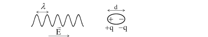
Figure 4: A macroscopic dipole moment of size $d$ created by a sinusoidal varying electric field of wavelength $\lambda$.

V Causality

How the concept of causality is implemented in classical physics? In classical physics, we often encounter the physical instances where space and/or time dependent observable effects (such as polarization $\vec{P}(\vec{r},t)$, steady state displacement $x(t)$ of the forced oscillator etc.) are caused by space and/or time dependent external perturbations (such as electric field $\vec{E}(\vec{r},t)$, time dependent force $F(t)$ etc.). The notion of causality in classical physics is implemented in the following manner:

• The physical quantity say $O(\vec{r},t)$ which appears as an observable effect must not contribute anything at time prior to the source $S(\vec{r}^{\prime},t^{\prime})$ as a cause. Thus,

  $$O(\vec{r},t)=0~{}~{}~{}~{}\textup{for}~{}~{}t<t^{\prime}$$ (14)

  Therefore, $O(\vec{r},t)$ will be nonzero only for $t>t^{\prime}$.

• The two space and time points $(\vec{r},t)$ and $(\vec{r}^{\prime},t^{\prime})$ can only be connected by a physical signal provided

  $$|\vec{r}-\vec{r}^{\prime}|~{}<~{}c|t-t^{\prime}|$$ (15)

  Therefore, $O(\vec{r},t)$ must not be different from zero for $|\vec{r}-\vec{r}^{\prime}|>c|t-t^{\prime}|$.

We now study a simple example to understand as to how to impose the condition of causality. Consider a wave packet [(continuous) superposition of monochromatic (single wavelength) waves] $\psi(x,t)$ traveling along the $x$ axis with velocity $v$ as

$$\psi_{I}(x,t)=\int\limits_{-\infty}^{+\infty}{\frac{d\omega}{(2\pi)^{1/2}}f(\omega)e^{-i\omega\left({\frac{x}{v}-t}\right)}}$$

Suppose $\psi(x,t)$ is scattered by a particle sitting at the origin. The scattered wave may be represented as

$$\psi_{S}(r,t)=\int\limits_{-\infty}^{+\infty}{\frac{d\omega}{(2\pi)^{1/2}}f(\omega)g(\omega)\frac{e^{-i\omega\left({\frac{r}{v}-t}\right)}}{r}}$$

Suppose $\psi_{I}(x,t)$ arrives at the scattering center at $t=0$ and the collision takes place in the neighborhood of time $r/v$. Then

$$\psi_{I}(0,t)=0~{}~{}~{}~{}\textup{for}~{}~{}t<0$$

with,

$$f(\omega)=\frac{1}{{(2\pi)^{1/2}}}\int\limits_{0}^{+\infty}{dt\psi_{I}(0,t)e^{i\omega t}}$$

In order to ensure causality for this process, we impose the condition that the region of integration $t<\frac{r}{v}$ should not contribute to the scattered wave packet that is

$$\psi_{S}(r,t)=0~{}~{}~{}\textup{for}~{}~{}~{}t<\frac{r}{v}$$

and

$$f(\omega)g(\omega)=\frac{1}{{(2\pi)^{1/2}}}\int\limits_{r/v}^{+\infty}{dt\psi_{S}(r,t)e^{i\omega t}}$$

Physically this means that the scattered wave packet cannot be emitted before a time $\frac{r}{v}$ unless the collision between the incident wave packet and the target takes place in the neighborhood of time $r/v$.
We now turn to our nonlocal equation. An space and time nonlocal phenomena in classical physics are generally captured by the following mathematical relation

$$\vec{A}(\vec{r},t)=\int\limits_{-\infty}^{+\infty}{d^{3}r^{\prime}\int\limits_{-\infty}^{+\infty}dt^{\prime}}B(\vec{r}-\vec{r}^{\prime},t-t^{\prime})\vec{C}(\vec{r}^{\prime},t^{\prime}).$$ (16)

Suppose $\vec{C}(\vec{r}^{\prime},t^{\prime})$ serves as a cause and $\vec{A}(\vec{r},t)$ represents an observable effect in the above equation. The causality preserving form of equation (16) could be obtained as follows. Let us shift the variable of integration $\vec{r}^{\prime}$ by $\vec{\eta}\equiv\vec{r}-\vec{r}^{\prime}$ so that equation (16) becomes

$$\vec{A}(\vec{r},t)=\int\limits_{-\infty}^{+\infty}{dt^{\prime}}\int\limits_{-\infty}^{+\infty}{d^{3}\eta}B(\vec{\eta},t-t^{\prime})\vec{C}(\vec{r}-\vec{\eta},t^{\prime})$$ (17)

where $\vec{\eta}=\vec{r}-\vec{r}^{\prime}$. Causality imposes restrictions on space and time by demanding that $\vec{A}(\vec{r},t)$ will be nonzero provided $t^{\prime}<t$ and $|\vec{\eta}|<c|t-t^{\prime}|$. Thus

$$\vec{A}_{causal}(\vec{r},t) = \int\limits_{-\infty}^{+\infty}{dt^{\prime}}\int\limits_{-\infty}^{+\infty}{d^{3}\eta}B(\vec{\eta},t-t^{\prime})\vec{C}(\vec{r}-\vec{\eta},t^{\prime})\theta(t-t^{\prime})\theta\left({c\left|{t-t^{\prime}}\right|-\left|{\vec{\eta}}\right|}\right)$$ (18)

$$= \int\limits_{-\infty}^{t}{dt^{\prime}}\int\limits_{0}^{2\pi}{d\phi}\int\limits_{0}^{\pi}{d\theta}\sin\theta\int\limits_{0}^{c|t-t^{\prime}|}{d\eta}\eta^{2}B(\vec{\eta},t-t^{\prime})\vec{C}(\vec{r}-\vec{\eta},t^{\prime})$$

where $\theta(t-t^{\prime})$ and $\theta\left({c\left|{t-t^{\prime}}\right|-\left|{\vec{\eta}}\right|}\right)$ are step functions defined by

$$\theta(t-t^{\prime}) = 1~{}~{}\textup{for}~{}~{}t>t^{\prime}~{}~{}\textup{and}~{}~{}0~{}~{}\textup{for}~{}~{}t<t^{\prime},$$

$$\theta\left({c\left|{t-t^{\prime}}\right|-\left|{\vec{\eta}}\right|}\right) = 1~{}~{}\textup{for}~{}~{}c\left|{t-t^{\prime}}\right|>\left|{\vec{\eta}}\right|~{}~{}\textup{and}~{}~{}0~{}\textup{for}~{}c\left|{t-t^{\prime}}\right|<\left|{\vec{\eta}}\right|.$$

Moreover, in the case of only temporal nonlocality , we can have

$$\vec{A}_{causal}(\vec{r},t)=\int\limits_{-\infty}^{+\infty}{dt^{\prime}}B(\vec{r},t-t^{\prime})\vec{C}(\vec{r},t^{\prime})\theta(t-t^{\prime})=\int\limits_{-\infty}^{t}{dt^{\prime}}B(\vec{r},t-t^{\prime})\vec{C}(\vec{r},t^{\prime})$$ (19)

However, for exclusively spatial nonlocality, at a given instant of time, interaction can take place between any two distinct points belonging to the region of nonlocality and hence causality is violated in the sense of action at a distance.

VI Conclusion

Non-locality is one of the crucial attributes of classical physics. However, one of the consequences of the nonlocality might be causality violation. Causality in classical physics is ensured by enforcing appropriate constraints on space and time. Unambiguous distinction between cause and effect demands cause must exist anterior to the effect as well as a signal between cause and effect can not connect by superluminal speed. The identification of causal space and time domain is therefore rather important to prevent causality violation.

SUGGESTED READING

1. J. D. Jackson, Classical Electrodynamics (New York: John Wiley $\&$ Sons, 2003), p. 330-333.

2. H. M. Nussenzveig, Causality and Dispersion Relations (New York: Academic press, 1972), p. 3-16.

3. D.I. Blokhintsev, Space and Time in the Microworld (Dordrecht-Holland: D. Reidel Publishing Company, 1973), p. 191-199.