A method for importance sampling through Markov chain Monte Carlo with post sampling variational estimate

Abstract

We propose a method to efficiently integrate truncated probability densities. The method uses Markov chain Monte Carlo method to sample from a probability density matching the function being integrated. The required normalisation or equivalently the result is obtained by constructing a function with known integral, through non-parametric kernel density estimation and variational procedure. The method is demonstrated with numerical case studies. Possible enhancements to the method and limitations are discussed.

Keywords: Markov chain Monte-Carlo, importance sampling, variational method, kernel density, hybrid Monte-Carlo, failure probability.

1 Introduction

In importance sampling Monte-Carlo methods, the variance reduction strategy is implemented by choosing a sampling density which closely mimics the function to be integrated. The new sampling density also weights the original function to correct for this introduced sampling bias [1]. Given that an optimal sampling density might exist, leads naturally to the development of algorithms, which optimize the sampling density dynamically from the past samples. These are known as adaptive importance sampling and a number of schemes have been proposed in the literature for enhancing the efficiency of importance sampling methods. These methods, variational or otherwise operate on the sampling function to optimize it, with information derived from the samples sequentially.

In this study we propose a method by which, the samples are generated exactly as per the function to be integrated (function of interest ) through Markov Chain Monte Carlo (MCMC) method. Here ’exactly’ means the sampling density differs from the function to be integrated by a constant factor. This is the condition for minimum variance  [1]. In the next step of the method, a weighting function of known integral is constructed from the samples generated in the previous step. In the third step, the integral is evaluated as an expectation of the ratio of the weighting function and function of interest or by a variational principle which minimizes the distance between the function of interest and weighting function. The steps two and three could be combined for the minimization of variance.

Though Monte-Carlo methods are useful for integration of high dimensional integrals, we demonstrate the feasibility of the proposed method by application to simple one dimensional integrals, that are typical in exceedence probability estimates. The report is organised as follows. Section 2, reviews the importance sampling Monte-Carlo principle and adaptive importance sampling methods. In section 3, the proposed method is presented. The subsections discuss the techniques such as MCMC and Kernel Density Estimation (KDE) essential in the proposed method. The use of Hybrid Monte-Carlo (HMC) for improving the performance characteristics is also presented in the subsections, as the function to be integrated has non-smooth regions. Results of numerical experiments with the proposed method is presented in section 4, where the performance is compared with direct or analogue MCS and other known importance sampling algorithms like simple importance sampling Monte-Carlo Simulation (ISMCS) and concluded in section 5.

2 Importance sampling

A number of schemes have been proposed in the literature to effect variance reduction. The following is a list of techniques  [1, 2] to name a few.

• Stratified sampling: Trial density is constructed as piecewise constant function.

• Use of negatively correlated sampling or antithetical variables

• Divide and conquer approaches: Divide the region of integration into different regions where different sampling functions can be used.

• Subset simulation: Divide and conquer strategy combined with Bayesian method, where the region of interest is represented by a sequence of subsets, whose intersection progressively results in a closer approximation to the actual domain [3].

• Variational and Bayesian adaptive importance sampling: The weighting function is adjusted by a variational method or Bayesian inference, to minimize variance [4].

• Quasi-Monte Carlo: Uses well distributed deterministic sequences instead of pseudo random numbers [2].

Importance sampling is another general and well known class of variance reduction technique. See [2, 1] for a good introduction and [5] for a recent discussion on the limitations. The general approach to importance sampling is as follows. The integral of a function $f(x)$, in the domain $[a,b]$,

$$I=\int_{a}^{b}{f(x)dx}$$ (1)

can be evaluated as an expectation of f(x), with respect to a $pdf$, $\rho(x)$ as,

$$I=\int_{a}^{b}\frac{f(x)}{\rho(x)}\rho(x)dx$$ (2)

$$=<\frac{f(x)}{\rho(x)}>_{\rho}$$ (3)

where $<f(x)>$, is the statistical expectation value

$$=\frac{1}{N}\sum_{i=1}^{N}\frac{f(x_{i})}{\rho(x_{i})}$$ (4)

There is freedom in choosing $\rho$, to generate the samples $x_{i}$. The well known variance reduction algorithms optimize $\rho$, to yield minimum variance.

The standard result in variance reduction can be obtained as in  [2], from the expression for the variance of I,

$$var(I)=\int\left[\frac{f(x)}{\rho(x)}\right]^{2}\rho(x)dx\,-\,I^{2}$$ (5)

From this equation one can infer the condition for minimum variance as,

$$f(x)\lambda=\rho(x)$$ (6)

where the constant, $\lambda=I^{-1}$. Therefore, the condition for minimum variance [2], is that the sampling density $\rho$ is a constant multiple of the function $f(x)$ to be integrated. The variance reduction principle implies that, a Monte Carlo estimate can be made more accurate for a given number of samples (or equivalently variance reduced) by sampling more frequently from the region where the function is maximum. In a sense this implies that more the information one has about the function to be integrated, smaller will be the variance.

In the next section a variant of adaptive importance sampling is proposed. Here the function to be integrated is cast as the weighting function in the integral to evaluate a function of known integral . This function of known integral is optimized with respect to the samples, to minimize variance. The new normalised function introduced takes the role of the weighting function, but the sampling is directed by the original $pdf$ whose integral is to be evaluated.

3 Post sampling variational MCS

In the field of reliability and risk analysis, it is often required to compute integrals of the form,

$$I=\int{f(x)C(x)}dx$$ (7)

Here $C(x)$ is a criteria function ($x$ could be a vector, $x\in R^{n}$), which distinguishes the success and failure domains ($\Omega_{f}$). The variables $x$ are the parameters in the dynamical system which are considered to be uncertain characterised by the $pdf$, $f(x)$. The form of $C(x)$ is,

$$C(x)=\left\{\begin{array}[]{ll}1&{when\,x\in\Omega_{f}}\\ 0&{otherwise}\end{array}\right.$$ (8)

$C(x)$ is usually implemented by a computer code. We can cast this integral as in 2 with a weighting $pdf$ , $g(x)$.

$$I=\int\left[\frac{f(x)C(x)}{g(x)}\right]g(x)dx$$ (9)

From equation 6 the condition for minimum variance implies,

$$g(x)=\lambda f(x)C(x)$$ (10)

with $\lambda=I^{-1}$. Therefore, in this equation we can minimize the variance by choosing $g(x)\sim C(x)f(x)$. i.e.,

$$g(x)=\lambda C(x)f(x)=\lambda g^{\prime}(x)$$

$\lambda$ is a normalizing constant of function $g^{\prime}(x)$, and $\frac{1}{\lambda}$gives the required probability integral of $g^{\prime}(x)$. In problems where $g^{\prime}(x)$ is known without the normalising constant, as in reliability problems ($\lambda$ is the required solution) the following approach is taken. Let h(x) be a normalised function such that $I=\int h(x)d(x)=1$. We can re-write this integral as follows,

$$I=\int\frac{h(x)}{\lambda g^{\prime}(x)}g(x)dx=1$$ (11)

with $g^{\prime}(x)$ denoting the reliability function to be integrated as, $g^{\prime}(x)=C(x)f(x)$. Rearranging 11 for $\lambda$,

$$\lambda=\int\frac{h(x)}{g^{\prime}(x)}g(x)dx$$ (12)

with the condition, $h(x)=0$ whenever $g^{\prime}(x)=0$. Therefore, $\lambda$ can be evaluated as the expectation,

$$\lambda=\left<\frac{h(x)}{g^{\prime}(x)}\right>_{g}$$ (13)

$$\lambda=\frac{1}{N}\Sigma_{i}\frac{h(x_{i})}{g^{\prime}(x_{i})}$$ (14)

Expressing the integral in this form, with the function to be chosen as $h(x)$ instead of the probability function $g(x)$, provides flexibility to optimize $h(x)$, after the samples have been chosen, and hence is referred to as post sampling variance reduction in this report.

The algorithm works as follows. Given a probability integration problem, with f(x) denoting the joint density in the input parameter space and C(x), the indicator function computed using a numerical code or analytical function,

1. generate samples from g’(x) using MCMC algorithm  [6].

2. construct a $h(x)$ which minimizes the variance of eq. 14.

3. perform the sum to evaluate $\lambda$, which is the required result.

3.1 Markov Chain Monte Carlo

The MCMC is a general method of obtaining samples from a given distribution. This method is the choice when the normalising constant of the $pdf$ of interest is unknown. A Markov chain is a stochastic process where the next state is determined only by the current state and transition probability. Given a transition rule, there is an invariant density corresponding to the Markov process defined by the transition rule. Metropolis [6] gave a prescription for obtaining the transition rule corresponding to a given $pdf$ (invariant density).

The metropolis algorithm is as follows  [7], Select an initial parameter vector $x_{0}$. Draw trial step from a symmetric pdf, i.e., $p(\Delta x)=p(-\Delta x)$
Iterate as follows: at iteration number k,

1. create new trial position $x^{\prime}=x_{k}+\Delta x$, where $\Delta x$ is randomly chosen from $p(x)$.

2. calculate the ratio $r=\frac{\pi(x^{\prime})}{\pi(x_{k})}$

3. calculate acceptance probability $\alpha=min\{1,r\}$

4. set $x_{k+1}=x^{\prime}$ with probability $\alpha$, set $x_{k+1}=x_{k}$ with probability $1-\alpha$.

Here $\pi(x)$ is the density we want to sample from and $p(x)$ is a proposal density, which is often taken as Gaussian or similar to that of the target density. Hastings generalised this procedure, by introducing non-symmetric proposals. The modified acceptance criteria, known as Metropolis-Hastings [1], is

$$\alpha=min\left\{1,\frac{\pi(x^{\prime})T(x^{\prime},x)}{\pi(x)T(x,x^{\prime})}\right\}$$ (15)

Here, T(x,x’) is the transition probability from $x$ to $x^{\prime}$. For proposals with symmetric transition probability, the above formula reduces to Metropolis acceptance criteria.

The above algorithm is referred to as symmetric random walk metropolis algorithm [8] and is easy to implement. The MCMC method may exhibit slow convergence to target distribution  [9]. This has prompted various approaches to improve convergence, such as perfect sampling, burn-in, coupling from the past, Hybrid Monte Carlo. These are some of the techniques for accelerating mixing and convergence of plain MCMC. Adapting the parametrized proposal density (transition probability) is also a line of methods known as adaptive MCMC for improving the efficiency as discussed in the next subsection.

3.2 Adaptive Importance sampling

In MCMC the proposal function can be optimized instead of manual tuning, for efficient generation of samples. The methods developed to optimize the parameters of the proposal distribution from the samples are referred to as adaptive MCMC in the literature. See for instance [8] for a discussion on optimizing parametrized transition function of MCMC. In the context of importance sampling, independent of the sampling strategy, the weighting function can also be optimized to yield minimum variance as the sampling progresses. See for instance [4] for the use of variational sampling to optimize approximations to the sampling density in the area of parameter inference. In the next section a technique for enhancing the mixing characteristics of Markov chain is discussed for use in the proposed method.

3.3 Hamiltonian Markov Chain Monte-Carlo

To improve the mixing time or burn in time of the MCMC sequence, Hamiltonian MCMC (HMC) is used in this study. This section presents the basic aspects of HMC  [9]. This method is also known as Hybrid Monte-Carlo. The first step in the method is to define an energy function (Hamiltonian) involving the variables which needs to be sampled from given distributions. In addition for each of the variables to be sampled an auxiliary variable is defined, which typically have independent Gaussian distribution. The Hamiltonian is defined as,

$$H=U(q)+K(p)$$

The kinetic energy $K(p)$, in terms of momentum variable is $=p^{2}/(2m)$. The potential energy $U(q)$ is taken as the negative logarithm of the probability density for the variables $q$.

Then, an evolution of the variables in the phase space is defined in terms of the Hamiltonian dynamics. Hamiltonian dynamics involving position like variables $q$ and momentum like variables $p$ are,

$$\frac{dq}{dt}=\frac{\partial{H}}{\partial{p}}$$ (16)

$$\frac{dp}{dt}=-\frac{\partial{H}}{\partial{q}}$$ (17)

where, $H$ is known as the Hamiltonian (Energy function). The numerical solution is obtained from the Leapfrog’s method [9], where the solutions are obtained on staggered grid, as follows,

$$p(t+\epsilon/2)=p(t)-\frac{\epsilon}{2}\frac{\partial U}{\partial q}|_{t}$$ (18)

$$q(t+\epsilon)=q(t)+\epsilon\frac{\partial K}{\partial p}|_{t+\frac{\epsilon}{2}}$$ (19)

$$p(t+\epsilon)=p(t+\frac{\epsilon}{2})-\frac{\epsilon}{2}\frac{\partial U}{\partial q}|_{t+\epsilon}$$ (20)

For the probability integral problem, the Hamiltonian energy function $H=K(p)+U(q)$ is defined as follows,

$$H(q,p)=\frac{p^{2}}{2m}-log(g(q))$$ (22)

The acceptance probability $\alpha$ for the new variables $(p^{\prime},q^{\prime})$ is,

$$\alpha=min\left\{1,\frac{exp(-H(p^{\prime},q^{\prime}))}{exp(-H(p,q))}\right\}$$

The HMC algorithm has the following steps.

1. make a new proposal as per the first step of MCMC, say $q$.

2. perform $n=\ell/\epsilon$ steps of Hamiltonian evolution with pseudo momentum $p$.

3. calculate $\alpha=exp(-(H^{\prime}-H))$. H’ is the recent Hamiltonian.

4. accept or reject the final $q^{\prime}$ as per the acceptance probability.

5. repeat the above steps.

$\ell$ and $\epsilon$ are parameters of the algorithm to be tuned for best performance. The use of HMC leads to faster convergence of MCMC sequence to the target pdf, as shown in the results subsection.

Some of the properties of Hamiltonian and its dynamics, like time reversibility, volume preservation and time invariance (energy conservation) are important for the application of Hamiltonian dynamics for MCMC [9]. The reversibility is important for showing that MCMC updates that use the dynamics leave the desired distribution invariant. The acceptance probability of proposals found by Hamilton dynamics is one, when the Hamiltonian is conserved.

Due to its slower convergence to the stationary density, plain MCMC is recommended only for special problems, where usual sampling methods cannot be applied readily. Here we apply HMC, which has better convergence properties, to simple one dimensional problems to illustrate the new approach of post adaptive sampling method. This method requires MCMC to sample from the truncated distributions appearing in reliability problems, whose normalisation constant is not known. The following section discusses the method to construct a normalised $pdf$ from MCMC or HMC samples.

3.4 Non-parametric kernel density estimators

The procedure outlined in section 3 hinges on the ability to construct a normalised function which closely matches the sampled function. One of the simplest means of constructing a pre-normalised function $h(x)$, which has the same support as the p.d.f we are interested in, is to obtain it using Kernel Density Estimator (KDE).

Given that the samples are generated from the desired distribution, kernel density estimator [10] is used to construct the density $h(x)$ as,

$$h(x,w)=\frac{1}{Nw}\sum_{j}{\phi((x-x_{j})/w)}$$ (23)

where $\phi$ being the standard normal kernel,

$$\phi(x)=\frac{1}{\sqrt{2\pi}}e^{\frac{-x^{2}}{2}}$$ (24)

$x_{j}$ are the sampled data points and $w$ a bandwidth parameter controlling the degree of smoothing. Smaller bandwidth parameter results in estimated density closely following given data and larger bandwidth more smooth estimate. Optimum $w$ is estimated using Silverman’s formula  [10].

$$w=0.9\,\sigma N^{-0.2}$$

Many methods have been suggested in the past for obtaining bandwidth estimates. The procedures may estimate a fixed $w$ or a variable $w$ [10]. When estimating variable $w$, it may be associated with $x$ or $x_{j}$ of equation 23. Further generalisation would make $w$ a matrix, increasing the complexity of KDE.

Since $h(x,w)$ must be proportional to $g\prime(x)$ for obtaining minimum variance, one can define a functional,

$$L=\sum_{i}\left[h(x_{i},w)-\lambda.g\prime(x_{i})\right]^{2}$$ (25)

for minimization with respect to the parameters $\lambda$ and $w$. In this work, $w$ is kept fixed. Solving for $\lambda$ we get,

$$\lambda=\frac{\sum_{i}h_{i}g_{i}}{\sum_{i}g_{i}^{2}}$$ (26)

$\lambda$ is identified from equation (11) as the inverse of the probability estimate. In the above expression $g\prime$ is just denoted as $g$ as it is clear from the context that only $g\prime$ is available for calculations. The expression for failure probability as given by the variational formulation (equation 26) can be compared with the expression derived directly, equation 14.

The plain KDE as in eq.  23 needs edge correction, especially if the the density being estimated is highly asymmetric near boundaries. Reflection and rescaling are two widely used methods [11] for edge correction. Both variants are tested for failure probability estimates i.e., for estimation of area under left truncated $pdf$s. In the next section we discuss the MCMC algorithm to be used for the generation of samples from $g^{\prime}(x)$.

4 Numerical experiments

The MCMC algorithm is very general for sampling applications with the added advantage that one need not know the normalising constant of the $pdf$ to generate the samples. However, there could be bias in the samples, due to initial part of the chain and may converge slowly to the target distribution. The observed bias in generating samples from uniform and normal distributions for about $10^{4}$ samples is shown in the following figures 1a and 1b respectively. The bias near the peak and right edge is shown for truncated Normal distribution in figure 1c, in linear scale and in figure 1d in log scale.

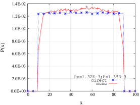
(a) Uniform distribution with 10K samples

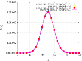
(b) Gaussian distribution with 10K samples

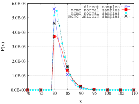
(c) Truncated Normal density, in linear scale

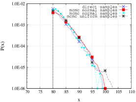
(d) Truncated Normal density, in log scale

Figure 1: Slow convergence of plain MCMC samples near peak and edges of target densities

The application of the post sampling optimization method to the integration of a known function is presented here. A Gaussian function N(0,5), mean 0, standard deviation 5, is used to check the performance of the algorithm. The table 1 presents the results for the case of variable exceeding $3\sigma$, and table 2 presents results for the case of variable exceeding $4\sigma$ level. In the tables, results from additional set of runs are given in the last three columns.

Table 1: Exceedence Probability with Post Sampling Variational Monte Carlo with HMC ($P\{x\geq\mu+3\sigma\}$).

Method	Sample size (N)	P	$\delta$	cov ($\Delta$)	P	$\delta$	cov ($\Delta$)
Analytical	-	1.349E-3	-	-	-	-	-
MCS	$2.10^{4}\times 10$	1.285E-3	-	13.3	1.390E-3	0.078	33.2
MCMC	$2.10^{4}\times 10$	1.336E-3	-	28.2	1.337E-3	0.075	31.0
IS-MCMC	$2.10^{4}\times 10$	1.43E-3	-	11.7	1.367E-3	0.017	7.3
PSV-HMC	$10^{4}\times 10$	1.337E-3	-	0.04	1.330E-3	5.5E-4	0.05

Table 2: Exceedence probability with post sampling variational Monte Carlo using HMC ($P\{x\geq\mu+4\sigma\}$)

Method	Sample size (N)	P	$\delta$	cov ($\Delta$)	P	$\delta$	cov ($\Delta$)
Analytical	-	3.1671E-5	-	-	-	-	-
MCS	$2.10^{4}\times 10$	1.0E-5	0.35	149.1	3.0E-5	0.35	149.1
MCMC	$2.10^{4}\times 10$	2.646E-5	0.097	41.1	2.83E-5	0.09	38.7
IS-MCMC	$2.10^{4}\times 10$	3.209E-5	0.016	6.62	3.131E-5	0.017	7.3
PSV-HMC	$10^{4}\times 10$	3.12E-5	4.9E-4	0.05	3.165E-5	5.1E-4	0.05

The results from Direct Monte Carlo Simulation (MCS), Simple Importance Sampling about the limit point using MCMC (IS-MCMC) and Post Sampling Adaptive (PSV-HMC) Hybrid Monte Carlo methods are compared in the tables. The IS-MCMC uses a simple weighting pdf, which is a Gaussian pdf with mean shifted to $x_{T}$ , the limit point. The $\Delta(P)$ shown in the table is known as unitary coefficient of variation and is a measure of performance of the algorithm. It is independent of number of samples $N$ but is a function of $P$. It is related to fractional error $\delta$ (also known as $cov$) as $\Delta=\delta\sqrt{N}$.

The statistical performance of the algorithm is better than simple IS Monte Carlo. It appears from the table 1, that both the importance sampling results are biased and is likely the result of the use of Markov Chain random number generator with the chains not having reached equilibrium. It is to be observed that the measure $\Delta$ does not consider the additional computation time required for constructing $h(x)$ by kernel density estimation. This makes the proposed method slower compared to direct MCS for simpler computations of $C(x)$.

The following points are to be considered while implementing the MCMC algorithm. It has been recommended in the literature that optimal acceptance ratio is about $25\%$ for MCMC algorithm. For HMC the optimal value is about $67\%$. The size of the proposal is of the order of target distribution for optimum performance and same shape as target distribution is preferred, unless the proposal distribution itself is part of the optimization.

The MCMC algorithm, though is convenient for generating random number from complex distributions, is prone to bias. The relative error and coefficient of variation metrics might present very optimistic picture statistically. While there will be still significant systematic error in the estimate.To alleviate the problem of slow convergence and bias, HMC algorithm is implemented in the study. The performance of the HMC for truncated Normal distribution is shown in figure 3. The performance without HMC is shown in figure 3 for comparison. Figure 4 presents the results for the case of exceedence limit set at 4 $\sigma$ for HMC case.

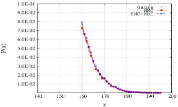
Figure 2: Convergence near peak region for truncated Normal distribution beyond 3$\sigma$, generated using HMC with edge correction.

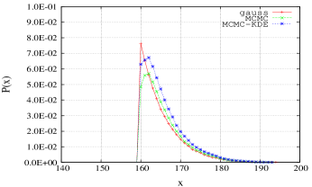
Figure 3: Slow convergence near peak region for truncated Normal distribution beyond 3$\sigma$, generated using MCMC, with edge correction.

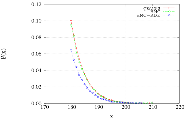
Figure 4: Convergence near peak and tail regions with HMC for truncated Normal distribution beyond 4$\sigma$ generated using HMC and edge correction.

In figures, 3 and 3 ’gauss’ or ’standard samples’ mean that the samples have been derived using python’s (programming language) Gaussian random number generator ’gauss” or analytical functions. Python uses Mersenne Twister as the core random number generator, producing 53 bit precision floats with period $2^{19937}-1$.

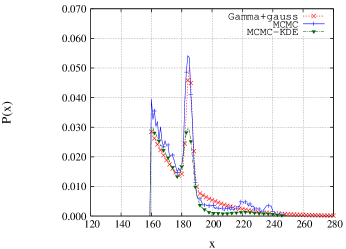
(a) Adaptive MCMC algorithm, with $10^{3}$ samples repeated 10 times

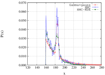
(b) Adaptive HMC algorithm, with $10^{3}$ samples repeated 10 times

Figure 5: Convergence near the truncated Gamma and Gaussian peaks using MCMC and HMC algorithms

Next the convergence of the adaptive MCMC and adaptive HMC were tested for a mixture of truncated Gamma and Gaussian distribution. The mixed distribution is obtained as,

$$g(x;\alpha,\nu)=f_{1}\frac{\alpha^{n}}{\Gamma(n)}e^{-\alpha x}x^{\nu-1}+f_{2}N(\mu,\sigma)$$

with $\alpha=0.05$, $\nu=2.5$, $\mu=185$, $\sigma=2$, $x_{T}=130$, and $f_{1}=0.998$. $N(\mu,\sigma)$ denotes normal distribution with mean $\mu$ and standard deviation $\sigma$. The convergence with adaptive MCMC is depicted in figure 5a and the convergence with adaptive HMC is shown in figure 5b. Though visually, KDE in the two figures look more or less same, quantitative results indicate better performance by HMC as seen from table 3. In this case of mixed distribution with two peaks in the domain of integration, MCS out performs ISMCS. This is due to the tail of the distribution being less skewed than the normal tail.

Table 3: Exceedence probability for mixed distribution with post sampling variational Monte Carlo using HMC ($P\{x\geq x_{T}\}$)

Method	Sample size (N)	P	$\delta$	cov ($\Delta$)	P	$\delta$	cov ($\Delta$)
Analytical	-	8.8294E-3	-	-	-	-	-
MCS	$10^{4}\times 10$	8.845E-3	0.012	3.63	8.871E-3	8.1E-4	2.5
MCMC	$10^{4}\times 10$	11.5E-3	0.132	39.7	10.857E-3	0.12	35.7
IS-MCMC	$10^{4}\times 10$	9.475E-3	0.057	16.9	8.277E-3	0.053	9.5
PSV-HMC*	$5.10^{3}\times 10$	9.33E-3	1.4E-3	0.1	9.179E-3	1.2E-3	0.1

The efficiency of the algorithm has been compared only with respect to the number of samples required by different methods. The method of using KDE entails $O(N*m)$ worst case sampling operations in one dimension, where $N$ is the number of samples in the MCMC step and $m$ is the number of samples falling within the range of the kernel density. Therefore speed up in running time will be fully realized only when the computational cost of $C(x)$ evaluation is significantly higher than the evaluation of probability densities.

5 Conclusion

A simple, and flexible algorithm for importance sampling has been presented. In this approach, the optimization problem in the evaluation of the integral is shifted to the function construction phase than at the sampling phase, which is the case in the current methods. The proposed importance sampling is quite general as there is no manual selection of matching densities in the sampling phase. The method has been tested with Gaussian and mixture of Gamma and Gaussian densities for convergence and error. The method is observed to perform better compared to well known importance sampling methods. The method’s performance can be further improved by better variational optimization strategies.

Acknowledgements: The author thanks director RDG, IGCAR, Dr. P. Chellapandi for his encouragement and support during the course of this work.

References

- [1] Jun S. liu. Monte Carlo strategies in scientific computing. Springer series in statistics. Springer-Verlag, 2001.
- [2] M. H. Kalos and P. A. Whitlock. Monte Carlo Methods. WILEY-BLACK WELL, second edition, 1997.
- [3] Siu Kui Au and James L. Beck. Estimation of small failure probabilities in high dimensions by subset simulation. Probab. Eng. Mech., 16:263–77, 2001.
- [4] Alexis Roche. Approximate inference via variational sampling. arXiv:1105.1508v2, 2011.
- [5] Nicholas J. West Laura P. Swiler. Importance sampling: Promises and limitations. In 51st AIAA/ASME/ASCE/AHS/ASC Structures, Structural Dynamics, and Materials Conference, pages 1–14, Orlando, Florida, 2010.
- [6] Metropolis N. and et al. Rosenbluth A. W. Eqautions of state calculations by fast computing machines. Journal of chemical physics, 21(6):1087–1091, 1953.
- [7] W. R. Gilks et al. Markov Chain Monte Carlo in Practice: Interdisciplinary Statistics. Chapman and Hall, New York, 1996.
- [8] C. Andrieu and J. Thoms. A tutorial on adaptive mcmc. Staistics and Computing, 18(4):343–373, 2008.
- [9] Radford. M. Neal. Mcmc using hamiltonian dynamics. In Hand Book of Markov Chain Monte-Carlo. Chapman and Hall: CRC Press, 2012.
- [10] Bruce E. Hansen. Lecture Notes on Nonparametrics. University of Wisconsin, USA, 2009.
- [11] Jones M. C. Simple boundary correction for kernel density estimation. Statistics and Computing, 3:135–146, 1993.