DESY-13-153
Precise Calculation of the Dilepton Invariant-Mass Spectrum
and the Decay Rate in $B^{\pm}\to\pi^{\pm}\mu^{+}\mu^{-}$ in the SM

Abstract

We present a precise calculation of the dilepton invariant-mass spectrum and the decay rate for $B^{\pm}\to\pi^{\pm}\ell^{+}\ell^{-}$ ($\ell^{\pm}=e^{\pm},\mu^{\pm}$) in the Standard Model (SM) based on the effective Hamiltonian approach for the $b\to d\ell^{+}\ell^{-}$ transitions. With the Wilson coefficients already known in the next-to-next-to-leading logarithmic (NNLL) accuracy, the remaining theoretical uncertainty in the short-distance contribution resides in the form factors $f_{+}(q^{2})$, $f_{0}(q^{2})$ and $f_{T}(q^{2})$. Of these, $f_{+}(q^{2})$ is well measured in the charged-current semileptonic decays $B\to\pi\ell\nu_{\ell}$ and we use the $B$-factory data to parametrize it. The corresponding form factors for the $B\to K$ transitions have been calculated in the Lattice-QCD approach for large-$q^{2}$ and extrapolated to the entire $q^{2}$-region using the so-called $z$-expansion. Using an $SU(3)_{F}$-breaking Ansatz, we calculate the $B\to\pi$ tensor form factor, which is consistent with the recently reported lattice $B\to\pi$ analysis obtained at large $q^{2}$. The prediction for the total branching fraction ${\cal B}(B^{\pm}\to\pi^{\pm}\mu^{+}\mu^{-})=(1.88^{+0.32}_{-0.21})\times 10^{-8}$ is in good agreement with the experimental value obtained by the LHCb Collaboration. In the low $q^{2}$-region, heavy-quark symmetry (HQS) relates the three form factors with each other. Accounting for the leading-order symmetry-breaking effects, and using data from the charged-current process $B\to\pi\ell\nu_{\ell}$ to determine $f_{+}(q^{2})$, we calculate the dilepton invariant-mass distribution in the low $q^{2}$-region in the $B^{\pm}\to\pi^{\pm}\ell^{+}\ell^{-}$ decay. This provides a model-independent and precise calculation of the partial branching ratio for this decay.

I Introduction

Recently, the LHCb Collaboration has reported the first observation of the $B^{\pm}\to\pi^{\pm}\mu^{+}\mu^{-}$ decay, using 1.0 fb^-1 integrated luminosity in proton-proton collisions at the Large Hadron Collider (LHC) at $\sqrt{s}=7$ TeV Aaij et al. (2012). Unlike the $b\to s\,\ell^{+}\ell^{-}$ transitions, which have been studied at the $B$-factories and hadron colliders in a number of decays, such as $B\to(K,\,K^{*})\,\ell^{+}\ell^{-}$ and $B_{s}\to\phi\,\ell^{+}\ell^{-}$ Amhis et al. (2012), the $B^{\pm}\to\pi^{\pm}\,\mu^{+}\mu^{-}$ decay is the first $b\to d\,\ell^{+}\ell^{-}$ transition measured so far. Phenomenological analysis of this process, under controlled theoretical errors, will provide us independent information concerning the $b\to d$ Flavor-Changing-Neutral-Current (FCNC) transitions in the $B$-meson sector. Hence, $B^{\pm}\to\pi^{\pm}\mu^{+}\mu^{-}$ decay is potentially an important input in the precision tests of the SM in the flavor sector and, by the same token, also in searches for physics beyond it.

The measured branching ratio ${\cal B}(B^{+}\to\pi^{+}\mu^{+}\mu^{-})=[2.3\pm 0.6({\rm stat})\pm 0.1({\rm syst})]\times 10^{-8}$ Aaij et al. (2012) is in good agreement with the SM expected rate Wang et al. (2008), which, however, like a number of other estimates in the literature Song et al. (2008); Wang and Xiao (2012), is based on model-dependent input for the $B\to\pi$ form factors. The Light-Cone Sum Rules (LCSR) approach (see, for example, Refs. Ball and Zwicky (2005) and Duplancic et al. (2008)) is certainly helpful in the low $q^{2}$-region and has been used in the current phenomenological analysis of the data Aaij et al. (2012). However, theoretical accuracy of the LCSR-based form factors is limited due to the dependence on numerous input parameters and wave-function models. Hence, it is very desirable to calculate the form factors from first principles, such as the Lattice QCD, which have their own range of validity restricted by the recoil energy (here, the energy $E_{\pi}$ of the $\pi$-meson), as the discretization errors become large with increasing $E_{\pi}$. With improved lattice technology, one can use the lattice form factors to predict the decay rates in the $B\to\pi$ and $B\to K$ transitions (as well as in other heavy-to-light meson transitions) in the low-recoil region, where the lattice results apply without any extrapolation, in a model-independent manner. At present, the dimuon invariant mass distribution in the $B^{+}\to\pi^{+}\,\mu^{+}\mu^{-}$ decay is not at hand and only the integrated branching ratio is known. We combine the lattice input with other phenomenologically robust approaches to calculate the dilepton invariant-mass spectrum in the entire $q^{2}$-region to compute the corresponding integrated decay rates for comparison with the data Aaij et al. (2012). Our framework makes use of the methods based on the heavy-quark symmetry (HQS) in the large-recoil region, data from the $B$-factory experiments on the charged-current processes $B^{0}\to\pi^{-}\ell^{+}\nu_{\ell}$ and $B^{+}\to\pi^{0}\ell^{+}\nu_{\ell}$ to determine one of the form factors, $f_{+}(q^{2})$, and the available lattice results on the $B\to\pi$ and $B\to K$ transition form factors in the low-recoil region.

We recall that the decay $B^{\pm}\to\pi^{\pm}\,\ell^{+}\ell^{-}$ involves three form factors, two of which, $f_{+}(q^{2})$ and $f_{0}(q^{2})$, characterize the hadronic $B\to\pi$ matrix element of the vector current $J_{V}^{\mu}(x)=\bar{b}(x)\gamma^{\mu}d(x)$, and the third, $f_{T}(q^{2})$, enters in the corresponding matrix element of the tensor current $J_{T}^{\mu}(x)=\bar{b}(x)\sigma^{\mu\nu}q_{\nu}d(x)$, where $q^{\mu}=p_{B}^{\mu}-p_{\pi}^{\mu}$ is the momentum transferred to the lepton pair $\ell^{+}\ell^{-}$ (see Eqs. (10) and (II) below). Using the isospin symmetry, the first two form factors are the same as the ones encountered in the charged-current processes $B^{+}\to\pi^{0}\ell^{+}\nu_{\ell}$ and $B^{0}\to\pi^{-}\ell^{+}\nu_{\ell}$. Of these, the contribution to the decay rate proportional to $f_{0}(q^{2})$ is strongly suppressed by the mass ratio $m_{\ell}^{2}/m_{B}^{2}$ (for $\ell=e,\,\mu$). The form factor $f_{+}(q^{2})$ has been well measured (modulo $|V_{ub}|$) in the entire $q^{2}$-range by the BaBar del Amo Sanchez et al. (2011a); Lees et al. (2013) and Belle Ha et al. (2011); Sibidanov et al. (2013) collaborations. We have undertaken a chi-squared fit of these data, using four popular form-factor parametrizations of $f_{+}(q^{2})$: (i) the Becirevic-Kaidalov (BK) parametrization Becirevic and Kaidalov (2000), (ii) the Ball-Zwicky (BZ) parametrization Ball and Zwicky (2005), (iii) the Boyd-Grinstein-Lebed (BGL) parametrization Boyd et al. (1995a), and (iv) the Bourrely-Caprini-Lellouch (BCL) parametrization Bourrely et al. (2009). All these parametrizations yield good fits measured in terms of $\chi^{2}_{\rm min}/{\rm ndf}$, where ndf is the number of degrees of freedom (see Table 3). However, factoring in theoretical arguments based on the Soft-Collinear Effective Theory (SCET) Becher and Hill (2006), and preference of the Lattice-QCD-based analysis of the form factors $f_{+}(q^{2})$, $f_{0}(q^{2})$, and $f_{T}(q^{2})$ in terms of the so-called $z$-expansion, and a variation thereof (see Ref. Zhou (2013) for a recent summary of the lattice heavy-to-light form factors), we use the BGL-parametrization as our preferred choice for the extraction of $f_{+}(q^{2})$ from the $B\to\pi\ell\nu_{\ell}$ data. It should be noted that our analysis for the extraction of $f_{+}(q^{2})$ is model independent as it is based on the complete set of experimental data. Meanwhile, there are also several theoretical non-perturbative methods which allows one to determine this form factor but usually in a limited $q^{2}$-range, for example the LCSRs Duplancic et al. (2008); Khodjamirian et al. (2011); Bharucha (2012) and the $k_{T}$-factorization approach Li et al. (2012), which are often invoked in estimating the vector $B\to\pi$ transition form factor.

In order to determine the other two form factors, $f_{0}(q^{2})$ and $f_{T}(q^{2})$, in the entire $q^{2}$-domain, we proceed as follows: Lattice QCD provides them in the high-$q^{2}$ region. A number of dedicated lattice-based studies of the heavy-to-light form factors are available in the literature. In particular, calculations of the form factors in the $B\to(K,\,K^{*})\,\ell^{+}\ell^{-}$ decays, based on the $(2+1)$-flavor gauge configurations generated by the MILC Collaboration Bazavov et al. (2010), have been undertaken by the FNAL/MILC Zhou et al. (2011, 2012), HPQCD Bouchard et al. (2013a, b) and the Cambridge/Edinburgh Liu et al. (2009, 2011) Lattice groups. We make use of the $B\to K$ lattice results, combining them with an Ansatz on the $SU(3)_{F}$-symmetry breaking to determine the $f_{T}(q^{2})$ form factor for the $B\to\pi$ transition. Very recently, new results on the $B\to\pi$ form factors, in particular the first preliminary results on the tensor form factor $f_{T}^{B\pi}(q^{2})$, from the lattice simulations have also become available Bouchard et al. (2013c); Du et al. (2013). While the analysis presented in Ref. Du et al. (2013) by the FermiLab Lattice and MILC Collaborations is still blinded with an unknown off-set factor, promised to be disclosed when the final results are presented, we use the available results on the $f_{T}^{BK}(q^{2})$ form factor by the HPQCD Collaboration Bouchard et al. (2013a, b) as input in the high-$q^{2}$ region to constrain our Ansatz on the $SU(3)_{F}$-symmetry breaking. Thus, combining the extraction of $f_{+}(q^{2})$ from the $B\to\pi\ell\nu_{\ell}$ data, the Lattice-QCD data on $f_{T}(q^{2})$ for the large-$q^{2}$ domain, and the BGL-like parametrization Boyd et al. (1995a) in the form of $z$-expansion to extrapolate this form factor to the lower $q^{2}$-range, we obtain the following branching ratio:

$${\cal B}(B^{+}\to\pi^{+}\mu^{+}\mu^{-})=(1.88^{+0.32}_{-0.21})\times 10^{-8}~{},$$ (1)

which has a combined accuracy of about $\pm 15$%, taking into account also the uncertainties in the CKM matrix elements, for which we have used the values obtained from the fits of the CKM unitarity triangle Beringer et al. (2012). This result is in agreement (within large experimental errors) with the experimental value reported recently by the LHCb Collaboration Aaij et al. (2012):

$${\cal B}(B^{+}\to\pi^{+}\mu^{+}\mu^{-})=\left(2.3\pm 0.6({\rm stat.})\pm 0.1({\rm syst.})\right)\times 10^{-8}.$$ (2)

As the lattice calculations of the $B\to\pi$ form factors become robust and the dilepton invariant-mass spectrum in $B^{+}\to\pi^{+}\mu^{+}\mu^{-}$ is measured, one can undertake a completely quantitative fit of the data in the SM taking into account correlations in the lattice calculations and data.

In the SM, the $b\to d\,\ell^{+}\ell^{-}$ transition is suppressed essentially by the factor $|V_{td}/V_{ts}|$ relative to the $b\to s\,\ell^{+}\ell^{-}$ transition. In terms of exclusive decays, first measurement of the ratio ${\cal B}(B^{+}\to\pi^{+}\ell^{+}\ell^{-})/{\cal B}(B^{+}\to K^{+}\ell^{+}\ell^{-})$ has been reported by the LHCb Collaboration Aaij et al. (2012):

$$\frac{{\cal B}(B^{+}\to\pi^{+}\mu^{+}\mu^{-})}{{\cal B}(B^{+}\to K^{+}\mu^{+}\mu^{-})}=0.053\pm 0.014({\rm stat.})\pm 0.001({\rm syst.})~{}.$$ (3)

In the SM, this ratio can be expressed as follows:

$$\frac{{\cal B}(B^{+}\to\pi^{+}\mu^{+}\mu^{-})}{{\cal B}(B^{+}\to K^{+}\mu^{+}\mu^{-})}=\left|\frac{V_{td}}{V_{ts}}\right|^{2}\,F^{\pi/K}_{\rm tot}~{},$$ (4)

where $F^{\pi/K}_{\rm tot}$ is the ratio resulting from the convolution of the form factors and the $q^{2}$-dependent effective Wilson coefficients. Using $F^{\pi/K}_{\rm tot}=0.87$, and neglecting the errors on this quantity, LHCb has determined the ratio of the CKM matrix elements, yielding $|V_{td}/V_{ts}|=0.266\pm 0.035({\rm stat.})\pm 0.003({\rm syst.})$ Aaij et al. (2012). At present this method is not competitive with other determinations of $|V_{td}/V_{ts}|$, such as from the $B_{(s)}-\bar{B}_{(s)}$ mixings Amhis et al. (2012), but with greatly improved statistical error, anticipated at the LHC and Super-$B$ factory experiments, this would become a valuable and independent constraint on the CKM matrix. A reliable estimate of the quantity $F^{\pi/K}_{\rm tot}$ is also required. In particular, we expect that the error on the corresponding quantity, $F^{\pi/K}_{\rm HQS}(q^{2}\leq q_{0}^{2})$, denoting the ratio of the partial branching ratios restricted to the low-$q^{2}$ domain, can be largely reduced with the help of the heavy-quark symmetry. We hope to return to improved theoretical estimates of $F^{\pi/K}_{\rm tot}$ and $F^{\pi/K}_{\rm HQS}(q^{2}\leq q_{0}^{2})$ in a future publication.

In the large-recoil limit, the form factors in the $B\to(\pi,\,\rho,\,\omega)$ and $B\to(K,\,K^{*})$ transitions obey the heavy-quark symmetry, reducing the number of independent form factors Charles et al. (1999). In particular, the $B\to\pi$ form factors $f_{0}(q^{2})$ and $f_{T}(q^{2})$ are related to $f_{+}(q^{2})$ in the HQS limit (see Eqs. (64) and (65) below). Taking into account the leading-order symmetry-breaking corrections, these relations get modified Beneke et al. (2001), bringing in their wake a dependence on the QCD coupling constant $\alpha_{s}(\mu_{h})$ and $\alpha_{s}(\mu_{hc})$, where the hard scale $\mu_{h}\simeq m_{b}$ and the intermediate (or hard-collinear) scale $\mu_{hc}=\sqrt{m_{b}\Lambda}$, with $\Lambda\simeq 0.5$ GeV, reflect the multi-scale nature of this problem. In addition, a non-perturbative quantity $\Delta F_{\pi}$, which involves the leptonic decay constants $f_{B}$ and $f_{\pi}$ and the first inverse moments of the leading-twist light-cone distribution amplitudes (LCDAs) of the $B$- and $\pi$-meson also enters (see Eqs. (VI.2) and (VI.2) below). We have used the HQS-based approach to determine the $f_{T}(q^{2})$ form factor in terms of the measured $f_{+}(q^{2})$ form factor from the semileptonic $B\to\pi\ell\nu_{\ell}$ data, discussed above. This provides a model-independent determination of the dilepton invariant-mass distribution in the low-$q^{2}$ region.

Leaving uncertainties from the form factors aside, the other main problem from the theoretical point of view in the $b\to d\,\ell^{+}\ell^{-}$ transitions is the so-called long-distance contributions, which are dominated by the $\bar{c}c$ and $\bar{u}u$ resonant states which show up as charmonia ($J/\psi$, $\psi(2S)$, $\ldots$) and light vector ($\rho$ and $\omega$) mesons, respectively. Only model-dependent descriptions (in a Breit-Wigner form) of such long-distance effects are known at present, which compromise the precision in the theoretical predictions of the total branching fractions. Excluding the resonance-dominated regions from the dilepton invariant-mass distributions is therefore the preferred way to compare data and theory. With this in mind, we calculate the following partially integrated branching ratio

$${\cal B}(B^{+}\to\pi^{+}\mu^{+}\mu^{-};\,1\,{\rm GeV}^{2}\leq q^{2}\leq 8\,{\rm GeV}^{2})$$ (5)

$$=\left(0.57^{+0.07}_{-0.05}\right)\times 10^{-8}~{},$$

where the lower and upper $q^{2}$-value boundaries are chosen to remove the light-vector ($\rho$- and $\omega$-mesons) and charmonium-resonant regions. However, with the product branching ratios Beringer et al. (2012): ${\cal B}(B^{+}\to\rho^{0}\pi^{+})\times{\cal B}(\rho^{0}\to\mu^{+}\mu^{-})=\left(3.78\pm 0.59\right)\times 10^{-10}$ and ${\cal B}(B^{+}\to\omega\pi^{+})\times{\cal B}(\omega\to\mu^{+}\mu^{-})=\left(6.2\pm 2.2\right)\times 10^{-10}$, the long-distance effects in the low-$q^{2}$ region are numerically not important.

Due to the small branching ratio, it will be a while before the entire dimuon invariant mass is completely measured in the $B^{+}\to\pi^{+}\,\mu^{+}\mu^{-}$ decay. Anticipating this, and following similar procedures adopted in the analysis of the data in the $B\to(K,\,K^{*})\,\ell^{+}\ell^{-}$ decays Bobeth et al. (2013); Hambrock and Hiller (2012) we present here results for the partial branching ratios $d{\cal B}(B^{+}\to\pi^{+}\mu^{+}\mu^{-})/dq^{2}$, binned over specified ranges $[q^{2}_{\rm min},q^{2}_{\rm max}]$ in eight $q^{2}$-intervals. They would allow the experiments to check the short-distance (renormalization-improved perturbative) part of the SM contribution in the $b\to d\,\ell^{+}\ell^{-}$ transitions precisely.

This paper is organized as follows: In Section II, we present the dilepton invariant-mass spectrum $d{\cal B}(B^{+}\to\pi^{+}\,\mu^{+}\mu^{-})/dq^{2}$ in the effective weak Hamiltonian approach based on the SM and the numerical values of the effective Wilson coefficients. Section III is devoted to the four popular parameterizations of the vector, scalar and tensor form factors. Section IV describes the fits of the semileptonic data on the $B\to\pi\ell\nu_{\ell}$ decays using the form-factor parametrizations discussed earlier. Section V describes the calculation of the form factors $f_{0}(q^{2})$ and $f_{T}(q^{2})$ for the $B\to\pi$ transition, using Lattice data as input in the high-$q^{2}$ region and the $z$-expansion to extrapolate it to low-$q^{2}$. Section VI contains the calculation of the dilepton invariant-mass spectrum in the low-$q^{2}$ region, using methods based on the heavy-quark symmetry. In Section VII, we present the dilepton invariant-mass spectrum in the entire $q^{2}$-region as well as the partial decay rates, integrated over eight different $q^{2}$-intervals. A summary and outlook are given in Section VIII.

II The $B^{+}\to\pi^{+}\ell^{+}\ell^{-}$ Decay

The effective weak Hamiltonian encompassing the transitions $b\to d\,\ell^{+}\ell^{-}$ ($\ell^{\pm}=e^{\pm}$, $\mu^{\pm}$, or $\tau^{\pm})$, in the Standard Model (SM) can be written as follows Buchalla et al. (1996):

$${\cal H}^{b\to d}_{\rm eff} = \frac{4G_{F}}{\sqrt{2}}\left[V_{ud}V_{ub}^{*}\left(C_{1}\,{\cal O}^{(u)}_{1}+C_{2}\,{\cal O}^{(u)}_{2}\right)\right.$$

$$+ \left.V_{cd}V_{cb}^{*}\left(C_{1}\,{\cal O}_{1}+C_{2}\,{\cal O}_{2}\right)-V_{td}V_{tb}^{*}\sum\limits_{i=3}^{10}C_{i}\,{\cal O}_{i}\right],$$

where $G_{F}$ is the Fermi constant, $V_{q_{1}q_{2}}$ are the CKM matrix elements which satisfy the unitary condition $V_{ud}V_{ub}^{*}+V_{cd}V_{cb}^{*}+V_{td}V_{tb}^{*}=0$ (it can be used to eliminate one combination). In contrast to the $b\to s$ transitions, all three terms in the unitarity relation are of the same order in $\lambda$ ($V_{ub}^{*}V_{ud}\sim V_{cb}^{*}V_{cd}\sim V_{tb}^{*}V_{td}\sim\lambda^{3}$), with $\lambda=\sin\theta_{12}\simeq 0.2232$ Beringer et al. (2012).

The local operators appearing in Eq. (II) are the dimension-six operators, and are defined at an arbitrary scale $\mu$ as follows Chetyrkin et al. (1997); Bobeth et al. (2000):

$${\cal O}^{(u)}_{1}=\left(\bar{d}_{L}\gamma_{\mu}T^{A}u_{L}\right)\left(\bar{u}_{L}\gamma^{\mu}T^{A}b_{L}\right),\hskip 19.91692pt$$ (7a)

$${\cal O}^{(u)}_{2}=\left(\bar{d}_{L}\gamma_{\mu}u_{L}\right)\left(\bar{u}_{L}\gamma^{\mu}b_{L}\right),$$ (7b)

$${\cal O}_{1}=\left(\bar{d}_{L}\gamma_{\mu}T^{A}c_{L}\right)\left(\bar{c}_{L}\gamma^{\mu}T^{A}b_{L}\right),\hskip 31.29802pt$$ (7c)

$${\cal O}_{2}=\left(\bar{d}_{L}\gamma_{\mu}c_{L}\right)\left(\bar{c}_{L}\gamma^{\mu}b_{L}\right),$$ (7d)

$${\cal O}_{3}=\left(\bar{d}_{L}\gamma_{\mu}b_{L}\right)\mbox{$\sum_{q}$}\left(\bar{q}\gamma^{\mu}q\right),\hskip 56.9055pt$$ (7e)

$${\cal O}_{4}=\left(\bar{d}_{L}\gamma_{\mu}T^{A}b_{L}\right)\mbox{$\sum_{q}$}\left(\bar{q}\gamma^{\mu}T^{A}q\right),$$ (7f)

$${\cal O}_{5}=\left(\bar{d}_{L}\gamma_{\mu}\gamma_{\nu}\gamma_{\rho}b_{L}\right)\mbox{$\sum_{q}$}\left(\bar{q}\gamma^{\mu}\gamma^{\nu}\gamma^{\rho}q\right),\hskip 11.38109pt$$ (7g)

$${\cal O}_{6}=\left(\bar{d}_{L}\gamma_{\mu}\gamma_{\nu}\gamma_{\rho}T^{A}b_{L}\right)\mbox{$\sum_{q}$}\left(\bar{q}\gamma^{\mu}\gamma^{\nu}\gamma^{\rho}T^{A}q\right),$$ (7h)

$${\cal O}_{7}=\frac{e\,m_{b}}{g_{\rm s}^{2}}\left(\bar{d}_{L}\sigma^{\mu\nu}b_{R}\right)F_{\mu\nu},\hskip 59.75078pt$$ (7i)

$${\cal O}_{8}=\frac{m_{b}}{g_{\rm s}}\left(\bar{d}_{L}\sigma^{\mu\nu}T^{A}b_{R}\right)G_{\mu\nu}^{A}$$ (7j)

$${\cal O}_{9}=\frac{e^{2}}{g_{\rm s}^{2}}\left(\bar{d}_{L}\gamma^{\mu}b_{L}\right)\sum_{\ell}\left(\bar{\ell}\gamma_{\mu}\ell\right),\hskip 39.83385pt$$ (7k)

$${\cal O}_{10}=\frac{e^{2}}{g_{\rm s}^{2}}\left(\bar{d}_{L}\gamma^{\mu}b_{L}\right)\sum_{\ell}\left(\bar{\ell}\gamma_{\mu}\gamma_{5}\ell\right),$$ (7l)

where $e$ is the electric elementary charge, $g_{\rm s}$ is the strong coupling, $T^{A}$ ($A=1,\ldots,N_{c}^{2}-1$) are the generators of the color $SU(N_{c})$-group with $N_{c}=3$, $\sigma_{\mu\nu}=i\left(\gamma_{\mu}\gamma_{\nu}-\gamma_{\nu}\gamma_{\mu}\right)/2$, the subscripts $L$ and $R$ refer to the left- and right-handed components of the fermion fields, $\psi_{L,R}(x)=\left(1\mp\gamma_{5}\right)\psi(x)/2$, $F_{\mu\nu}$ and $G^{A}_{\mu\nu}$ are the photon and gluon fields, respectively, and $m_{b}$ is the $b$-quark mass. (The terms in the ${\cal O}_{7}$ and ${\cal O}_{8}$ operators proportional to the $d$-quark mass $m_{d}$ are omitted as their contributions to the amplitudes are suppressed by the ratio $m_{d}/m_{b}\sim 10^{-3}$ and negligible at the present level of accuracy). Sums over $q$ and $\ell$ denote sums over all quarks (except the $t$-quark) and charged leptons, respectively.

Figure 1: Feynman diagram for the $B^{+}\to\pi^{+}\ell^{+}\ell^{-}$ decay.

The Wilson coefficients $C_{i}(\mu)$ ($i=1,\ldots,10$) depending on the renormalization scale $\mu$ are calculated at the matching scale $\mu_{W}\sim M_{W}$, the $W$-boson mass, as a perturbative expansion in the strong coupling constant $\alpha_{s}(\mu_{W})$ Bobeth et al. (2000):

$$C_{i}(\mu_{W}) = C^{(0)}_{i}(\mu_{W})+\frac{\alpha_{s}(\mu_{W})}{4\pi}\,C^{(1)}_{i}(\mu_{W})$$ (8)

$$+ \left(\frac{\alpha_{s}(\mu_{W})}{4\pi}\right)^{2}C^{(2)}_{i}(\mu_{W})+\ldots,$$

and can be evolved to a lower scale $\mu_{b}\sim m_{b}$ using the anomalous dimensions of the above operators to the NNLL order Bobeth et al. (2000):

$$\gamma_{i} = \frac{\alpha_{s}(\mu_{W})}{4\pi}\,\gamma^{(0)}_{i}+\left(\frac{\alpha_{s}(\mu_{W})}{4\pi}\right)^{2}\gamma^{(1)}_{i}$$ (9)

$$+ \left(\frac{\alpha_{s}(\mu_{W})}{4\pi}\right)^{3}\gamma^{(2)}_{i}+\ldots.$$

Feynman diagram of the $B^{+}\to\pi^{+}\ell^{+}\ell^{-}$ decay is displayed in Fig. 1 in which the solid blob represents the effective Hamiltonian ${\cal H}^{b\to d}_{\rm eff}$ (II). The hadronic matrix elements of the operators ${\cal O}_{i}$ between the $B$- and $\pi$-meson states are expressed in terms of three independent form factors $f_{+}(q^{2})$, $f_{0}(q^{2})$ and $f_{T}(q^{2})$ as follows Beneke and Feldmann (2001):

$$\langle\pi(p_{\pi})|\bar{b}\gamma^{\mu}d|B(p_{B})\rangle = f_{+}(q^{2})\left[p_{B}^{\mu}+p_{\pi}^{\mu}-\frac{m_{B}^{2}-m_{\pi}^{2}}{q^{2}}\,q^{\mu}\right]$$ (10)

$$+ f_{0}(q^{2})\,\frac{m_{B}^{2}-m_{\pi}^{2}}{q^{2}}\,q^{\mu},$$

$$\langle\pi(p_{\pi})|\bar{b}\sigma^{\mu\nu}q_{\nu}d|B(p_{B})\rangle = \frac{if_{T}(q^{2})}{m_{B}+m_{\pi}}$$

$$\times\left[q^{2}\left(p_{B}^{\mu}+p_{\pi}^{\mu}\right)-\left(m_{B}^{2}-m_{\pi}^{2}\right)q^{\mu}\right],$$

where $p_{B}^{\mu}$ and $p_{\pi}^{\mu}$ are the four-momenta of the $B$- and $\pi$-mesons, respectively, $m_{B}$ and $m_{\pi}$ are their masses, and $q^{\mu}=p_{B}^{\mu}-p_{\pi}^{\mu}$ is the momentum transferred to the lepton pair. The $B\to\pi$ transition form factors $f_{+}(q^{2})$, $f_{0}(q^{2})$ and $f_{T}(q^{2})$ are scalar functions whose shapes are determined by using non-perturbative methods. Of these, using the isospin symmetry, $f_{+}(q^{2})$ can also be obtained by performing a phenomenological analysis of the existing experimental data on the charged-current semileptonic decays $B\to\pi\ell\nu_{\ell}$. In the large-recoil (low-$q^{2}$) limit, these form factors are related by the heavy-quark symmetry, as discussed below.

The differential branching fraction in the dilepton invariant mass $q^{2}$ can be expressed as follows:

$$\frac{d{\cal B}\left(B^{+}\to\pi^{+}\ell^{+}\ell^{-}\right)}{dq^{2}} = \frac{G_{F}^{2}\alpha_{\rm em}^{2}\tau_{B}}{1024\pi^{5}m_{B}^{3}}\,|V_{tb}V_{td}^{*}|^{2}$$

$$\times \sqrt{\lambda(q^{2})}\sqrt{1-\frac{4m_{\ell}^{2}}{q^{2}}}\,F(q^{2}),$$

where $\alpha_{\rm em}$ is the fine-structure constant, $m_{\ell}$ is the lepton mass, $\tau_{B}$ is the $B$-meson lifetime,

$$\lambda(q^{2})=\left(m_{B}^{2}+m_{\pi}^{2}-q^{2}\right)^{2}-4m_{B}^{2}m_{\pi}^{2}$$ (13)

is the kinematic function encountered in three-body decays (the triangle function), and $F(q^{2})$ is the dynamical function encoding the Wilson coefficients and the form factors:

$$F(q^{2}) = \frac{2}{3}\,\lambda(q^{2})\left(1+\frac{2m_{\ell}^{2}}{q^{2}}\right)$$

$$\times \left|C_{9}^{\rm eff}(q^{2})\,f_{+}(q^{2})+\frac{2m_{b}}{m_{B}+m_{\pi}}\,C_{7}^{\rm eff}(q^{2})\,f_{T}(q^{2})\right|^{2}$$

$$+ \frac{2}{3}\,\lambda(q^{2})\left(1-\frac{4m_{\ell}^{2}}{q^{2}}\right)\left|C_{10}^{\rm eff}\,f_{+}(q^{2})\right|^{2}$$

$$+ \frac{4m_{\ell}^{2}}{q^{2}}\left(m_{B}^{2}-m_{\pi}^{2}\right)^{2}\left|C_{10}^{\rm eff}\,f_{0}(q^{2})\right|^{2}.$$

Note that the last term in Eq. (II) containing the form factor $f_{0}(q^{2})$ is strongly suppressed by the mass ratio $m_{\ell}^{2}/q^{2}$ for the electron- or muon-pair production over the most of the dilepton invariant-mass spectrum and will not be needed in our numerical estimates. The dynamical function (II) contains the effective Wilson coefficients $C_{7}^{\rm eff}(q^{2})$, $C_{9}^{\rm eff}(q^{2})$ and $C_{10}^{\rm eff}$ which are specific combinations of the Wilson coefficients entering the effective Hamiltonian (II). To the NNLO approximation, the effective Wilson coefficients are given by Bobeth et al. (2000); Asatrian et al. (2001); Asatryan et al. (2002); Ali et al. (2002); Asatrian et al. (2004):

$$C^{\rm eff}_{7}(q^{2}) = A_{7}-\frac{\alpha_{s}(\mu)}{4\pi}$$

$$\times \left[C_{1}^{(0)}F_{1}^{(7)}(s)+C_{2}^{(0)}F_{2}^{(7)}(s)+A_{8}^{(0)}F_{8}^{(7)}(s)\right]$$

$$+ \lambda_{u}\frac{\alpha_{s}(\mu)}{4\pi}\left[C_{1}^{(0)}\left(F_{1,u}^{(7)}(s)-F_{1}^{(7)}(s)\right)\right.$$

$$\hskip 31.29802pt+\left.C_{2}^{(0)}\left(F_{2,u}^{(7)}(s)-F_{2}^{(7)}(s)\right)\right],$$

$$C^{\rm eff}_{9}(q^{2}) = A_{9}+T_{9}\,h(m_{c}^{2},q^{2})$$

$$+ U_{9}\,h(m_{b}^{2},q^{2})+W_{9}\,h(0,q^{2})-\frac{\alpha_{s}(\mu)}{4\pi}$$

$$\times \left[C_{1}^{(0)}F_{1}^{(9)}(s)+C_{2}^{(0)}F_{2}^{(9)}(s)+A_{8}^{(0)}F_{8}^{(9)}(s)\right]$$

$$+ \lambda_{u}\left[\frac{4}{3}\,C_{1}+C_{2}\right]\left[h(m_{c}^{2},q^{2})-h(0,q^{2})\right]$$

$$+ \lambda_{u}\frac{\alpha_{s}(\mu)}{4\pi}\left[C_{1}^{(0)}\left(F_{1,u}^{(9)}(s)-F_{1}^{(9)}(s)\right)\right.$$

$$\hskip 31.29802pt+\left.C_{2}^{(0)}\left(F_{2,u}^{(9)}(s)-F_{2}^{(9)}(s)\right)\right],$$

$$C_{10}^{\rm eff}=\frac{4\pi}{\alpha_{s}(\mu)}\,C_{10},$$ (17)

where $s=q^{2}/m_{B}^{2}$ is the reduced momentum squared of the lepton pair. The quantity $\lambda_{u}$ above is the ratio of the CKM matrix elements, defined as follows:

$$\lambda_{u}\equiv\frac{V_{ub}V_{ud}^{*}}{V_{tb}V_{td}^{*}}=-\frac{R_{b}}{R_{t}}\,e^{i\alpha},$$ (18)

which is expressed in terms of the apex angle $\alpha$ and the sides $R_{t}=\sqrt{(1-\bar{\rho})^{2}+\bar{\eta}^{2}}$ and $R_{b}=\sqrt{\bar{\rho}^{2}+\bar{\eta}^{2}}$ Beringer et al. (2012) of the CKM unitarity triangle, where $\bar{\rho}$ and $\bar{\eta}$ are the perturbatively improved Wolfenstein parameters Wolfenstein (1983) of the CKM matrix. The usual procedure is to include an additional term usually denoted by $Y(q^{2})$ Ali et al. (2000, 2002) into the $C_{9}^{\rm eff}(q^{2})$ Wilson coefficient (II) which effectively accounts for the resonant states (mostly charmonia decaying into the lepton pair). The study of the long-distance effects based both on theoretical tools and experimental data on the two-body hadronic decays $B\to K^{(*)}+V$, where $V$ is a vector meson decaying into the lepton pair $V\to\ell^{+}\ell^{-}$, was undertaken recently in the context of the FCNC semileptonic decays $B\to K^{(*)}\ell^{+}\ell^{-}$ Khodjamirian et al. (2010, 2013); Khodjamirian (2013). The resonant contributions can be largely removed by a stringent cut, but they may have a moderate impact also away from the resonant region and are included in the analysis of the data. Similar analysis can be undertaken for the $B\to\left(\pi,\rho,\omega\right)\ell^{+}\ell^{-}$ decays also, but is not yet performed Khodjamirian (2013). We concentrate here on the short-distance part of the differential branching ratio.

Following the prescription of Ref. Ali et al. (2002), the terms $\omega_{i}(s)$ accounting for the bremsstrahlung corrections necessary for the inclusive $B\to(X_{s},\,X_{d})\,\ell^{+}\ell^{-}$ decays are omitted and, the following set of auxiliary functions is used:

$$A_{7}(\mu) = \frac{4\pi}{\alpha_{s}(\mu)}\,C_{7}(\mu)-\frac{1}{3}\,C_{3}(\mu)-\frac{4}{9}\,C_{4}(\mu)$$

$$- \frac{20}{3}\,C_{5}(\mu)-\frac{80}{9}\,C_{6}(\mu),$$

$$A_{8}(\mu) = \frac{4\pi}{\alpha_{s}(\mu)}\,C_{8}(\mu)+C_{3}(\mu)-\frac{1}{6}\,C_{4}(\mu)$$

$$+ 20\,C_{5}(\mu)-\frac{10}{3}\,C_{6}(\mu),$$

$$A_{9}(\mu) = \frac{4\pi}{\alpha_{s}(\mu)}\,C_{9}(\mu)+\sum_{i=1}^{6}C_{i}(\mu)\,\gamma_{i9}^{(0)}\,\ln\frac{m_{b}}{\mu}$$

$$+ \frac{4}{3}\,C_{3}(\mu)+\frac{64}{9}\,C_{5}(\mu)+\frac{64}{27}\,C_{6}(\mu),$$

$$T_{9}(\mu)=\frac{4}{3}\,C_{1}(\mu)+C_{2}(\mu)+6\,C_{3}(\mu)+60\,C_{5}(\mu),$$ (22)

$$U_{9}(\mu)=-\frac{7}{2}\,C_{3}(\mu)-\frac{2}{3}\,C_{4}(\mu)-38\,C_{5}(\mu)-\frac{32}{3}\,C_{6}(\mu),$$ (23)

$$W_{9}(\mu)=-\frac{1}{2}\,C_{3}(\mu)-\frac{2}{3}\,C_{4}(\mu)-8\,C_{5}(\mu)-\frac{32}{3}\,C_{6}(\mu),$$ (24)

where the required elements of the anomalous dimension matrix $\gamma^{(0)}_{ij}$ can be read off from Ref. Bobeth et al. (2000). The numerical values of the scale-dependent functions specified above at three representative scales $\mu=2.45$ GeV, $\mu=4.90$ GeV and $\mu=9.80$ GeV are presented in Table 1.

Table 1: Wilson coefficients $C_{1}$, $C_{2}$, $C^{\rm eff}_{10}$, and the combinations of the Wilson coefficients specified in Eqs. (II)–(24), are shown at three representative renormalization scales: $\mu_{b}=2.45$ GeV, $\mu_{b}=4.90$ GeV and $\mu_{b}=9.80$ GeV. The strong coupling $\alpha_{s}(\mu)$ is evaluated by the three-loop expression in the $\overline{\rm MS}$ scheme with five active flavors and $\alpha_{s}(M_{Z})=0.1184$ Beringer et al. (2012). The entries correspond to the top-quark mass $m_{t}=175$ GeV. The superscript $(0)$ denotes the lowest order contribution while a quantity with the superscript $(1)$ is a perturbative correction of order $\alpha_{s}$, and $X=X^{(0)}+X^{(1)}$.

	$\mu=2.45$ GeV	$\mu=4.90$ GeV	$\mu=9.80$ GeV
$\alpha_{s}(\mu)$	0.269	0.215	0.180
$(C^{(0)}_{1}$, $C^{(1)}_{1}$)	$(-0.707,\,0.241)$	$(-0.492,\,0.207)$	$(-0.330,\,0.184)$
$(C^{(0)}_{2}$, $C^{(1)}_{2}$)	$(1.047,\,-0.028)$	$(1.024,\,-0.017)$	$(1.011,\,0.010)$
$(A^{(0)}_{7}$, $A^{(1)}_{7}$)	$(-0.355,\,0.025)$	$(-0.313,\,0.010)$	$(-0.278,\,-0.001)$
$A^{(0)}_{8}$	$-0.164$	$-0.148$	$-0.134$
$(A^{(0)}_{9}$, $A^{(1)}_{9}$)	$(4.299,\,-0.237)$	$(4.171,\,-0.053)$	$(4.164,\,0.090)$
$(T^{(0)}_{9}$, $T^{(1)}_{9}$)	$(0.101,\,0.280)$	$(0.367,\,0.251)$	$(0.571,\,0.231)$
$(U^{(0)}_{9}$, $U^{(1)}_{9}$)	$(0.046,\,0.023)$	$(0.033,\,0.015)$	$(0.023,\,0.010)$
$(W^{(0)}_{9}$, $W^{(1)}_{9}$)	$(0.045,\,0.016)$	$(0.032,\,0.012)$	$(0.022,\,0.008)$
$(C^{{\rm eff}(0)}_{10}$, $C^{{\rm eff}(1)}_{10}$)	$(-4.560,\,0.378)$	$(-4.560,\,0.378)$	$(-4.560,\,0.378)$

In Eq. (II), $m_{c}$ and $m_{b}$ are the $c$- and $b$-quark masses, respectively, the masses of the light $u$-, $d$-, and $s$-quarks are neglected, and the standard one-loop function $h(z,s)$ is used Buchalla et al. (1996) ($x=4z/s$):

$$h(z,s) = -\frac{4}{9}\ln\frac{z}{\mu^{2}}+\frac{8}{27}+\frac{4}{9}\,x-\frac{2}{9}\left(2+x\right)\sqrt{|1-x|}$$ (27)

$$\times \left\{\begin{array}[]{ll}\ln\left|\displaystyle\frac{1+\sqrt{1-x}}{1-\sqrt{1-x}}\right|-i\pi,&\mbox{ for}\,x<1,\\ 2\arctan(1/\sqrt{x-1}),&\mbox{ for}\,x\geq 1.\end{array}\right.$$

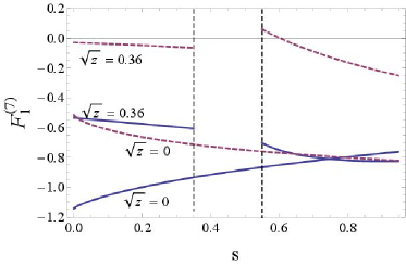
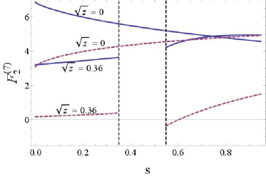
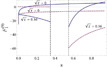
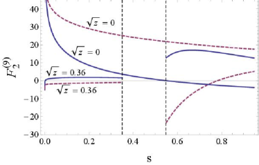
Figure 2: (Color online.) The real (solid lines) and imaginary (dotted lines) parts of the functions $F^{(7)}_{1,2}(s)$ (top two frames) and $F^{(9)}_{1,2}(s)$ (bottom two frames) at the scale $\mu=m_{b}$. For plotting the curves with $\sqrt{z}=0$, the exact analytic expressions Seidel (2004) were used. For non-zero values of $\sqrt{z}$, the analytic two-loop expressions obtained as double expansions in $\sqrt{z}$ and $s$ Asatrian et al. (2001); Asatryan et al. (2002) are used in plotting these functions in the region $s\leq 0.35$, whereas the expansions in $\sqrt{z}$ and $1-s$ Greub et al. (2008) are used in the range $0.55<s<1$. For these curves, we have fixed $\sqrt{z}=0.36$.

The renormalized $\alpha_{s}$-corrections $F^{(7)}_{1,2}(s)$ and $F^{(9)}_{1,2}(s)$ to the $b\to s\,\ell^{+}\ell^{-}$ matrix element originated by the ${\cal O}_{1}$- and ${\cal O}_{2}$-operators from the effective Hamiltonian (II) are known analytically both in the small-$q^{2}$ Asatrian et al. (2001); Asatryan et al. (2002) and large-$q^{2}$ Greub et al. (2008) domains of the lepton invariant mass squared as expansions in $\sqrt{z}=m_{c}/m_{b}$. Note that to obtain the invariant-mass spectrum and forward-backward asymmetry in the inclusive $B\to X_{s}\ell^{+}\ell^{-}$ decays the $F_{1,2,8}^{(7)}(s)$ and $F_{1,2,8}^{(9)}(s)$ functions were expressed in terms of master integrals and evaluated numerically Ghinculov et al. (2004). The functions $F_{1(2),u}^{(7)}(s)$ and $F_{1(2),u}^{(9)}(s)$ which are important in the $b\to d\,\ell^{+}\ell^{-}$ transitions were also calculated analytically first as an expansion in powers of $s$ Asatrian et al. (2004) and later exactly Seidel (2004) from which the later expressions are used by us as we are considering the $B\to\pi\ell^{+}\ell^{-}$ decay in the entire $q^{2}$-region.

The functions $F^{(7)}_{1,2}(s)$ (the top two frames) and $F^{(9)}_{1,2}(s)$ (the bottom two frames) are presented in Fig. 2 at the scale $\mu=m_{b}$ and $\sqrt{z}=0.36$. The real and imaginary parts of these functions are shown by the solid and dashed lines, respectively. The functions $F^{(7)}_{1,2}(s)$ and $F^{(9)}_{1,2}(s)$ at $\sqrt{z}=0$, which are obtained analytically in Ref. Seidel (2004), are also shown in Fig. 2. The vertical dashed lines specify the $s$-region where the expansions no longer hold. As the correct analytical functions in this region are not known for realistic value of $\sqrt{z}$, we have extrapolated the known analytic expressions from above and below (i. e., using expansions in $s$ and $1-s$) to a point in the intermediate region where the differential branching fraction has a minimal discontinuity. This allow us to get an approximate estimate of the perturbative part of the differential branching fraction in the gap between the $J/\psi$- and $\psi(2S)$-resonances.

In the analysis we also used the renormalized $\alpha_{s}$-corrections $F^{(7,9)}_{8}(s)$ from the ${\cal O}_{8}$-operator valid in the full kinematic $q^{2}$-domain ($0\leq s\leq 1$) Greub et al. (2008):

$$F^{(7)}_{8}(s) = \frac{4\pi^{2}}{27}\,\frac{2+s}{(1-s)^{4}}-\frac{16(2+s)}{3(1-s)^{4}}\arcsin^{2}\frac{\sqrt{s}}{2}$$

$$- \frac{8\sqrt{s(4-s)}}{9(1-s)^{3}}\left(9-5s+2s^{2}\right)\arcsin\frac{\sqrt{s}}{2}$$

$$- \frac{4(11-16s+8s^{2})}{9(1-s)^{2}}-\frac{8s\ln s}{9(1-s)}$$

$$- \frac{8i\pi}{9}-\frac{32}{9}\ln\frac{\mu}{m_{b}},$$

$$F^{(9)}_{8}(s) = -\frac{8\pi^{2}}{27}\,\frac{4-s}{(1-s)^{4}}+\frac{8(5-2s)}{9(1-s)^{2}}$$

$$+ \frac{16\sqrt{4-s}}{9\sqrt{s}\,(1-s)^{3}}\left(4+3s-s^{2}\right)\arcsin\frac{\sqrt{s}}{2}$$

$$+ \frac{32(4-s)}{3(1-s)^{4}}\arcsin^{2}\frac{\sqrt{s}}{2}+\frac{16\ln s}{9(1-s)},$$

where the $b$-quark mass $m_{b}$ is assumed to be the pole mass.

To perform the numerical analysis one needs to know the $B\to\pi$ transition form factors $f_{+}(q^{2})$, $f_{0}(q^{2})$ and $f_{T}(q^{2})$ in the entire kinematic range:

$$4m_{\ell}^{2}\leq q^{2}\leq\left(m_{B}-m_{\pi}\right)^{2}.$$ (30)

Their model-independent determination is the main aim of this paper, which is described in detail in subsequent sections.

III Form-Factor Parametrizations

Several parametrizations of the $B\to\pi$ transition form factors $f_{+}(q^{2})$, $f_{0}(q^{2})$ and $f_{T}(q^{2})$ have been proposed in the literature. The four parametrizations of $f_{+}(q^{2})$ discussed below have been used in the analysis of the semileptonic data on $B\to\pi\ell\nu_{\ell}$. All of them include at least one pole term at $q^{2}=m_{B^{*}}^{2}$, where $m_{B^{*}}=5.325$ GeV Beringer et al. (2012) is the vector $B^{*}$-meson mass. As far as this mass satisfies the condition $m_{B^{*}}<m_{B}+m_{\pi}$, i. e., it lies below the so-called continuum threshold, it should be included into the form factor as a separate pole. Other mesons and multi-particle states with the appropriate $J^{P}=1^{-}$ quantum number can be described either by one or several poles or by some other rapidly convergent function, both effectively counting the continuum. The tensor form factor $f_{T}(q^{2})$ shows a similar qualitative behavior and its model function obeys the same shape as the vector one. The case of the scalar form factor $f_{0}(q^{2})$ is different, as the first orbitally-excited scalar $B^{**}$-meson with $J^{P}=0^{+}$ has the mass squared above the continuum threshold $t_{0}=(m_{B}+m_{\pi})^{2}=29.36$ GeV² and, hence, it belongs to the continuum which makes $f_{0}(q^{2})$ regular at $q^{2}=m_{B^{*}}^{2}$, in contrast to $f_{+}(q^{2})$ and $f_{T}(q^{2})$.

III.1 The Becirevic-Kaidalov Parametrization

The form factor $f_{+}(q^{2})$ in the Becirevic-Kaidalov (BK) parametrization Becirevic and Kaidalov (2000) can be written as follows:

$$f_{+}(q^{2})=\frac{f_{+}(0)}{\left(1-\hat{q}_{*}^{2}\right)\left(1-\alpha_{\rm BK}\,\hat{q}_{*}^{2}\right)},$$ (31)

where $\hat{q}_{*}^{2}=q^{2}/m_{B^{*}}^{2}$. The fitted parameters are the form-factor normalization, $f_{+}(0)$, and $\alpha_{\rm BK}$ which defines the $f_{+}(q^{2})$ shape Becirevic and Kaidalov (2000). This parametrization is one of the simplest ones. The shape of the tensor form factor $f_{T}(q^{2})$ is the same (31) as it also has the pole at $q^{2}=m_{B^{*}}^{2}$ below the continuum threshold. The scalar form factor $f_{0}(q^{2})$ was also introduced in its simplest form Becirevic and Kaidalov (2000):

$$f_{0}(q^{2})=\frac{f_{+}(0)}{1-\hat{q}_{*}^{2}/\beta_{\rm BK}},$$ (32)

with the same normalization factor $f_{+}(0)$ but a different effective pole position determined by the free parameter $\beta_{\rm BK}$.

This form-factor parametrizations should be taken with caution, since the simple two-parameter shape is overly restrictive and has been argued to be inconsistent with the requirements from the Soft-Collinear Effective Theory (SCET) Becher and Hill (2006).

III.2 The Ball-Zwicky Parametrization

The Ball-Zwicky (BZ) parametrization for the vector form factor $f_{+}(q^{2})$ is a modified form of the BK parametrization, given as Ball and Zwicky (2005):

$$f_{+}(q^{2}) = \frac{f_{+}(0)}{1-\hat{q}_{*}^{2}}\left[1+\frac{r_{\rm BZ}\,\hat{q}_{*}^{2}}{1-\alpha_{\rm BZ}\,\hat{q}_{*}^{2}}\right]$$

$$= \frac{f_{+}(0)\left[1-\left(\alpha_{\rm BZ}-r_{\rm BZ}\right)\hat{q}_{*}^{2}\right]}{\left(1-\hat{q}_{*}^{2}\right)\left(1-\alpha_{\rm BZ}\hat{q}_{*}^{2}\right)},$$

where the fitted parameters are $f_{+}(0)$, $\alpha_{\rm BZ}$, and $r_{\rm BZ}$. $f_{+}(0)$ sets again the normalization of the form factor, while $\alpha_{\rm BZ}$ and $r_{\rm BZ}$ define the shape Ball and Zwicky (2005). In particular, for $\alpha_{\rm BZ}=r_{\rm BZ}$ one reproduces the BK parametrization (31). The same redefinition is also applied to the tensor form factor $f_{T}(q^{2})$. In a similar way the scalar form factor $f_{0}(q^{2})$ (32) can be modified by introducing its own second free parameter $r^{(0)}_{\rm BZ}$.

III.3 The Boyd-Grinstein-Lebed Parametrization

This parametrization was introduced for the form factors entering both the heavy-to-light Boyd et al. (1995a) and heavy-to-heavy Boyd et al. (1995b) transition matrix elements and used in the analysis of the semileptonic $B\to D^{(*)}\ell\nu_{\ell}$ Boyd et al. (1995b, 1996, 1997) and $B\to\pi\ell\nu_{\ell}$ Boyd et al. (1995a); Boyd and Savage (1997) decays. The basic idea is to find an appropriate function $z(q^{2},q_{0}^{2})$ in term of which the form factor can be written as a Taylor series with good convergence for all physical values of $q^{2}$ so that the form factor can be well described by the first few terms in the expansion. The generalization of this parametrization to additional form factors entering rare semileptonic $B\to h_{L}\,\ell^{+}\ell^{-}$, where $h_{L}$ is the pseudoscalar $K$- or the vector $\rho$- or $K^{*}$-mesons, and $B_{s}\to\phi\,\ell^{+}\ell^{-}$ decays, was undertaken in Bharucha et al. (2010). As this will be our default parametrization in our analysis, we discuss it at some length.

The following shape for the form factors $f_{i}(q^{2})$ with $i=+,0,T$ is suggested in the BGL parametrization Boyd et al. (1995a):

$$f_{i}(q^{2})=\frac{1}{P(q^{2})\phi_{i}(q^{2},q_{0}^{2})}\sum\limits_{k=0}^{k_{\rm max}}a_{k}(q_{0}^{2})\left[z(q^{2},q_{0}^{2})\right]^{k},$$ (34)

where the following form for the function $z(q^{2},q_{0}^{2})$ is used:

$$z(q^{2},q_{0}^{2})=\frac{\sqrt{m_{+}^{2}-q^{2}}-\sqrt{m_{+}^{2}-q_{0}^{2}}}{\sqrt{m_{+}^{2}-q^{2}}+\sqrt{m_{+}^{2}-q^{2}_{0}}},$$ (35)

with the pair-production threshold $m_{+}^{2}=(m_{B}+m_{\pi})^{2}$ and a free parameter $q_{0}^{2}$. The function $z(q^{2},q_{0}^{2})$ maps the entire range of $q^{2}$ onto the unit disc $|z|\leq 1$ in a way that the minimal physical value $z_{\rm min}=z(m_{-}^{2},q_{0}^{2})$ corresponds to the lowest hadronic recoil $q_{\rm max}^{2}=m_{-}^{2}=(m_{B}-m_{\pi})^{2}$, the maximal value $z_{\rm max}$ is reached at $q^{2}=0$, and $z(q^{2},q_{0}^{2})$ vanishes at $q^{2}=q_{0}^{2}$. In early studies of the form factors, the parameter $q_{0}^{2}$ was often taken to be $q_{0}^{2}=m_{-}^{2}$ Boyd et al. (1995a, b), so that $z_{\rm min}=0$. In this case, the maximal value $z_{\rm max}=0.52$ for the $B\to\pi\ell\nu_{\ell}$ decay is not small but enough to constrain the form factor $f_{+}(q^{2})$ Lellouch (1996); Boyd and Savage (1997). To decrease the value of $z_{\rm max}$, and improve the convergence of the Taylor series in Eq. (34), it was proposed to take a smaller (optimal) value of $q_{0}^{2}$ somewhere in the interval $0<q_{0}^{2}<m_{-}^{2}$ Boyd and Lebed (1997). In our analysis we make the choice $q^{2}_{0}=0.65m_{-}^{2}$ following del Amo Sanchez et al. (2011a), so that $-0.34<z(q^{2},q_{0}^{2})<0.22$ in the entire range $0<q^{2}<m_{-}^{2}$.

The proposed shape (34) for the form factor contains the so-called Blaschke factor $P(q^{2})$ which accounts for the hadronic resonances in the sub-threshold region $q^{2}<m_{+}^{2}$. For the semileptonic $B\to\pi\ell\nu_{\ell}$ decay, where $\ell$ is an electron or a muon, there is only the $B^{*}$-meson with the mass $m_{B^{*}}=5.325$ GeV satisfying the sub-threshold condition and producing the pole in the form factor at $q^{2}=m_{B^{*}}^{2}$. In this case, the Blaschke factor is simply $P(q^{2})=z(q^{2},m_{B^{*}}^{2})$ for $f_{+,T}(q^{2})$, and $P(q^{2})=1$ for $f_{0}(q^{2})$.

The coefficients $a_{k}$ ($k=0,1,\ldots,k_{\rm max}$) entering the Taylor series in Eq. (34) are the parameters, which are determined by the fits of the data. The outer function $\phi_{i}(q^{2},q_{0}^{2})$ is an arbitrary analytic function, whose choice only affects particular values of the coefficients $a_{k}$ and allows one to get a simple constraint from the dispersive bound Boyd and Savage (1997) :

$$\sum_{k=0}^{\infty}a_{k}^{2}\leq 1.$$ (36)

This restriction can be achieved with the following outer function Arnesen et al. (2005):

$$\phi_{i}(q^{2},q_{0}^{2}) = \sqrt{\frac{n_{I}}{K_{i}\chi_{f_{i}}^{(0)}}}\,\frac{(m_{+}^{2}-q^{2})^{(\alpha_{i}+1)/4}}{(m_{+}^{2}-q_{0}^{2})^{1/4}}$$

$$\times \left(\sqrt{m_{+}^{2}-q^{2}}+\sqrt{m_{+}^{2}-q_{0}^{2}}\right)$$

$$\times \left(\sqrt{m_{+}^{2}-q^{2}}+\sqrt{m_{+}^{2}-m_{-}^{2}}\right)^{\alpha_{i}/2}$$

$$\times \left(\sqrt{m_{+}^{2}-q^{2}}+m_{+}\right)^{-(3+\beta_{i})},$$

where $n_{I}=3/2$ is the isospin factor, while the values of $K_{i}$, $\alpha_{i}$ and $\beta_{i}$ are collected in Table 2.

Table 2: Parameters entering the outer functions $\phi_{i}(q^{2},q_{0}^{2})$ defined in Eq. (III.3) with $i=+,0,T$ in the $B\to\pi$ transition form factors.

$f_{i}$	$K_{i}$	$\alpha_{i}$	$\beta_{i}$	$\chi_{i}^{(0)}$
$f_{+}$	$48\pi$	3	2	$7.005\times 10^{-4}$ GeV-2
$f_{0}$	$16\pi/(m_{+}^{2}m_{-}^{2})$	1	1	$1.452\times 10^{-2}$
$f_{T}$	$48\pi m_{+}^{2}$	3	1	$1.811\times 10^{-3}$ GeV-2

The numerical quantities $\chi_{f_{i}}^{(0)}$ are obtained from the derivatives of the scalar functions entering the corresponding correlators calculated by the operator product expansion method Boyd and Lebed (1997); Boyd and Savage (1997); Bharucha et al. (2010). In the two-loop order at the scale $\mu_{b}$ they are as follows Bharucha et al. (2010):

$$\chi_{f_{+}}^{(0)} = \frac{3}{32\pi^{2}m_{b}^{2}}\left(1+\frac{C_{F}\alpha_{s}(\mu_{b})}{4\pi}\,\frac{25+4\pi^{2}}{6}\right)$$

$$- \frac{\langle\bar{q}q\rangle}{m_{b}^{5}}-\frac{\langle\alpha_{s}G^{2}\rangle}{12\pi m_{b}^{6}}+\frac{3\langle\bar{q}Gq\rangle}{m_{b}^{7}},$$

$$\chi_{f_{0}}^{(0)} = \frac{1}{8\pi^{2}}\left(1+\frac{C_{F}\alpha_{s}(\mu_{b})}{4\pi}\,\frac{3+4\pi^{2}}{6}\right)$$

$$+ \frac{\langle\bar{q}q\rangle}{m_{b}^{3}}+\frac{\langle\alpha_{s}G^{2}\rangle}{12\pi m_{b}^{4}}-\frac{3\langle\bar{q}Gq\rangle}{2m_{b}^{5}},$$

$$\chi_{f_{T}}^{(0)} = \frac{1}{4\pi^{2}m_{b}^{2}}\left(1+\frac{C_{F}\alpha_{s}(\mu_{b})}{4\pi}\left[\frac{10+2\pi^{2}}{3}+8\ln\frac{m_{b}}{\mu_{b}}\right]\right)$$ (40)

$$- \frac{\langle\bar{q}q\rangle}{m_{b}^{5}}-\frac{\langle\alpha_{s}G^{2}\rangle}{24\pi m_{b}^{6}}+\frac{7\langle\bar{q}Gq\rangle}{2m_{b}^{7}},$$

where $C_{F}=4/3$, and $m_{b}$ is the mass of the $b$-quark in the loops which is identified with the $\overline{\rm MS}$ $b$-quark mass $\bar{m}_{b}(\bar{m}_{b})=4.18$ GeV Beringer et al. (2012). For the evaluation of $\chi_{f_{i}}^{(0)}$ it is enough to use the central values of the input parameters to get the overall numerical normalization factor for the form factors and the existing uncertainties in $\chi_{f_{i}}^{(0)}$ are of not much consequence. The following input values are used: $\alpha_{s}(M_{Z})=0.1184\pm 0.0007$ Beringer et al. (2012), $\langle\bar{q}q\rangle(1~{}{\rm GeV})=-(1.65\pm 0.15)\times 10^{-2}$ GeV³, $\langle\bar{q}Gq\rangle=\langle\bar{q}g_{s}\sigma^{\mu\nu}G_{\mu\nu}^{A}T^{A}q\rangle=m_{0}^{2}\langle\bar{q}q\rangle$, $m_{0}^{2}(1~{}{\rm GeV})=(0.8\pm 0.2)$ GeV², and $\langle(\alpha_{s}/\pi)\,G^{2}\rangle=(0.005\pm 0.004)$ GeV⁴ from Ref. Ioffe (2006). While the mixed quark-gluon $\langle\bar{q}Gq\rangle$ and the two-gluon $\langle(\alpha_{s}/\pi)\,G^{2}\rangle$ condensates are practically scale-independent quantities Ioffe (2006), the strong coupling and the quark condensate have to be evolved to the scale of the $b$-quark mass where they have the values $\alpha_{s}(\bar{m}_{b})=0.227$ to the two-loop accuracy and $\langle\bar{q}q\rangle(\bar{m}_{b})=-0.023$ GeV³. Numerical values of $\chi_{f_{i}}^{(0)}$ are presented in Table 2. They agree well (up to 5%) with the ones presented in Table 2 of Bharucha et al. (2010), despite differences in the input parameters. Note that the BaBar Collaboration del Amo Sanchez et al. (2011a) used approximately the same value $\chi_{f_{+}}^{(0)}=6.889\times 10^{-4}$ GeV^-2 in the analysis of the $B^{0}\to\pi^{+}\ell^{-}\nu_{\ell}$ decays.

Having relatively small values of $z(q^{2},q_{0}^{2})$ in the physical region of $q^{2}$, the shape of the form factor can be well approximated by the truncated series at $k_{\rm max}=2$ or $3$ Boyd et al. (1996).

III.4 The Bourrely-Caprini-Lellouch Parametrization

The problems with the from-factor asymptotic behavior at $|q^{2}|\to\infty$ and truncation of the Taylor series found in the BGL-parametrization Becher and Hill (2006); Bourrely et al. (2009) were solved by the introduction of another representation of the series expansion (called the Simplified Series Expansion — SSE Bharucha et al. (2010)). The shape suggested for the vector $f_{+}(q^{2})$ form factor Bourrely et al. (2009) was extended to the other two, scalar $f_{0}(q^{2})$ and tensor $f_{T}(q^{2})$, form factors Bharucha et al. (2010):

$$f_{+}(q^{2}) = \frac{1}{1-\hat{q}_{*}^{2}}\sum\limits_{k=0}^{k_{\rm max}}b^{(+)}_{k}(q_{0}^{2})\left[z(q^{2},q_{0}^{2})\right]^{k},$$ (41)

$$f_{0}(q^{2}) = \frac{m_{B}^{2}}{m_{B}^{2}-m_{\pi}^{2}}\sum\limits_{k=0}^{k_{\rm max}}b^{(0)}_{k}(q_{0}^{2})\left[z(q^{2},q_{0}^{2})\right]^{k},$$ (42)

$$f_{T}(q^{2}) = \frac{m_{B}+m_{\pi}}{m_{B}\left(1-\hat{q}_{*}^{2}\right)}\sum\limits_{k=0}^{k_{\rm max}}b^{(T)}_{k}(q_{0}^{2})\left[z(q^{2},q_{0}^{2})\right]^{k},$$ (43)

where $\hat{q}_{*}^{2}=q^{2}/m_{B^{*}}^{2}$ and the function $z(q^{2},q_{0}^{2})$ is defined in Eq. (35). In this expansion the shape of the form factor is determined by the values of $b_{k}$, with truncation at $k_{\rm max}=2$ or $3$. The value of the free parameter $q_{0}^{2}$ is proposed to be the so-called optimal one $q_{0}^{2}=q_{\rm opt}^{2}=\left(m_{B}+m_{\pi}\right)\left(\sqrt{m_{B}}-\sqrt{m_{\pi}}\right)^{2}$ Bourrely et al. (2009), which is obtained as the solution of the equation $z(0,q_{0}^{2})=-z(m_{-}^{2},q_{0}^{2})$ (the latter condition means that the physical range $0<q^{2}\leq m_{-}^{2}$ is projected onto a symmetric interval on the real axis in the complex $z$-plane). The prefactors $1/(1-\hat{q}_{*}^{2})$ in $f_{+}(q^{2})$ and $f_{T}(q^{2})$ allow one to get the right asymptotic behavior $\sim 1/q^{2}$ predicted by the perturbative QCD. In Ref. Becher and Hill (2006); Bourrely et al. (2009) an additional restriction on the series coefficients was discussed. In particular, in the case of $f_{+}(q^{2})$ at $q^{2}\sim m_{+}^{2}$, the threshold behavior of the form factor results in a constraint on its derivative, $df_{+}/dz|_{z=-1}=0$ Bourrely et al. (2009), which allows one to eliminate the last term in the truncated expansion as follows:

$$b^{(+)}_{k_{\rm max}}(q_{0}^{2})=-\frac{(-1)^{k_{\rm max}}}{k_{\rm max}}\sum_{k=0}^{k_{\rm max}-1}(-1)^{k}\,k\,b^{(+)}_{k}(q_{0}^{2}).$$ (44)

In the case of $f_{0}(q^{2})$ the threshold behavior is different and a similar relation is not applied. A detailed analysis of the additional constraints based on the threshold behavior of the tensor $f_{T}(q^{2})$ form factor in the $B\to\pi$ transition has not yet been performed. This behavior, however, is not expected to be very different from the one found for the vector $f_{+}(q^{2})$ form factor. So, one may as well put the condition on the derivative $df_{T}/dz|_{z=-1}=0$ in this case, which allows to eliminate the last term in the truncated expansion for $f_{T}(q^{2})$. This was used in the analysis applied for fitting the tensor $B\to K$ transition form factor by the HPQCD Collaboration Bouchard et al. (2013b).

IV Extraction of the $f_{+}(q^{2})$ Form-Factor Shape

IV.1 The $B^{0}\to\pi^{-}\ell^{+}\nu_{\ell}$ Branching Fraction

The charged-current Lagrangian inducing the $b\to u$ transition in the SM is:

$${\cal L}_{W}(x)=-\frac{g}{2\sqrt{2}}\,V_{ub}\left[\bar{u}(x)\gamma_{\mu}\left(1-\gamma_{5}\right)b(x)\right]W^{\mu}(x)+\mathrm{h.\ c.},$$ (45)

where $g$ is the $SU(2)_{L}$ coupling, $V_{ub}$ is the element of the CKM matrix, $u(x)$ and $b(x)$ are the $u$- and $b$-quark fields, and $W(x)$ is the $W$-boson field. Feynman diagram for the $B^{0}\to\pi^{-}\ell^{+}\nu_{\ell}$ decay is shown in Fig. 3 and the one for the $B^{+}\to\pi^{0}\ell^{+}\nu_{\ell}$ decay differs by the exchange of the spectator-quark flavor ($d\to u$) only.

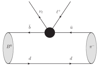
Figure 3: Feynman diagram for the $B^{0}\to\pi^{-}\ell^{+}\nu_{\ell}$ decay.

The $B\to\pi$ transition matrix element entering the $B$-meson decay $B\to\pi\ell\nu_{\ell}$ can be parametrized in terms of two form factors $f_{+}(q^{2})$ and $f_{0}(q^{2})$ as follows Neubert (1994); Burdman et al. (1994):

$$\langle\pi(p_{\pi})|\bar{u}\gamma^{\mu}b|B(p_{B})\rangle = f_{+}(q^{2})\left[p_{B}^{\mu}+p_{\pi}^{\mu}-\frac{m_{B}^{2}-m_{\pi}^{2}}{q^{2}}\,q^{\mu}\right]$$ (46)

$$+ f_{0}(q^{2})\,\frac{m_{B}^{2}-m_{\pi}^{2}}{q^{2}}\,q^{\mu}.$$

Here, $p_{B}$ ($m_{B}$) and $p_{\pi}$ ($m_{\pi}$) are the four-momenta (masses) of the $B$- and $\pi$-mesons, respectively. In the isospin-symmetry limit, the form factors in the charged-current matrix element (46) are exactly the same as the ones in Eq. (10) in the FCNC process $B\to\pi\,\ell^{+}\ell^{-}$.

Measurements of the $B^{0}\to\pi^{-}\ell^{+}\nu_{\ell}$ and $B^{+}\to\pi^{0}\ell^{+}\nu_{\ell}$ decays, where $\ell=e,\,\mu$, allow to extract both the CKM matrix element $|V_{ub}|$ and the shape of the $f_{+}(q^{2})$ form factor. The differential branching fractions of the above processes can be written in the form Beringer et al. (2012):

$$\frac{d\Gamma(B\to\pi\ell^{+}\nu_{\ell})}{dq^{2}}=C_{P}\,\frac{G_{F}^{2}|V_{ub}|^{2}}{192\pi^{3}m_{B}^{3}}\,\lambda^{3/2}(q^{2})f_{+}^{2}(q^{2}),$$ (47)

where $G_{F}$ is the Fermi constant, $C_{P}$ is the isospin factor with $C_{P}=1$ for the $\pi^{+}$-meson and $C_{P}=1/2$ for the $\pi^{0}$-meson, $\lambda(q^{2})$ is the standard three-body kinematic factor (13), $q^{\mu}=p_{\ell}^{\mu}+p_{\nu}^{\mu}$ is the total four-momentum transfer, bounded by $m_{\ell}^{2}\leq q^{2}\leq(m_{B}-m_{\pi})^{2}$, and $p_{\ell}^{\mu}$ and $p_{\nu}^{\mu}$ are the four-momenta of the charged lepton and the neutrino, respectively. In general, the $B\to\pi$ transition matrix element (46) depends on two form factors. In practice, however, only $f_{+}(q^{2})$ is measurable in the $B\to\pi\ell\nu_{\ell}$ decays with $\ell=e,\mu$, since the contribution of the scalar form factor $f_{0}(q^{2})$ to the decay rate is suppressed by the mass ratio of the charged lepton to the $B$-meson Burdman et al. (1994).

The values of $G_{F}$, $m_{B}$, and $m_{\pi}$ are known with high accuracy Beringer et al. (2012), while the experimentally derived value of $|V_{ub}|$ depends somewhat on the extraction method and $B$-meson decays considered. This is discussed at great length in the Particle Data Group (PDG) reviews Beringer et al. (2012). The value quoted from the analysis of the exclusive $B\to\pi\ell\nu_{\ell}$ decay is listed there as $|V_{ub}|=(3.23\pm 0.31)\times 10^{-3}$. On the other hand, assuming the SM, the CKM unitarity fits yield a value of $|V_{ub}|$ which is consistent with the previous value, but is about a factor 2 more precise Beringer et al. (2012): $|V_{ub}|=(3.51^{+0.15}_{-0.14})\times 10^{-3}$, which we use as our default value in the numerical estimates.

The partial branching fractions for the $B^{0}\to\pi^{-}\ell^{+}\nu_{\ell}$ decays has been measured by the CLEO, BaBar and Belle collaborations, and for the $B^{+}\to\pi^{0}\ell^{+}\nu_{\ell}$ decays by the Belle Collaboration. Below we give the total branching fraction of the $B^{0}\to\pi^{-}\ell^{+}\nu_{\ell}$ decay taking into account the recent data from the BaBar and Belle collaborations del Amo Sanchez et al. (2011b); Lees et al. (2012); Ha et al. (2011); Sibidanov et al. (2013):

$$\begin{split}&{\cal B}(B^{0}\to\pi^{-}\ell^{+}\nu_{\ell})\\ &=\left\{\begin{array}[]{rl}\!(1.42\pm 0.05_{\rm stat}\pm 0.07_{\rm syst})\times 10^{-4}&[\mbox{BaBar, 2011}]~{},\\ \!(1.45\pm 0.04_{\rm stat}\pm 0.06_{\rm syst})\times 10^{-4}&[\mbox{BaBar, 2012}]~{},\\ \!(1.49\pm 0.04_{\rm stat}\pm 0.07_{\rm syst})\times 10^{-4}&[\mbox{Belle, 2011}]~{},\\ \!(1.49\pm 0.09_{\rm stat}\pm 0.07_{\rm syst})\times 10^{-4}&[\mbox{Belle, 2013}]~{}.\end{array}\right.\end{split}$$ (48)

All these measurements are in excellent agreement with each other, and with the one for the $B^{+}\to\pi^{0}\ell^{+}\nu_{\ell}$ decay reported by the Belle Collaboration Sibidanov et al. (2013):

$${\cal B}(B^{+}\to\pi^{0}\ell^{+}\nu_{\ell})=(0.80\pm 0.08_{\rm stat}\pm 0.04_{\rm syst})\times 10^{-4}.$$ (49)

Both the collaborations have presented differential distributions in $q^{2}$ relevant for the extraction of $f_{+}(q^{2})$ from data del Amo Sanchez et al. (2011b); Lees et al. (2012); Ha et al. (2011); Sibidanov et al. (2013). We show them in the next subsection, where also our fitting procedure is presented.

IV.2 Fitting Procedure

In this subsection the extraction of the $f_{+}(q^{2})$ form-factor shape from the dilepton invariant-mass spectra in the $B^{0}\to\pi^{-}\ell^{+}\nu_{\ell}$ and $B^{+}\to\pi^{0}\ell^{+}\nu_{\ell}$ decays measured by the BaBar del Amo Sanchez et al. (2011b); Lees et al. (2012) and Belle Ha et al. (2011); Sibidanov et al. (2013) collaborations is explained. All four $f_{+}(q^{2})$ form-factor parametrizations from Sec. III are examined to test their consistency with the experiment in terms of the best-fit values resulting from the $\chi^{2}$-distribution function Beringer et al. (2012).

The fitted form factor is presented as a function of $q^{2}$ which contains a set of $k$ unknown parameters $\alpha_{1},\ldots,\alpha_{k}$:

$$f_{+}(q^{2})=f(q^{2};\alpha_{1},\ldots,\alpha_{k}).$$ (50)

Given the experimental values $y_{i}$ of the partial branching fractions $\Delta{\cal B}(q^{2})/\Delta q^{2}$ in bins of $q^{2}$, with their uncertainties $\sigma_{i}$, the $\chi^{2}$-distribution function is defined as follows Beringer et al. (2012):

$$\chi^{2}=\sum\limits_{i=1}^{N}\frac{\left[y_{i}-F(x_{i};\alpha_{1},\ldots,\alpha_{k})\right]^{2}}{\sigma_{i}^{2}},$$ (51)

where $N$ is the number of experimental points and $F(x_{i};\alpha_{1},\ldots,\alpha_{k})$ denotes the theoretical estimates of the partial branching fractions $\Delta{\cal B}(q^{2})/\Delta q^{2}$ for the given parametrization:

$$F(x_{i};\alpha_{1},\ldots,\alpha_{k})=\int\limits_{x_{i}-a_{i}/2}^{x_{i}+a_{i}/2}\!\frac{d{\cal B}(q^{2})}{dq^{2}}\,dq^{2},$$ (52)

with $x_{i}$ and $a_{i}$ being the center and the width of the $i$th bin. The standard minimization procedure of the $\chi^{2}$-function (minimum of this function is denoted as $\chi^{2}_{\rm min}$) allows us to extract the values of fitted parameters $\alpha_{1,{\rm min}},\ldots,\alpha_{k,{\rm min}}$, which are considered to be their best-fit values. The results obtained by using the four form-factor parametrizations for different sets of experimental data obtained by the BaBar del Amo Sanchez et al. (2011b); Lees et al. (2012) and Belle Ha et al. (2011); Sibidanov et al. (2013) collaborations are presented in Figs. 4 and 5, respectively, and the numerical values for $\chi_{\rm min}^{2}$/ndf, where ndf is the number of degrees of freedom, and the corresponding $p$-values are presented in Table 3. In this analysis we have assumed that the experimental points are all uncorrelated.

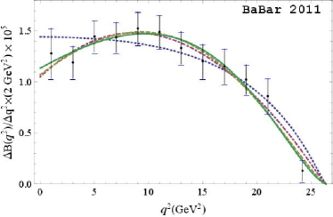
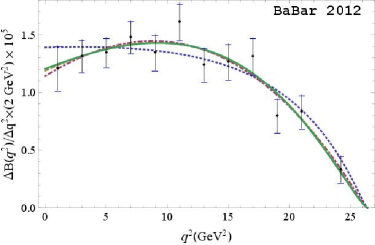
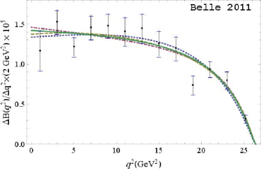
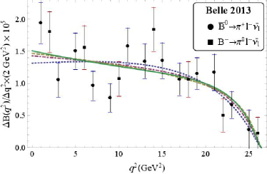
Figure 4: (Color online.) Partial $\Delta{\cal B}(q^{2})/\Delta q^{2}$ spectra for the $B^{0}\to\pi^{-}\ell^{+}\nu_{\ell}$ and $B^{+}\to\pi^{0}\ell^{+}\nu_{\ell}$ decays, where $\ell=e,\,\mu$. The data points (black dots and squares) are placed in the middle of each bin. The error bars (blue) include the total experimental uncertainties. The curves show the results of the fit to the data for the four form-factor parametrizations discussed in the text: BK (31) (thick dotted blue line), BZ (III.2) (thick dashed purple line), BGL (34) with $k_{\rm max}=2$ (thick dot-dashed yellow line), and BCL (41) with $k_{\rm max}=2$ (thick solid green line). The upper-left and upper-right plots correspond to the BaBar 2011 del Amo Sanchez et al. (2011b) and 2012 Lees et al. (2012) data sets, while the lower-left and lower-right plots are plotted based on the Belle 2011 Ha et al. (2011) and 2013 Sibidanov et al. (2013) data sets.

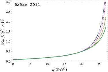
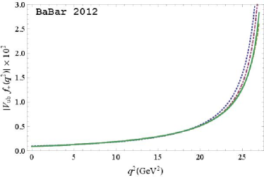
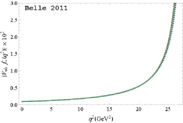
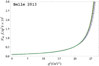
Figure 5: (Color online.) The $f_{+}(q^{2})$ form-factor shapes in the decay $B\to\pi\ell\nu_{\ell}$ multiplied by the CKM matrix element $|V_{ub}|$ following from the BaBar del Amo Sanchez et al. (2011b); Lees et al. (2012) and Belle Ha et al. (2011); Sibidanov et al. (2013) data. The curves show the results of the fit to these data: BK (31) (thick dotted blue line), BZ (III.2) (thick dashed purple line), BGL (34) with $k_{\rm max}=2$ (thick dot-dashed yellow line), and BCL (41) with $k_{\rm max}=2$ (thick solid green line) parametrizations.

Table 3: Summary of the $\chi_{\rm min}^{2}$/ndf values, where ndf is the number of degrees of freedom, (corresponding $p$-values) for different sets of experimental data (rows) and four form-factor parametrizations discussed in the text (columns).

	BK Becirevic and Kaidalov (2000)	BZ Ball and Zwicky (2005)	BGL Boyd et al. (1996)	BCL Bourrely et al. (2009)
BaBar 2011 del Amo Sanchez et al. (2011b)	9.93/10 (45%)	4.80/9 (85%)	4.12/9 (90%)	3.75/9 (93%)
BaBar 2012 Lees et al. (2012)	8.68/10 (56%)	5.50/9 (79%)	5.65/9 (77%)	5.73/9 (77%)
Belle 2011 Ha et al. (2011)	15.86/11 (15%)	14.55/10 (15%)	12.97/10 (23%)	14.44/10 (15%)
Belle 2013 Sibidanov et al. (2013)	24.41/18 (14%)	23.55/17 (13%)	24.16/17 (12%)	23.26/17 (14%)
BaBar & Belle	44.99/43 (39%)	44.91/42 (35%)	44.56/42 (36%)	44.77/42 (36%)

From Table 3 it follows that the smallest value for $\chi_{\rm min}^{2}$/ndf corresponds to the simplest Becirevic-Kaidalov parametrization. From the rest of the specified parametrizations, the Boyd-Grinstein-Lebed one has the smallest $\chi_{\rm min}^{2}$/ndf value and we will use it for all the form factors entering the $B\to\pi\ell^{+}\ell^{-}$ decay.

The combined analysis of the BaBar and Belle data yields the following set of fitted parameters entering the $f_{+}(q^{2})$ form factor expansion in the BGL parametrization, truncated at $k_{\rm max}=2$:

$$a_{0} = \hphantom{-}0.0209\pm 0.0004,$$

$$a_{1} = -0.0306\pm 0.0031,$$ (53)

$$a_{2} = -0.0473\pm 0.0189.$$

The extracted numerical values depend on the CKM matrix element $|V_{ub}|$ and correspond to the PDG value Beringer et al. (2012): $|V_{ub}|=(3.51^{+0.15}_{-0.14})\times 10^{-3}$. The errors specified in the coefficients (53) are the square roots of the covariance matrix $U_{ij}$ for the BGL form-factor coefficients which can be derived from the $\chi^{2}$-function (51) as follows Beringer et al. (2012):

$$\left(U^{-1}\right)_{ij}=\frac{1}{2}\left.\frac{\partial^{2}\chi^{2}}{\partial\alpha_{i}\partial\alpha_{j}}\right|_{\alpha_{k}=\hat{\alpha}_{k}},$$ (54)

where $\hat{\alpha}_{k}$ are the best-fit values of the fitting parameters. The function $F(x_{i};\alpha_{1},\ldots,\alpha_{k})$ in the BGL form factor depends linearly on the unknown parameters, which simplifies the analysis. The corresponding correlation matrix $r_{ij}$ is connected with the covariance matrix by the relation $r_{ij}=U_{ij}/(\sigma_{i}\,\sigma_{j})$, where $\sigma_{i}^{2}$ is the variance of $\alpha_{i}$. For the BGL form factor with the truncation at $k_{\rm max}=2$, the following $(3\times 3)$ correlation matrix was obtained:

$$r_{ij}=\left(\begin{array}[]{ccc}1&-0.26&-0.43\\ -0.26&1&-0.68\\ -0.43&-0.68&1\end{array}\right).$$ (55)

One can see the sizable correlation of the third coefficient $a_{2}$ in the $z$-expansion with the other two $a_{0}$ and $a_{1}$. This is shown in Fig. 6. The relative error on the coefficient $a_{2}$ is approximately 40% as can also be seen in Eq. (53).

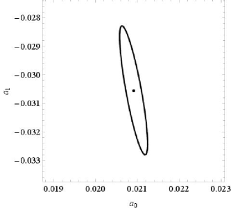
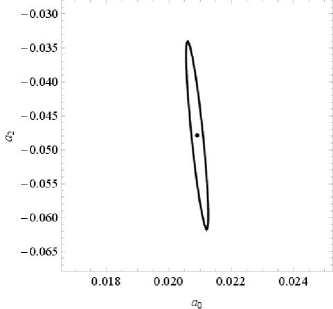
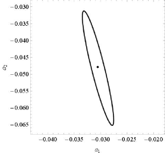
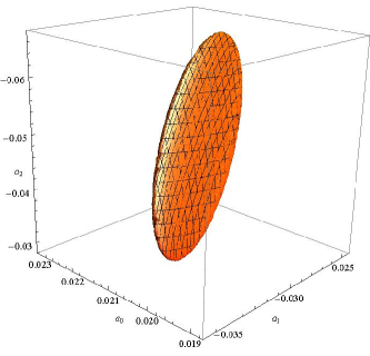
Figure 6: (Color online.) The two-dimensional correlations among the fitted parameters $a_{0}$, $a_{1}$ and $a_{2}$ entering the BGL-parametrization of the form factor $f_{+}(q^{2})$: $a_{0}-a_{1}$ (upper-left plot), $a_{0}-a_{2}$ (upper-right plot) and $a_{1}-a_{2}$ (lower-left plot). The three-dimensional correlation among all three fitted parameters is shown in the lower-right plot.

The results from the combined analysis of the BaBar Lees et al. (2012) and Belle Ha et al. (2011); Sibidanov et al. (2013) data sets are shown in Fig. 7 (upper plot).

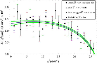
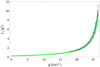
Figure 7: (Color online.) Partial $\Delta{\cal B}(q^{2})/\Delta q^{2}$ spectra for the decays $B^{0}\to\pi^{-}\ell^{+}\nu_{\ell}$ and $B^{+}\to\pi^{0}\ell^{+}\nu_{\ell}$ are presented on the upper plot. The $f_{+}(q^{2})$ form factor is shown on the lower plot. The BGL parametrization is adopted as the preferred choice. Results are obtained by combining the experimental data by the BaBar Lees et al. (2012) and Belle Ha et al. (2011); Sibidanov et al. (2013) collaborations and, in addition, the value $|V_{ub}|=(3.51^{+0.15}_{-0.14})\times 10^{-3}$ Beringer et al. (2012) is used to extract explicitly the form-factor shape. The existing Lattice-QCD data Dalgic et al. (2006) on the form factor are presented as the vertical bars on the lower plot.

Following the numerical analysis presented above, the resulting shape of the $f_{+}(q^{2})$ form factor is presented on the lower plot in Fig. 7, using the BGL parametrization and the PDG value $|V_{ub}|=(3.51^{+0.15}_{-0.14})\times 10^{-3}$ Beringer et al. (2012). The existing Lattice-QCD results Dalgic et al. (2006) on the $f_{+}(q^{2})$ form factor are presented as vertical bars on the lower plot in Fig. 7, which are in good agreement with our estimate of the same in the overlapping $q^{2}$-region (within the uncertainties of the lattice data, as indicated).

V Determination of $f_{0}(q^{2})$ and $f_{T}(q^{2})$ Shapes

As pointed out earlier, the form factor $f_{0}(q^{2})$ is not required for either the charged-current decay $B\to\pi\ell\nu_{\ell}$ or the FCNC semileptonic $B\to\pi\ell^{+}\ell^{-}$ decay with $\ell=e,\mu$, as its contribution to the branching fraction is suppressed by the smallness of the lepton mass squared. However, for the sake of completeness involving the semileptonic processes with $\ell^{\pm}=\tau^{\pm}$, we also work out the $f_{0}(q^{2})$ form factor. The information on the form factors $f_{+}(q^{2})$ and $f_{0}(q^{2})$ for the $B\to\pi$ and $B\to K$ transitions is available, though the lattice results on the $B\to\pi$ form factor $f_{T}(q^{2})$ are still scant. For our analysis, we use an Ansatz for the $SU(3)_{F}$-symmetry breaking to obtain the shape of $f^{B\pi}_{T}(q^{2})$ from the corresponding $B\to K$ form factor $f^{BK}_{T}(q^{2})$. We show subsequently that our Ansatz, which assumes that the $SU(3)_{F}$-symmetry breaking in $f_{T}(q^{2})$ is an average of the corresponding symmetry-breaking effects in the form factors $f_{+}(q^{2})$ and $f_{0}(q^{2})$, yields an $f^{B\pi}_{T}(q^{2})$, which is in good agreement with the preliminary results on this form factor, obtained from lattice in the low-recoil region.

V.1 The $f_{0}(q^{2})$ Form Factor

The parameters in $f_{0}(q^{2})$ can be obtained from the existing results of the $B\to\pi$ transition form factor calculated by the HPQCD Collaboration Dalgic et al. (2006). In addition we use the exact relation between $f_{+}(q^{2})$ and $f_{0}(q^{2})$ at $q^{2}=0$:

$$f_{+}(0)=f_{0}(0),$$ (56)

which follows from the requirement of the finiteness of the $B\to\pi$ transition matrix element (10) at this point. To fix $f_{0}(0)$, we use the reference point $f_{+}(0)=0.261\pm 0.014$, extracted by us from the experimental data. The form-factor parametrization we use for $f_{0}(q^{2})$ follows our default choice from the analysis of $f_{+}(q^{2})$ — the BGL expansion in $z(q^{2},q_{0}^{2})$ truncated at $k_{\rm max}=2$. The set of the fitted parameters entering $f_{0}(q^{2})$ is as follows:

$$a_{0} = \hphantom{-}0.0201\pm 0.0007,$$

$$a_{1} = -0.0394\pm 0.0096,$$ (57)

$$a_{2} = -0.0355\pm 0.0556,$$

and the correlation matrix ($i,j=1,2,3$) is:

$$r_{ij}=\left(\begin{array}[]{ccc}1&0.72&-0.82\\ 0.72&1&-0.96\\ -0.82&-0.96&1\end{array}\right).$$ (58)

One sees strong correlations among all the fitted parameters, which can be well approximated as linear. The resulting shape is shown in Fig. 8. The solid (green) lines specify the from-factor uncertainty which grows with increasing $q^{2}$. This trend is reflected also in the lattice data Dalgic et al. (2006) (shown by the vertical bars in Fig. 8).

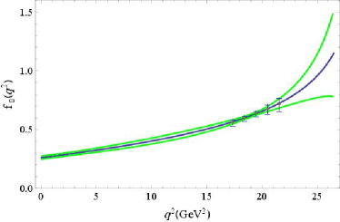
Figure 8: (Color online.) The scalar $B\to\pi$ transition form factor $f_{0}(q^{2})$ in the entire kinematic region using the BGL parametrization. The solid green lines show the uncertainty in the form factor. The vertical bars are the Lattice-QCD data Dalgic et al. (2006) used for fixing the form-factor shape.

V.2 The $f_{T}(q^{2})$ Form Factor

As already mentioned, there is at present only scant information from the lattice on the $B\to\pi$ tensor form factor $f_{T}^{B\pi}(q^{2})$. So, one needs to find a reliable method to extract it from the existing model-independent data. We use an $SU(3)_{F}$-symmetry breaking Ansatz involving both the $B\to K$ and $B\to\pi$ transition form factors. We recall that all three $B\to K$ transition form factors $f_{+}^{BK}(q^{2})$, $f_{0}^{BK}(q^{2})$ and $f_{T}^{BK}(q^{2})$ have been calculated recently by the HPQCD Collaboration Bouchard et al. (2013b, a) and the two $B\to\pi$ transition form factors $f_{+}^{B\pi}(q^{2})$ and $f_{0}^{B\pi}(q^{2})$ are also known Dalgic et al. (2006). Of course, lattice results are available only in the small-recoil limit. With this at hand, we first estimate the $SU(3)_{F}$-symmetry-breaking corrections in the already known vector and scalar form factors and use these corrections to estimate the $B\to\pi$ tensor form factor $f_{T}^{B\pi}(q^{2})$ from the corresponding $B\to K$ transition form factor $f_{T}^{BK}(q^{2})$. We introduce the following measures of the $SU(3)_{F}$-symmetry breaking corrections in the transition form factors:

$$R_{i}(q^{2})=\frac{f_{i}^{BK}(q^{2})}{f_{i}^{B\pi}(q^{2})}-1,$$ (59)

where $i=+,\,0,\,T$. The curves for the $SU(3)_{F}$-symmetry breaking functions $R_{+}(q^{2})$ and $R_{0}(q^{2})$, calculated for the central values of the form factors from the lattice for the small-recoil region, are presented in the upper plot in Fig. 9. As expected, breaking effects of order 10% are seen in both the ratios. We expect that the $SU(3)_{F}$-symmetry breaking effect in the third ratio, $R_{T}(q^{2})$, is of the same order. For the sake of definiteness, we assume that the ratio $R_{T}(q^{2})$ of the tensor form factors is the average of the other two: $R_{+}(q^{2})$ and $R_{0}(q^{2})$,

$$R_{T}(q^{2})=\frac{1}{2}\left[R_{+}(q^{2})+R_{0}(q^{2})\right].$$ (60)

We estimate the accuracy of this relation in the low-$q^{2}$ region, where the methods based on HQS (and its leading-order breakings) can be gainfully used to quantify it (see Sec. VI.3 for details). We expect that this relation holds to a good extent in the remaining large-$q^{2}$ region, and estimate the associated uncertainty to be about 5%. The corresponding function $R_{T}(q^{2})$ is presented in the upper plot in Fig. 9 as the central curve. Explicit values of this function in the small-recoil region are presented in Table 4. The errors reflect the uncertainties of the lattice calculations and we assume that the errors in the $B\to\pi$ and $B\to K$ transition form factors are uncorrelated.

The values of the $f_{T}^{B\pi}(q^{2})$ form factor are then obtained by rescaling them from the known values of the $f_{T}^{BK}(q^{2})$ form factor Bouchard et al. (2013b) by utilizing the relation:

$$f_{T}^{B\pi}(q^{2})=\frac{f_{T}^{BK}(q^{2})}{1+R_{T}(q^{2})}~{}.$$ (61)

They are presented in Table 4. The variance of $f_{T}^{B\pi}(q^{2})$ is calculated by adding the errors of $f_{T}^{BK}(q^{2})$ and $R_{T}(q^{2})$ in quadrature. The normalization at $q^{2}=0$: $f_{T}^{B\pi}(0)=0.231\pm 0.013$, which results from the value $f_{+}^{B\pi}(0)=0.261\pm 0.014$, extracted by us from the experimental data on the $B\to\pi\ell\nu_{\ell}$ decays, and the heavy-quark symmetry relation between the form factors in the large-recoil limit of the $\pi$-meson Charles et al. (1999); Beneke and Feldmann (2001): $f^{B\pi}_{T}(0)=\left(1+m_{\pi}/m_{B}\right)f^{B\pi}_{+}(0)$. With all this at hand, we have a fairly constrained model for the $f_{T}^{B\pi}(q^{2})$ form factor.

Table 4: Values of the tensor form factor $f_{T}^{B\pi}(q^{2})$ at the indicated values of $q^{2}$ obtained from the existing Lattice-QCD data on the $f_{T}^{BK}(q^{2})$ transition form factor Bouchard et al. (2013b) and the $SU(3)_{F}$-symmetry breaking function $R_{T}(q^{2})$ defined in Eqs. (59) and (60). The variance of $f_{T}^{B\pi}(q^{2})$ is calculated by adding the errors of $f_{T}^{BK}(q^{2})$ and $R_{T}(q^{2})$ in quadrature.

$q^{2}$, GeV2	18.4	19.1	19.8	20.6
$f_{T}^{BK}(q^{2})$	$1.197\pm 0.047$	$1.307\pm 0.051$	$1.434\pm 0.057$	$1.608\pm 0.069$
$R_{T}(q^{2})$	$0.080\pm 0.021$	$0.076\pm 0.021$	$0.073\pm 0.023$	$0.071\pm 0.023$
$f_{T}^{B\pi}(q^{2})$	$1.108\pm 0.126$	$1.215\pm 0.115$	$1.337\pm 0.117$	$1.503\pm 0.123$
$q^{2}$, GeV2	21.3	22.1	22.8	23.5
$f_{T}^{BK}(q^{2})$	$1.793\pm 0.082$	$2.054\pm 0.106$	$2.342\pm 0.135$	$2.713\pm 0.176$
$R_{T}(q^{2})$	$0.070\pm 0.037$	$0.072\pm 0.050$	$0.076\pm 0.067$	$0.083\pm 0.090$
$f_{T}^{B\pi}(q^{2})$	$1.675\pm 0.144$	$1.916\pm 0.169$	$2.178\pm 0.211$	$2.506\pm 0.302$

For the BGL parametrization of the $f_{T}^{B\pi}(q^{2})$ form factor, the fitted parameters entering the expansion in $z(q^{2},q_{0}^{2})$ and truncated at $k_{\rm max}=2$ are as follows:

$$a_{0} = \hphantom{-}0.0458\pm 0.0027,$$

$$a_{1} = -0.0234\pm 0.0124,$$ (62)

$$a_{2} = -0.2103\pm 0.1052,$$

with the corresponding correlation matrix ($i,j=1,2,3$):

$$r_{ij}=\left(\begin{array}[]{ccc}1&0.68&-0.90\\ 0.68&1&-0.83\\ -0.90&-0.83&1\end{array}\right).$$ (63)

Strong correlations among the fitted parameters are observed similar to the case of $f_{0}^{B\pi}(q^{2})$.

The resulting $f_{T}^{B\pi}(q^{2})$ form factor is shown in the lower plot in Fig. 9. Recent preliminary results  for this form factor at large $q^{2}$ from the HPQCD Collaboration Bouchard et al. (2013c) are also presented in this figure. The symbols (F1, F2, C1, C2, C3) and the corresponding lattice-data points denote the various lattice ensembles used by this collaboration for performing the numerical simulations, which are the same as the ones used in the calculation of the $B\to K$ transition form factors Bouchard et al. (2013a, b), namely the MILC $N_{f}=2+1$ asqtad gauge configurations. Good agreement of the lattice data on $f_{T}^{B\pi}(q^{2})$ in the large-$q^{2}$ region with our results based on using the $SU(3)_{F}$-symmetry breaking Ansatz is evident in this figure.

As all the form factors in the $B\to\pi$ transition are now determined, using data and the Lattice QCD, we can now make model-independent predictions for the short-distance part of the dilepton invariant-mass spectrum and the decay width in the semileptonic $B\to\pi\,\ell^{+}\ell^{-}$ decays. As the long-distance effects dominate in the resonant regions (such as of the $J/\psi$- and $\psi(2S)$-mesons), which at present are not precisely calculable, a sharper contrast of the SM predictions and data is obtained in limited regions of $q^{2}$, which we present in subsequent sections.

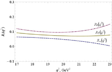
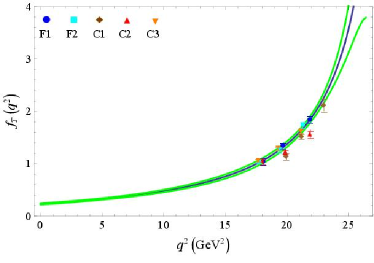
Figure 9: (Color online.) The $SU(3)_{F}$-symmetry breaking functions $R_{+}(q^{2})$, $R_{0}(q^{2})$ and $R_{T}(q^{2})$ (the upper plot) in the $q^{2}$-range accessible by the Lattice-QCD simulations and the tensor $B\to\pi$ transition form factor $f_{T}(q^{2})$ (the lower plot) in the entire kinematic region. The sets of vertical bars in the large-$q^{2}$ region are the preliminary results from the HPQCD Collaboration Bouchard et al. (2013c) presented at the Lattice-2013 Conference. The legend on the lower plot specifies the lattice ensembles as used in the $B\to K$ transitions Bouchard et al. (2013b) by the HPQCD Collaboration.

VI $B^{+}\to\pi^{+}\ell^{+}\ell^{-}$ Decay in Low-$q^{2}$ Region

VI.1 HQS Limit

As discussed in the Introduction, one can apply the heavy-quark symmetry techniques to relate the form factor $f_{T}(q^{2})$ in $B^{\pm}\to\pi^{\pm}\ell^{+}\ell^{-}$ to the measured form factor $f_{+}(q^{2})$ in the charged-current decay $B\to\pi\ell\nu_{\ell}$, in the large-recoil (or low-$q^{2}$) region. As shown in Ref. Beneke and Feldmann (2001), in the HQS limit (i. e., without taking into account symmetry-breaking corrections), $f_{0}(q^{2})$ and $f_{T}(q^{2})$ are proportional to $f_{+}(q^{2})$:

$$f_{0}(q^{2})=\frac{m_{B}^{2}-q^{2}}{m_{B}^{2}}\,f_{+}(q^{2}),$$ (64)

$$f_{T}(q^{2})=\frac{m_{B}+m_{\pi}}{m_{B}}\,f_{+}(q^{2}).$$ (65)

In the HQS limit, there is only one independent form factor $f_{+}(q^{2})$, the shape of which can be extracted from the analysis of the $B^{0}\to\pi^{-}\ell^{+}\nu_{\ell}$ and $B^{+}\to\pi^{0}\ell^{+}\nu_{\ell}$, which we presented in Sec. IV. The decay rate of $B^{+}\to\pi^{+}\ell^{+}\ell^{-}$ in the HQS limit is greatly simplified and takes the form:

$$\frac{d{\cal B}\left(B^{+}\to\pi^{+}\ell^{+}\ell^{-}\right)}{dq^{2}} = \frac{G_{F}^{2}\alpha_{\rm em}^{2}\tau_{B^{+}}}{1024\pi^{5}m_{B}^{3}}\,\left|V_{tb}V_{td}^{*}\right|^{2}\,$$

$$\times \sqrt{\lambda(q^{2})}\sqrt{1-\frac{4m_{\ell}^{2}}{q^{2}}}\,\tilde{F}(q^{2})\,f_{+}^{2}(q^{2}),$$

where the dynamical function $F(q^{2})$, defined in Eq. (II), is now reduced to the following expression:

$$\tilde{F}(q^{2}) = \frac{2}{3}\,\lambda(q^{2})\left(1+\frac{2m_{\ell}^{2}}{q^{2}}\right)\left|C_{9}^{\rm eff}(q^{2})+\frac{2m_{b}}{m_{B}}\,C_{7}^{\rm eff}(q^{2})\right|^{2}$$

$$+ \frac{2}{3}\,\lambda(q^{2})\left|C_{10}^{\rm eff}\right|^{2}+\frac{4m_{\ell}^{2}}{q^{2}}\left|C_{10}^{\rm eff}\right|^{2}$$

$$\times \left[\left(1-\frac{m_{\pi}^{2}}{m_{B}^{2}}\right)^{2}\left(m_{B}^{2}-q^{2}\right)^{2}-\frac{2}{3}\,\lambda(q^{2})\right],$$

and the kinematic function $\lambda(q^{2})$ is given in Eq. (13).

Table 5: Main input parameters used in the theoretical evaluations of the $B^{+}\to\pi^{+}\ell^{+}\ell^{-}$ branching fractions taken from the PDG Beringer et al. (2012), except for the $B$-meson leptonic decay constant $f_{B}$, whose value is taken from Lattice-NRQCD Dowdall et al. (2013).

$G_{F}=1.11637\times 10^{-5}\,\rm{GeV}^{-2}$	$\alpha_{\rm em}^{-1}=129$
$m_{B}=5.2792\,\rm{GeV}$	$\tau_{B^{+}}=1.641$ ps
$m_{\pi}=139.57\,\rm{MeV}$	$f_{\pi}=132$ MeV
$\alpha_{s}(M_{Z})=0.1184\pm 0.0007$	$f_{B}=(184\pm 4)$ GeV
$m_{c}(m_{c})=(1.275\pm 0.025)$ GeV	$m_{b}(m_{b})=(4.18\pm 0.03)$ GeV
$\lambda=0.22535\pm 0.00065$	$A=0.817\pm 0.015$
$\bar{\rho}=0.136\pm 0.018$	$\bar{\eta}=0.348\pm 0.014$
$|V_{ud}|=0.97427$	$|V_{tb}|=0.999146$
$|V_{ub}|=(3.51^{+0.15}_{-0.14})\times 10^{-3}$	$|V_{td}|=(8.67^{+0.29}_{-0.31})\times 10^{-3}$

Restricting ourselves to the NLL results for the effective Wilson coefficients (i. e., dropping the $\alpha_{s}(\mu)$-dependent terms in them) and using the $f_{+}(q^{2})$ form-factor shape extracted in terms of the BGL parametrization from the combined BaBar and Belle data, and the numerical values of the different quantities entering (VI.1) from Table 5, the numerical values of the $B^{\pm}\to\pi^{\pm}\mu^{+}\mu^{-}$ partial branching ratio in the ranges $4m_{\mu}^{2}\leq q^{2}\leq 8$ GeV² and $1~{}{\rm GeV}^{2}\leq q^{2}\leq 8$ GeV² are given below:

$$\begin{split}{\cal B}(B^{\pm}\to\pi^{\pm}\mu^{+}\mu^{-};\,0.05\,{\rm GeV}^{2}\leq q^{2}\leq 8\,{\rm GeV}^{2})&\\ =(0.80\pm 0.07)\times 10^{-8},&\end{split}$$ (68)

$$\begin{split}{\cal B}(B^{\pm}\to\pi^{\pm}\mu^{+}\mu^{-};\,1\,{\rm GeV}^{2}\leq q^{2}\leq 8\,{\rm GeV}^{2})&\\ =(0.72\pm 0.06)\times 10^{-8}.&\end{split}$$ (69)

VI.2 Including HQS-Breaking Correction

Heavy-quark symmetry, which holds in the large-recoil limit, allows one to get relations among the $B\to\pi$ form factors Charles et al. (1999). Taking into account the leading-order symmetry-breaking corrections, these relations were worked out in Ref. Beneke and Feldmann (2001):

$$f_{0}(q^{2}) = \left(1-\frac{q^{2}}{m_{B}^{2}}\right)f_{+}(q^{2})$$

$$\times \left\{1+\frac{C_{F}\alpha_{s}(\mu_{h})}{4\pi}\left[2-2L(q^{2})\right]\right\}$$

$$+ \frac{C_{F}\alpha_{s}(\mu_{hc})}{4\pi}\,\frac{q^{2}}{m_{B}^{2}-q^{2}}\,\Delta F_{\pi},$$

$$f_{T}(q^{2}) = \left(1+\frac{m_{\pi}}{m_{B}}\right)f_{+}(q^{2})$$

$$\times \left[1+\frac{C_{F}\alpha_{s}(\mu_{h})}{4\pi}\left(\ln\frac{m_{b}^{2}}{\mu_{h}^{2}}+2L(q^{2})\right)\right]$$

$$- \frac{C_{F}\alpha_{s}(\mu_{hc})}{4\pi}\,\frac{m_{B}\left(m_{B}+m_{\pi}\right)}{m_{B}^{2}-q^{2}}\,\Delta F_{\pi},$$

where $C_{F}=4/3$. The strong coupling $\alpha_{s}(\mu)$ depends on the specific scales of the contributing diagrams, which we take as the hard $\mu_{h}\sim m_{b}$ and hard-collinear $\mu_{hc}\sim\sqrt{m_{b}\Lambda}$ scales, where $\Lambda\simeq 0.5$ GeV is the typical soft hadronic scale. The auxiliary function $L(q^{2})$ is defined as follows Beneke and Feldmann (2001):

$$L(q^{2})=\left(1-\frac{m_{B}^{2}}{q^{2}}\right)\ln\left(1-\frac{q^{2}}{m_{B}^{2}}\right),$$ (72)

with the normalization $L(0)=1$, and the contributions of the hard-spectator diagrams are parametrized by the quantity Beneke and Feldmann (2001):

$$\Delta F_{\pi}=\frac{8\pi^{2}f_{B}f_{\pi}}{3m_{B}}\left\langle l_{+}^{-1}\right\rangle_{+}\left\langle\bar{u}^{-1}\right\rangle_{\pi}.$$ (73)

Here, $f_{B}$ and $f_{\pi}$ are the leptonic decay constants of the $B$- and $\pi$-mesons, respectively, and the following first inverse moments of the $B$- and $\pi$-mesons are used:

$$\left\langle l_{+}^{-1}\right\rangle_{+}=\int\limits_{0}^{\infty}dl_{+}\,\frac{\phi^{B}_{+}(l_{+})}{l_{+}},\quad\left\langle\bar{u}^{-1}\right\rangle_{\pi}=\int\limits_{0}^{1}du\,\frac{\phi_{\pi}(u)}{1-u},$$ (74)

which are completely determined by the leading-twist light-cone distribution amplitudes $\phi^{B}_{+}(l_{+})$ Grozin and Neubert (1997); Braun et al. (2004) and $\phi_{\pi}(u)$ Chernyak and Zhitnitsky (1977); Chernyak et al. (1977); Chernyak and Zhitnitsky (1980); Efremov and Radyushkin (1980a, b); Lepage and Brodsky (1979, 1980); Braun and Filyanov (1989); Ball (1999). With the input parameters $m_{B}$, $f_{B}$ and $f_{\pi}$ from Table 5, and the moments evaluated as $\left\langle\bar{u}^{-1}\right\rangle_{\pi}(1~{}{\rm GeV})=3.30\pm 0.42$ and $\left\langle l_{+}^{-1}\right\rangle_{+}(1.5~{}{\rm GeV})=(1.86\pm 0.17)$ GeV^-1 Lee and Neubert (2005), we estimate $\Delta F_{\pi}=0.74\pm 0.12$. This is numerically somewhat smaller than the value $\Delta F_{\pi}=1.17$ used in Ref. Beneke and Feldmann (2001). This difference reflects the observation that the $\pi$-meson is well described by the asymptotic form of the twist-2 LCDA $\phi_{\pi}(u)=6u\left(1-u\right)$, and the first subleading Gegenbauer moment $a_{2}(1~{}{\rm GeV})=0.10\pm 0.14$ Agaev et al. (2012) is consistent with zero.

Taking into account the symmetry-breaking corrections, and the NNLO effects in the effective Wilson coefficients, the partial branching fractions, integrated in the ranges of $q^{2}$ as in Eqs. (68) and (69), are decreased. We get

$$\begin{split}{\cal B}(B^{+}\to\pi^{+}\mu^{+}\mu^{-};\,0.05\,{\rm GeV}^{2}\leq q^{2}\leq 8\,{\rm GeV}^{2})&\\ =(0.65^{+0.08}_{-0.06})\times 10^{-8},&\end{split}$$ (75)

$$\begin{split}{\cal B}(B^{+}\to\pi^{+}\mu^{+}\mu^{-};\,1\,{\rm GeV}^{2}\leq q^{2}\leq 8\,{\rm GeV}^{2})&\\ =(0.57^{+0.07}_{-0.05})\times 10^{-8},&\end{split}$$ (76)

which mainly reflects the NNLO effects in the Wilson coefficients. The corresponding dilepton invariant-mass distribution in the large-recoil approximation ($q^{2}\leq 8$ GeV²) is shown in Fig. 10. The vertical line shows the light-resonance ($\rho$, $\omega$, and $\phi$) region collectively. The upper bound on $q^{2}$ is imposed to avoid the large (resonant) contribution from the long-distance process $B^{\pm}\to\pi^{\pm}\,J/\psi\to\pi^{\pm}\ell^{+}\ell^{-}$.

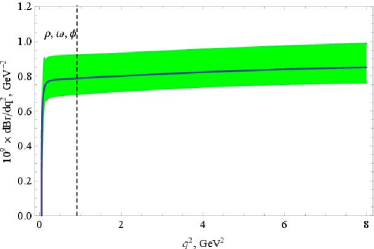
Figure 10: (Color online.) The dilepton invariant-mass distribution $d{\cal B}(B^{\pm}\to\pi^{\pm}\ell^{+}\ell^{-})/dq^{2}$ for $0\leq q^{2}\leq 8$ GeV² calculated by taking into account the leading HQS-breaking corrections. Dashed vertical line indicates collectively the vector $\rho$-, $\omega$-, and $\phi$-resonance region.

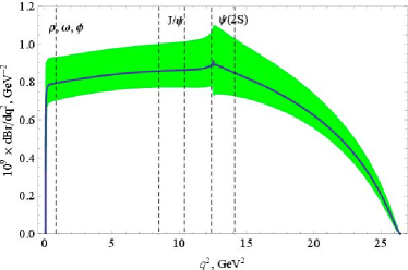
Figure 11: (Color online.) The dilepton invariant-mass distribution in the $B^{+}\to\pi^{+}\ell^{+}\ell^{-}$ decay for the entire kinematic range $0\leq q^{2}\leq 26.4$ GeV². Dashed vertical lines specify the positions of vector resonances: $\rho$-, $\omega$- and $\phi$-mesons at $q^{2}\lesssim 1$ GeV² and $J/\psi$- and $\psi(2S)$-mesons near $q^{2}\simeq 9.5$ GeV² and $q^{2}\simeq 13.5$ GeV², respectively.

Table 6: Partial branching ratios $d{\cal B}(B^{+}\to\pi^{+}\mu^{+}\mu^{-})/dq^{2}$ integrated over the indicated ranges $[q^{2}_{\rm min},q^{2}_{\rm max}]$.

$[q^{2}_{\rm min},q^{2}_{\rm max}]$	$10^{8}\times{\cal B}(q^{2}_{\rm min}\leq q^{2}\leq q^{2}_{\rm max})$
$[0.05,2.0]$	$0.15^{+0.03}_{-0.02}$
$[1,2.0]$	$0.08^{+0.01}_{-0.01}$
$[2.0,4.3]$	$0.19^{+0.03}_{-0.02}$
$[4.3,8.68]$	$0.37^{+0.06}_{-0.04}$
$[10.09,12.86]$	$0.25^{+0.04}_{-0.03}$
$[14.18,16.0]$	$0.15^{+0.03}_{-0.02}$
$[16.0,18.0]$	$0.15^{+0.03}_{-0.02}$
$[18.0,22.0]$	$0.25^{+0.04}_{-0.03}$
$[22.0,26.4]$	$0.13^{+0.02}_{-0.02}$
$[0.05,8.0]$	$0.66^{+0.10}_{-0.07}$
$[1.0,8.0]$	$0.58^{+0.09}_{-0.06}$
$[4m_{\mu}^{2},(m_{B}-m_{\pi})^{2}]$ (total)	$1.88^{+0.32}_{-0.21}$

VI.3 Estimating the $SU(3)_{F}$-Breaking
in the $B\to\pi,K$ Tensor Form Factors

Before presenting the estimates of the $B^{+}\to\pi^{+}\ell^{+}\ell^{-}$ branching fraction in the entire kinematic range of $q^{2}$, we would like to discuss the validity of the Ansatz (60) used by us in calculating the $SU(3)_{F}$-breaking effects in the $B\to\pi,K$ tensor form factors. The accuracy of our Ansatz can be easily determined in the kinematic region where the HQS-based methods apply. These will be worked out below and used to project also the accuracy in the large-$q^{2}$ region. We note that the lattice data already provides a reliable estimate of the r.h.s. of Eq. (60), but only preliminary lattice data Bouchard et al. (2013c) are available for the l.h.s., involving the tensor form factors.

Taking into account the leading-order HQS-symmetry-breaking effects, all three $B\to P$ transition form factors, where $P$ is a light pseudoscalar meson, are related, as shown in Eqs. (VI.2) and (VI.2). This then allows one to relate the $SU(3)_{F}$-symmetry breaking measures:

$$R_{0}(q^{2})=R_{+}(q^{2})\left[1+\frac{C_{F}\alpha_{s}(\mu_{hc})}{4\pi}\,\right.$$ (77)

$$\hskip 42.67912pt\left.\times\frac{q^{2}/m_{B}^{2}}{\left(1-q^{2}/m_{B}^{2}\right)^{2}}\,\left(\frac{\Delta F_{K}}{f_{+}^{BK}(q^{2})}-\frac{\Delta F_{\pi}}{f_{+}^{B\pi}(q^{2})}\right)\right],$$

$$R_{T}(q^{2})=\frac{1+m_{K}/m_{B}}{1+m_{\pi}/m_{B}}\,R_{+}(q^{2})\left[1-\frac{C_{F}\alpha_{s}(\mu_{hc})}{4\pi}\qquad\right.$$ (78)

$$\hskip 42.67912pt\left.\times\frac{1}{1-q^{2}/m_{B}^{2}}\,\left(\frac{\Delta F_{K}}{f_{+}^{BK}(q^{2})}-\frac{\Delta F_{\pi}}{f_{+}^{B\pi}(q^{2})}\right)\right],$$

where

$$f_{+}^{BK}(q^{2})=f_{+}^{B\pi}(q^{2})\left[1+R_{+}(q^{2})\right],$$ (79)

and

$$\Delta F_{K} = \Delta F_{\pi}\,\frac{f_{K}}{f_{\pi}}\,\frac{\langle\bar{u}^{-1}\rangle_{K}}{\langle\bar{u}^{-1}\rangle_{\pi}}$$

$$\simeq \Delta F_{\pi}\left(1+\Delta f_{K\pi}\right)\left[1+a_{1}^{K}(\mu_{hc})\right].$$

Here $\Delta f_{K\pi}=f_{K}/f_{\pi}-1\simeq 0.23$ is the $SU(3)_{F}$-symmetry breaking in the leptonic decay constants ($f_{\pi}\simeq 130$ MeV and $f_{K}\simeq 160$ MeV Beringer et al. (2012)). The first inverse moments of the $K$- and $\pi$-mesons $\langle\bar{u}^{-1}\rangle_{P}(\mu_{hc})\simeq 3\left[1+a_{1}^{P}(\mu_{hc})\right]$ are approximated by the asymptotic and the first Gegenbauer terms in the conformal expansion of the LCDAs with $a_{1}^{\pi}(2~{}{\rm GeV})=0$ and $a_{1}^{K}(2~{}{\rm GeV})=0.05\pm 0.02$ Ball and Zwicky (2006); Ball et al. (2007) (the other terms in the Gegenbauer decomposition do not affect the ratio $\Delta F_{K}/\Delta F_{\pi}$ significantly). Keeping terms linear in $\Delta f_{K\pi}$, $a_{1}^{K}(\mu_{hc})$ and $R_{+}(q^{2})$ only in the hard-collinear correction, the measures of the $SU(3)_{F}$-symmetry breaking become:

$$R_{0}(q^{2})=R_{+}(q^{2})\left\{1+\frac{C_{F}\alpha_{s}(\mu_{hc})}{4\pi}\,\right.$$ (81)

$$\hskip 14.22636pt\left.\times\frac{\hat{q}^{2}\,\Delta F_{\pi}}{\left(1-\hat{q}^{2}\right)^{2}f_{+}^{B\pi}(q^{2})}\left[\Delta f_{K\pi}+a_{1}^{K}(\mu_{hc})-R_{+}(q^{2})\right]\right\},$$

$$R_{T}(q^{2})=\frac{1+\hat{m}_{K}}{1+\hat{m}_{\pi}}\,R_{+}(q^{2})\left\{1-\frac{C_{F}\alpha_{s}(\mu_{hc})}{4\pi}\,\right.$$ (82)

$$\hskip 14.22636pt\left.\times\frac{\Delta F_{\pi}}{\left(1-\hat{q}^{2}\right)f_{+}^{B\pi}(q^{2})}\left[\Delta f_{K\pi}+a_{1}^{K}(\mu_{hc})-R_{+}(q^{2})\right]\right\},$$

where the reduced mass $\hat{m}_{P}=m_{P}/m_{B}$ ($P=\pi,\,K$) and the reduced momentum transfer squared is defined as $\hat{q}^{2}=q^{2}/m_{B}^{2}$. With $\hat{m}_{\pi}=0.0265$ and $\hat{m}_{K}=0.0947$ Beringer et al. (2012), their difference $\hat{m}_{K}-\hat{m}_{\pi}=0.0682$ yields $(1+\hat{m}_{K})/(1+\hat{m}_{\pi})=1.07$ for the prefactor on the r.h.s. of Eq. (82).

To quantify the validity of the Ansatz (60), let us introduce the following function:

$$\Delta R(q^{2})=\frac{1}{2}\left[R_{+}(q^{2})+R_{0}(q^{2})\right]-R_{T}(q^{2}),$$ (83)

whose deviation from zero quantitatively determines the accuracy of our $SU(3)_{F}$-breaking Ansatz. Using Eqs. (81) and (82), $\Delta R(q^{2})$ can be estimated as follows:

$$\Delta R(q^{2})\simeq R_{+}(q^{2})\left\{\hat{m}_{\pi}-\hat{m}_{K}+\frac{C_{F}\alpha_{s}(\mu_{hc})}{4\pi}\,\right.$$ (84)

$$\hskip 8.53581pt\left.\times\frac{\left(1-\hat{q}^{2}/2\right)\Delta F_{\pi}}{\left(1-\hat{q}^{2}\right)^{2}f_{+}^{B\pi}(q^{2})}\left[\Delta f_{K\pi}+a_{1}^{K}(\mu_{hc})-R_{+}(q^{2})\right]\right\}.$$

There are two competitive contributions: the first one is coming from the reduced mass difference, and the second one combines the perturbative corrections in the form factors (the HQS-breaking corrections due to the hard-spectator contributions).

To remove the term induced by the $K$- and $\pi$-meson difference from $\Delta R(q^{2})$, we define a reduced function $\tilde{R}_{T}(q^{2})$ as follows:

$$\tilde{R}_{T}(q^{2})\equiv\frac{m_{B}+m_{\pi}}{m_{B}+m_{K}}\,\frac{f_{T}^{BK}(q^{2})}{f_{T}^{B\pi}(q^{2})}-1,$$ (85)

and a reduced analogue of the $\Delta R(q^{2})$ function:

$$\Delta\tilde{R}(q^{2})\equiv\frac{1}{2}\left[R_{+}(q^{2})+R_{0}(q^{2})\right]-\tilde{R}_{T}(q^{2}).$$ (86)

In the low-$q^{2}$ region (say, $0\leq q^{2}\leq 14$ GeV² or $0\leq\hat{q}^{2}\leq 1/2$), the deviation of this function from zero is completely determined by the hard-spectator corrections in the form factors:

$$\Delta\tilde{R}(q^{2})\simeq R_{+}(q^{2})\,\frac{C_{F}\alpha_{s}(\mu_{hc})}{4\pi}\,$$ (87)

$$\hskip 19.91692pt\times\frac{\left(1-\hat{q}^{2}/2\right)\Delta F_{\pi}}{\left(1-\hat{q}^{2}\right)^{2}f_{+}^{B\pi}(q^{2})}\left[\Delta f_{K\pi}+a_{1}^{K}(\mu_{hc})-R_{+}(q^{2})\right].$$

The input parameters are as follows: $C_{F}=4/3$, the hard-collinear scale $\mu_{hc}=2$ GeV, $\alpha_{s}(m_{\tau})=0.330\pm 0.014$ Beringer et al. (2012), $\left(1-\hat{q}^{2}\right)f_{+}^{B\pi}(q^{2})\simeq f_{+}^{B\pi}(0)=0.260\pm 0.014$ (our estimate), $\Delta F_{\pi}=0.74\pm 0.12$ (our estimate), $\Delta f_{K\pi}=f_{K}/f_{\pi}-1=0.23$ Beringer et al. (2012), $a_{1}^{K}(2~{}{\rm GeV})=0.05\pm 0.02$ Ball and Zwicky (2006); Ball et al. (2007). In addition, we need to know $R_{+}(q^{2})$. Ignoring the mild $q^{2}$-dependence, we set $R_{+}(q^{2})\simeq R_{+}(0)$, and discuss some representative estimates of $R_{+}(0)$. The most recent lattice result for the $B\to K$ vector form factor is by the HPQCD Collaboration Bouchard et al. (2013a, b) $f_{+}^{BK}(0)=0.319\pm 0.066$. With the determination of the corresponding quantity in the $B\to\pi$ transition, $f_{+}^{B\pi}(0)=0.260\pm 0.014$, we get $R_{+}(0)=0.231\pm 0.262$ (the error is dominated by the uncertainty in $f_{+}^{BK}(0)$). Another recent estimate $f_{+}^{BK}(0)=0.33\pm 0.04$ Becirevic et al. (2012) yields $R_{+}(0)=0.269\pm 0.169$, where again the error is mainly due to $f_{+}^{BK}(0)$. Note that the LCSR estimate $f_{+}^{BK}(0)=0.34^{+0.05}_{-0.02}$ Khodjamirian et al. (2010) is compatible with the above lattice predictions within the uncertainties. After the insertion of the lattice estimates in Eq. (87), the results are as follows:

$$\Delta\tilde{R}(q^{2})\simeq\frac{1-\hat{q}^{2}/2}{1-\hat{q}^{2}}\left\{\begin{array}[]{ll}(1.15\pm 2.19)\times 10^{-3},&\text{\cite[cite]{\@@bibref{Authors Phrase1YearPhrase2}{Bouchard:2013mia,Bouchard:2013eph}{\@@citephrase{(}}{\@@citephrase{)}}}}\\ (0.31\pm 1.58)\times 10^{-3}.&\text{\cite[cite]{\@@bibref{Authors Phrase1YearPhrase2}{Becirevic:2012fy}{\@@citephrase{(}}{\@@citephrase{)}}}}\end{array}\right.$$ (88)

So, the effect of the hard-scattering corrections is below 1% in the kinematic domain considered.

Coming back to the numerical evaluation of $\Delta R(q^{2})$, defined in (83), using the estimates (88) given above, one obtains:

$$\Delta R(q^{2}) \simeq R_{+}(q^{2})\left(\hat{m}_{\pi}-\hat{m}_{K}\right)$$ (89)

$$\simeq \left\{\begin{array}[]{ll}(-1.55\pm 1.76)\times 10^{-2},&\text{\cite[cite]{\@@bibref{Authors Phrase1YearPhrase2}{Bouchard:2013mia,Bouchard:2013eph}{\@@citephrase{(}}{\@@citephrase{)}}}}\\ (-1.81\pm 1.13)\times 10^{-2}.&\text{\cite[cite]{\@@bibref{Authors Phrase1YearPhrase2}{Becirevic:2012fy}{\@@citephrase{(}}{\@@citephrase{)}}}}\end{array}\right.$$ (92)

So, the uncertainty of the Ansatz (60) can be evaluated to be approximately 3% in the considered range of $q^{2}$.

The estimates presented above support the Ansatz (60) within an accuracy of about 3%. To which degree of accuracy, this Ansatz also holds in the high-$q^{2}$ domain will be tested as the lattice calculations of all the $B\to\pi$ transition form factors become completely quantitative. We include an additional error of 5%, ascribed to the error on the Ansatz (60) in the determination of the tensor form factor $f_{T}^{B\pi}(q^{2})$.

VII $B^{+}\to\pi^{+}\ell^{+}\ell^{-}$ Decay in the Entire $q^{2}$-Range

In the low hadronic-recoil region (large-$q^{2}$), heavy-quark symmetry does not hold, and we have three independent form factors $f_{+}(q^{2})$, $f_{0}(q^{2})$ and $f_{T}(q^{2})$ in $B^{\pm}\to\pi^{\pm}\ell^{+}\ell^{-}$. We have given a detailed account of their determination in the preceding sections. The vector form factor $f_{+}(q^{2})$ is determined taking into account the Belle and BaBar data on $B\to\pi\ell\nu_{\ell}$, and fitting several parametrizations, with the BGL-parametrization as our default choice. We have used the HQS-based method, including the leading-order symmetry breaking, in the low-$q^{2}$ region ($q^{2}\leq 8$ GeV²), and the experimentally constrained form factor $f_{+}(q^{2})$ to determine the other two form factors $f_{0}(q^{2})$ and $f_{T}(q^{2})$. Finally, we have used the available Lattice-QCD results for the form factors $f_{i}^{BP}(q^{2})$ $(i=+,0,T)$ in the large-$q^{2}$ region, obtained for the $B\to K$ and $B\to\pi$ transitions. As the lattice data on $f_{T}^{B\pi}(q^{2})$ is still sparse, we have determined this form factor from the lattice data on $f_{T}^{BK}(q^{2})$, and an Ansatz for the $SU(3)_{F}$-breaking. We have tested the accuracy of this Ansatz in the low-$q^{2}$ region, and find it to hold within 3%. This dedicated study has removed the largest source of theoretical uncertainty originating from the form factors.

Before presenting our numerical results, we discuss the choice for the parameter $\sqrt{z}=m_{c}/m_{b}$ entering the NNLO corrections. The NNLO corrections to the $b\to s\,\ell^{+}\ell^{-}$ transition matrix element Greub et al. (2008), which we have adapted for the exclusive $b\to d\,\ell^{+}\ell^{-}$ case discussed by us here, are available in the literature both as the Mathematica and the C++ programs Greub et al. (2008), from which the former one was implemented in our own Mathematica routine. We need to fix this ratio in terms of the $c$- and $b$-quark pole masses. The three-loop relation between the pole $m_{\rm pole}$ and $\overline{\rm MS}$-scheme $\bar{m}(\bar{m})$ masses Chetyrkin and Steinhauser (1999, 2000); Melnikov and Ritbergen (2000) can be used to get the $c$- and $b$-quark pole masses. Staring from the values collected in Table 5, the ratio $m_{c}(m_{c})/m_{b}(m_{b})=0.305\pm 0.006$ can be transformed into the ratio of the pole masses $m_{c,{\rm pole}}/m_{b,{\rm pole}}=0.402\pm 0.008$. In Xing et al. (2008), additional electroweak corrections to the relation between the pole and the $\overline{\rm MS}$ quark masses were taken into account with the resulting pole masses: $m_{c,{\rm pole}}=1.77\pm 0.14$ GeV and $m_{b,{\rm pole}}=4.91\pm 0.12$ GeV, with the ratio $m_{c,{\rm pole}}/m_{b,{\rm pole}}=0.36\pm 0.03$. This value is used by us as input for $\sqrt{z}$ in calculating the $c$-quark loop-induced corrections.

The invariant-mass spectrum in the entire range of $q^{2}$ ($4m_{\ell}^{2}<q^{2}<26.4$ GeV²) is presented in Fig. 11. Once again, we emphasize that this represents only the short-distance contribution. The dashed vertical lines specify the light-meson resonant region, shown at $q^{2}\lesssim 1$ GeV², as well as of the $J/\psi$- and $\psi(2S)$-mesons. In the calculation of this spectrum, Wilson coefficients are used in the NNLO accuracy. In the perturbative improvement, the auxiliary functions $F_{1,2}^{(7)}(q^{2})$ and $F_{1,2}^{(9)}(q^{2})$ entering the next-to-leading correction in $C_{9}^{\rm eff}(q^{2})$ are known analytically as power expansions in $s=q^{2}/m_{B}^{2}$ and in $1-s$ (as shown in Fig. 2). As explained earlier, we have extrapolated these functions into the intermediate $q^{2}$-region. In doing this, we have matched the known analytical functions in the form of expansions at the “matching” point $q^{2}\simeq 12.5$ GeV², at which value the spectrum has the minimal discontinuity (see Fig. 11). This yields an invariant-mass spectrum which is a smooth function of $q^{2}$, within uncertainties. It is important to note that the “matching” point $q^{2}\simeq 12.5$ GeV² lies in the $\psi(2S)$-resonance region which is dominated by the long-distance effects. Away from the resonance regions, the short-distance contribution to the differential branching fraction dominates and the discontinuity in the spectrum discussed earlier is not a crucial issue.

Our predictions for the partial branching fractions $d{\cal B}(B^{\pm}\to\pi^{\pm}\,\ell^{+}\ell^{-})/dq^{2}$ in eleven different $q^{2}$ bins are presented in Table 6. The total branching fraction of the semileptonic $B^{\pm}\to\pi^{\pm}\,\mu^{+}\mu^{-}$ decay is as follows:

$$\begin{split}&{\cal B}(B^{\pm}\to\pi^{\pm}\,\mu^{+}\mu^{-})\\ &\quad=\left(1.88^{+0.28}_{-0.15}\big{|}_{\mu_{b}}\pm 0.13\big{|}_{|V_{td}|}\pm 0.08\big{|}_{\rm FF}\pm 0.01\right)\times 10^{-8}\\ &\hskip 28.45274pt=\left(1.88^{+0.32}_{-0.21}\right)\times 10^{-8},\end{split}$$ (93)

where the individual uncertainties are from the scale dependence $\mu_{b}$ of the Wilson coefficients, the CKM matrix element $|V_{td}|$, and the form factors (FF), as indicated. The resulting average uncertainty is about 15%, which is dominated by the scale dependence of the Wilson coefficients and can be reduced after the scale-dependence of the tensor form factor $f^{B\pi}_{T}(q^{2})$ is worked out properly in the entire $q^{2}$-range.

The branching fraction for the semileptonic $B^{\pm}\to\pi^{\pm}\,e^{+}e^{-}$ decay is the same as (93), as the additional contribution induced by the shift to the lower kinematic values of $q^{2}=4m_{e}^{2}\simeq 1$ MeV² is negligible.

The use of the isospin symmetry allows to make predictions for the $B^{0}\to\pi^{0}\,\ell^{+}\ell^{-}$ decay also. Neglecting the effects of the isospin symmetry breaking in the $B\to\pi$ transition form factors which are expected to be a few percent, the main modification is the isospin factor $C_{\pi^{0}}=1/2$ in the final state due to the $\pi^{0}$-meson structure. Taking this into account, our predictions for the partial branching fractions are as follows:

$$\begin{split}{\cal B}(B^{0}\to\pi^{0}\ell^{+}\ell^{-};\,0.05\,{\rm GeV}^{2}\leq q^{2}\leq 8\,{\rm GeV}^{2})&\\ =(0.33^{+0.05}_{-0.03})\times 10^{-8},&\end{split}$$ (94)

$$\begin{split}{\cal B}(B^{0}\to\pi^{0}\ell^{+}\ell^{-};\,1\,{\rm GeV}^{2}\leq q^{2}\leq 8\,{\rm GeV}^{2})&\\ =(0.29^{+0.05}_{-0.03})\times 10^{-8},&\end{split}$$ (95)

where $\ell=e$ or $\mu$, and for the total branching fraction we estimate:

$${\cal B}(B^{0}\to\pi^{0}\,\ell^{+}\ell^{-})=\left(0.94^{+0.16}_{-0.11}\right)\times 10^{-8}.$$ (96)

The above decay rates ${\cal B}(B^{0}\to\pi^{0}\,\ell^{+}\ell^{-})$ will be measured at the forthcoming Super-B factory at KEK.

VIII Summary and Outlook

We have presented a theoretically improved calculation of the branching fraction for the $B^{\pm}\to\pi^{\pm}\mu^{+}\mu^{-}$ decay, measured recently by the LHCb Collaboration Aaij et al. (2012). In doing this, we have used the effective Wilson coefficients $C_{7}^{\rm eff}(q^{2})$, $C_{9}^{\rm eff}(q^{2})$ and $C_{10}^{\rm eff}$, obtained in the NNLO accuracy earlier for the $b\to(s,\,d)\,\ell^{+}\ell^{-}$ decays Bobeth et al. (2000); Asatrian et al. (2001); Asatryan et al. (2002); Ali et al. (2002); Asatrian et al. (2004). Some of the auxiliary functions, called $F_{1,2}^{(7)}(q^{2})$, $F_{1,2}^{(9)}(q^{2})$, $F_{1,(2),u}^{(7)}(q^{2})$, $F_{1,(2),u}^{(9)}(q^{2})$ are known analytically in the limiting case of $m_{c}/m_{b}=0$ Seidel (2004), which we have used. For realistic values of this ratio, taken by us as $\sqrt{z}=m_{c}/m_{b}=0.36$, the results are known only in limited ranges of $s=q^{2}/m_{B}^{2}$ ($s\leq 0.35$ and $0.55<s<1.0$). All these functions are shown numerically in Fig. 2. We have interpolated in the gap, which introduces some uncertainty, but being part of the NNLO contribution, it is not expected to be the dominant error. Theoretical uncertainties are dominated by the imprecise knowledge of the form factors, $f_{+}^{B\pi}(q^{2})$ and $f_{T}^{B\pi}(q^{2})$. We have extracted the shape of the former from data on the charged-current process $B\to\pi\ell\nu_{\ell}$, measured at the $B$-factories. Among the four popular parametrizations, the BGL (Boyd, Grinstein and Lebed) $z$-expansion was chosen as our working tool. For the tensor form factor $f_{T}^{B\pi}(q^{2})$, heavy-quark symmetry provides the information in the low-$q^{2}$ (large-recoil) region, in which this form factor is related to the known factor $f_{+}^{B\pi}(q^{2})$, up to symmetry-breaking effects, which we have estimated from the existing literature. This provides us an estimate of the dilepton invariant-mass spectrum for $q^{2}\leq 8$ GeV². For larger values of $q^{2}$, we have used the $SU(3)_{F}$-symmetry-breaking Ansatz and knowledge of the form factor $f_{T}^{BK}(q^{2})$ from lattice QCD. Comparison with the preliminary results by the HPQCD Collaboration studies of the form factor $f_{T}^{B\pi}(q^{2})$ in the low-recoil (or large-$q^{2}$) region Bouchard et al. (2013c) shows a good consistency with our results. This then provides us a trustworthy profile of the two form factors needed in estimating the entire dilepton invariant-mass spectrum and the partial branching ratio. The combined accuracy on the branching ratio is estimated as $\pm 15\%$, and the resulting branching fraction ${\cal B}(B^{\pm}\to\pi^{\pm}\mu^{+}\mu^{-})=(1.88^{+0.32}_{-0.21})\times 10^{-8}$ is in agreement with the LHCb data Aaij et al. (2012). We have provided partial branching fractions in different ranges of $q^{2}$, which can be compared directly with the data, as and when they become available.

Note added in Proofs. Recently, the analysis of the $B\to\pi\ell\bar{\ell}$ and $B\to\pi\rho\bar{\ell}$ decays in the relativistic quark model has been presented in Ref. Faustov and Galkin (2014). The main difference in comparison with our analysis is that the $B\to\pi$ transition form factors were determined theoretically by utilizing the relativistic quark model based on the quasipotential approach and QCD. The total branching fraction ${\cal B}(B^{\pm}\to\pi^{\pm}\mu^{+}\mu^{-})=(2.0\pm 0.2)\times 10^{-8}$ is in good agreement with our result.