Diffusion coefficients from signal fluctuations:
Influence of molecular shape and rotational diffusion

Abstract

Analysis of signal fluctuations of a locally fixed probe, caused by molecules diffusing under the probe, can be used to determine diffusion coefficients. Theoretical treatments so far have been limited to point-like particles or to molecules with circle-like shapes. Here we extend these treatments to molecules with rectangle-like shapes, for which also rotational diffusion needs to be taken into account. Focusing on the distribution of peak widths in the signal, we show how translational as well as rotational diffusion coefficients can be determined. We address also the question, how the distribution of interpeak time intervals and autocorrelation function can be employed for determining diffusion coefficients. Our approach is validated against kinetic Monte Carlo simulations.

I Introduction

Self-assembly of molecules on surfaces has become a topic of intensive research, both from a fundamental point of view and for developing electronics based on molecular units.Rahe et al. (2013); Hlawacek and Teichert (2013); Einax et al. (2013); Kühnle (2009); Kowarik et al. (2008) For controlling the kinetic growth, the diffusion coefficient is an important parameter. Various techniques are used to measure molecular diffusion on surfaces.Barth (2000) For fast diffusion, a particularly suited method is an analysis of signal fluctuations caused by molecules entering and leaving the detection area under a probe. Corresponding time series can be recorded by a scanning tunneling microscope, Lozano and Tringides (1995) or, in principle, also by an atomic force microscope or some other probe with a point like sensor. By fixing the probe locally above the substrate, the time resolution can be significantly increased, thus allowing to capture high mobilities, as often encountered in the case of molecular motion.

Different means are available for evaluating the detection events in the time series. Originally, the autocorrelation function (ACF) has been the focus of experimental Tringides et al. (1999) and theoretical Sumetskii and Kornyshev (1993) studies. For atomic diffusion, the ACF method yields relative changes of diffusion coefficients $D$. Recently, this method has been extended to molecules with sizes larger than the step length of translational moves.Hahne et al. (2013) This way absolute values of $D$ become accessible. Furthermore, the residence time-distributionIkonomov et al. (2010) (RTD) has been discussed and another new method, the interpeak-time distribution (ITD), has been introduced. The RTD is the distribution of peak widths and the ITD is the distribution of time intervals between successive peaks. Both of them are suitable to determine absolute values of $D$.

Various merits and limits have been discussed for the three variants based on the ACF, RTD, and ITD.Hahne et al. (2013) From a general point of view, inter-molecular and molecule-tip interactions can affect the results. The ACF is influenced by both of these interactions, while the ITD is influenced only by inter-molecular interactions. Accordingly, the RTD method can be viewed as the most powerful one, because it is only influenced by the molecule-tip interaction, which can be reduced systematically by adjusting the molecule-probe distance.Ikonomov et al. (2010)

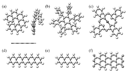
Figure 1: Ground-state vacuum structures obtained from density functional calculations of several molecules. These molecules can be viewed as representative for classes of derivatives that are widely used in studies of molecular self-assembly on surfaces: (a) heliceneSeibel et al. (2013) (top and side view), (b) hexaphenylbenzene,Gross et al. (2005) (c) (copper-) phtalocyanine,Mugarza et al. (2012) (d) pentacenceGross et al. (2009) (e) anthracene,Wan and Itaya (1997); Potapenko et al. (2010) and (f) the perylene derivate PTCDA.Paulheim et al. (2013) Images of the molecules in the respective studies suggest that their overall shape is not significantly distorted upon adsorption and that they often lie flat on the surface. Circular and rectangular shapes can hence be expected to describe their detection area under the probe to a good approximation.

So far, the focus lay on molecules, whose shape can be effectively described by a circle. Examples of such circular-type molecules, widely used in present studies of self-assembly on surfaces, are shown in Fig. 1(a)-(c). Other molecules in such studies, as shown in Fig. 1(d)-(f), are better described by rectangles. In this work, we extend our theoretical treatment to these shapes. Rectangular-type molecule render signal fluctuations from rotational diffusion possible. Including such rotational moves in the theoretical description increases the complexity significantly. We offer a first approach to this problem, considering thermally activated rotational diffusion uncoupled from translation. Our focus in this work will be on the RTD, because of its advantage over the other methods. In the last section VI, we will also adress the question how rectangular shapes and rotational diffusion affect the ACF and ITD. As a further point, we discuss in Sec. III the question how many peaks need to be recorded to obtain faithful results for the diffusion coefficient.

II KMC simulations

The quality of approximations entering our analytical treatments is checked by comparison with results obtained from kinetic Monte Carlo (KMC) simulations. These simulations are carried out on a square lattice with lattice constant $a=1$ (setting our length unit) and periodic boundary conditions. The center positions of $N$ particles of circular or rectangular shape perform jumps between nearest neighbor lattice sites with rate $w_{D}=4D/a^{2}=1$ ($w_{D}^{-1}$ setting our time unit), where $D$ is the diffusion coefficient. The latter is to be compared to $\tilde{D}$ values extracted from the analysis of simulated data, which serve as surrogate for experimental ones. The particles represent freely diffusing molecules in an experiment and are assumed to have a coverage much smaller than a monolayer. We are neglecting any interaction effects between them. When including rotational dynamics, reorientation moves with rate $w_{\varphi}$ are additionally taken into account, see Sec. V. Translational and rotational dynamics are implemented by using the reaction time algorithm.Holubec et al. (2011)

Figure 2: Part of a simulated “on-off” time series. Peak widths are denoted by $t$.

Time series are generated by selecting one fixed lattice site, the so-called “probe-site”, which represents the point on the surface, from which the signal in an experiment is recorded. The simulated signal is “on” if the probe-site is covered by a part of a molecule, while otherwise it is “off”. The thus-generated “on-off” time series resemble measured ones, if in the latter noise is eliminated and a proper threshold is set, which allows for a reduction to a rectangular signal. The details of this procedure are described in Ref. Hahne et al., 2013. The example shown in Fig. 2(b) of that work may be compared to the simulated signal displayed in Fig. 2.

III RTD for molecules with circular shapes

In the following we shortly summarize our previous results from Ref. Hahne et al., 2013 with respect to the RTD, because we will refer repeatedly to the corresponding equations in the following sections. The methods were developed for molecules, with size large compared to the sensitive area of the probe. This way the probe can be considered as pointlike and the molecule extension gives rise to a detection area, which is defined by the set of molecule center positions around the tip, that will cause a detectable change in the signal. For molecules with approximately circular shapes, as the ones shown in Fig. 1(a)-(c), a circle with radius $R$ can be assigned to the detection area, for example, by taking its gyration radius. The RTD then is given by

$$\Psi_{\rm circ}(t)=\frac{2D}{R^{2}}\sum_{n=1}^{\infty}\frac{x_{n}~{}J_{0}(x_{n}(1-\frac{\Delta}{R}))}{J_{1}(x_{n})}\,\textrm{e}^{-x_{n}^{2}Dt/R^{2}}\,,$$ (1)

where $J_{\nu}(.)$ is the Bessel function of first kind with $x_{n}$ its $n$-th zero; $\Delta$ is the minimal penetration depth of the center into the detection area under the tip, which is at least necessary to turn the signal “on”. For times much larger than the typical time $\tau_{R}\equiv R^{2}/(x_{1}^{2}D)$ for the molecule to explore the detection area,

$$\Psi_{\rm circ}\left(t\right)\sim\frac{2D}{R^{2}}\frac{x_{1}~{}J_{0}(x_{1}(1-\frac{\Delta}{R}))}{J_{1}(x_{1})}\,\textrm{e}^{-x_{1}^{2}Dt/R^{2}}\,,$$ (2)

while a power law $\sim t^{-3/2}$ characterizes the behavior for $\Delta^{2}/D\ll t\ll\tau_{R}$. For $t\lesssim\Delta^{2}/D$ the continuum description breaks down.

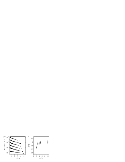
Figure 3: (a) Simulated RTDs for various fractions $R/\Delta=1$ ($\lhd$), 2 ($\diamond$), 3 ($\square$), 4 ($\circ$), 5 ($\star$), and 10 ($\bullet$). The dashed lines are least square fits to Eq. (2). The distributions were vertically shifted for better visibility. (b) Diffusion coefficients $\tilde{D}$ from the fitting, divided by the input value $D$ in the KMC simulation, as a function of $R/\Delta$.

Application of Eq. (1) and its derivates requires $R/\Delta$ to exceed a certain threshold, because for $\Delta$ close to or larger than $R$, one would need to consider molecular jumps into and out of the detection area instead of a diffusive motion within this area. The jump motion could be treated as well, but this is not our focus here. Corresponding events may be difficult to detect within experimental time resolution. Nevertheless, before starting to address our main topics, it is interesting to see, down to which fractions $R/\Delta$ the continuum treatment gives reliable results for $D$. Simulated RTDs for various fractions $R/\Delta$ are shown in Fig. 3 and were fitted with Eq. (2). In these simulations we fixed $\Delta$ and $D$, and varied $R$. The fits [dashed lines in Fig. 3(a)] yield estimates $\tilde{D}$ in good agreement with $D$ for $R/\Delta\gtrsim 3$, see Fig. 3(b).

Figure 4: (a) Simulated RTDs for various total numbers of events $N=$ 10³ ($\lhd$), 10⁴ ($\diamond$), and 10⁵ ($\square$). The dashed lines are least square fits to Eq. (2), and the distributions were vertically shifted for better visibility. (b) $\tilde{D}/D$ as a function of $N$.

Another essential factor for applications is how many events need to be recorded for obtaining reliable results. The long-time regime $t\gg\tau_{R}$ of the RTD is most relevant for the fitting, see Eq. (2). From Eq. (1) it can be calculated that about 4% of RTD events are in this regime. Figure 4(a) shows RTDs for different total numbers of events. Fits to the exponential decay according to Eq. (2) are marked by the dashed lines. Already for in total 10³ events, i.e. about 40-100 events in the long-time regime, $\tilde{D}$ is close to $D$, but, as shown in Fig. 4(b), the error is quite large. Taking larger number of events reduces the error. In view of the additional uncertainties in experiments, we suggest to perform measurements capturing at least 10⁴ events in total.

IV RTD for molecules with rectangular shapes

So far, a circular detection area with radius $R$ was assigned to the molecules. We now extend this ansatz to molecules to which rectangles can be assigned with a longer and shorter edge $L_{\rm l}$ and $L_{\rm s}$, corresponding to an aspect ratio $\alpha=L_{\rm l}/L_{\rm s}\geq 1$. Only for $\alpha$ significantly larger than one this will give rise to notable changes of the RTD compared to a description based on a circular detection area.

An analytical expression for the RTD in case of rectangular shapes is readily obtained. Considering a molecule center entering the rectangular detection area and its diffusion within the area, we are led to the problem of determining the diffusion propagator $p\left(\mathbf{r},t\right)$ in the presence of a closed absorbing boundary formed by the edges of the detection area. A uniform distribution of the molecule center on an inner rectangular contour, displaced by $\Delta$ from the absorbing boundary, is used as initial condition.

Expansion of $p\left(\mathbf{r},t\right)$ in terms of the eigenfunctions of the Laplacian, $\chi_{m,n}=\sin[k^{\rm(l)}_{m}x]\sin[k^{\rm(s)}_{n}y]$, $k^{\rm(l)}_{m}=(2m+1)\pi/L_{\rm l}$, $k^{\rm(s)}_{n}=(2n+1)\pi/L_{\rm s}$, $m,n=0,1,\ldots$, gives

$$p\left(\mathbf{r},t\right)=\frac{8}{L_{\rm l}L_{\rm s}}\sum_{m,n=0}^{\infty}C_{m,n}\chi_{m,n}\exp(-k_{m,n}^{2}Dt)$$ (3)

with $k_{m,n}^{2}=({k^{\rm(l)}_{m}}^{2}+{k^{\rm(s)}_{n}}^{2})$, and coefficients

$$C_{m,n}=\frac{\sin(k^{\rm(l)}_{m}\Delta)\cos(k^{\rm(s)}_{n}\Delta)}{k^{\rm(s)}_{n}(L_{\rm l}+L_{\rm s}-4\Delta)}+\frac{\sin(k^{\rm(s)}_{n}\Delta)\cos(k^{\rm(l)}_{m}\Delta)}{k^{\rm(l)}_{m}(L_{\rm l}+L_{\rm s}-4\Delta)}\,.$$ (4)

The RTD follows from $\Psi_{\rm rec}(t)=-\partial_{t}\int_{0}^{L_{\rm l}}\int_{0}^{L_{\rm s}}\mathrm{d}x\,\mathrm{d}y\,p\left(\mathbf{r},t\right)$, yielding

$$\Psi_{\rm rec}(t)=\frac{32D}{\pi^{2}}\sum_{m,n}\frac{C_{m,n}\,k_{m,n}^{2}\,\exp\left(-Dk_{m,n}^{2}t\right)}{(2m+1)(2n+1)}\,.$$ (5)

Not surprisingly, this RTD shows the same functional time dependence as the RTD for circular-shaped molecules discussed in Sec. III, that means a power law decay at intermediate times $\Delta^{2}/D\ll t\ll\tau_{L}\equiv 1/k^{2}_{0,0}D$ and an exponential decay

$$\Psi_{\rm rec}(t)\sim\frac{32D}{\pi^{2}}\,C_{0,0}\,k_{0,0}^{2}\exp\left(-Dk_{0,0}^{2}t\right)$$ (6)

for $t\to\infty$ ($t\gg\tau_{L})$. Only the prefactors in these laws change.

RTDs obtained from KMC simulations of molecules with rectangular shapes are depicted in Fig. 5(a). Fitting Eq. (6) to the long-time behavior allows one to determine estimates $\tilde{D}$ for the diffusion coefficients, as demonstrated in Fig. 5(b). Figure 5(c) shows that for aspect ratios close to one, it does not make a significant difference whether the simulated data are fitted with Eq. (2) (taking $R$ as the gyration radius of the rectangle) or with Eq. (6). For aspect ratios $\alpha\gtrsim 1.5$, however, a description in terms of circular shapes yields erroneous diffusion coefficients.

After having determined $\tilde{D}$ from the long-time behavior, Eq. (5) can be used to fit $\Psi_{\rm rec}(t)$ for all times (except very short ones, where the continuum treatment becomes invalid). Corresponding fits are shown by the solid lines in Fig. 5(a). As a result, the parameter $\Delta$ can also be estimated, which is useful for a consistency check. It should have a size of about the jump length, i.e. it generally should be comparable to the lattice constant of the substrate. Evaluation of the data in Fig. 5(a) yields $\Delta\simeq 0.7$, which is close to the jump length $a=1$ in our simulations.

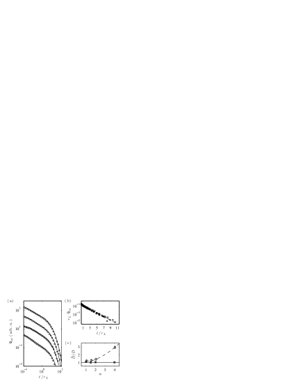
Figure 5: (a) Four simulated RTDs for molecules with rectangular shapes: $L_{\rm s}=5$, $L_{\rm l}=\alpha L_{\rm s}$, with $\alpha=1.0$ ($\lhd$), 1.5 ($\diamond$), 2.0 ($\square$), and 4.0 ($\circ$). Curves were vertically shifted for better visibility. The solid lines are best fits of Eq. (5) to the data after determination of $\tilde{D}$. (b) Exponential decay of $\Psi_{\rm rec}$ in the long-time regime and least square fits (dashed lines) for determining $\tilde{D}$. (c) $\tilde{D}/D$ as a function of the aspect ratio $\alpha=L_{\rm l}/L_{\rm s}$. Squares refer to fitting with Eq. (6), and circles to fitting with Eq. (2), with $R$ taken the gyration radius.

To a good approximation, the overall behavior can also be accounted for by using the solution Eq. (1) for circular-shaped molecules with an effective radius $R_{\rm mod}$. This is obtained by comparing the long-time limits in Eqs. (2) and (6), yielding

$$R_{\rm{mod}}=\frac{x_{1}}{\pi}\left(L_{\rm{l}}^{-2}+L_{\rm{s}}^{-2}\right)^{-1/2}\,.$$ (7)

The corresponding function gives a fit line in Fig. 5(a), which by the eye cannot be distinguished from the solid one shown. This finding will become useful later when discussing rotational effects in Sec. V and extensions of the theoretical treatment in Sec. VI.

V Additional rotational diffusion

For non-circular shapes of molecules, rotational effects can affect the RTD and hamper an accurate determination of translational diffusion coefficients, as described in the previous sections. On the other hand, one may utilize the modifications of the RTD to quantify rotational dynamics. To get insight in these effects, we consider here a simple model of discrete rotational moves that occur independent of translational moves (no rotation-translation coupling). In this model, rectangular-shaped molecules with aspect ratio $\alpha$, as considered in Sec. IV, perform transitions between $n$ possible orientations separated by an angle $\Delta_{\varphi}=2\pi/n$. The transitions occur between neighboring orientations around the molecule center with a constant rate $w_{\varphi}=D_{\varphi}/2\Delta_{\varphi}^{2}$, where $D_{\varphi}$ is the rotational diffusion coefficient. In the following we use $n=10$, i.e. $\Delta_{\varphi}=\pi/5$ and molecules of size $10\times 5$ in all simulations.

We first study only rotational movements of a single molecule at a fixed distance $r$ from the tip. For the analysis of this situation, it is convenient to consider the equivalent problem of a fixed molecule center and a tip performing jumps of size $r\Delta_{\varphi}$ on a concentric circle around the center. Clearly, if $r<r_{\rm min}\equiv L_{\rm s}/2$ [see inner circle in Fig. 6(a)], the signal is always “on”, while for $r>r_{\rm max}\equiv(L_{\rm s}^{2}+L_{\rm l}^{2})^{1/2}/2$ [see outer circle in Fig. 6(a)], the signal is always “off”.

In the regime $r_{\rm min}<r<r_{\rm max}$, a signal alternating between “on” and “off” states can be obtained. To derive the RTD $\Psi_{\rm rot}(t|r)$ for a given $r$ in this regime, we note that the “on”-periods correspond to time intervals, where the tip is located on certain arcs of the concentric circle with radius $r$. As sketched in Fig. 6(b), two opposing arcs of equal length are present if $r<L_{\rm l}/2$ (and $r>r_{\rm min}$), while for $r>L_{\rm l}/2$ (and $r<r_{\rm max}$), four equivalent arcs close to the corners of the rectangle appear. In analogy to the detection areas considered before for the translational diffusion, the arcs form detection lines with length $l_{r}$ given by

$$l_{r}=\left\{\begin{array}[]{ll}2\,r\,\mathrm{asin}\left(\frac{L_{\rm{s}}}{2r}\right)\,,&r_{\rm min}<r\leq\frac{L_{\rm l}}{2}\,,\\[4.30554pt] r\left[\mathrm{asin}\left(\frac{L_{\rm{s}}}{2r}\right)-\mathrm{acos}\left(\frac{L_{\rm{l}}}{2r}\right)\right]\,,&\frac{L_{\rm l}}{2}<r<r_{\rm max}\,.\end{array}\right.$$ (8)

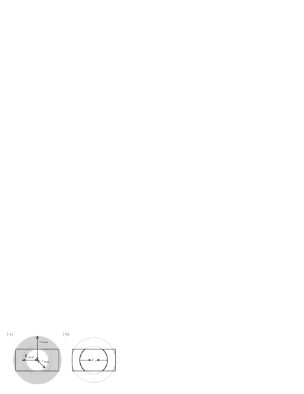
Figure 6: (a) Classification of distances between the molecule center (center of figure) and probe tip: In the circular blank core area, rational moves cannot influence the signal, while in the shaded area rotational moves are relevant. The dotted line marks the circle with radius $R_{\rm mod}$ assigned to the rectangle [cf. Eq. (7)]. (b) Origin of detection lines in the case of pure rotational diffusion: If the center of a rectangular molecule sets the origin of a co-rotating coordinate frame, rotational diffusion leads the (tip) probe to diffuse along concentric circles (thin lines). The intersection set of these circles with the rectangle yields arcs that define detection lines of length $l_{r}$ (bold lines).

For jump lengths $r\Delta_{\varphi}$ much smaller than $l_{r}$, we can, for calculating the RTD, consider the problem of a diffusing tip on a line of length $l_{r}$ with absorbing boundaries. The initial distribution is concentrated on two points at distance $r\Delta_{\varphi}$ from the boundaries. After determining the respective one-dimensional diffusion propagator $p(x,t)$, the first passage time distribution $\Psi_{\rm rot}(t|r)$ follows from $\Psi_{\rm rot}(t|r)=-\partial_{t}\int_{0}^{l_{r}}{\rm d}x\,p(x,t)$, yielding

$$\Psi_{\rm rot}(t|r)=\frac{4D_{\varphi}}{\pi}\displaystyle\sum_{n=0}^{\infty}\frac{q_{n}^{2}\sin\bigl{(}q_{n}\Delta_{\varphi})}{(2n+1)}\exp(-q_{n}^{2}D_{\varphi}t)\,,$$ (9)

where $q_{n}=q_{n}(r)=(2n+1)\pi r/l_{r}$. After averaging over the area of all positions between $r_{\rm{min}}$ and $r_{\rm{max}}$, taking into account that 2 equivalent arcs exist for $r_{\rm{min}}<r\leq L_{\rm l}/2$ and four equivalent arcs for $L_{\rm l}/2<r<r_{\rm{max}}$ the RTD

$$\Psi_{\rm{rot}}(t) =\mathcal{N}^{-1}\Biggl{[}\int_{r_{\rm{min}}}^{L_{\rm l}/2}\mathrm{d}r\,r\,\Psi_{\rm{rot}}(\mathbf{r},t)$$

$$\hskip 60.00009pt{}+2\int_{L_{\rm l}/2}^{r_{\rm{max}}}\mathrm{d}r\,r\,\Psi_{\rm{rot}}(\mathbf{r},t)\Biggr{]}$$ (10)

is obtained, where $\mathcal{N}=\pi(L_{\rm s}^{2}+L_{\rm l}^{2})/4$ is the normalization factor. To account for the effect of the finite jump length for detection lines with small length $l_{r}$, we had to deal with a rather complex situation with, among others, very small numbers of just 1-2 tip positions, whose precise location in turn depends on $r$ and $\Delta_{\varphi}$. After averaging over $r$ these effects of the discreteness of the jump length are, however, washed out.

In the presence of both rotational and translational diffusion, it is difficult to obtain exact analytical results for the RTD, because the problem cannot be described as a diffusion problem with a time-independent geometry of the absorbing boundary. Fortunately, in the situation, where rotational diffusion is relevant in the RTD, the results obtained for pure translation and pure rotation are sufficient to account for the overall behavior, as explained in the following.

The signal can turn from “on” to “off” due to rotational moves only if the molecule center is in the shaded area in Fig. 6(a). A typical arc in this area has an angle of about $\pi/4$ to $\pi/2$ [cf. Fig. 6(b)], which results in a typical time $\sim\tau_{\varphi}\equiv(\pi/4)^{2}/2D_{\varphi}$ for the molecule to leave the detection area by rotation. The typical time for a molecule center to traverse the shaded area in Fig. 6(a) is $\sim\tau_{\rm tr}\equiv(L_{\rm l}/2-L_{\rm s}/2)^{2}/4D=(\alpha-1)^{2}L_{\rm s}^{2}/16D$. Hence, if $\tau_{\varphi}\gg\tau_{\rm tr}$, the decay of the RTD should be governed by translational diffusion as described in Sec. IV. On the other hand, if $\tau_{\varphi}\ll\tau_{\rm tr}$, the rotational diffusion should become significant. It governs the RTD for short times $t\ll\tau_{\rm tr}$, while for $t\gtrsim\tau_{\rm tr}$ the dominant events are those, where the molecule center enters the “core area” $r\leq r_{\rm min}$ and leaves it by translational diffusion. Accordingly, the RTD becomes decomposable into one part given by pure rotational diffusion, i.e. Eq. (10), and a second part given by pure translational diffusion, i.e. Eq. (1) with $R=r_{\rm min}$.

Results of KMC simulations shown in Fig. 7 confirm these considerations. In this figure, representative RTDs in the presence of both rotational and translational diffusion are displayed for a rectangular molecule of size $10\times 5$ for various $D_{\varphi}/D$ ($=D_{\varphi}/Da^{2}$) ratios. For $D_{\varphi}/D=8\times 10^{-3}$ ($\tau_{\varphi}/\tau_{\rm tr}=25\gg 1$) rotational diffusion indeed has no influence, and the KMC data can be well described by Eq. (5) (dashed line). For $D_{\varphi}/D=2.8$ ($\tau_{\varphi}/\tau_{\rm tr}=0.07\ll 1$), a double shoulder characterizes the distribution. This reflects the separation into the two time regimes governed by rotational and translational diffusion, as demonstrated by the curves corresponding to Eq. (10) (solid line) and to Eq. (1) with $R=r_{\rm min}$ (dashed line). The relative weight of the two contributions was determined in the following way: By making the ansatz $\Psi(t)=B_{1}\Psi_{\rm rot}(t)+B_{2}\Psi_{\rm circ}(t)$, the coefficient $B_{2}$ was first determined by fitting $\Psi(t)\sim B_{2}\Psi_{\rm circ}(t)$ to the KMC data in the long-time regime [with $\Psi_{\rm circ}(t)$ taken from Eq. (2)]. Thereafter, the coefficient $B_{1}$ followed from the normalization of $\Psi(t)$. The small full symbols in Fig. 7 represent the distributions of residence times, during which the molecule center has entered the core area. These distributions are normalized to the overall fraction of the corresponding events. Their good agreement with the long-time behavior of the simulated data is a further proof that this regime is dominated by translational diffusion in the core area.

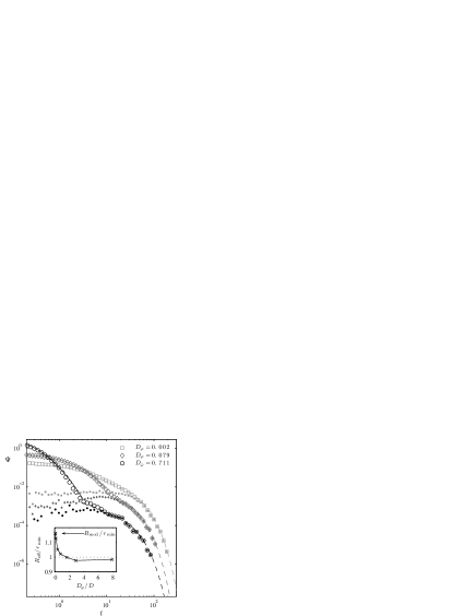
Figure 7: (a) Simulated RTDs for three different $D_{\varphi}$ (open symbols). Dashed lines correspond to Eq. (1) for translational diffusion with $R=R_{\rm eff}$ (see main text). Solid lines correspond to Eq. (10) for rotational diffusion. The small solid symbols refer to distributions of residence times, which belong to trajectories, where the molecule center has at least once entered the core area shown in Fig. 6(a). The inset shows the dependence of the effective radius $R_{\rm eff}$ on $D_{\varphi}/D$.

Generally, the influence of the rotational motion on the long-time regime can always be captured by defining an effective radius $R_{\rm eff}$, which follows from fitting the exponential decay in the long-time regime to Eq. (2). The behavior of this effective radius as a function of $D_{\varphi}/D$ is shown in the inset of Fig. 7. For $D_{\varphi}/D=0$ (no rotational diffusion), $R_{\rm eff}=R_{\rm mod}$, as discussed at the end of Sec. IV. With increasing $D_{\varphi}/D$, $R_{\rm eff}$ decreases and rapidly approaches $R_{\rm eff}=r_{\rm min}$. When $R_{\rm eff}=r_{\rm min}$, the rotational moves are so fast that, if a molecule center leaves the core area, the signal will almost immediately be turned off. The radii $R_{\rm eff}>r_{\rm min}$ for $D_{\varphi}/D\lesssim 1$ can be assigned to an effective circular detection area, which takes into account that a molecule center, when leaving the core area, typically diffuses over a certain effective distance before the signal is turned “off” because of a rotational move.

Let us finally address how our findings can be applied to extract rotational and translational diffusion coefficients if both types of molecular motion are present. As discussed above, if $\tau_{\varphi}\gg\tau_{\rm tr}$ [$D_{\varphi}/D\ll(L_{\rm l}/2-L_{\rm s}/2)^{-2}$] only translational diffusion coefficients can be determined from the RTD. When a double shoulder shows up in the RTD for $\tau_{\varphi}\lesssim\tau_{\rm tr}$ [$D_{\varphi}/D\gtrsim(L_{\rm l}/2-L_{\rm s}/2)^{-2}$], the rotational diffusion coefficient should also be determinable. In fact, using a Levenberg-Marquardt nonlinear fitting of Eq. (10) to the shoulder in the short-time regime, we obtain $\tilde{D}_{\varphi}=0.081$ for the diamonds and $\tilde{D}_{\varphi}=0.69$ for the circles, which agree well with the respective input values $D_{\varphi}=0.079$ and $D_{\varphi}=0.71$. Simultaneously, by fitting Eq. (2) to the shoulder in the long-time regime, $\tilde{D}$ values are determined. For this analysis, one can choose $R_{\rm eff}=r_{\rm min}$ first. If the resulting $\tilde{D}_{\varphi}/\tilde{D}$ turns out to be larger than one, $\tilde{D}$ should have a reliable value. However, if $\tilde{D}_{\varphi}/\tilde{D}\lesssim 1$, the $\tilde{D}$ value is underestimated because the effective radius $R_{\rm eff}$ is larger than $r_{\rm min}$. For our data in Fig. 7, we obtain $\tilde{D}=0.23$ (diamonds) and $\tilde{D}=0.25$ (circles), which in connection with the $\tilde{D}_{\varphi}$ values give $\tilde{D}_{\varphi}/\tilde{D}=0.36$ and $\tilde{D}_{\varphi}/\tilde{D}=2.76$, respectively. Indeed, $\tilde{D}$ for the circles agrees well with $D=1/4$, while $\tilde{D}$ for the diamonds is by 8% smaller.com In practice, it will generally be unlikely to encounter this deviation, because of the narrow regime $D_{\varphi}/D\lesssim 1$, where $R_{\rm eff}$ is larger then $r_{\rm min}$. If the problem is nevertheless present, the experimentalist may shift the $D_{\varphi}/D$ value to the favorable regime by changing the temperature.

VI Conclusions and discussion

Analysis of signal fluctuations from a locally fixed probe is a powerful means to determine diffusion coefficients. In this work we concentrated on the determination of diffusion coefficients of molecules on surfaces, but the concepts can also be useful in other fields such as, e.g., single-molecule fluorescence microscopy.Petrov and Schwille (2008); Zumofen et al. (2004)

The first focus of our treatment was on the implications of molecular shapes on the RTD. Since typical molecules used in experiments, as shown in Fig. 1, can have rectangle-like geometries $L_{\rm l}\times L_{\rm s}$ with aspect ratios $\alpha=L_{\rm l}/L_{\rm s}$ significantly larger than one, it was necessary to extend our former treatment, that was limited to molecules with a circular shape.Hahne et al. (2013) The exact solution Eq. (5) for such rectangular shapes was successfully applied to data obtained from KMC simulations, which served as surrogate for experimental results. It was shown that for $\alpha\gtrsim 1.5$, an application of the RTD for circular shapes, with $R$ taken as the gyration radius, yields erroneous results. However, when taking the modified radius defined in Eq. (7), the solution for circular shapes can also be used. It gives a very good approximation to the exact solution.

As discussed in the introduction, the RTD is the most favorable variant for analyzing the signal fluctuations, and we therefore focused our treatment to it here. Nevertheless, in some situations it may be helpful to analyze also the interpeak time distribution (ITD) or autocorrelation function (ACF). For the ACF, the consideration of shapes different from circular ones can be readily accounted for by defining corresponding detection functions, see Ref. Hahne et al., 2013.

For the interpeak times, on the other hand, we were not able to derive their distribution. One would need the diffusion propagator for the outer domain of an absorbing rectangle. A solution for this outer problem is difficult and we did not succeed to derive a closed form or to find a derivation in the literature. However, with the finding that the RTD for rectangular shapes can be well approximated by the RTD for circular shapes when introducing an appropriate radius, one can follow a corresponding route to find an approximate solution for the ITD. At long-times, the ITD is governed by exchange processes of different molecules, yielding an exponential decay with characteristic time $\propto d^{2}/D$, where $d$ is the mean intermolecular distance. For rectangular-shaped molecules, $d=(L_{\rm l}L_{\rm s}/\theta_{0})^{1/2}$, where $\theta_{0}$ is the coverage of the freely diffusing molecules. In practice, this coverage can be extracted from the signal as the ratio of the “on-periods” to the total observation time $T$, that is $\theta_{0}=\sum_{i}t_{i}/T$. For circular shapes, $d=(\pi R^{2}/\theta_{0})^{1/2}$. Comparing the corresponding characteristic times $d^{2}/D$, the effective radius

$$R_{\rm{cov}}=\left(\frac{L_{\rm l}L_{\rm s}}{\pi}\right)^{1/2}$$ (11)

is obtained. Inserting $R_{\rm{cov}}$ for $R$ in the exact solution for circular-shaped molecules [Eq. (10) in Ref. Hahne et al., 2013], one can check whether this provides a good approximation of the ITD of rectangular-shaped molecules. By comparison with data obtained from our KMC simulation, we indeed found good agreement.

The second focus of our treatment was on the implications of rotational diffusion on the RTD by considering as a first step a model of uncoupled rotation and translation. These implications become the more important the larger the aspect ratio is. For pure rotational diffusion, the analytical expression Eq. (10) was derived by considering diffusion along circular arcs, and by averaging over all possible tip-molecule distances. Combining this solution with the solution for pure translational diffusion, we succeeded to describe the behavior of the RTD when both rotational and translational diffusion are present. We showed, that when the ratio $D_{\varphi}/D$ of the rotational to the translational diffusion coefficient is larger than one, two shoulders appear in the RTD. From those, $D_{\varphi}$ and $D$ can be extracted separately. For $D_{\varphi}/D\lesssim 1$, an effective radius, varying between $r_{\rm min}=L_{\rm s}/2$ and $R_{\rm mod}$, needs to be taken into account. By employing KMC simulations we demonstrated how the theoretical approach can be applied.

Also for rotational diffusion we can discuss the implications on the ACF and ITD. In the case of the ACF, one can straightforwardly generalize (i) the detection functions for the angle degrees of freedom and (ii) the free diffusion propagator, which becomes simply the product of the free propagators for rotational and translational diffusion in the uncoupled case. The derivation of the behavior of the ITD can be done in close analogy to the RTD treatment. When deriving the part arising from pure rotation, one needs to replace the inner arcs [thick lines in Fig. 6(b)] with the outer arcs [thin lines in Fig. 6(b)]. Combining the corresponding solution with the approximate solution for pure translation (see discussion above), an effective radius now appears that varies between $R_{\rm{area}}$ (for $D_{\varphi}/D\to 0$) and $r_{\rm max}=[(L_{\rm l}/2)^{2}+(L_{\rm s}/2)^{2}]^{1/2}$ (for $D_{\varphi}/D\gtrsim 1$). Using the KMC simulations we again checked that this procedure gives good estimates for both diffusion coefficients $D_{\varphi}$ and $D$.

The model of uncoupled rotation and translation with a fixed jump angle $\Delta_{\varphi}$ is certainly a strong simplification and further work is necessary to account for non-uniform jump angles, rotation centers displaced from the molecule center, rotation-translation couplings, etc. Irrespective of these complications, the possibility to simultaneously determine rotational and translational diffusion coefficients is a promising perspective that calls for an experimental verification.