Automatic recognition and tagging of topologically different regimes in dynamical systems
Abstract.
Complex systems are commonly modeled using nonlinear dynamical systems. These models are often high-dimensional and chaotic. An important goal in studying physical systems through the lens of mathematical models is to determine when the system undergoes changes in qualitative behavior. A detailed description of the dynamics can be difficult or impossible to obtain for high-dimensional and chaotic systems. Therefore, a more sensible goal is to recognize and mark transitions of a system between qualitatively different regimes of behavior. In practice, one is interested in developing techniques for detection of such transitions from sparse observations, possibly contaminated by noise. In this paper we develop a framework to accurately tag different regimes of complex systems based on topological features. In particular, our framework works with a high degree of success in picking out a cyclically orbiting regime from a stationary equilibrium regime in high-dimensional stochastic dynamical systems.
1. Introduction
Critical transitions are abrupt changes in the behavior of nonlinear systems that arise after small changes in the parameters of a system. They are natural phenomenon which occur in across a vast range of spatial and temporal scales. Natural systems that exhibit sudden shifts in their behavior include the Earth’s climate, changes in ocean currents, large and sudden shifts in plant and animal populations, and the domino-like collapses observed in financial markets [25]. In a climatic example, data indicate that the Earth’s climate has swung between a “snowball Earth” and a “tropical” Earth numerous times in its history on a geologic time scale that is considered rapid [16]. Also on a global scale, an abrupt change in the strength and direction of the Gulf Stream as a result of climate change would prove catastrophic for the European climate [27]. Evidence suggests that such a change was partially responsible for the three-hundred year Little Ice Age in Europe beginning in the 17th century [18]. Ecology provides another good source of examples of catastrophic change; for instance, eutrophication of a lake occurs when nutrient-rich pollution reaches a critical threshold, at which point water clarity is suddenly and greatly reduced due to a bloom of algae, which in turn kills submerged flora [25, 24].
The aim of this paper is to develop robust methods by which to characterize and detect critical transitions between two or more regimes in the evolution of a dynamical systems. Formally, critical transitions as seen in natural system are associated to bifurcations in dynamical systems models. Bifucations occur when basins of attraction collide due to a small change in parameters, which can lead to the disappearance of one stable region and cause the stability of the system to undergo a sudden, or critical, transition. In models with stochasticity, bifurcations are particularly difficult to define, since the change in regime will depend on the particular realization of the underlying random variable. Some current approaches [5] use topological methods to devise sufficient conditions for bifurcations in stochastic dynamical systems, by using all possible realizations of the random variable. From a practical point of view, when the data generated by a system is acquired from a single, or a very limited number of realizations, such an approach may not be suitable. An additional challenge encountered in many real world systems is sparsity of, and noise pollution in, the available data. In this paper we outline a novel method to detect critical transitions in dynamical systems with additive noise or time series measured from real-world sources. Our approach is based on combining the theory of persistence homology with machine learning techniques.
The importance of detection and prediction of critical transitions from observational data in the context of ecology and climate science has been emphasized in a series of recent papers by Dakos, Ditlevsen, Scheffer [7, 8, 19, 20, 24, 25]. The main results of Scheffer, Dakos, and collaborators concern 1-dimensional time series in which a sequence of sliding windows is used to study changes in the statistical properties of the system over time. They demonstrate a correlation between the resilience of the systems under study and changes in the variance and autocorrelation measured across windows, especially in when the system is in close proximity to a bifurcation. A challenging aspect of their approach is the a priori lack of robustness of the statical methods involved since they rely on a number of choices of window size, detrending method, and visual interpretation of the results.
In this paper, we apply techniques from topological data analysis (TDA) to study, first, bifurcations in two classical dynamical systems with additive noise; and second, measurements of real-world, high-dimensional climate phenomena for which a critical transition manifests in the data. The main contribution of this work is the development of a methodology independent of dimension to detect the presence of a critical transitions. By studying the persistent homology of the point cloud data over windows (subsets) of a time series we can analyze and detect topologically distinct regimes of the behavior of the dynamical system. Another important feature of our approach is that it is robust, in the sense that data sets that are very close to one another yield topological objects that are also very close to one another, relative to some appropriate metric [6].
In the sections that follow, the paper is broken into two main parts. In Section 2 we summarize the relevant dynamical systems background as well as persistent homology, which allows the encoding of topological information in the form of persistence diagrams. In Section 3 we describe the basis for our classifier in the context of machine learning and the selection of relevant features from persistence diagrams, their relation to the underlying dynamical system, and the use of machine learning to classify a given system using the selected features. We focus on the case of periodic and quasi-periodic phenomena, and use degree 1 Betti numbers for detection of critical transitions. In Sections 4, we demonstrate the effectiveness of our algorithms in detecting bifurcations in noisy systems with conceptual computational models and follow this with analysis of real-world time series data. We conclude with a discussion of results and future directions in Section 5.
2. Background
2.1. Dynamical systems
We recall some basic facts about parameter-dependent differential equation, both deterministic and stochastic. Simple physical systems are often described by ordinary differential equations that depend explicitly on one or more parameters, of the form
| (1) |
where is a -function in all variables and the parameter space is a subset of . The corresponding flow, denoted depends in -fashion on time, initial condition and parameter, and satisfies
-
(i)
;
-
(ii)
, for all ,
where we denote by the diffeomorphism .
Two distinct flows and are called topologically conjugate if there exists a homeomorphism such that for all . The flows and are topologically equivalent if there exists a homeomorphism and a continuous time-rescaling function which is strictly increasing in such that for all . If the two flows are topologically equivalent, then maps the orbits of one flow onto the orbits of the other flow, preserving direction of time but not necessarily parametrization by time.
As the parameter of (1) varies, the topological equivalence between the flows for different values of may cease to exist. When this happens, we say that a bifurcation has occurred. The value of the parameter that marks the change of topology under variation of parameters is referred to as a bifurcation value. More precisely, is a bifurcation value if for any neighborhood of there is a parameter value such that and are not topologically equivalent.
Some bifurcations can be detected by analyzing the behavior of the flow in a small neighborhood of an equilibrium point; these are referred to as local bifurcations. Others require analyzing the whole phase portrait; those are referred to as global bifurcations. An example of a local bifurcation is the Hopf bifurcation, when a stable (unstable) equilibrium point becomes unstable (stable) and a stable (unstable) periodic orbit is born for some value of the parameter. An example of a global bifurcation is when a connecting orbit between two equilibrium points of saddle type breaks down for some value of the parameter. Global bifurcations can also more complicated sets, such as attractors, which can appear, disappear, merge into, or split from, one another. To recall, an attractor is a set invariant under the flow, for which there is a neighborhood of such that as for all .
Physical systems that are perturbed by external noise can be modeled by stochastic differential equations (SDE) which may also depend on parameters. Below, we detail the ways in which bifurcations in SDEs mirror those in ODEs. We consider the simplest type of SDE’s with additive Gaussian (white) noise
| (2) |
where is Gaussian noise with mean 0 and standard deviation 1, and is the noise intensity of the equation. This can be written as
| (3) |
where is a standard Brownian motion (that is, ). If is uniformly Lipschitz continuous, the equation (2) with initial condition has a solution that depends continuously on time, initial condition, and parameter. The dependence on time is only Hölder continuous. Moreover, the solution depends on the realization of the underlying Brownian motion. Another remark is that when the solution of the initial value problem for an SDE approaches uniformly the corresponding solution of the ODE (see [1, 12]).
Let be the space of continuous functions on reals, regarded as the path space of Brownian motions , equipped with the Wiener measure. More details can be found in Evans [12]. The probabilistic nature of SDEs forces a change in how one defines bifurcations. Briefly, the solutions of the stochastic differential equation (2) define what is known as a cocycle characterized by the following two properties:
-
(i)
for all ;
-
(ii)
, for all and all ,
where for . Here is the mapping . When reduces to a point, the cocycle property coincides with the usual flow property.
Two cocycles and are said to be topologically conjugate if there exists a family of homeomorphisms such that the mappings and are measurable for all , and the cocycles and are cohomologous, i.e., for all and almost all . A bifurcation value for (2) is a value such that for any neighborhood of there is such that is not topologically conjugate with . We notice that, unlike for flows, topological conjugacy of cocycles does not involve a time reparametrization. This is because in the stochastic case periodic orbits exist with zero probability. Additionally, we remark that the stochastic version of topological conjugacy requires an entire family of homeomorphisms to satisfy the measurability condition.
Crucially, in practice this definition is difficult to verify. One reason is that, when dealing with experimental data, it is not possible to generate a significantly large number of realizations of an experiment, but only a very limited number of them. In climate data, for example, only very few sets of proxy temperature measurements are available. In the subsequent sections, we will use topological tools to devise a practical method to characterize bifurcations in parameter-dependent SDEs. Instead of focusing on a single bifurcation value, we will examine a range of parameters and we will assess whether there is a significant change in the topological features of phase space over that range. In particular, we will look at attractors corresponding to different values of the parameter within the range, and we will characterize their topology in terms of the homology groups. Moreover, instead of looking at continuous solutions of ODEs, we will look at their time discretizations, so instead of paths, we will examine discrete sets of points.
2.2. Change of topology of attractors undergoing bifurcations
We consider the following specific situation. We start with the system (1) where the parameter space is some interval in . We assume that for some the system undergoes a bifurcation, and for the system has an attractor that depends on . Moreover, we assume that there is a change in the topology of the attractor, as follows. By we mean the singular homology of a topological space. Suppose that, for some we have:
In the above, in (iii), whether depends on the system. For a one dimensional system displaying hysteresis, the topology of the two attractors is indeed identical. On the other hand, in the case of a Hopf bifurcation, as in Section 4.1, the stable equilibrium point changes to a stable limit cycle meaning . The crucial observation is that near a bifurcation the homology of an attractor of the system changes due to the inherent instabilities of the system. However, computing the homology of an attractor is difficult. Instead, we will measure the change of topology of attractors via persistent homology, as explained below. Moreover, we will consider not only deterministic systems as described by (1) but also random dynamical systems, as described by (2).
2.3. From dynamical systems to point cloud data
We consider an ODE given by (1), or an SDE, given by (2), with sufficiently small. We consider the time evolution of a system, starting with some initial condition, and with the parameter slowly evolving. To the system output , we apply a time discretization with equal time increments that are sufficiently small. Thus, instead of a trajectory of the flow associated to (2), we consider an orbit of the -time map , where . Hence for all . We choose a real-valued test function and generate the time series . (For example, if are points in some Euclidean space , is the projection onto one of the coordinates.) We associate to this time series the delay coordinate vectors:
with is a sufficiently large embedding dimension and is a lag. Alternately, we can think of as a sliding window for the time series. On this set of delay-coordinate vectors we define a dynamical system given by the shift map
Thus, we represent the original dynamical system by a discrete dynamical system , whose phase space consists of delay coordinate vectors and the mapping is the shift map above.
First, consider the limit case when and (ODE with time-independent parameter). The Takens Embedding Theorem [26] and its extensions by Sauer, Yorke, Casdagli [23], imply that, for generic , and for small enough, there exists a sufficiently large such that on , , is conjugate to on some subset of delay coordinate vectors . In other words, the shift dynamics on delay coordinate vectors is an embedded copy of the original dynamics.
Now, if the parameter varies sufficiently slowly and the noise intensity is small enough, i.e., , are sufficiently small, sufficiently large -time interval, the dynamical system of follows closely a quasi-static attractor , for . The reconstructed dynamics provides an approximate copy of . The same assertion holds for , . Thus, the bifurcation in the deterministic system (1) will be reflected in (2) by the change in the topological features of the quasi-static, noisy attractors [5] in the interval . In what follows, we describe the topological tools that can be used to measure, in a robust way, the changes in the topology of these attractors in the neighborhood of a bifurcation.
We regard each delay coordinate vector (sliding windows) as an element of a point cloud data set, and we want to describe the topology of these point cloud data for all . We are interested in determining from changes in the topological features of these point cloud data whether the underlying system undergoes a bifurcation of the type described above.
2.4. From point cloud data to persistent topology
To each cloud point data as described in the previous section, we associate an algebraic representation of its topological features. The pipeline, shown schematically in (4), is the following: From the point cloud data one constructs a sequence, or filtration , of simplicial complex (Vietoris-Rips complex) which depends on a parameter (which can be thought of as the ‘resolution level’ for the data). The simplicial homology of each complex in is then computed. The key step of persistent homology is following the homology generators as the parameter varies. The output of this process is a diagram that summarizes the ‘birth’ and ‘death’ of homology generators; this diagram is referred to as a barcode or a persistence diagram.
| (4) |
We now provide some necessary background on homology to aid the reader in understanding the information contained in a persistence diagram. Homology is a classical technique for topological feature identification using linear algebra. A triangulated space gives rise to a vector space of chains: formal linear combinations of simplices. The geometric boundary gives rise to a linear boundary operator defined as ,
where by conventio means leaving the vertex out. The definition extends by linearity to the entire chain space. The -th homology quotient vector space . The -th Betti number is the rank of . The -st Betti number, which is the rank of , counts the number of 1-dimensional holes (‘tunnels’) in . Similarly counts the number of 2-dimensional holes (‘cavities’) in .
For a point cloud , the -Vietoris-Rips complex is a simplicial complex with vertices given by the points in , and a simplex included if and only if for all pairs of vertices. As grows, the Vietoris-Rips complex gains more simplices, producing a diagram of inclusions
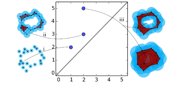
The technique of persistent homology introduced by [11] produces efficient algorithms to compute the homology of a diagram of spaces like this, summarizing it with a persistence diagram: a multiset of start and endpoints such that if is in the diagram, then there is a corresponding homology class that exists in all for . Long lifespans (eg., ) correspond to dominant topological features; short lifespans correspond to noise or small features. The coordinates and are termed birth and death times. (In this context, time refers solely to the monotone-increasing radius of the -balls used to construct the -Vietoris-Rips complex.)
For a classic overview of algebraic topology and homology, we recommend the book by [14]. For good overviews of persistent homology and its use in analyzing point clouds we recommend the survey articles by [13] or [4], or the books by [10] and [28]. For a general overview of computational topology see [17].
An example of persistent homology on a point cloud, and the corresponding persistence diagram is provided in Figure 2. The size of the blue disks centered on the black vertices corresponds to : Moving clockwise, the radii increase in size, beginning in the lower left corner, which yields a nested sequence of VR complexes. At a radius of , a small circle is born, which subsequently dies at . The feature is recorded by the point at , with the curve connecting the feature to its representation on the persistence diagram in the center. Another small feature exists for a single time step, indicated by line . Last, the large, central circle is also born at , but persists until it fills in at . This is shown in the two VR complexes on the right hand side and the curve . This final lifespan is significantly longer than the first two, implying that the corresponding feature is a dominant topological feature in the space.
2.5. From persistent topology to machine learning
The sequence of steps described above start with a sliding window along the time series and produce a topological summary encoded by a barcode. As the underlying system undergoes a bifurcation, the corresponding attractors experience topological changes that are reflected by barcode diagram changes. We want to be able to distinguish significant changes in the barcodes that can be used as indicators of bifurcations. For this purpose we use machine learning techniques.
Machine learning aims to reconstruct, or learning, a discrete (classification) or continuous (regression) function on some space given samples drawn from a distribution on that space. A rich toolbox has been developed to learn functions in various cases. In this paper we focus on using classifiers – our goal is to learn a discrete classification on the time series data under study.
Classifiers for discrete data can be linear or non-linear, depending on whether they can be modeled with a linear hyperplane as a decision boundary (delimiting the regions of input values that produce different results) or not. Furthermore, learning methods can be unsupervised, semi-supervised or supervised. For a supervised problem, sample points are drawn together with their expected values, and the system learns to generalize from seen examples to unseen examples: one example is linear regression or interpolation type problems. An unsupervised problem expects the machine learning algorithm to create some set of labels on its own: a typical example is most clustering algorithms in widespread use. For a detailed overview of machine learning topics we refer to the excellent textbook by Bishop [3].
3. Learning topological differences
A periodic or quasiperiodic multi-dimensional dynamical system under the influence of noise will tend to trace out a space with non-trivial degree 1 homology. The easiest example is given by the simple periodicity found in, e.g., the -plane of a simple pendulum: the periodic regime traces out a simple closed curve in the phase space of the system. A simple pendulum driven by a periodic force of sufficiently irrational period traces out the surface of a torus in . In these examples and in more general cases, the presence of a non-trivial degree 1 homology group in the point cloud traced out by a time series measurement of the system can be correlated to the presence and type of periodicity exhibited in the system.
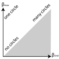
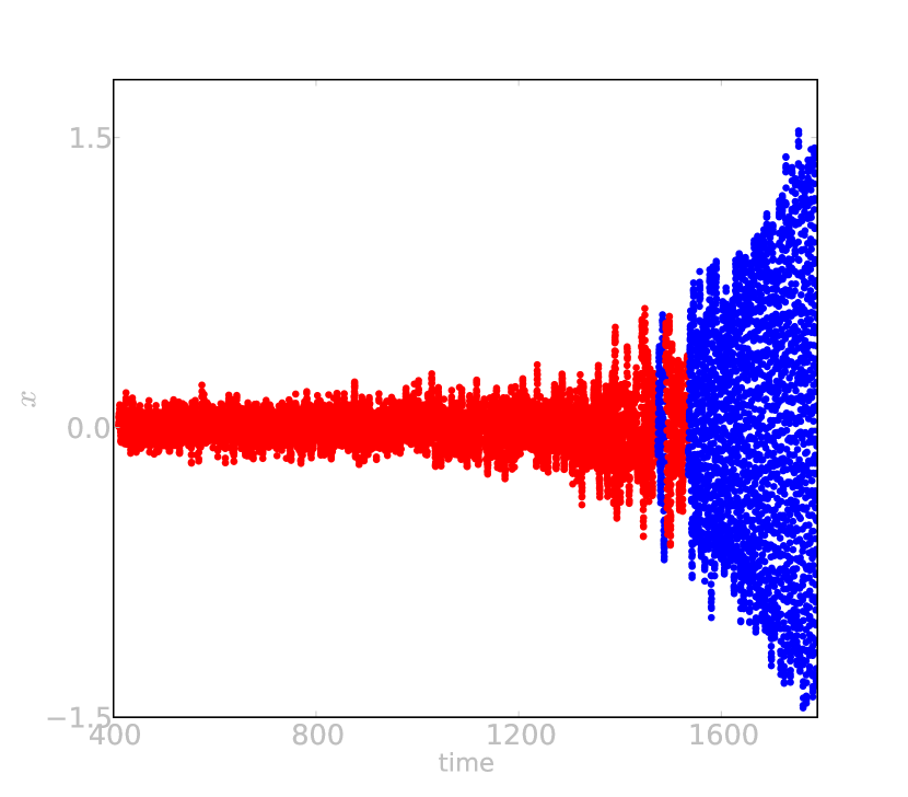
We aim to build a classifier capable of detecting the presence of highly significant 1-dimensional homology classes. Examples of features that we expect to easily discern are seen in Figure 3(c): the stationary parameter region of the system produces no significant persistent cycles, while the periodic regime produces a highly significant 1-cycle. We will accomplish this by training our classifier on the top persistence lengths of dimension 1 persistent homology. As described in the schematic in Figure 1, a high value for the most persistent Betti number and a low value for the second most persistent Betti number is an indication of periodic or quasi-periodic behavior, while several high values in the top most persistent Betti numbers indicated a more complex recurrent behavior.
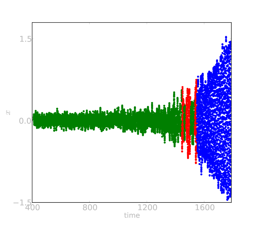
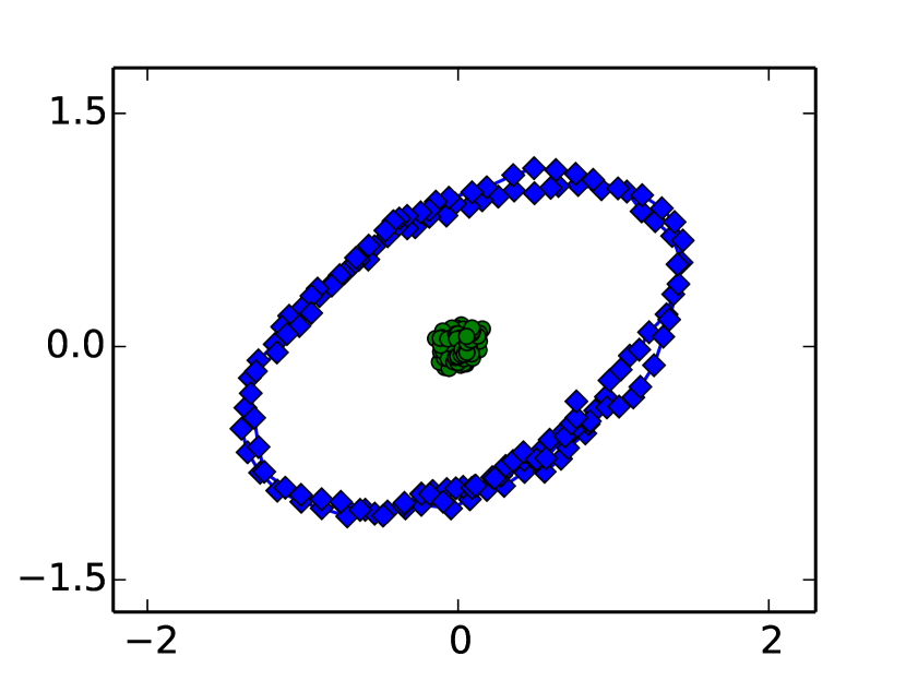
After (green diamonds)
For most practical computations, we pick an upper limit for the computation – any features that still exist when the computation terminates are assigned a death time after the upper limit time . Since the computation stops at , the computed persistences will not be able to distinguish further between bars after this point. We choose an and assign all such infinite bars a stopping value of , to avoid problems with infinite values in the machine learning algorithms. (For all experiments reported herein we chose .) We expect to distinguish features with very short persistence intervals from features with one or several highly persistent features. Highly persistent but finite bars and infinite bars are both indications of the presence of a significant topological feature.
To recognize periodic regimes, we use the two longest bars of the persistence barcode as features. Intuitively, a barcode for which the longest bar is significantly longer than the next longest bar is more similar to a circle, thus more likely to indicate a timeseries window from a periodic regime. In order to avoid arbitrary choices as much as possible, we use an unsupervised learning approach on the ordered pairs of lengths of features.
For recurrent or quasi-periodic regimes, we introduce more persistence features, in order to distinguish between possible intermediate regimes. For instance, in the case of the Lorenz attractor, certain parameter values yield a two-lobed attractor. With this heuristic, we expect to be able to distinguish (quasi-)periodicity around a single center from the two-lobe case which is qualitatively a different regime.
To tag a timeseries from a dynamical system with minimal operator intervention, we can use this persistence-based feature collection as the basis for a linear unsupervised learning system. There is a wealth of machine learning schemes to choose from – for simplicity, we work with -means clustering. Expecting few dominant features, we train classifiers on the top 2 or top 3 most persistent bar lengths. Our rationale for this was that assigning a hypothetical label of “high persistence”, “medium persistence” or “low persistence” to each of the top three values would produce exactly 10 possible ordered sequences of 3 labels. In practice, the tagging regimes tend to stabilize for our examples above 3 labels.
We imagine that if the analysis calls for it, a different unsupervised or semi-supervised method may well be used; semi-supervised methods requiring more effort to tag the supervision part of data input. For our test cases, however, already -means performed well beyond our expectations – see Section 4 for details – and we save the exploration of available machine learning methods for future work.
An important detail that we note is that we fully expect these methods to break down once the periodicity length significantly exceeds the window size.
4. Results
We demonstrate the effectiveness of the persistence-based automatic tagging algorithm on three experiments. First, we analyze a non-chaotic, stochastic system , which undergoes a local Hopf bifurcation. Second, we explore the detection of global bifurcations in a chaotic system, namely the Lorenz attractor. We vary the parameter through a global bifurcation, from to [9]. Lastly, we investigate temperature and CO2 records obtained from the Vostok ice core [22]
4.1. Hopf bifurcation
There are many systems that exhibit a Hopf bifurcation. Without loss of generality, we may consider the following stochastic system,
| (5) | ||||
| (6) |
where represent noise level and and are one-dimensional Weiner processes [15]. This system, with and and varying linearly with time , for small, is a classic model of biological oscillators. A realization is plotted in Figure 3. We note that the corresponding deterministic system () with time-independent parameter () undergoes a Hopf bifurcation for .
As we vary the parameter , the system progresses from a noisy but stationary regime to a periodic regime, tracing out widening circles in the -–plane. In [2], Berwald and Gidea use these topological changes in conjunction with distance metrics on persistent homology bar codes on similar point cloud windows to detect changes in the trajectory as drifts in time. In the current manuscript, we take take this a step further by applying the unsupervised learning tools described above to cluster the data windows in the time series. We illustrate the results for example windows from the two regimes in Figure 3. In Figure 3(a) we use 2-means clustering, and the learning algorithm is confident in locating the bifurcation in terms of the growth of the orbit, only faltering when stochastic effects cause the cycle radius to decrease for a short period of time around . In Figure 3(b), by using the same region that caused an issue in Figure 3(a) is highlighted by the intermediate cluster. One of the strengths of our method is its ability to highlight regions of uncertainly in the data. In this case, the level of noise contributes to uncertainty as the bifurcation grows into a limit cycle, which is exactly the region that we would like our algorithms to locate.
4.2. Lorenz equations
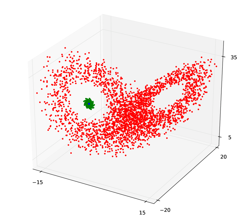
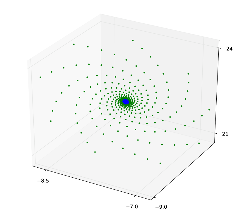
The Lorenz equations have a long history of study in dynamical systems and provide a fruitful test bed. The equations were derived by Edward Lorenz in the 1960s and represent a simplified model of atmospheric convection. Serendipitously, Lorenz discovered that they exhibit sensitivity to initial conditions, a finding which launched decades of research into chaotic attractors. The equations are defined by:
| (7) | ||||
| (8) | ||||
| (9) |
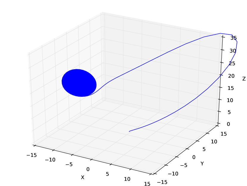
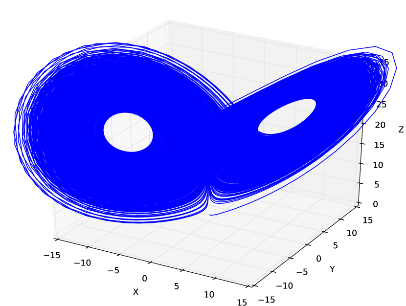
where are real-valued parameters. We fix and , their “classic” values. We change so as to reorganize the unstable manifold. In particular, when we observe a trajectory that approaches one of two stable fixed points for initial conditions different from (0,0,0). Alternatively, when , the trajectory organizes itself on a stable manifold that resembles closely the classic “butterfly wings” of the Lorenz attractor at the classic value of . (The choice of was inconsequential to the topological conclusions of the tagging algorithms – we could have very well chosen .)
A trajectory for is shown in Figure 4(a). The trajectory and asymptotic behavior depend on the initial condition. The dependence exhibits an important and well-known symmetry, manifesting as a rotation by about the axis,
There is another attractor, symmetric to the one in Figure 4(a), and w.l.o.g. we can focus on just one of the two attractors in our experiments. For , the situation is the same, except that in this case, the attractor consists of the two lobes plotted in Figure 4(b).
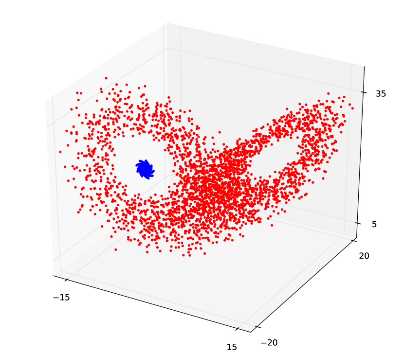
It is this global difference which is clear from a topological perspective as well. After first removing a transient from the trajectory we apply the heuristics detailed in Section 3 to distinguish the two parameter regimes in an unsupervised manner. The phase space is three-dimensional and we take as input point clouds composed of windows of time series. We train a single unsupervised classifier on windows from both values of , and use the trained classifier to tag windows from the two time series.
The result is a clean separation of the data, as shown in Figure 5. For instance, with , the data is partitioned into two classes according to the value of . Increasing does little to improve the partitioning, while it does identify the central region near the fixed point as separate from the earlier part of the trajectory. In Figure 5(c) we highlight the two classes identified for central spiral, , seen in Figure 5(b). One way to interpret these results is that quasiperiodic behavior occurring below a certain spatial resolution is singled out as a third class in this case.
4.3. Vostok temperature and \ceCO2 data
Ice cores offers a unique window into past climates on Earth. One of the longest obtained is from the Vostok research station in Antarctica. From this and other ice cores it is possible to reconstruct various aspects of Earth’s climate and atmosphere over 400 000 years into the past. Two measurements possible to obtain from an ice core are atmospheric \ceCO2 concentration and atmospheric temperature (often through a proxy such as an oxygen isotope ratio).
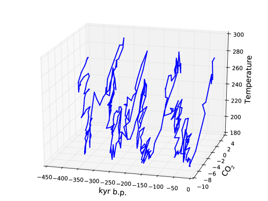
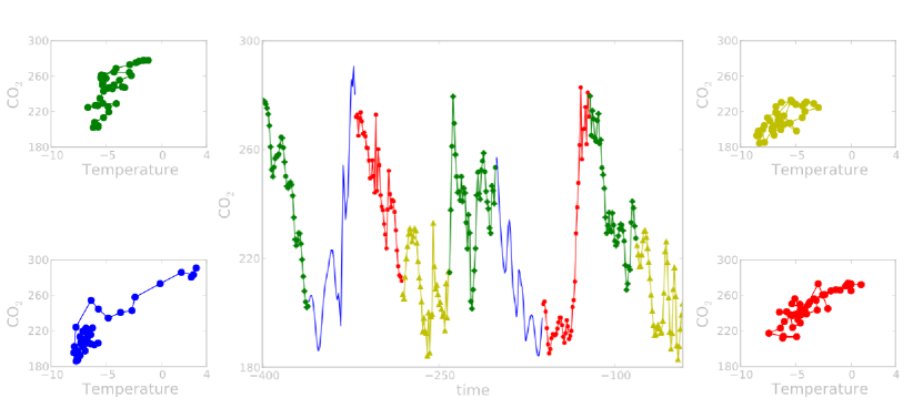
In the case of \ceCO2 and temperature, there is a lag in which rising temperatures actually precede a rise in \ceCO2. When plotted in three dimensions, these lags are observable as small-radius spiral in the time series, as seen in Figure 6. These lags are a poorly understood aspect of climate change in the geologic record.
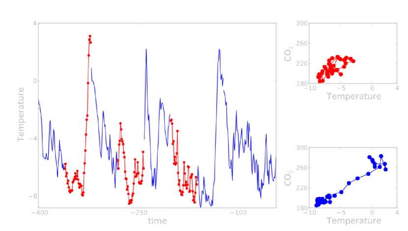
By analyzing the temperature – \ceCO2 data windows of length in two-dimensions, we can distinguish regimes in the climate record using our algorithms. Combining the time record with the tagging of windows yields the classifications shown in Figures 7 and 8. For values of it is possible to distinguish regimes similar to those found in Dakos, et al. [7]. In particular, we find the added granularity of a higher number of clusters important to separate the marginally more stationary regimes, yellow ’s, which correspond to regions of “critical slowing down” in Dakos, et al., from regimes that possess small loops but also a definite linear trend. Finer granularity in the data, which would enable a shorter window size, would likely aid in the analysis in this case. As in other work, especially [7], the sparsity of the data can be a hindrance to exacting analysis.
The value of an analysis like this is similar to the analysis exhibited for breast cancer in [21]: we are able to recognize a known distinct regime in the Vostok data set – and also several other regimes that recur in the data set with internal homogeneity. The topological and machine learning based perspective emerges as a way to highlight known, as well as possible new, patterns in the data.
5. Conclusion
We have demonstrated that combining persistence barcode lengths as features with an unsupervised machine learning protocol produces strong results in dynamical systems models exhibiting both global and local bifurcations and in automatically recognizing and tagging different regimes for time series from dynamical systems. The topological feature selection is robust to noise and gives a powerful predictor for bifurcation values in noisy system when many realizations may be computationally difficult. In Section 4.1, by tagging distinct regimes based on recurrent behavior, the classification scheme is able to handle the uncertainty of introduced by the noise by assigning the majority of that region a separate class.
We show also that global bifurcations, from stable to chaotic regimes for instance, can be detected in an unsupervised manner in Section 4.2. In this case we are concerned with the topological changes in the stable manifold, which are large enough so that we focus solely on the deterministic system. We showed that the classification for such a bifurcation is extremely precise, with no overlap in the two regimes. Extending results from Section 4.1 to a more general case, stochastic version of the Lorenz equations is part of ongoing research.
Furthermore, the approach using computational topology as feature selection and machine learning techniques for unsupervised classification has proven to produce interesting results on real world data sets. We showed that learning algorithms are able to distinguish regimes have previously been distinguished statistically by Dakos, et al.. In addition, by choosing different numbers of clusters, we are able to partition the data based on topological similarity. While this does not directly answer certain geological questions concerning temperature or \ceCO2 in this case, identifying new and distinct regimes is important its own right.
Acknowledgements
JJB would like to thank Dr. Richard McGehee for providing the Vostok ice core data.
References
- [1] L. Arnold “Random Dynamical Systems” Berlin: Springer, 1998
- [2] Jesse Berwald and Marian Gidea “Critical Transitions In a Model of a Genetic Regulatory System” In arXiv, 2013
- [3] Christopher M. Bishop “Pattern recognition and machine learning” Springer, 2006
- [4] G. Carlsson “Topology and data” In American Mathematical Society 46.2, 2009, pp. 255–308
- [5] Xiaopeng Chen, Jinqiao Duan and Xinchu Fu “A sufficient condition for bifurcation in random dynamical systems” In Proc. Amer. Math. Soc., 2010, pp. 965–973
- [6] David Cohen-Steiner and Herbert Edelsbrunner “Stability of persistence diagrams” In Discrete and Computational Geometry 37.1, 2007, pp. 103–120 URL: http://www.springerlink.com/index/F51R061K4X3X6U54.pdf
- [7] Vasilis Dakos et al. “Slowing down as an early warning signal for abrupt climate change.” In Proceedings of the National Academy of Sciences of the United States of America 105.38, 2008, pp. 14308–12 DOI: 10.1073/pnas.0802430105
- [8] Peter D. Ditlevsen and Sigfus J. Johnsen “Tipping points: Early warning and wishful thinking” In Geophysical Research Letters 37.19, 2010, pp. 2–5 DOI: 10.1029/2010GL044486
- [9] Eusebius J Doedel, Bernd Krauskopf and Hinke M Osinga “Global bifurcations of the Lorenz manifold” In Nonlinearity 19.12, 2006, pp. 2947–2972 DOI: 10.1088/0951-7715/19/12/013
- [10] H. Edelsbrunner and J. Harer “Computational Topology: an Introduction” AMS Press, 2009
- [11] H. Edelsbrunner, D. Letscher and A. Zomorodian “Topological persistence and simplification” In Discrete and Computational Geometry 28.4, 2002, pp. 511–533
- [12] Lawrence C. Evans “An Introduction to Stochastic Differential Equations” American Mathematical Society, 2013
- [13] R. Ghrist “Barcodes: the persistent topology of data” In Bulletin of the American Mathematical Society 45.1, 2008, pp. 61 –75
- [14] A. Hatcher “Algebraic topology” Cambridge University Press, 2002
- [15] Desmond J Higham “An Algorithmic Introduction to Numerical Simulation of Stochastic Differential Equations” In SIAM review 3.22, 2001, pp. 4863–4869 DOI: 10.1039/b104835j
- [16] P. F. Hoffman “A Neoproterozoic Snowball Earth” In Science 281.5381, 1998, pp. 1342–1346 DOI: 10.1126/science.281.5381.1342
- [17] Tomasz Kaczynski, Konstantin Mischaikow and Marian Mrozek “Computational Homology” Springer, 2004
- [18] L.D. Keigwin “The Little Ice Age and Medieval Warm Period in the Sargasso Sea” In Science (New York, N.Y.) 274.5292, 1996, pp. 1503–8
- [19] Timothy M Lenton et al. “Tipping elements in the Earth’s climate system.” In Proceedings of the National Academy of Sciences of the United States of America 105.6, 2008, pp. 1786–93 DOI: 10.1073/pnas.0705414105
- [20] V. N. Livina and T. M. Lenton “A modified method for detecting incipient bifurcations in a dynamical system” In Geophysical Research Letters 34.3, 2007, pp. 1–5 DOI: 10.1029/2006GL028672
- [21] P. Y. Lum et al. “Extracting insights from the shape of complex data using topology” In Scientific Reports 3, 2013 DOI: 10.1038/srep01236
- [22] Eric Monnin et al. “Atmospheric CO2 Concentrations Over the Last Glacial Termination” In Science 291, 2001, pp. 112–114
- [23] Tim Sauer, James A Yorke and Martin Casdagli “Embedology” In Journal of Statistical Physics 65.3 Springer, 1991, pp. 579–616
- [24] Marten Scheffer et al. “Catastrophic shifts in ecosystems.” In Nature 413.6856 Nature Publishing Group, 2001, pp. 591–6 DOI: 10.1038/35098000
- [25] Marten Scheffer et al. “Early-warning signals for critical transitions” In Nature 461.7260 Nature Publishing Group, 2009, pp. 53–59 DOI: 10.1038/nature08227
- [26] F Takens “Detecting strange attractors in turbulence” In Dynamical systems and turbulence, Warwick 1980 Springer, 1981, pp. 366–381 URL: http://www.springerlink.com/index/b254x77553874745.pdf
- [27] Michael Vellinga and Richard A. Wood “Global Climatic Impacts of a Collapse of the Atlantic Thermohaline Circulation” In Climate Change 54, 2002, pp. 251–267 DOI: 10.1029/94JC00522
- [28] A.J. Zomorodian “Topology for computing” Cambridge Univ Pr, 2005