Summing Large-N Towers in Colour Flow Evolution

Abstract

We consider soft gluon evolution in the colour flow basis. We give explicit expressions for the colour structure of the (one-loop) soft anomalous dimension matrix for an arbitrary number of partons, and show how the successive exponentiation of classes of large-$N$ contributions can be achieved to provide a systematic expansion of the evolution in terms of colour supressed contributions.

1 Introduction

In order to reliably interpret current and upcoming measurements at the LHC, precise QCD predictions for multi-jet final states are indispensable. These include both fixed-order calculations, as well as their combination with analytic resummation and/or parton shower event generators, e.g. Sjostrand:2007gs ; Bahr:2008pv ; Gleisberg:2003xi , to sum leading contributions of QCD corrections to all orders, such as to arrive at a realistic final state modelling. Fixed-order calculations at leading and next-to-leading order in the strong coupling are by now highly automated, and frameworks to automatically resum a large class of observables have been pioneered as well Banfi:2003je . The combination of NLO QCD corrections with event generators Frixione:2002ik ; Nason:2004rx ; Nagy:2005aa ; Platzer:2011bc ; Hoeche:2011fd ; Hartgring:2013jma is an established research area, and first steps towards combining analytic resummation and event generators have been undertaken Alioli:2012fc .

The efficient treatment of QCD colour structures is central to both fixed-order and resummed perturbation theory. Particularly the use of the colour flow basis has led to tremendously efficient implementations of tree-level amplitudes Maltoni:2002mq ; Duhr:2006iq ; Gleisberg:2008fv , which can be used both for leading order calculations, as well as one-loop corrections within the context of recent methods requiring only loop integrand evaluation (see Reuschle:2013qna for the exact treatment of the colour flow basis in the one-loop case). This colour basis is closely linked to determining initial conditions for parton showering. After evolving a partonic system through successive parton shower emissions, while keeping track of the colour structures (in the large-$N$ limit), colour flows also constitute the initial condition to hadronization models; this includes the dynamics of how multiple partonic scatterings are linked to hadronization. Colour reconnection models, such as those described in Sandhoff:2005jh ; Gieseke:2012ft , are exchanging colour between primordial hadronic configurations like strings or clusters, and have proven to be of utmost phenomenological relevance in the description of minimum bias and underlying event data.

Despite its relevance to event generators, the colour flow basis has typically not been considered in analytic resummation, most probably for the reason of being not the most simple or minimal basis. While recent work has focused on obtaining minimal (and even orthogonal) colour bases Keppeler:2012ih , an intuitive connection to the physical picture is hard to maintain in such approaches. It is until now an open question, whether amplitudes can be evaluated in a similarly efficient way in such bases. Also, in analytic resummation, a matching to a fixed-order calculation is usually mandatory and the use of colour flow bases could allow to use the full power of automated matrix element generators within this context. Understanding soft gluon evolution in the colour flow basis thus seems to be a highly relevant problem to address, which can also shed light on colour reconnection models, being so far based on rather simple phenomenological reasoning.

The purpose of the present work is to study soft gluon evolution in the colour flow basis. While for a fixed, small number of partons the exponentiation of the soft gluon anomalous dimension matrix can be performed either analytically or numerically, the case for a large number of partons is rapidly becoming intractable. This limitation thus prevents insight into the soft gluon dynamics of high-multiplicity systems relevant to both improved parton
shower algorithms Schofield:2011zi ; Platzer:2012qg as well as colour reconnection models. We will derive the general structure of the soft anomalous dimension matrix in the colour flow basis for an arbitrary number of partons, and tackle its exponentiation by successive summation of large-$N$ powers in a regime where the kinematic coefficients $\gamma$ are of comparable size to the inverse of the number of colours, $\gamma N\sim 1$, leading to a computationally much more simple problem than the full exponentiation. This strategy can well be applied to a large number of partons in an efficient way.

This paper is organized as follows: In section 2 we set our notation and present the general form of the soft gluon anomalous dimension. In section 3 we derive its exponentiation and show how subsequent towers of large-$N$ contributions can be summed in a systematic way. Section 4 is devoted to a few numerical studies of testing the accuracy of these approximations in a simple setting of QCD $2\to 2$ scattering, while section 5 presents an outlook on possible future applications before arriving at conclusions in section 6. A number of appendices is devoted to calculational details and for reference formulae to achieve what we will later call a next-to-next-to-next-to-leading colour (N³LC) resummation.

2 Notation and Soft Anomalous Dimensions

We consider the soft-gluon evolution of an amplitude $|{\cal M}_{n}\rangle$ involving $n$ coloured legs, either in the fundamental or adjoint representation of $\text{SU}(N)$, with in general $N$ colour charges. The amplitude is a vector in both colour and spin space, though we shall here mainly be interested in the colour structure, decomposing the amplitude into a colour basis $\{|\sigma\rangle\}$,

$$|{\cal M}_{n}\rangle=\sum_{\sigma}{\cal M}_{n,\sigma}|\sigma\rangle\ .$$ (1)

We assume that all momenta of the amplitude are taken to be outgoing, and will order the fundamental and adjoint representation legs successively as

$$\alpha=1_{{\mathbf{N}}},2_{\bar{{\mathbf{N}}}},...,(n_{q}-1)_{{\mathbf{N}}},n_{q,\bar{{\mathbf{N}}}},(n_{q}+1)_{{\mathbf{A}}},...,(n_{q}+n_{g})_{{\mathbf{A}}}$$

for the case of $n_{q}$ fundamental and anti-fundamental, and $n_{g}$ adjoint representation legs. We will consider soft gluon evolution of the amplitude,

$$|{\cal M}^{\prime}_{n}\rangle=e^{\mathbf{\Gamma}}|{\cal M}_{n}\rangle\ ,$$ (2)

with the soft anomalous dimension

$${\mathbf{\Gamma}}=\sum_{\alpha\neq\beta}\Gamma^{\alpha\beta}\ {\mathbf{T}}_{\alpha}\cdot{\mathbf{T}}_{\beta}\ ,$$ (3)

in terms of the usual colour charge products ${\mathbf{T}}_{\alpha}\cdot{\mathbf{T}}_{\beta}$. Though sometimes basis independent results can be obtained for the soft gluon evolution, e.g. Forshaw:2008cq , one in general sticks to a particular basis of colour structures in order to obtain a matrix representation of ${\mathbf{\Gamma}}$ such that the exponentiation can be performed.

We shall here consider the colour flow basis, by translating all colour indices into indices transforming either in the fundamental (${\mathbf{N}}$) or the anti-fundamental ($\bar{{\mathbf{N}}}$) representation. For a thorough derivation of this paradigm, including a list of Feynman rules and their application to fixed-order calculation, see for example Maltoni:2002mq . Translating the labelling of physical legs, $\alpha$, to a labelling of corresponding colour and anti-colour ‘legs’,

$$k \leftrightarrow \alpha=k_{\mathbf{N}}$$

$$\overline{k-1} \leftrightarrow \alpha=k_{\bar{\mathbf{N}}}$$

$$\left.\begin{array}[]{c}\overline{k-n_{q}/2}\\ k-n_{q}/2\end{array}\right\} \leftrightarrow \alpha=k_{\mathbf{A}}$$ (6)

we are able to label the basis tensors in the colour flow basis by permutations of the anti-colour indices relative to the colour indices,

$$|\sigma\rangle=\left|\begin{array}[]{ccc}1&...&m\\ \sigma(1)&...&\sigma(m)\end{array}\right\rangle=\delta^{i_{1}}_{i_{\overline{\sigma(1)}}}\cdots\delta^{i_{m}}_{i_{\overline{\sigma(m)}}}\ ,$$ (7)

where $m=n_{q}/2+n_{g}$. A pictorial representation of these basis tensors is given in figure 1.

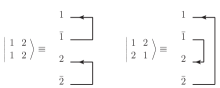
Figure 1: An illustration of the colour basis chosen for the case of two colour flows. Connected lines correspond to Kronecker-$\delta$ symbols in the space of (anti-)fundamental representation indices.

The colour charges (note that ${\mathbf{T}}_{\alpha}\cdot{\mathbf{T}}_{\beta}={\mathbf{T}}_{\beta}\cdot{\mathbf{T}}_{\alpha}$) translate as (obvious cases relating colour and anticolour are not shown):

$${\mathbf{T}}_{\alpha}\cdot{\mathbf{T}}_{\beta}={\mathbf{T}}_{k}\cdot{\mathbf{T}}_{l} \alpha=k_{\mathbf{N}},\beta=l_{\mathbf{N}}$$

$${\mathbf{T}}_{\alpha}\cdot{\mathbf{T}}_{\beta}={\mathbf{T}}_{k}\cdot{\mathbf{T}}_{\bar{l}} \alpha=k_{\mathbf{N}},\beta=(l+1)_{\bar{\mathbf{N}}}$$

$${\mathbf{T}}_{\alpha}\cdot{\mathbf{T}}_{\beta}={\mathbf{T}}_{k}\cdot{\mathbf{T}}_{\bar{l}}+{\mathbf{T}}_{k}\cdot{\mathbf{T}}_{l} \alpha=k_{\mathbf{N}},\beta=(l+n_{q}/2)_{\mathbf{A}}$$

$${\mathbf{T}}_{\alpha}\cdot{\mathbf{T}}_{\beta}={\mathbf{T}}_{k}\cdot{\mathbf{T}}_{\bar{l}}+{\mathbf{T}}_{k}\cdot{\mathbf{T}}_{l} \alpha=(k+n_{q}/2)_{\mathbf{A}},$$

$$+{\mathbf{T}}_{l}\cdot{\mathbf{T}}_{\bar{k}}+{\mathbf{T}}_{\bar{k}}\cdot{\mathbf{T}}_{\bar{l}} \beta=(l+n_{q}/2)_{\mathbf{A}}$$ (8)

and the colour flow charge products are expressed as

$${\mathbf{T}}_{i}\cdot{\mathbf{T}}_{j}=\frac{1}{2}\left(\delta^{i^{\prime}}_{j}\delta^{j^{\prime}}_{i}-\frac{1}{N}\delta^{i^{\prime}}_{i}\delta^{j^{\prime}}_{j}\right)$$ (9)

for a system of two ${\mathbf{N}}$ (and similarly for a system of two $\bar{{\mathbf{N}}}$) legs, and by

$${\mathbf{T}}_{i}\cdot{\mathbf{T}}_{\bar{j}}=-\frac{1}{2}\left(\delta^{i^{\prime}}{}_{\bar{j}^{\prime}}\delta^{\bar{j}}{}_{i}-\frac{1}{N}\delta^{i^{\prime}}{}_{i}\delta^{\bar{j}}{}_{\bar{j}^{\prime}}\right)$$ (10)

for a ${\mathbf{N}}\bar{{\mathbf{N}}}$ correlation. Hence the anomalous dimension reads

$${\mathbf{\Gamma}}=\sum_{i<j}(\gamma_{ij}{\mathbf{T}}_{i}\cdot{\mathbf{T}}_{j}+\gamma_{\bar{i}\bar{j}}{\mathbf{T}}_{\bar{i}}\cdot{\mathbf{T}}_{\bar{j}})+\sum_{i,j}\gamma_{i\bar{j}}{\mathbf{T}}_{i}\cdot{\mathbf{T}}_{\bar{j}}\ ,$$ (11)

where the form of the $\gamma$ can be inferred from eq. 8, e.g.

$$\gamma_{kl}=\Gamma^{\alpha\beta}+\Gamma^{\beta\alpha} \alpha=k_{\mathbf{N}},\beta=l_{\mathbf{N}}$$ (12)

$$\gamma_{k\bar{l}}=\Gamma^{\alpha\beta}+\Gamma^{\beta\alpha} \alpha=k_{\mathbf{N}},\beta=(l+1)_{\bar{\mathbf{N}}}$$

$$\gamma_{k\bar{k}}=0 \alpha=\beta=(k+n_{q}/2)_{\mathbf{A}}\ .$$

Examples of the non-diagonal part of the colour correlators are given in figure 2.

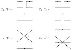
Figure 2: Illustration of the non-diagonal contributions to colour charge products acting on colour flow basis tensors. Note that the ‘singlet’ operators are entirely equivalent to the ‘swapping’ ones.

Since the colour flow charge products effectively describe one-gluon exchange between two colour flow lines, the general form of the matrix representation of ${\mathbf{\Gamma}}$ is straightforwardly found to be given by

$$[\tau|{\mathbf{\Gamma}}|\sigma]=\left(-N\Gamma_{\sigma}+\frac{1}{N}\rho\right)\delta_{\tau\sigma}+\Sigma_{\tau\sigma}\ ,$$ (13)

where

$$\Gamma_{\sigma}=\frac{1}{2}\sum_{i}\gamma_{i\overline{\sigma(i)}}\ ,$$ (14)

$$\rho=\frac{1}{2}\left(\sum_{i,j}\gamma_{i\bar{j}}-\sum_{i<j}(\gamma_{ij}+\gamma_{\bar{i}\bar{j}})\right)\ ,$$ (15)

while the off-diagonal elements are given by

$$\Sigma_{\tau\sigma}=\sum_{i,j}\Sigma_{ij\tau(i)\tau(j)}\delta_{\tau(i)\sigma(j)}\delta_{\tau(j)\sigma(i)}\prod_{k\neq i,j}\delta_{\tau(k)\sigma(k)}$$ (16)

with

$$\Sigma_{ijkl}=\frac{1}{2}(\gamma_{ij}+\gamma_{\bar{k}\bar{l}}-\gamma_{i\bar{k}}-\gamma_{j\bar{l}})\ ,$$ (17)

i.e. only non-vanishing when connecting two basis tensors which do not differ by more than a transposition in the permutation identifying these (note that the Kronecker $\delta$’s in eq. 16 ensure exactly one transposition between $\tau$ and $\sigma$ and the sum consists of solely one term).

3 Summation of Large-$N$ Towers

Though the exponentiation of the soft anomalous dimension matrix is possible either analytically or using standard numerical algorithms for a fixed (small) number of external legs, a general expression seems yet out of reach, due to the rapid growth of the dimension of colour space with the number of partons. In this section, we will consider successive approximations to the full exponentiation by subsequently summing towers of large-$N$ contributions, $\gamma^{n}N^{n-k}$. To derive the form of the large-$N$ towers, let us start from the structure of the soft anomalous dimension matrix,

$${\mathbf{\Gamma}}\equiv N\underline{\Gamma}+\underline{\Sigma}+\frac{1}{N}\rho\underline{1}\ ,$$ (18)

where we choose an arbitrary ordering of the permutations to identify these with the indices of the rows and columns of the matrix representation, such that $\underline{\Gamma}={\rm diag}(\{-\Gamma_{\sigma}\})$, and $\underline{\Sigma}=(\Sigma_{\rho\sigma})$ does not contain any diagonal elements.

The $n$-th power of the matrix representation then takes the form

$${\mathbf{\Gamma}}^{n}\equiv\sum_{k=0}^{n}\sum_{l=k}^{n}\left(\begin{array}[]{c}n\\ k\end{array}\right)N^{n-l-k}\rho^{k}\underline{\Sigma}_{n-k,n-l}\ ,$$ (19)

where $\underline{\Sigma}_{n,l}$ originates from powers of $N\underline{\Gamma}+\underline{\Sigma}$,

$$(N\underline{\Gamma}+\underline{\Sigma})^{n}=\sum_{l=0}^{n}N^{l}\underline{\Sigma}_{n,l}\ ,$$ (20)

with matrix elements given by (see appendix A):

$$(\underline{\Sigma}_{n,l})_{\tau\sigma}=\\ (-1)^{l}\sum_{\sigma_{0},...,\sigma_{n-l}}\delta_{\tau\sigma_{0}}\delta_{\sigma_{n-l}\sigma}\left(\prod_{\alpha=0}^{n-l-1}\Sigma_{\sigma_{\alpha}\sigma_{\alpha+1}}\right)\ \times\\ Q_{n-l,l}\left(\{\sigma_{0},...,\sigma_{n-l}\},\Gamma\right)\ .$$ (21)

Here $\Gamma=\{\Gamma_{\sigma}\}$ and the details of the polynomials $Q_{k,l}$ are discussed in appendix B. The exponentiation of the anomalous dimension matrix is then given by

$$[\tau|e^{\mathbf{\Gamma}}|\sigma]=\sum_{l=0}^{\infty}\frac{(-1)^{l}}{N^{l}}\ \times\\ \sum_{k=0}^{l}\frac{(-\rho)^{k}}{k!}\sum_{\sigma_{0},...,\sigma_{l-k}}\delta_{\tau\sigma_{0}}\delta_{\sigma_{l-k}\sigma}\left(\prod_{\alpha=0}^{l-k-1}\Sigma_{\sigma_{\alpha}\sigma_{\alpha+1}}\right)\ \times\\ R(\{\sigma_{0},...,\sigma_{l-k}\},\{\Gamma_{\sigma}\})$$ (22)

where $R$ is worked out in appendix B.

We are now in the position to define successive summation of large-$N$ contributions. Eq. 22 suggests to define successive summations at (next-to)^d-leading colour (N^dLC) by truncating the sum at $l=d$. Owing to the properties of the $R$ functions, we find that this prescription amounts to summing (schematically), the following contributions (lower order contributions always implied):

at LC $$: 1+\gamma N+\gamma^{2}N^{2}+...$$

at NLC $$: \left(\gamma+\frac{\gamma}{N}\right)(1+\gamma N+\gamma^{2}N^{2}+...)$$

at NNLC $$: \left(\gamma+\frac{\gamma}{N}\right)^{2}(1+\gamma N+\gamma^{2}N^{2}+...)\ ,$$

i.e. we consider a regime in which $\gamma N={\cal O}(1)$ to require resummation, while $\gamma\sim 1/N$ and $\gamma/N\sim 1/N^{2}$ can still be considered small in comparison the the $N$ enhancement of the ${\cal O}(1)$ towers being resummed. We shall also consider the case that we have (trivially) exponentiated all contributions stemming from the $\rho$ contribution to the anomalous dimension matrix. This resummation, which we will here refer to as N^dLC’, is obtained by only considering the $k=0$ terms in eq 22, while redefining the $\Gamma_{\sigma}$ appropriately, $\Gamma_{\sigma}^{\prime}=\Gamma_{\sigma}-\rho/N^{2}$. Then we sum towers of

$$1+\left(\gamma+\frac{\gamma}{N^{2}}\right)N+\left(\gamma+\frac{\gamma}{N^{2}}\right)^{2}N^{2}+...$$

with a prefactor of $(N\gamma+\gamma/N)^{d}$ at N^dLC’. Explicit expressions of the $R$ functions as required through N³LC are given in appendix C. Explicitly, at leading colour (LC), we have

$$[\tau|e^{\mathbf{\Gamma}}|\sigma]=\delta_{\tau\sigma}e^{-N\Gamma_{\sigma}}+\text{NLC}\ ,$$ (23)

whereas at next-to-leading colour (NLC), we have

$$[\tau|e^{\mathbf{\Gamma}}|\sigma]=\delta_{\tau\sigma}e^{-N\Gamma_{\sigma}}\left(1+\frac{\rho}{N}\right)-\\ \frac{1}{N}\Sigma_{\tau\sigma}\frac{e^{-N\Gamma_{\tau}}-e^{-N\Gamma_{\sigma}}}{\Gamma_{\tau}-\Gamma_{\sigma}}+\text{NNLC}\ .$$ (24)

Note that the NLC summation is sufficient to recover the anomalous dimension matrix upon a next-to-leading order expansion,

$$\left.[\tau|e^{\mathbf{\Gamma}}|\sigma]\right|_{\text{NLC}}=\delta_{\tau\sigma}+[\tau|{\mathbf{\Gamma}}|\sigma]+{\cal O}(\gamma^{2})\ .$$ (25)

Also note that the structure of the approximated exponentiations reflects the same approximation to be applied to the scalar product matrix of the basis tensors: The basis is orthogonal at LC, at NLC only scalar products between tensors differing by at most a transposition need to be considered (and there is no non-vanishing matrix element of the exponentiated soft anomalous dimension connecting other tensors to this order), and similar observations apply to higher order summations.

As a first assessment on the accuracy of the procedure outlined above, let us consider the case of the evolution of two colour flows. Here, the soft anomalous dimension matrix in the basis $\{|12\rangle,|21\rangle\}$ takes the form

$${\mathbf{\Gamma}}\equiv\begin{pmatrix}-N\Gamma_{12}+\frac{1}{N}\rho&\Sigma_{1212}\\ \Sigma_{1221}&-N\Gamma_{21}+\frac{1}{N}\rho\end{pmatrix}\ ,$$ (26)

and its exact exponentiation is given by

$$e^{\mathbf{\Gamma}}\equiv\frac{e^{\frac{1}{N}\rho}e^{-\frac{N}{2}(\Gamma_{12}+\Gamma_{21})}}{\kappa}\ \times\\ \begin{pmatrix}-\Delta\sinh\frac{\kappa}{2}+\kappa\cosh\frac{\kappa}{2}&2\Sigma_{1212}\sinh\frac{\kappa}{2}\\ 2\Sigma_{1221}\sinh\frac{\kappa}{2}&\Delta\sinh\frac{\kappa}{2}+\kappa\cosh\frac{\kappa}{2}\end{pmatrix}$$ (27)

where $\Delta=N(\Gamma_{12}-\Gamma_{21})$ and $\kappa=\sqrt{\Delta^{2}+4\Sigma_{1212}\Sigma_{1221}}$. Let us for the moment assume that all $\gamma$ are real (though this is of course not the general case); considering then a phase space region for which $\Delta^{2}\gg 4\Sigma_{1212}\Sigma_{1221}$, $\kappa\sim|\Delta|$, we recover the NLC’ approximation, i.e., there is a phase space region where purely kinematic reasons give rise to a NLC’ expansion without having actually considered the very size of $N$ itself. Note that the different treatment of $\rho$, either absorbing it into a redefinition of the $\Gamma_{\sigma}$, or treating it as subleading itself, amounts – for the case of $q\bar{q}$ singlet – to either keeping $C_{F}=(N^{2}-1)/(2N)$ exactly or doing a strict large-$N$ limit with $C_{F}\sim C_{A}/2$. An observation that these different prescriptions account for the bulk of subleading-$N$ effects in a colour-improved parton shower evolution Platzer:2012qg has already been made, though we are far from drawing an ultimate conclusion here.

4 Numerical Results

In this section we consider numerical results on summing subsequent large-$N$ towers for the case of QCD $2\to 2$ scattering, $p_{1},p_{2}\to p_{3},p_{4}$ with a simple assumption on the anomalous dimension matrix,

$$\Gamma^{12}=\Gamma^{34} = \frac{\alpha_{s}}{4\pi}\left(\frac{1}{2}\ln^{2}\frac{s}{\mu^{2}}-i\pi\ln\frac{s}{\mu^{2}}\right)$$ (28)

$$\Gamma^{13}=\Gamma^{24} = \frac{\alpha_{s}}{8\pi}\ln^{2}\frac{|t|}{\mu^{2}}$$

$$\Gamma^{14}=\Gamma^{23} = \frac{\alpha_{s}}{8\pi}\ln^{2}\frac{|u|}{\mu^{2}}$$

in terms of standard Mandelstam variables $s,t,u$ and some resolution scale $\mu$. This anomalous dimension corresponds to a jet veto in a typical parton shower resolution variable, but otherwise should rather be thought of as a generic example. We refer to Kidonakis:1998nf for a detailed discussion and note that a colour flow approach for the quark-quark case has already been considered in Sotiropoulos:1993rd . We will explicitly consider the matrix elements of the exponentiated anomalous dimension. For the case of processes involving four (anti-) quarks, we can directly compare to the analytic result in eq. 27, while for the other cases we study the convergence of successive approximations (though exact results could also be obtained in these cases). All calculations have been carried out with the C++ library CVolver, which is available on request from the author.

For quark-quark scattering, we display numerical results for the real and imaginary parts of the evolution matrix $e^{{\mathbf{\Gamma}}}$ in figures 3 and 4. Generally, we find that NLC summations are required to get a reasonable approximation to the real part, while NNLC is required for a similar description of the imaginary parts. At N³LC we find a sub-permille level agreement of the approximation with the exact results. In figure 5 we compare the difference between the native summation and the prime prescription, which clearly improves the approximation of the exact result leading to an accuracy at N²LC’, which is comparable to the N³LC calculation.

Figure 3: Real and imaginary parts of a diagonal evolution matrix element for quark-quark scattering at $s=100\ {\rm GeV}^{2}$, $\mu^{2}=25\ {\rm GeV}^{2}$ as a function of the momentum transfer $|t|$, comparing the exact results to various approximations. This matrix elements describes the amplitude to keep a $t$-channel colour flow $\sigma$.

Figure 4: Same as figure 3 for an off-diagonal matrix element. The matrix element considered describes the transition from a $u$-channel colour flow $\tau$ to a $t$-channel one, $\sigma$.

Figure 5: Comparison of the prime resummation prescription compared to the native one for the same parameters as used in figure 3. Typically, a N²LC’ summation reaches a similar accuracy as a N³LC one, both providing sub-permille agreement with the exact result.

For the other configurations contributing to QCD $2\to 2$ scattering we find a similar pattern of convergence through successive orders. We note, however, that some of the matrix elements for processes with more and more colour flows are non-zero starting only from a high enough order.

5 Outlook on Possible Applications

The work presented here is relevant to cases where soft gluon evolution is a required ingredient for precise predictions, but not feasible in exact form owing to a large number of external legs present. This, in particular, applies to improved parton shower algorithms but also to analytic resummation for observables of multi-jet final states. Looking at the convergence of the N^dLC expansions, which can easily be implemented in an algorithmic way, one can gain confidence of providing a reliable resummed prediction at some truncation of the exponentiation. As for the case of parton showers, the colour flow basis, being itself ingredient to many highly efficient matrix element generators, offers unique possibilities to perform Monte Carlo sums over explicit colour structures or charges, such that efficient algorithms in this case seem to be within reach. The requirement to study soft gluon dynamics for a large number of legs is as well at the heart of the dynamics behind non-global logarithms Dasgupta:2001sh , when considered to more than the first order in which they appear, and beyond leading colour. Another application (which, in part, triggered the present work) is to gain insight into the dynamics of colour reconnection models. A QCD motivated and feasible colour reconnection model based on summing large-$N$ towers is subject to ongoing work and will be presented elsewhere.

Let us finally remark that N^dLC calculations in general do not require matrix exponentiation and at most $d$ plain matrix multiplications. Owing to the respective matrices being very sparse, this can be performed very efficient. Indeed, one can imagine to perform a Monte Carlo summation over colour structures by generating subsequent sequences of colour flows to be considered. The number of possible sequences is very limited given the fact that the $\Sigma$ matrices only contain non-vanishing matrix elements for two colour flows which differ at most by a transposition in the permutations labelling them.

6 Conclusions

In this paper we have investigated soft gluon evolution in the colour flow basis, presenting the structure of the soft anomalous dimension for any number of legs. We have then focused on systematic summation of large-$N$ enhanced terms with the aim of providing successive approximations to the exact exponentiation of the anomalous dimension. We generally find a good convergence of these approximations for a simple anomalous dimension in QCD $2\to 2$ scattering. The present work can be used to perform soft gluon resummation for a large number of external legs, where the full exponentiation is not feasible anymore. It also forms the basis for improved parton shower evolution and may shed light on the dynamics to be considered for colour reconnection models.

Particularly in conjunction with matrix element generators, making use of the colour flow basis, very efficient and highly automated calculations can be performed owing to the algorithmic structure of N^dLC approximations, including Monte Carlo sums over individual colour structures. The C++ library CVolver Platzer:CVolver , which has been developed within this context provides all required tools to do so.

Appendix A Anomalous Dimension Powers at $\rho=0$

In this appendix we consider powers of the non-trivial part of the anomalous dimension, as decomposed in eq. 20. Introducing the boundary conditions $\underline{\Sigma}_{1,1}=\underline{\Gamma}$, $\underline{\Sigma}_{1,0}=\underline{\Sigma}$ and $\underline{\Sigma}_{n,l}=0$ whenever $l<0$ or $l>n$ we find the recursion

$$\underline{\Sigma}_{n,l}=\underline{\Gamma}\ \underline{\Sigma}_{n-1,l-1}+\underline{\Sigma}\ \underline{\Sigma}_{n-1,l}\ ,$$ (29)

which can be solved by

$$\underline{\Sigma}_{n,l}=\sum_{m_{0}=0}^{l}\underline{\Gamma}^{m_{0}}\prod_{\alpha=1}^{n-l}\left(\sum_{m_{\alpha}=0}^{l}\underline{\Sigma}\underline{\Gamma}^{m_{\alpha}}\right)\delta_{\sum_{\beta=0}^{n-l}m_{\beta},l}\ ,$$ (30)

which satisfies all boundary conditions. Taking matrix elements of this expression and inserting $(\underline{\Gamma})_{\tau\sigma}=-\delta_{\tau\sigma}\Gamma_{\sigma}$, we arrive at the nested sum expression given in equation 21.

Appendix B Summing $Q$-Polynomials

Given a vector $\Gamma$ and a set of indices $\sigma=\{\sigma_{0},...,\sigma_{k}\}$ referring to elements in $\Gamma$ we consider the following class of polynomials $Q_{l}$,

$$Q_{l}(\sigma,\Gamma)=\prod_{\alpha=0}^{\#\sigma-1}\left(\sum_{m_{\alpha}=0}^{l}\Gamma_{\sigma_{\alpha}}^{m_{\alpha}}\right)\delta_{\sum_{\beta=0}^{\#\sigma-1}m_{\beta},l}\ .$$ (31)

Note that $Q_{l}(\{\sigma_{0}\},\Gamma)=\Gamma_{\sigma_{0}}^{l}$, $Q_{0}(\sigma,\Gamma)=1$ and $Q_{l}(\sigma,\Gamma)=0$ for $l<0$. Also note that $Q_{l}(\sigma,\Gamma)$ is independent of the order of indices considered in $\sigma$. Let us first cover the case that some of the indices in $\sigma$ are identical. Let $d_{\alpha}(\sigma)$ be the degeneracy of the index $\sigma_{\alpha}\in\sigma$, i.e. $\sigma_{\alpha}$ occurs $d_{\alpha}(\sigma)+1$ times in $\sigma$. Also let $\text{uniq}(\sigma)$ denote the set which is obtained by removing all repeated occurrences of indices in $\sigma$. Using

$$Q_{l}(\underbrace{\sigma_{0},...,\sigma_{0}}_{k+1\text{ times}},\Gamma)=\frac{1}{k!}\frac{\partial^{k}}{\partial\Gamma_{\sigma_{0}}^{k}}\left(\Gamma_{\sigma_{0}}^{k}Q_{l}(\{\sigma_{0}\},\Gamma)\right)$$ (32)

and the definition of $Q_{l}$ we then have

$$Q_{l}(\sigma,\Gamma)=\\ \left[\prod_{\alpha=0}^{\#\text{uniq}(\sigma)-1}\frac{1}{d_{\alpha}(\sigma)!}\frac{\partial^{d_{\alpha}(\sigma)}}{\partial\Gamma_{\sigma_{\alpha}}^{d_{\alpha}(\sigma)}}\Gamma_{\sigma_{\alpha}}^{d_{\alpha}(\sigma)}\right]Q_{l}(\text{uniq}(\sigma),\Gamma)\ .$$ (33)

If all indices are distinct, we have

$$Q_{l}(\text{uniq}(\sigma),\Gamma)=\\ \sum_{\alpha=0}^{\#\text{uniq}(\sigma)-1}(\Gamma_{\sigma_{\alpha}})^{\#\text{uniq}(\sigma)+l-1}\prod_{\beta=0,\beta\neq\alpha}^{\#\text{uniq}(\sigma)-1}\frac{1}{\Gamma_{\sigma_{\alpha}}-\Gamma_{\sigma_{\beta}}}$$ (34)

which follows from using

$$\sum_{m=0}^{n}a^{m}b^{n-m}=\frac{a^{n+1}-b^{n+1}}{a-b}$$ (35)

and the recursion

$$Q_{l}(\text{uniq}(\sigma),\Gamma)=\\ \frac{\Gamma_{\sigma_{\alpha}}}{\Gamma_{\sigma_{\alpha}}-\Gamma_{\sigma_{\beta}}}Q_{l}(\text{uniq}(\sigma)\backslash\sigma_{\beta},\Gamma)+(\alpha\leftrightarrow\beta)\ .$$ (36)

We will especially need

$$R(\{\sigma_{0},...,\sigma_{l-k}\},\Gamma)=\\ \sum_{n=l}^{\infty}\frac{(-N)^{n-k}}{(n-k)!}Q_{n-l}(\{\sigma_{0},...,\sigma_{l-k}\},\Gamma)$$ (37)

for $0\leq k\leq l$. In this case,

$$R(\sigma,\Gamma)=\sum_{n=0}^{\infty}\frac{(-N)^{n}}{n!}Q_{n-\#\sigma+1}(\sigma,\Gamma)$$ (38)

such that

$$R(\sigma,\Gamma)=\\ \left[\prod_{\alpha=0}^{\#\text{uniq}(\sigma)-1}\frac{1}{d_{\alpha}(\sigma)!}\frac{\partial^{d_{\alpha}(\sigma)}}{\partial^{d_{\alpha}(\sigma)}\Gamma_{\sigma_{\alpha}}}\Gamma_{\sigma_{\alpha}}^{d_{\alpha}(\sigma)}\right]\tilde{R}(\sigma,\Gamma)\ ,$$ (39)

where

$$\tilde{R}(\sigma,\Gamma)=\sum_{n=0}^{\infty}\frac{(-N)^{n}}{n!}Q_{n-\#\sigma+1}(\text{uniq}(\sigma),\Gamma)=\\ \sum_{\alpha=0}^{\#\text{uniq}(\sigma)-1}(\Gamma_{\sigma_{\alpha}})^{\#\text{uniq}(\sigma)-\#\sigma}\ e^{-N\Gamma_{\sigma_{\alpha}}}\ \times\\ \prod_{\beta=0,\beta\neq\alpha}^{\#\text{uniq}(\sigma)-1}\frac{1}{\Gamma_{\sigma_{\alpha}}-\Gamma_{\sigma_{\beta}}}\ .$$ (40)

Finally,

$$R(\sigma,\Gamma)=\left[\prod_{\alpha=0}^{\#\text{uniq}(\sigma)-1}\frac{1}{d_{\alpha}(\sigma)!}\frac{\partial^{d_{\alpha}(\sigma)}}{\partial^{d_{\alpha}(\sigma)}\Gamma_{\sigma_{\alpha}}}\right]\\ \sum_{\alpha=0}^{\#\text{uniq}(\sigma)-1}e^{-N\Gamma_{\sigma_{\alpha}}}\prod_{\beta=0,\beta\neq\alpha}^{\#\text{uniq}(\sigma)-1}\frac{(\Gamma_{\sigma_{\beta}}/\Gamma_{\sigma_{\alpha}})^{d_{\beta}(\sigma)}}{\Gamma_{\sigma_{\alpha}}-\Gamma_{\sigma_{\beta}}}\ .$$ (41)

Appendix C $R$ Functions through N³LC

In this appendix we give explicit expressions for the $R$ functions needed for summations through N³LC. Note that the index order does not matter. Also note that equality of some of the $\Gamma_{\sigma}$ is equivalent to putting the respective indices to be equal.

C.1 LC

$$R(\{\sigma_{0}\},\Gamma)=e^{-N\Gamma_{\sigma_{0}}}$$ (42)

C.2 NLC

$$R(\{\sigma_{0},\sigma_{1}\},\Gamma)=\frac{e^{-N\Gamma_{\sigma_{0}}}-e^{-N\Gamma_{\sigma_{1}}}}{\Gamma_{\sigma_{0}}-\Gamma_{\sigma_{1}}}$$ (43)

$$R(\{\sigma_{0},\sigma_{0}\},\Gamma)=-Ne^{-N\Gamma_{\sigma_{0}}}$$ (44)

C.3 NNLC

$$R(\{\sigma_{0},\sigma_{1},\sigma_{2}\},\Gamma)=\\ \frac{e^{-N\Gamma_{\sigma_{0}}}}{(\Gamma_{\sigma_{0}}-\Gamma_{\sigma_{1}})(\Gamma_{\sigma_{0}}-\Gamma_{\sigma_{2}})}+(0\leftrightarrow 1)+(0\leftrightarrow 2)$$ (45)

$$R(\{\sigma_{0},\sigma_{0},\sigma_{1}\},\Gamma)=\\ -N\frac{e^{-N\Gamma_{\sigma_{0}}}}{\Gamma_{\sigma_{0}}-\Gamma_{\sigma_{1}}}+\frac{e^{-N\Gamma_{\sigma_{1}}}-e^{-N\Gamma_{\sigma_{0}}}}{(\Gamma_{\sigma_{1}}-\Gamma_{\sigma_{0}})^{2}}$$ (46)

$$R(\{\sigma_{0},\sigma_{0},\sigma_{0}\},\Gamma)=\frac{N^{2}}{2}e^{-N\Gamma_{\sigma_{0}}}$$ (47)

C.4 N³LC

$$R(\{\sigma_{0},\sigma_{1},\sigma_{2},\sigma_{3}\},\Gamma)=\\ \frac{e^{-N\Gamma_{\sigma_{0}}}}{(\Gamma_{\sigma_{0}}-\Gamma_{\sigma_{1}})(\Gamma_{\sigma_{0}}-\Gamma_{\sigma_{2}})(\Gamma_{\sigma_{0}}-\Gamma_{\sigma_{3}})}+\\ (0\leftrightarrow 1)+(0\leftrightarrow 2)+(0\leftrightarrow 3)$$ (48)

$$R(\{\sigma_{0},\sigma_{0},\sigma_{1},\sigma_{2}\},\Gamma)=\\ -N\frac{e^{-N\Gamma_{\sigma_{0}}}}{(\Gamma_{\sigma_{0}}-\Gamma_{\sigma_{1}})(\Gamma_{\sigma_{0}}-\Gamma_{\sigma_{2}})}\ +\\ \frac{(\Gamma_{\sigma_{1}}+\Gamma_{\sigma_{2}}-2\Gamma_{\sigma_{0}})\ e^{-N\Gamma_{\sigma_{0}}}}{(\Gamma_{\sigma_{0}}-\Gamma_{\sigma_{1}})^{2}(\Gamma_{\sigma_{0}}-\Gamma_{\sigma_{2}})^{2}}\ +\\ \left(\frac{e^{-N\Gamma_{\sigma_{1}}}}{(\Gamma_{\sigma_{0}}-\Gamma_{\sigma_{1}})^{2}(\Gamma_{\sigma_{1}}-\Gamma_{\sigma_{2}})}+(1\leftrightarrow 2)\right)$$ (49)

$$R(\{\sigma_{0},\sigma_{0},\sigma_{0},\sigma_{1}\},\Gamma)=\frac{N^{2}}{2}\frac{e^{-N\Gamma_{\sigma_{0}}}}{\Gamma_{\sigma_{0}}-\Gamma_{\sigma_{1}}}\ +\\ N\frac{e^{-N\Gamma_{\sigma_{0}}}}{(\Gamma_{\sigma_{0}}-\Gamma_{\sigma_{1}})^{2}}+\frac{e^{-N\Gamma_{\sigma_{0}}}-e^{-N\Gamma_{\sigma_{1}}}}{(\Gamma_{\sigma_{0}}-\Gamma_{\sigma_{1}})^{3}}$$ (50)

$$R(\{\sigma_{0},\sigma_{0},\sigma_{1},\sigma_{1}\},\Gamma)=\\ -N\frac{e^{-N\Gamma_{\sigma_{0}}}+e^{-N\Gamma_{\sigma_{1}}}}{(\Gamma_{\sigma_{0}}-\Gamma_{\sigma_{1}})^{2}}-2\frac{e^{-N\Gamma_{\sigma_{0}}}-e^{-N\Gamma_{\sigma_{1}}}}{(\Gamma_{\sigma_{0}}-\Gamma_{\sigma_{1}})^{3}}$$ (51)

$$R(\{\sigma_{0},\sigma_{0},\sigma_{0},\sigma_{0}\},\Gamma)=-\frac{N^{3}}{6}e^{-N\Gamma_{\sigma_{0}}}$$ (52)

References

• (1) T. Sjöstrand, S. Mrenna, and P. Skands, Comput. Phys. Commun. 178, 852 (2008), 0710.3820.
• (2) M. Bähr et al., Eur. Phys. J. C58, 639 (2008), 0803.0883.
• (3) T. Gleisberg et al., JHEP 02, 056 (2004), hep-ph/0311263.
• (4) A. Banfi, G. P. Salam, and G. Zanderighi, Phys.Lett. B584, 298 (2004), hep-ph/0304148.
• (5) S. Frixione and B. R. Webber, JHEP 06, 029 (2002), hep-ph/0204244.
• (6) P. Nason, JHEP 11, 040 (2004), hep-ph/0409146.
• (7) Z. Nagy and D. E. Soper, JHEP 10, 024 (2005), hep-ph/0503053.
• (8) S. Platzer and S. Gieseke, Eur.Phys.J. C72, 2187 (2012), 1109.6256.
• (9) S. Hoeche, F. Krauss, M. Schonherr, and F. Siegert, JHEP 1209, 049 (2012), 1111.1220.
• (10) L. Hartgring, E. Laenen, and P. Skands, JHEP 1310, 127 (2013), 1303.4974.
• (11) S. Alioli et al., (2012), 1211.7049.
• (12) F. Maltoni, K. Paul, T. Stelzer, and S. Willenbrock, Phys.Rev. D67, 014026 (2003), hep-ph/0209271.
• (13) C. Duhr, S. Hoeche, and F. Maltoni, JHEP 0608, 062 (2006), hep-ph/0607057.
• (14) T. Gleisberg and S. Hoeche, JHEP 0812, 039 (2008), 0808.3674.
• (15) C. Reuschle and S. Weinzierl, (2013), 1310.0413.
• (16) M. Sandhoff and P. Z. Skands, (2005).
• (17) S. Gieseke, C. Rohr, and A. Siodmok, Eur.Phys.J. C72, 2225 (2012), 1206.0041.
• (18) S. Keppeler and M. Sjodahl, JHEP 1209, 124 (2012), 1207.0609.
• (19) A. Schofield and M. H. Seymour, JHEP 1201, 078 (2012), 1103.4811.
• (20) S. Platzer and M. Sjodahl, JHEP 1207, 042 (2012), 1201.0260.
• (21) J. Forshaw, A. Kyrieleis, and M. Seymour, JHEP 0809, 128 (2008), 0808.1269.
• (22) S. Catani and M.H. Seymour, Nucl. Phys. B485, 291 (1997), hep-ph/9605323.
• (23) N. Kidonakis, G. Oderda, and G. F. Sterman, Nucl.Phys. B531, 365 (1998), hep-ph/9803241.
• (24) M. G. Sotiropoulos and G. F. Sterman, Nucl.Phys. B419, 59 (1994), hep-ph/9310279.
• (25) M. Dasgupta and G. Salam, Phys.Lett. B512, 323 (2001), hep-ph/0104277.
• (26) M. Sjodahl, JHEP 0909, 087 (2009), 0906.1121.
• (27) S. Platzer, CVolver, available upon request from the author.