Non equilibrium phase transition with gravitational-like interaction in a cloud of cold atoms

Abstract

We propose to use a cloud of laser cooled atoms in a quasi two dimensional trap to investigate a non equilibrium collapse phase transition in presence of gravitational-like interaction. Using theoretical arguments and numerical simulations, we show that, like in two dimensional gravity, a transition to a collapsed state occurs below a critical temperature. In addition and as a signature of the non equilibrium nature of the system, persistent particles currents, dramatically increasing close to the phase transition, are observed.

Non equilibrium phase transitions have been extensively studied over the years both for basic understanding and potential applications RevModPhys.76.663 . Among the numerous examples of non equilibrium phase transitions, one can quote: direct percolation coniglio1981thermal , infection spreading Hinrichsen , geophysical flows Berhanu , complex plasmas Sutterlin , surfaces Barabasi and nanowire growing krogstrup and traffic jams Wolf .

For equilibrium phenomena, a systematic approach exists, and powerful tools such as the renormalization group have been developed. In contrast, and despite important progresses in some cases (see Henkel for a textbook account) there is no such general framework so far for non equilibrium phase transitions RevModPhys.76.663 . This is an outstanding open problem of statistical physics, since most biological, chemical and physical systems encountered in nature as well as social phenomena are in non equilibrium states.

In this letter, we study a non equilibrium phase transition driven by an effective gravitational-like interaction, which does not derive from a potential, in a quasi two dimensional (2D) cloud of laser cooled atoms. At equilibrium, inter-particle long-range interactions are at the origin of dramatic collective effects, such as gravothermal catastrophe or isothermal collapse in self-gravitating systems  Antonov (1961); Lynden-Bell and Wood (1968); Kiessling89 , and negative specific heat Lynden-Bell and Wood (1968); Thirring (1970). Systems of Brownian self-gravitating particles in 2D undergo a collapse phase transition, in the sense that the density diverges in finite time below a critical temperature Chavanis2002a ; Chavanis2002 . For our non equilibrium system, we find a similar behavior. In addition, we observe, as a direct signature of the presence of non equilibrium state, persistent currents which are rapidly growing close to the transition. Those particularities are explained throughout the letter.

System- The starting point of our studies is a simple experimental setup where a cooled atomic gas is located in the x-y plane into one or few two dimensional traps made of a far off-detuned stationary laser beam (see Fig. 1). The dynamic along the perpendicular axis of the traps is frozen due to a strong confinement. In the x-y plane, the gas is in interaction with two orthogonal contra-propagating pairs of red detuned laser beams providing laser cooling. Hence, the laser beams can be seen as a thermal bath at temperature $T$. In addition, these cooling beams are absorbed by the gas (shadow effect), leading, in the weak absorption limit, to a gravitational-like interaction in the xy plane, along the axis of the beams Dalibard (1988). This interaction was experimentally demonstrated in a one dimensional system Chalony et al. (2013). The strength of the interaction can be tuned changing the intensity or/and the frequency detuning of the laser beams (see Eq. (2)). Since the interaction force satisfies the Poisson equation, this system might at first sight be viewed as a tabletop realization of a 2D gravitational-like system in canonical equilibrium. However, the spatial configuration of the laser beams does not preserve the rotational symmetry around the z axis. Hence, the laser-induced long range force does not derive anymore from a potential, and the system is fundamentally in a non equilibrium state.

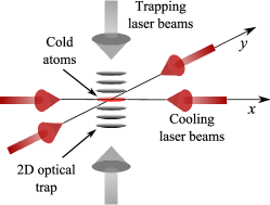
Figure 1: Schematic view of the experimental setup. Atoms are confined in strongly anisotropic, quasi two dimensional, optical dipole traps: they form one or several pancake shaped clouds. Two pairs of orthogonal contra-propagating lasers beams are in quasi-resonance with an atomic transition providing cooling and shadow forces in the x-y plane.

Modeling- We describe one cloud of cold atoms by a two dimensional phase space density $f(\vec{r},\vec{v},t)$, using the shorthands $\vec{r}=(x,y)$, $\vec{v}=(v_{x},v_{y})$. We make the reasonable assumption that cooling can be modeled by a linear friction $-\gamma\vec{v}$, and use a constant velocity diffusion coefficient $D$ to take into account the velocity recoils due to random absorption and fluorescence emission of photons by the atoms. We use the following standard expression for the force $\vec{F}=(F_{x},F_{y})$ for the shadow effect, which relies on a weak absorption limit Dalibard (1988):

$$F_{x}[\rho](x,y) =-C\int\mbox{sgn}(x-x^{\prime})\rho(x^{\prime},y)~{}dx^{\prime}$$ (1a)

$$F_{y}[\rho](x,y) =-C\int\mbox{sgn}(y-y^{\prime})\rho(x,y^{\prime})~{}dy^{\prime}$$ (1b)

where $\rho(x,y)$ is the surface density of atoms, normalized to $1$; $C$ is a constant characterizing the intensity of the force, which can be computed after integration over the transverse direction Chalony et al. (2013):

$$C=\frac{\hbar k\Gamma}{2}\frac{I_{0}}{I_{s}}\frac{N}{(1+4\bar{\delta}^{2})^{2}}\frac{\sigma_{0}}{2\sqrt{\pi}L_{\perp}}.$$ (2)

In this expression, $k$ is the wave number, $\Gamma$ the width of the atomic transition, $\bar{\delta}$ the normalized frequency detuning, $N$ the number of trapped atoms, $\sigma_{0}=6\pi/k^{2}$ the resonant photon absorption cross-section, $L_{\perp}$ the transverse size of the cloud, $I_{0}$ the incident laser intensity and $I_{s}$ the saturation intensity. Note that the shadow force (1) verifies the same Poisson equation as gravity $\vec{\nabla}\cdot\vec{F}\propto-\rho$, but, contrary to gravity, does not derive from a potential, i.e., $\vec{\nabla}\times\vec{F}\neq\vec{0}$.

The optical dipole traps in the x-y plane are well approximated by harmonic traps at frequency $\omega_{0}$ and will be modeled accordingly. Moreover, usual experimental configurations correspond to the overdamped regime, i.e. $\omega_{0}\ll\gamma$. So the velocity distribution quickly relaxes to a Gaussian, and the surface density $\rho(x,y,t)$ evolves according to a non-linear Smoluchowski equation

$$\frac{\partial\rho}{\partial t}=\vec{\nabla}\cdot\left[\frac{\omega_{0}^{2}}{\gamma}\vec{r}\rho+\frac{1}{m\gamma}\vec{F}[\rho]\rho+\frac{k_{B}T}{m\gamma}\vec{\nabla}\rho\right]$$ (3)

where $m$ is the atomic mass, and the temperature is determined by the relation $k_{B}T/m=D/\gamma$.

Rescaling time and space as $\tilde{t}=(\omega_{0}^{2}/\gamma)t$, $(x,y)=(L\tilde{x},L\tilde{y})$ with $L=\sqrt{C/(m\omega_{0}^{2})}$, Eq. (3) becomes (dropping the  $\tilde{}$  for convenience):

$$\frac{\partial\rho}{\partial t}=\vec{\nabla}\cdot\left[\vec{r}\rho+\vec{F}[\rho]\rho+\Theta\vec{\nabla}\rho\right]$$ (4)

This equation is the starting point of our theoretical analysis.

Model analysis- The physics is governed by a single dimensionless parameter

$$\Theta=\frac{k_{B}T}{C}.$$

The above Eq. (4) is similar to the Smoluchowski-Poisson system describing self-gravitating Brownian particles, or the parabolic-elliptic Keller-Segel model used in chemotaxy theoryKellerSegel ; Chavanis1 . However, the force does not derive from a potential. It is well-known that if the temperature is small enough, a solution to the Smoluchowski-Poisson equation blows up in finite time and forms a Dirac peak. This behavior can also be seen as a phase transition in the canonical ensemble. It is natural to ask if the same phenomenology holds for Eq. (4), the non potential generalization of the Smoluchowski-Poisson equation.

To get insight in the behavior of Eq. (4), we compute the time evolution of $S(t)=-\int\rho\ln\rho$. Note that the formation of a Dirac peak corresponds to $S(t)\to-\infty$. Using Eq. (4), $\vec{\nabla}\cdot\vec{F}=-4\rho$ and after integrating by parts, we get

$$\dot{S}(t)=-2-4\int\rho^{2}d^{2}\vec{r}+\Theta\int\frac{|\nabla\rho|^{2}}{\rho}d^{2}\vec{r}~{}.$$ (5)

Writing now $\rho=\sqrt{u}$ and using the functional inequality, valid in 2D Weinstein82 : $\int\!u^{4}\leq a\int\!|\nabla u|^{2}\times\int\!u^{2}$, we have

$$\dot{S}(t)\geq-2+(\Theta-a)\int\!\frac{|\nabla\rho|^{2}}{\rho}d^{2}\vec{r}$$ (6)

where $a$ is a constant, known numerically: $a\simeq 0.171$. If $\Theta>a$, the second term in the right hand side of the inequality is positive and dominates over the first term above a certain spatial density of the cloud. It ensures that $S(t)$ cannot decrease without bound: collapse is excluded. On the other hand, for $\Theta<a$, collapse becomes possible, even though of course this argument cannot prove that it happens. If it happens, we should not expect either $0.171$ to be an accurate estimate of the critical parameter $\Theta_{c}$, but an indication for the behavior of Eq. (4). Indeed, as we describe below, we numerically find indications of a collapse transition at a lower $\Theta$, namely $\Theta\simeq 0.12-0.15$.

Numerical simulations- To simulate Eq.(4), we introduce the following stochastic particles approximation: The position of particle $i$ is denoted by $\vec{r}_{i}=(x_{i},y_{i})$, and the dynamical equations are:

$$\dot{x}_{i} =-x_{i}+F_{i,x}+\sqrt{2\Theta}\eta_{i,x}(t)$$ (7a)

$$\dot{y}_{i} =-y_{i}+F_{i,y}+\sqrt{2\Theta}\eta_{i,y}(t),$$ (7b)

where the $\eta_{i,.}$ are independent gaussian white noises. To define $F_{i,x}$ and $F_{i,y}$ numerically we introduce the spatial scale $\sigma$. The force is then written as

$$F_{i,x} =-C\sum_{j\neq i}\mbox{sgn}(x_{i}-x_{j})\delta_{\sigma}(y_{i}-y_{j})$$ (8a)

$$F_{i,y} =-C\sum_{j\neq i}\mbox{sgn}(y_{i}-y_{j})\delta_{\sigma}(x_{i}-x_{j}),$$ (8b)

where $\delta_{\sigma}(z)=1$ if $|z|<\sigma$ and zero otherwise. In the limit $\sigma\to 0$, Eqs.(8) reduce to the original definition of the force (1). We expect to correctly approximate Eq.(4) when $n\sigma\gg 1$, where $n$ is the number of particles. We integrate the equation of motions using an Euler scheme. The force calculation is sped up using the following procedure: space is discretized with cells of size $\sigma$ and particles are assigned to cells using the linked-list technique (see e.g. knuth_68 ); this is a $\mathcal{O}(n)$ operation which does not involve any approximation. Note that the numerical particles should not be seen as direct representations of the atoms in the trap; however, the spatial distribution of the numerical particles should approximate the 2D spatial distribution of atoms described by (4).

We performed a series of simulations varying initial conditions, $\sigma$ and number of particles $n$, with $\Theta$ in the range $[0.08,0.3]$. In order to keep the strength of the gravitation-like interaction constant when changing the parameters, we keep the quantity $Cn\sigma$ constant. After a time $t\sim 1$, all the simulations reach a stationary state, which we find to be essentially independent of $\sigma$, $n$ (for sufficiently large $n$ and small $\sigma$) and of the initial conditions.

Figure 2: Snapshot of the particles distribution in the stationary state of a system with $\sigma=10^{-2}$, $n=10^{4}$, a time step $\Delta t=10^{-5}$ and (a) $\Theta=0.14$ and (b) $\Theta=0.2$. The laser beams are along the axes of the figure.

In Fig. 2 are shown snapshots of the particles distributions in the stationary state at $\Theta=0.14$ and $\Theta=0.2$. They show a cross-like structure along the diagonals, which is related to the presence of currents as we will discuss latter on. To look for a phase transition toward a collapse phase, we plot the central spatial density as a function of $\Theta$, as shown in Fig. 3. We observe an abrupt increase in the density when $\Theta$ is decreased, for $\Theta_{c}\approx 0.12-0.15$.

\psfrag{X}{$\Theta$}\psfrag{Y}{$\rho(r=0)$}\includegraphics[height=151.76964pt]{density_center.eps}

Figure 3: Density $\rho(r=0)$ in the center of the trap, as a function of the reduced temperature $\Theta$ for $\sigma=10^{-2}$, $n=10^{4}$ and a time step $\Delta t=10^{-5}$. Filled (empty) points correspond to simulations which (do not) have numerically converged with respect to the time step (see text). Inset: Same quantity plotted in linear-linear scale. The two vertical dashed lines indicate the numerically estimated location of the transition $\Theta_{c}\approx 0.12-0.15$.

Furthermore, we note that for all simulations with $\Theta>\Theta_{c}$ the asymptotic state is independent of the time step, suggesting a convergence to a regular stationary state of (4). In contrast, for $\Theta<\Theta_{c}$, we have been unable to reach a stationary state independent of the time step. Hence the numerical results for $\Theta<\Theta_{c}$ should be taken with caution, since no convergence to a regular solution is achieved. Importantly, this lack of convergence suggests as well that the limit system develops a singularity, indicating the presence of the collapsed phase.

A phase transition toward a collapsed phase at a finite temperature parameter $\Theta$ makes our system similar to a 2D self-gravitating gas of Brownian particles, for which the phase transition is predicted at $\Theta_{c}=1/(2\pi)$ (see for example Chavanis2002 ), i.e. at a value slightly larger than the one numerically found here. However, in contrast with a 2D self-gravitating gas, the system is truly out of equilibrium; this can be illustrated by computing the current $\vec{J}$ in the stationary state. Using Eq. (4), we have $\vec{J}=\vec{r}\rho+\vec{F}[\rho]\rho+\Theta\vec{\nabla}\rho$, with $\vec{\nabla}\vec{J}=0$. For interactions deriving from a potential, it is simple to show that, in thermal equilibrium, $\vec{J}=\vec{0}$. In the present case $\vec{J}\neq\vec{0}$, and the inset of Fig. 4 shows their spatial structure. As expected, ingoing currents are along the laser beams where the long-range interaction is maximal. Escaping channels from the trap center are along the diagonals. This current structure explains the cross-like shape found in the particle distribution (see Fig. 2). In the main part of the figure, we see that the current intensity strongly increases as the transition region is approached from above. Like for the central density discussed above, the computed current intensity in the $\Theta<\Theta_{c}$ region should be taken with caution, since the simulations results still depend on the time step.

\psfrag{X}{$\Theta$}\psfrag{Y}{$\langle|\vec{J}|^{2}\rangle$}\includegraphics[height=151.76964pt]{var_flux.eps}

Figure 4: Spatially averaged square intensity of the currents as a function of $\Theta$ for $\sigma=10^{-2}$, $n=10^{4}$ and a time step $\Delta t=10^{-5}$. Filled (empty) points correspond to simulations which (do not) have numerically converged with respect to the time step (see text). The vertical dashed lines indicates the numerically estimated location of the transition region: $\Theta_{c}\approx 0.12-0.15$. Inset: Spatial distribution of current $\vec{J}$ in the stationary state; $\Theta=0.2$. The laser beams are along the axes of the figure.

Possible experimental realization- The experiment could be performed following the scheme depicted in ref. Chalony et al. (2013). The starting point would be a Strontium88 gas, laser cooled in a magneto-optical trap operating on the narrow ${}^{1}\!S_{0}\rightarrow\,^{3}\!P_{1}$ intercombination line at $689\,\textrm{nm}$ Chaneliere et al. (2008). The bare linewidth of the transition is $\Gamma/2\pi=7.5\,\textrm{kHz}$. Ultimately, the gas is transferred into one or several 2D dipole traps made with a far off-detuned high power standing optical wave located along the vertical axis. We expect that the interactions between two parallel 2D traps shall be weak. In the horizontal plane, two pairs of orthogonal contra-propagating laser beams red detuned with respect to the ${}^{1}\!S_{0}\rightarrow\,^{3}\!P_{1}$ narrow transition are turned on (see Fig. 1). This set-up realizes the proposed 2D gravitational-like interaction. In order to avoid any spatial dependency of the quasi-resonant laser beams detuning, the dipole trap wavelength is tuned on the so-called ”magic” wavelength which is $\lambda\sim 900\,\textrm{nm}$ for our particular case Katori et al. (2013). Importantly, the cold cloud has a horizontal pancake shape. This strong shape asymmetry is necessary to reduce the repulsive interaction mediated by the multiple scattering Walker et al. (1990). In this geometry scattered photons are likely to escape the cloud through the transverse direction. Similar requirements were successfully implemented in the one dimensional case Chalony et al. (2013). They also prevent the generalization of this method to three dimensional gravitational systems.

We have to check that the regime where the collapse should take place is within reach of current experimental techniques. For this order of magnitude computation, we use a cold cloud with $N=2\times 10^{6}$ atoms at a temperature of $T=2\,\mu\textrm{K}$. The power of the dipole trap laser beams is $3$W and its waist $300\,\mu\textrm{m}$. The trap depth is $\frac{k_{b}}{2}\times 10\,\mu\textrm{K}$. The transverse cloud size, frozen by the standing wave trapping, is set to $L_{\bot}=5\,\mu\textrm{m}$, whereas the equilibrium longitudinal thermal distribution in the dipole trap and without the quasi resonant laser beams is $L=100\,\mu\textrm{m}$. Modeling the shadow effect by a long-range gravitation-like force requires a weak absorption of the laser beams, i.e. a low optical depth $b<1$; it corresponds here, to a frequency detuning of $|\delta|>5.7\Gamma$. In this range, the minimal dimensionless temperature that should be reachable is around $\Theta\sim 0.07$. This is below the theoretical threshold for collapse, thus the expected phase transition should be observable. One has to make sure however that the weak absorption limit is fulfilled, and thus the model is valid, for a large range of spatial density. Indeed we do not expect strictly speaking a collapse of the atomic cloud since above a certain density necessarily $b>1$. In this latter case, the shadow force becomes short range and the size of the cloud should remain finite. The modeling we have used also requires a low saturation. For this computation, we have assumed a quasi resonant laser intensity $I=14I_{s}$ (where $I_{s}=3\,\mu W/\textrm{cm}^{2}$ is the saturation intensity). It corresponds to a saturation parameter $s=\frac{I/I_{s}}{4(\delta/\Gamma)^{2}+1}<0.1$. Thus the low saturation approximation is fulfilled.

Finally one notices that the experiment can be in principle performed using more standard alkali setup with broad transitions rather than the narrow intercombination line of Strontium. However, it is expected to be technically more challenging with the formers because ”magic” wavelengths are usually more difficult to access Arora et al. (2013) and the dipole trap laser should have a much larger power to maintain the higher temperature gas. Moreover, temperatures close to the Fermi temperature have been reported for laser cooling of the Strontium87 isotope in a 3D trap Mukaiyama et al. (2013). It seems reasonable to believe that the action of laser cooling in combination with the long range attractive force in the 2D trap might bring the gas closer or even below the degeneracy temperature. If such a condition is fulfilled, like for a white dwarf, the Pauli pressure should play a role in the short range stabilization of the gas in the collapse phase. The interplay between the non equilibrium collapse phase and the Pauli pressure remains an open question which should be addressed in a forthcoming publication.

Conclusion- This work paves the way for the experimental observation of a non equilibrium collapse phase transition, driven by a long range interaction force. All the characteristic features on the density and the current, should be observable using the current in-situ or time-of-flight imaging technics. This work also opens the door to outstanding theoretical questions: how could one prove the conjectured collapse? Beyond the entropic computation done here, what could be the tools for such a task? How could one develop a better numerical scheme when the transition is approached?

Acknowledgments: We thank Y. Brenier, M. Chalony, D. Chiron, T. Goudon, M. Hauray, P.E. Jabin and A. Olivetti for useful discussions. This work was partly supported by the ANR 09-JCJC-009401 INTERLOP project and the CNPq (National Council for Scientific Development, Brazil).

References

- (1) G. Ódor, Rev. Mod. Phys., 76, 663 (2004).
- (2) A. Coniglio, Phys. Rev. Lett., 46, 250 (1981).
- (3) H. Hinrichsen, Ad. in Phys., 49, 815 (2000).
- (4) M. Berhanu et a.l., Europhys. lett. 77 59001 (2007).
- (5) K. R. S tterlin et al. 2010 Plasma Phys. Control. Fusion 52, 124042 (2010).
- (6) A. L. Barabási and H. Stanley, Fractal concepts in surface growth (Cambridge University Press, U.K., 1995).
- (7) P. Krogstrup et a.l., J. Phys. D: Appl. Phys, 6 313001 (2013).
- (8) D. E. Wolf, M. Schreckenberg, and A. Bachem, Traffic and granular flow (World Scientific, Singapore, 1996).
- (9) M. Henkel, H. Hinrichsen and S. Lübeck, Non-Equilibrium Phase Transitions (Springer, 2009).
- Antonov (1961) V. Antonov, Soviet Astr.-AJ 4, 859 (1961).
- Lynden-Bell and Wood (1968) D. Lynden-Bell and R. Wood, Monthly Notices of the Royal Astronomical Society 138, 495 (1968).
- (12) M. Kiessling, J. Stat. Phys. 55, 203 (1989).
- Thirring (1970) W. Thirring, Zeitschrift für Physik A 235, 339 (1970).
- (14) P.H. Chavanis, C. Rosier and C. Sire Phys. Rev. E 66, 036105 (2002).
- (15) C. Sire and P.H. Chavanis, Phys. Rev. E 66, 046133 (2002).
- Dalibard (1988) J. Dalibard, Opt. Comm. 68, 203 (1988).
- Chalony et al. (2013) M. Chalony, J. Barré, B. Marcos, A. Olivetti, and D. Wilkowski, Phys. Rev. A 87, 013401 (2013).
- (18) P.H. Chavanis, Astron. Astrophys. 381, 340 (2002).
- (19) E.F. Keller and L.A. Segel J. Theor. Biol. 30, 225 (1971).
- (20) M. I. Weinstein, Nonlinear Schrödinger equations and sharp interpolation estimates, Comm. Math. Phys. 87, 567 (1982/83).
- (21) Knuth, D. E., em The Art of Computer Programming, Addison-Wesley, Reading, MA, 1968.
- Chaneliere et al. (2008) T. Chaneliere, L. He, R. Kaiser, and D. Wilkowski, Eur. Phys. J. D 46, 507 (2008).
- Katori et al. (2013) H. Katori, T. Ido, and M. Kuwata-Gonokami, J. Phys. Soc. Jpn. 68, 2479 (1999).
- Walker et al. (1990) T. Walker, D. Sesko, and C. Wieman, Phys. Rev. Lett. 64, 408 (1990).
- Arora et al. (2013) B. Arora, M. S. Safronova, and C. W. Clark, Phys. Rev. A 76, 052509 (2007).
- Mukaiyama et al. (2013) T. Mukaiyama, H. Katori, T. Ido, Y. Li, and M. Kuwata-Gonokami, Phys. Rev. Lett. 90, 113002 (2003).