Likelihood analysis for a class of beta mixed models

Abstract

Beta regression is a suitable choice for modelling continuous response variables taking values on the unity interval. Data structures such as hierarchical, repeated measures and longitudinal typically induce extra variability and/or dependence and can be accounted for by the inclusion of random effects. Statistical inference typically requires numerical methods, possibly combined with sampling algorithms. This class of Beta mixed models is adopted for the analysis of two real problems with grouped data structures. We focus on likelihood inference and describe the implemented algorithms. The first is a study on the life quality index of industry workers with data collected according to an hierarchical sampling scheme. The second is a study assessing the impact of hydroelectric power plants upon measures of water quality indexes up, downstream and at the reservoirs of the dammed rivers, with a nested and longitudinal data structure. Results from different algorithms are reporter for comparison including from data-cloning, an alternative to numerical approximations which also allows assessing identifiability. Confidence intervals based on profiled likelihoods are compared to those obtained by asymptotic quadratic approximations, showing relevant differences for parameters related to the random effects. In both cases the scientific hypothesis of interest were investigated by comparing alternative models, leading to relevant interpretations of the results within each context.

keywords: hierarchical models, likelihood inference, Laplace approximation, data-cloning, life quality, water quality

1 Introduction

Response variables in the form of proportions, rates and indexes are common to different areas such as economics, social and environmental sciences. They are typically measured in the interval $(0,1)$. This makes the usual linear (Gaussian) regression model inappropriate since it does not ensures predicted values confined to the unity domain nor is able capture asymmetries.

Several alternative models are considered in the literature. Kieschnick and McCullough (2003) provides an overview and, based on the results of several case studies, advocates the adoption of beta regression models. This is regarded as a flexible class given the diversity of possible shapes for the distribution function.

Regression models for independent and identically beta distributed variables are described by Paolino (2001), Cepeda (2001), Kieschnick and McCullough (2003) and Ferrari and Cribari-Neto (2004). The modelling inherits from the principles of generalised linear models (Nelder and Wedderburn, 1972), relating the expected value of the response variable to covariates through a suitable link function. Cepeda (2001), Cepeda and Gamerman (2005) and Simas et al. (2010) extend the models regressing both, mean and dispersion parameters on potential covariates. The latter also considers non-linear forms for the predictor. Smithson and Verkuilen (2006) explores the beta regression with an application to IQ data, arguing it provides a prudent and meaningful choice compared to alternative approaches. The beta distribution is able to capture strongly skewed data, bounded above and below. It accommodates heterocedasticy, and allows for testing hypothesis on location and dispersion separately whilst being parsimonious with only two parameters, likewise the Gaussian linear model.

Methods for likelihood based inference and model assessment are adopted by Espinheira et al. (2008b), Espinheira et al. (2008a) and Rocha and Simas (2011). Bias correction for likelihood estimators are developed by Ospina et al. (2006), Ospina et al. (2011) and Simas et al. (2010). Branscum et al. (2007) analyses virus genetic distances under the Bayesian paradigma. The beta regression is implemented by the betareg package (Cribari-Neto and Zeileis, 2010) for the R environment for statistical computing (R Development Core Team, 2012). Extended functionality is added for bias correction, recursive partitioning and latent finite mixture (Grün et al., 2012). Mixed and mixture models are discussed by Verkuilen and Smithson (2012). Time series dependence structure is considered by McKenzie (1985), Grunwald et al. (1993) and Rocha and Simas (2011). More recently da Silva et al. (2011) adopts a Bayesian beta dynamic model for modelling and prediction of time series with an application to the Brazilian unemployment rates.

Dependence structures may arise in other contexts such hierarchical model structures, longitudinal and split-plot designs or any other form of grouping in the sampling mechanism. Correlation between observations within the same group can be induced by inclusion of random effects in the model. The total variability is therefore decomposed in within and between groups effects. As for usual generalised linear mixed models, the beta mixed models allow for dependent and overdispersed data by inclusion of random effects, typically assumed to be Gaussian distributed. Generalised linear mixed models and ordinary beta regression models are widely discussed in the literature, but not beta mixed models, which have recently being considered under the Bayesian perspective by Figueroa-Zúñiga et al. (2013).

Our main goal is to model bounded responses by beta mixed models, adopting likelihood based methods of inference and with discussions in the context of the analysis of two real data sets. The first is a study on the life quality index of industry workers with data grouped on a hierarchical structure. The second is a comparison of water quality indexes measured upstream and downstream hydroelectric power plant reservoirs, with data grouped on a longitudinal structure. The beta mixed model is regarded as a natural choice for both examples.

Inference require numerical methods since the likelihood function involves an integral which cannot be solved analytically. We consider Gaussian quadrature, quasi Monte Carlo and Laplace approximations when integrating the random effects when evaluating the likelihood function. We also consider a Markov chain Monte Carlo (MCMC) based algorithm proposed by Lele et al. (2007) for likelihood inference for generalized linear mixed models which also allows investigating identifiability. Laplace approximation is less demanding on computing time and suitable for model selection, whereas the latter is suitable for further assessment of the best fitted models. Results are compared with the ones obtained with the computationally less demanding linear and non-linear mixed models.

The beta regression model including random effects and the adopted methods for likelihood inference are described in Section 2. The two motivating examples are presented in Section 3, illustrating the flexibility of the model in accounting for relevant features of the data structures which would be neglected under a standard beta regression assuming independent observations. The two examples have different justifications and structures for the random effects. The first specifies two, possibly correlated, random effects whereas the second has a nested random effects structure as a parsimonious alternative to a fixed effects model. We compare results obtained with different models and algorithms and close with concluding remarks on Section 5.

2 Beta mixed models

Let $Y\sim B(\mu,\phi)$ denote a beta distributed random variable with density function

$$f(y|\mu,\phi)=\frac{\Gamma(\phi)}{\Gamma(\mu\phi)\Gamma((1-\mu)\phi)}y^{\mu\phi-1}(1-y)^{(1-\mu)\phi-1},\quad 0<y<1,$$ (1)

parametrized in terms of mean and dispersion parameters (Jørgensen, 1997a, b), where $\Gamma(.)$ is the Gamma function, $0<\mu<1$, $\phi>0$ is a dispersion parameter, $E(Y)=\mu$ and $V(Y)=\frac{\mu(1-\mu)}{(1+\phi)}$. For response variables $Y_{i}\sim B(\mu_{i},\phi)$, the beta regression model (Ferrari and Cribari-Neto, 2004) specifies a linear predictor $\eta_{i}=g(\mu_{i})=\mathbf{x}_{i}^{T}\boldsymbol{\beta}$, with $\boldsymbol{\beta}=(\beta_{1},\ldots,\beta_{k})^{T}$ a vector of the $k$ unknown regression coefficients and $\mathbf{x}_{i}=(x_{i1},\ldots,x_{ik})^{T}$ a vector of $k$ covariates. For the link function $g(\cdot):(0,1)\to\Re$ we adopt the logit $g(\mu)=\log({\mu/(1-\mu)})$. Other usual choices are the probit, complementary log-log and cauchit (Cribari-Neto and Zeileis, 2010).

This model does not contemplate possible dependencies such those as induced by multiple measurements on the same observational unit, over time or space. Inclusion of latent random effects on grouped data structure is a parsimonious strategy compared to adding parameters to the fixed part of the model whilst still accounting for nuisance effects. The random effect model can be specified as follows. Denote $y_{ij}$ an observation $j=1,\ldots,n_{i}$ within group $i=1,\ldots,q$ and $\mathbf{y}_{i}$ denote a $n_{i}$-dimensional vector of measurements from the $i^{th}$ group. Let $\mathbf{b}_{i}$ be a $q$-dimensional vector of random effects and assume the responses $Y_{ij}$ conditionally independent with density given by (1) and $g(\mu_{ij})=\mathbf{x}_{ij}^{T}\boldsymbol{\beta}+\mathbf{z}_{ij}^{T}\mathbf{b}_{i}$, where $\mathbf{x}_{ij}$ and $\mathbf{z}_{ij}$ are vector of known covariates with dimensions $p$ and $q$, respectively, $\boldsymbol{\beta}$ is a $p$-dimensional vector of unknown regression parameters and $\phi$ is the dispersion parameter. The model specification is completed assuming Gaussian random effects $[\mathbf{b}_{i}|\Sigma]\sim N(\mathbf{0},\Sigma)$.

2.1 Parameter estimation

The model parameters can be estimated by maximising the marginal likelihood obtained by integrating the joint distribution $[\mathbf{Y},\mathbf{b}]$ over the random effects. The contribution to the likelihood for the $i^{th}$ group is

$$f_{i}(\mathbf{y}_{i}|\boldsymbol{\beta},\Sigma,\phi)=\int\prod_{j=1}^{n_{i}}f_{ij}(y_{ij}|\mathbf{b}_{i},\boldsymbol{\beta},\phi)f(\mathbf{b}_{i}|\Sigma)d\mathbf{b}_{i}.$$

Assuming independence among the $q$ groups, the full likelihood is given by

$$L(\boldsymbol{\beta},\Sigma,\phi)=\prod_{i=1}^{q}f_{i}(\mathbf{y}_{i}|\boldsymbol{\beta},\Sigma,\phi).$$ (2)

Evaluation of (2) requires solving the integral $q$ times. For the simpler model with a single random effect the integrals are unidimensional. More generally, the dimension equals the number of random effects in the model which imposes practical limits to numerical methods and approximations required to evaluate the likelihood. The integrals in our examples have up to five dimensions and are solved by Laplace approximation (Tierney and Kadane, 1986) for the results reported here. The marginal likelihood is maximised by the algorithm BFGS (Byrd et al., 1995) as implemented in R. During our analysis we tried different methods to integrate out the random effects: Laplace approximation, Gaussian Quadrature and quasi Monte Carlo. No differences we detected up to the second decimal place in the maximised likelihoods.

We have also considered the sampling based data cloning algorithm (Lele et al., 2007), proposed in the context of maximum likelihood estimation for generalised linear mixed models. Data cloning provides tools to assess identifiability (Lele et al., 2010) which we believe is worth exploring for the beta mixed model.

The data-cloning algorithm is based on replicating (cloning) $K-times$ the observations $\mathbf{y}_{i}$ from each group generating $N\times K$ cloned data denoted by $\mathbf{y}_{i}^{K}$. The corresponding likelihood $L^{K}(\boldsymbol{\beta},\Sigma,\phi)$ has the same maximum as (2) and Fisher information matrix equals $K$ times the original information matrix. The method relies on the Bayesian approach to construct a Monte Carlo Markov chain - MCMC (Robert and Casella, 2005) algorithm and using the fact the effect of prior vanishes as the number of clones is increased. The model is therefore completed by the specification of priors $\pi(\boldsymbol{\beta})$, $\pi(\Sigma)$ and $\pi(\phi)$, which combined with the cloned likelihood, lead to a posterior of the form

$$\pi_{K}(\boldsymbol{\beta},\Sigma,\phi|y_{ij})=\frac{[\int f_{i}(\mathbf{y}_{i}|\boldsymbol{\beta},\Sigma,\phi)f(\mathbf{b}_{i}|\Sigma)d\mathbf{b}_{i}]^{K}\pi(\boldsymbol{\beta})\pi(\Sigma)\pi(\phi)}{C(K;y_{ij})}$$

with the normalising constant

$$C(K;y_{ij})=\int[\int f_{i}(\mathbf{y}_{i}|\boldsymbol{\beta},\Sigma,\phi)f(\mathbf{b}_{i}|\Sigma)d\mathbf{b}_{i}]^{K}\pi(\boldsymbol{\beta})\pi(\Sigma)\pi(\phi)d\boldsymbol{\beta}d\Sigma d\phi.$$

MCMC algorithms provide a sample from the posterior. By increasing the number $K$ of clones, the posterior mean should converge to the maximum likelihood estimator and $K$ times the posterior variance should correspond to the asymptotic variance of the MLE (Lele et al., 2010). Priors are used to run the algorithm without affecting inference as the likelihood can be arbitrarilly weighted by increasing the number of clones to the point that the effect of priors are negligible.

Despite the flexibility of the inferential mechanism, usual concerns regarding the specification of hierarchical models apply. Realistic and suitable models for the problem and available data can be complex and need to be balanced against identifiability, not often checked nor trivial (Lele, 2010).

Data cloning provides a straightforward identifiability check which can be used for hierarchical models in general. Lele et al. (2010) shows that under non-identifiability, the posterior converges to the prior truncated on the non-identifiability space when the number of clones is increased. As a consequence, the largest eigenvector of the parameter’s covariance matrix does not converges to zero. More specifically, if identifiable, the posterior variance of a parameter of interest should converge to zero when increasing the number of clones.

2.2 Prediction of random effects

Prediction of random effects are typically required as for the examples considered here. Under the Bayesian paradigm the predictions can be directly obtained from the posterior distribution of the random effects given by

$$f_{i}(\mathbf{b}_{i}|\mathbf{y}_{i},\boldsymbol{\beta},\Sigma,\phi)=\frac{f_{i}(\mathbf{y}_{i}|\mathbf{b}_{i},\boldsymbol{\beta},\phi)f(\mathbf{b}_{i}|\Sigma)}{\int f_{i}(\mathbf{y}_{i}|\mathbf{b}_{i},\boldsymbol{\beta},\phi)f(\mathbf{b}_{i}|\Sigma)d\mathbf{b}_{i}},$$

which does not have a closed expression for the beta model. The posterior mode maximizes $f_{i}(\mathbf{y}_{i}|\mathbf{b}_{i},\boldsymbol{\beta},\phi)f(\mathbf{b}_{i}|\Sigma)$ providing a point predictor for $\hat{\mathbf{b}}_{i}$ and empirical Bayes predictions can be obtained by replacing the unknown parameters by their maximum likelihood estimates.

3 Examples

3.1 Income and life quality of Brazilian industry workers

The Brazilian industry sector worker’s life quality index (IQVT, acronym in Portuguese) combines 25 indicators from eight thematic areas: housing, health, education, integral health and workplace safety, skill development, work attributed value, corporate social responsibility, participation and performance stimulus. The index is constructed following the same premisses of the united nations human development index. Values are expressed in the unity interval and the closer to one, the higher the industry’s worker life quality.

A pool was conducted by the Industry Social Service in order to assess worker’s life quality in the Brazilian industries. The survey included $365$ companies from nine out of the $27$ Brazilian federative units. IQVT was computed for each company from questionnaires applied to workers according to a sampling design. Companies provided additional information on budget for social benefits and other quality of life related initiatives.

A suitable model is aimed to assess the effects on IQVT of two company related covariates, average namely income and size. The first is simply the total of salaries divided by the number of workers expressing the capacity to fulfil individual basic needs such as food, health, housing and education. The second reflects the industry’s quality of life management capability. There is a particular interest in learning whether larger companies with 500 or so workers, typically multinational, working under regimes of worldwide competition, provide better life standards in comparison with medium (100 to 499 workers) and small (20 to 99 workers) sized industries. The federative unit where the company is located is expected to be influential due to varying local legislations, taxing and further economic and political conditions. Plots on Figure 1 suggests IQVT is associated with income, size and location. The income is expressed in logarithmic scale centred around their average.

Figure 1: IQVT related to (centred log) average income, company size and federative unit.

The beta random effects model for IQVT is

$$Y_{ij}|\mathbf{b}_{i} \sim B(\mu_{ij},\phi)$$

$$g(\mu_{ij}) =(\beta_{0}+b_{i1})+\beta_{1}Medium_{ij}+\beta_{2}Small_{ij}+(\beta_{3}+b_{i2})Income_{ij}$$

$$\mathbf{b}_{i} \sim NMV(\mathbf{0},\Sigma)\mbox{ with }\Sigma=\left[\begin{array}[]{rr}1/\tau_{1}^{2}&\rho\\ \rho&1/\tau_{2}^{2}\\ \end{array}\right],$$

parametrized such that $\beta_{0}$ is associated with large sized companies and $\beta_{1}$ and $\beta_{2}$ are differences for the medium and small sized companies, respectively. A random intercept $b_{i1}$ and slope $b_{i2}$ associated with income account for the effect of the federative units. Model parameters to be estimated consist of the regression coefficients $(\beta_{0},\beta_{1},\beta_{2},\beta_{3})$, the random effects covariance parameters $(\tau_{1}^{2},\tau_{2}^{2},\rho)$ and the precision parameter $\phi$.

A sequence of sub-models are defined for testing relevant effects. Model 1 is the null model with simply the intercept. Model 2 includes the covariate size and Model 3 the income. Model 4 adds random intercepts and Model 5 adds a random slope to income. For comparison, we also fit the corresponding linear mixed Gaussian (LMM) and non-linear logistic models (NLMM), widely used in practice.

Parameter estimates for the beta models using Laplace approximation for the random effects are given in the top part of Table 1 and maximised log-likelihoods for the five model structures are given in Table 1 along with the ones for the linear and non-linear models.

Table 1: Parameter estimates for the beta models (top) and maximised likelihood for the alternative models (bottom) - IQVT.

Parameter	Model 1	Model 2	Model 3	Model 4	Model 5
$\beta_{0}$	0.35	0.45	0.43	0.40	0.40
$\beta_{1}$		-0.11	-0.09	-0.07	-0.07
$\beta_{2}$		-0.16	-0.14	-0.13	-0.13
$\beta_{3}$			0.42	0.47	0.47
$\phi$	53.97	56.80	72.86	94.19	94.19
$\tau_{1}^{2}$				62.36	62.35
$\tau_{2}^{2}$					51480.17
$\rho$					0.85
Model	Maximised likelihood
Beta	472.20	481.51	526.94	561.79	561.80
LMM	470.42	479.96	523.85	558.89	558.90
NLMM	470.42	479.96	523.77	558.96	558.96

Comparison of models 1-3 confirms the relevance of the covariates with estimates of the precision parameter $\phi$ increasing from $53.97$ on Model 1 to $72.85$ on Model 3. The random intercept added in Model 4 clearly further improves the fit expressing the variability of the IQVT among the federative units with an increase of $34.85$ in the log-likelihood. Addition of the random slope did not prove relevant. Model 4 including the two covariates and just the random intercept is therefore the model of choice.

The beta mixed model is not commonly adopted in the literature and this motivates us to consider the data cloning as a distinct approach for likelihood computations which also allows for assessing the model identifiability. The results are reassuring with similar estimates and standard errors obtained by maximization of the numerically integrated marginal likelihood and data cloning as shown in Table 2.

Table 2: Parameter estimates and standard errors for Model 4 by marginal likelihood and data-cloning - IQVT.

Parameter	Marginal likelihood		Data-clone
	Estimate	Std. error	Estimate	Std. error
$\beta_{0}$	0.40	0.05	0.40	0.05
$\beta_{1}$	-0.07	0.03	-0.07	0.03
$\beta_{2}$	-0.13	0.03	-0.13	0.03
$\beta_{3}$	0.47	0.04	0.47	0.04
$\phi$	94.19	7.03	94.17	6.98
$\tau_{1}^{2}$	62.36	32.00	62.03	32.08

Interval estimates obtained by both, the asymptotic quadratic approximation with standard errors returned by data cloning and by profiling the marginal likelihoods are presented in Table 3. The latter can be asymmetric and with coverages closer to nominal values. Intervals are similar for all the parameters except for $\tau_{1}^{2}$ with an artefactual negative lower bound for the quadratic approximation.

Table 3: Asymptotic and profile likelihood based confidence intervals, Model 4 - IQVT.

Parameter	Asymptotic		Profile
	2.5%	97.5%	2.5%	97.5%
$\beta_{0}$	0.30	0.50	0.29	0.50
$\beta_{1}$	-0.13	-0.02	-0.13	-0.02
$\beta_{2}$	-0.19	-0.07	-0.19	-0.07
$\beta_{3}$	0.39	0.55	0.39	0.55
$\phi$	80.49	107.84	81.09	108.65
$\tau_{1}^{2}$	-0.85	124.91	19.74	156.48

Identifiability can be assessed by the data cloning method as described in Section 2. We use the package $dclone$ (Sólymos, 2010), with the JAGS (Plummer, 2003) MCMC engine with $1$, $5$, $10$, $20$, $30$, $40$ and $50$ clones. For each number of clones we use $3$ independent chains of size $6500$, and burn-in of $1500$. Results are summarised in Figure 2 with chains increasingly concentrated around the maximum likelihood estimate with increasing number of clones.

Figure 2: Sampled parameter values for different number of clones, Model 4 - IQVT.

Figure 2 also allows comparison between results for usual Bayesian inference ($K=1$) with for the $K$ fold cloned data. The adopted flat normal prior (zero mean and precision $0.001$) for the regression parameters was not influential whereas the Gamma$(1,0.001)$ prior for $\phi$ and $\tau_{1}^{2}$ showed different results for $K=1$ and $K=50$.

Under identifiability, the posterior variance should converge to zero for increasing number of clones $K$ with variance decreasing at rates $1/K$. Such trend is detected as shown in Figure 3 which uses logarithmic scales to ease the visualisation. Variances decrease satisfactorily at nearly expected rates with a slight but not relevant difference for the $\tau_{1}^{2}$ parameter supporting the conclusion that Model 4 is identifiable for the current data.

Figure 3: Identificability diagnostics with data-cloning for the beta model with random intercept - IQVT.

Fitted coefficients support the initial conjectures that the size has a relevant effect on the IQVT with expected decrease of $3.01\%$ and $5.70\%$ changing from large to medium and small sizes, respectively. These predictions are obtained setting the other factors to baseline and/or zero values. Increasing income clearly positively affects the IQVT, confirming and quantifying the expected behaviour. The fitted random intercepts confirm the existence of a substantial variation in the quality of life among the federative units. Table 4 summarises IQVT predicted for different federative units and company sizes and computed for lower (R$\$500.00$) and higher (R$\$2,500.00$) levels of income.

Table 4: Predicted indexes and percent differences (within parenthesis) to the global average for Model 4 - IQVT.

Fed.	R$ 500,00			R$ 2.500,00
Unity	Large	Medium	Small	Large	Medium	Small
AM	52.91(1.52)	51.11(1.58)	49.60(1.63)	70.55(0.95)	69.02(1.00)	67.72(1.04)
CE	54.48(4.52)	52.68(4.70)	51.17(4.85)	71.84(2.80)	70.35(2.95)	69.08(3.07)
DF	46.5(-10.77)	44.71(-11.13)	43.23(-11.43)	64.95(-7.06)	63.29(-7.39)	61.88(-7.68)
MT	50.82(-2.49)	49.01(-2.58)	47.51(-2.65)	68.78(-1.58)	67.21(-1.66)	65.87(-1.73)
MS	54.22(4.04)	52.42(4.20)	50.92(4.33)	71.63(2.51)	70.14(2.64)	68.86(2.75)
PB	56.91(9.20)	55.13(9.58)	53.64(9.90)	73.79(5.60)	72.37(5.90)	71.15(6.16)
PR	53.83(3.29)	52.03(3.42)	50.52(3.52)	71.31(2.04)	69.81(2.15)	68.52(2.24)
RO	49.17(-5.66)	47.36(-5.86)	45.86(-6.03)	67.34(-3.64)	65.73(-3.82)	64.36(-3.97)
RR	50.11(-3.85)	48.31(-3.99)	46.80(-4.1)	68.17(-2.45)	66.58(-2.58)	65.22(-2.68)

Table 4 shows positive effects for Mato Grosso do Sul (MS), Paraná (PR), Amazonas (AM), Ceará (CE) and Paraíba (PB) with the latter being the best case where IQVT was $9.9\%$ above the global average for small size business with average income of $R\$500.00$. Negative effects were estimated for Mato Grosso (MT), Roraima (RR), Rondônia (RO) and Distrito Federal (DF) being the worse case with IQVT $11.43\%$ below the global average.

The differences for incomes around R$\$500.00$ become smaller for incomes around R$\$2,500.00$, indicating a decreasing influence of company size and federative unity for increasing incomes. The more pronounced effect for low incomes are compatible with Brazilian conditions. There are several governmental supporting policies which effectively improve quality of life for low income workers such as the social assistance unified system, the young agents programme, social and food security, food support, popular restaurants, community catering, family health, maintenance allowance, development educational fund among other Brazilian governmental social programs. Additionally companies internal supporting incentives for low income workers such as catering, transportation, basic shopping supply, among others, make the workplace relevant for the worker quality of life. On the other hand, the higher the income, the lesser the dependence on such benefits and income becomes the main, if not the single, maintainer of life quality and therefore less influenced by conditions such as those reflected by industry size and federative unit. Interpretations based on the fitted model are therefore compatible with the subjective information about the working circumstances in the country. The observed data and fitted values for the random intercept model for each business size is shown on Figure 4.

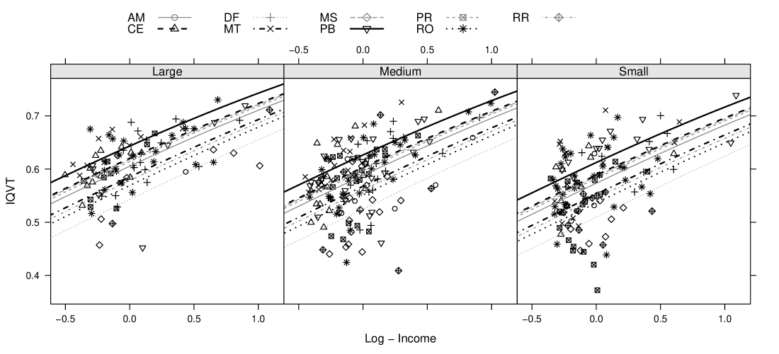
Figure 4: Observed and fitted values for the random intercept model for each business size.

Figure 4 shows IQVT values concentrated between $0.35$ and $0.80$ and within this range the relation with the log-income is nearly linear with a satisfactory adherence to the data. Apparent outliers did not show influence on the overall model fit.

3.2 Water quality on power plant reservoirs

The energy company COPEL operates 16 hydroelectric power plants in Paraná State, Brazil, generating over 4.500 MW. The reservoir lakes are also used for leisure activities, navigation and water supply. Effective functioning of the power plants depends on the quality of the water, which affects the growth of organisms and aquatic flora. Assessing possible impacts of the reservoirs on water quality is relevant for the water supply and environmental hazards. In compliance with operating licenses, the concessionaire company regularly monitors the water quality upstream, downstream and at the reservoirs of the dammed rivers.

Monitoring is based on the comparison of nine water quality indicators against reference values given by standards for water supply. The water quality indicators are: dissolved oxygen, temperature, faecal coliform, water pH, biochemical oxygen demand (DBO), total nitrogen, total phosphorus, turbidity and total solids. The indicators are also combined to produce a single value of a water quality index (IQA, acronym in Portuguese) based upon a study conducted in the 70’s by the US National Sanitation Foundation and adapted by the Brazilian company CETESB.

Monitoring aims to detect changes in the water quality, possibly attributable to the presence of the dams. Water quality measurements taken at locations considered directly affected and unaffected by the reservoir are compared. More specifically, measurements taken upstream the main river are considered unimpacted reference values whereas measurements taken at the reservoir and downstream are considered potentially affected by the water contention and passage throughout the power plant.

Water quality indicators are measured quarterly on the 16 operating hydroelectric power plants and we consider the data collected during 2004. The main interest is the covariate Local, with levels upstream, reservoir and downstream controlled for effects of the power plant and the quarter of data collection. This amounts to 190 data with 12 measurements (4 quarters $\times$ 3 locations) for each of the 16 power plants with only two missing data.

Figure 5: Summaries for the IQA data.

The left asymmetry in Figure 5-A is typical for this kind of data. IQA varies between power plants as seen in 5-B. Figure 5-C suggests an increase from upstream to the reservoir and a decrease from reservoir to downstream. Figure (5-D) shows lower values for the first and forth quarters, the warmer periods, a pattern expected to be repeated over the years.

This brief exploratory analysis suggests that in order to investigate the effect of the position relative to the dam (Local), the effects of quarter and power plant should be accounted for, possibility with distinct quarter effects for different plants. Main effects and interactions would amount for 80 degrees of freedom under a fixed effects model. Instead, we regard the power plants as a sample from a population of environments and add a corresponding random effect term in the model. This is a convenient assumption for our intended method of analysis and proved sound for this particular application.

IQA on the the $i^{th}$ relative location, $j^{th}$ power plant e $t^{th}$ quarter is modelled by

$$Y_{ijt}|b_{j},b_{jt} \sim B(\mu_{ijt},\phi)$$

$$g(\mu_{ijt}) =\beta_{0}+\beta_{1i}+\beta_{2t}+b_{j}+b_{jt}$$

$$b_{j} \sim N(0,\tau_{U}^{2})\;\;;\;\;b_{jt}\sim N(0,\tau_{UT}^{2}),$$

Under the adopted parametrization, $\beta_{1i}$, $i=2,3$ quantifies the changes from upstream to reservoir and downstream, respectively. Likewise $\beta_{2t}$, $t=2,3,4$ are differences between the first quarter and the others. The random intercept $b_{j}$ captures the deviations of each power plant to the overall mean and $b_{jt}$ are the random effects of each quarter within each power plant.

Hypotheses of interest are tested comparing submodels defined by adding terms $\beta_{1i}$, $\beta_{2j}$, $b_{j}$ and $b_{jt}$ sequentially up to the full model. Parameter estimates are presented in Table 5. Numerical estimates are obtained by the BFGS algorithm for maximizing the marginal likelihood with Laplace approximation for the numerical integration of the random effects. The difference of only $1.1091$ between Model 5 and 6 indicates unnecessary the inclusion of $b_{jt}$.

Table 5: Parameter estimates for the beta models (top) and maximised likelihood for the alternative models (bottom) - IQA.

Parameter	Model 1	Model 2	Model 3	Model 4	Model 5	Model 6
$\beta_{0}$	1.40	1.27	1.14	1.14	1.15	1.15
$\beta_{12}$		0.23	0.23	0.24	0.24	0.24
$\beta_{13}$		0.15	0.15	0.16	0.15	0.16
$\beta_{22}$			0.21	0.22	0.22	0.22
$\beta_{23}$			0.29	0.31	0.32	0.32
$\beta_{24}$			0.05	0.05	0.06	0.06
$\phi$	23.36	24.25	25.78	30.47	42.19	42.20
$\tau_{U}^{2}$				28.97		43.54
$\tau_{UT}^{2}$					11.19	15.04
Model	Maximised likelihood
Beta	215.38	218.90	224.62	231.04	237.08	238.19
LMM	198.23	202.12	208.68	213.68	220.39	225.01
NLMM	198.23	202.12	208.72	214.88	223.12	223.91

The likelihood evaluation for the largest model requires numerical approximation of a five dimensional integral, for each reservoir. Dimensionality of the integrals greatly increases the computational burden for the algorithms based on Gauss-Hermite, Monte-Carlo integration or Laplace approximation. The alternative data-cloning algorithm does not demand integral approximation nor numerical maximization and the computational burden is determined by the sampling strategy and fits for increasing number of clones. Table 6 presents the parameter estimates for Model 5 obtained by both ways, integration by Laplace approximation and data-cloning. The regression coefficients are similar however with differences on the standard errors. Overall, smaller values were obtained with the numerically integrated marginal likelihood which demanded more accurately recomputing of the numerical Hessian for the fitted model.

Table 6: Parameter estimates and standard errors for Model 5 by marginal likelihood and data-cloning - IQA.

Parameter	Marginal likelihood		Data-clone
	Estimate	Std. error	Estimate	Std. error
$\beta_{0}$	1.15	0.09	1.15	0.10
$\beta_{12}$	0.24	0.05	0.24	0.07
$\beta_{13}$	0.15	0.01	0.15	0.07
$\beta_{22}$	0.22	0.01	0.22	0.13
$\beta_{23}$	0.32	0.03	0.31	0.13
$\beta_{24}$	0.06	0.01	0.06	0.13
$\phi$	42.19	4.14	42.30	5.32
$\tau_{UT}^{2}$	11.19	3.31	10.99	3.12

Quadratic approximation of the likelihood does not hold and symmetric confidence intervals based on the standard deviations are clearly inappropriate for parameters $\phi$ e $\tau_{UT}$ for which we compute intervals based on profile likelihoods. Right hand panels of Figure 6 show the profile likelihoods for the precision parameters reparametrised on the logarithmic scale for computational convenience. Left hand and middle panels are data-cloning identifiability diagnostic plots. The profile likelihood for $\log(\tau_{UT})$ is asymmetric with this parameter being more sensitive than $\phi$ to the choice of prior, as indicated by the comparison of boxplot for original ($K=1$) and cloned data. The scaled variance plots for $\log(\tau_{UT})$ shows a slightly faster than expected decay in variance for the corresponding number of clones, however the larger eigenvalue for the covariance matrix were found to be always smaller than 1.1, an indicator of identifiability.

Figure 6: Identifiability diagnostic plots and profile likelihoods for precision parameters under Model 5 - IQA.

Empirical Bayes predictions of the random effects are connected by lines in Figure 7. Setting random effects to zero, the fitted model predicts that the IQA increases $5.39\%$ from upstream to the reservoir and $3.55\%$ from up to downstream. The analysis confirms lower IQA values for the warmer temperatures first and forth quarters compared with the milder temperatures second and third quarters. This is expected to be a cyclic behaviour over the years. Significance of random effects implies that the differences vary between power plants and quarters. In summary, the overall pattern is that the IQA substantially improves from upstream to the reservoir however shifting back closer to the original values downstream, however with substantial variation of the differences between the power plants.

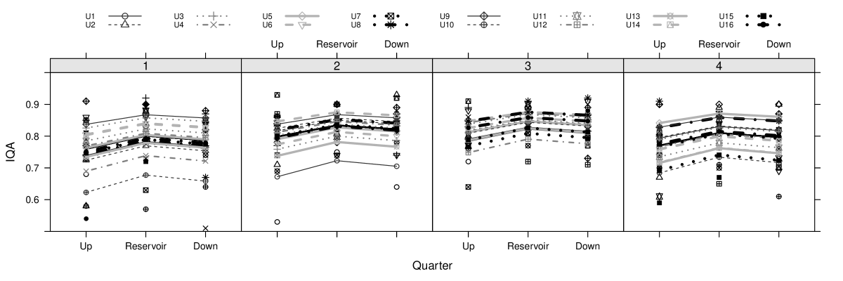
Figure 7: Predicted values under Model 5 connected by lines - IQA.

The adopted model and the algorithms implementing inferential methods proved satisfactory. Some extreme measurements taken upstream in the first and second quarters are smoothed out. Differences between quarters suggest a temporal structure which could be included if modelling observations from consecutive years. A wider range of IQA values for the first and forth quarter was detected in the exploratory analysis. Accommodating different scale parameters is not worthy for analysis of single year data and can otherwise by considered, possibly with interactions with power plant effects. Such an addition to the model needs to be balanced against the usual numerical difficulties encountered when increasing of dimensionality of the random effects. Possible workarounds such as quasi-likelihoods, MCMC algorithms, possibly under the Bayesian paradigm, or approximations such as the proposed by Rue et al. (2009) need to be tailored for the beta random effects models. Sensitivity to priors under the Bayesian approach would be an issue for such model and might worsen with a larger numbers of random effects. The data clone proved helpful in eliminating effect of priors and assessing identifiability, at the expense of a greater computational effort.

4 Conclusion

A beta regression mixed model including random effects associated with grouping units on a hierarchical model structure is adopted for the analysis of two datasets with response variables on the unit interval, one on worker’s life quality and another on water quality. Different approaches were adopted for likelihood computations, and in particular we reported results for numerical (Laplace) approximation and the sampling based algorithm of data cloning. For the data analysis we use the strategy of fitting and selecting models using likelihood computations via the Laplace approximation followed by a detailed further assessment of the best model by data-cloning.

The first analysis shows the Brazilian industry life quality index is influenced by industry size and workers income with relevant random effects associated with the federative units. Findings based on the data analysis are compatible with subjective information validating social science’s hypothesis. For the second no negative effects of the damns on the water quality index was detect, which is relevant for licensing power plants operators. The beta random effects model accommodates environmental effects not fully captured by measured variables. The random effects allows for a parsimonious model whilst considering extra sources of variation and a grouping structure.

Likelihood inference methods and algorithms were implemented using numerical approximations to integrate out the random effects from the likelihood computations. Confidence intervals based on profile likelihood were obtained with distinct results from the ones obtained by asymptotic quadratic approximations in particular for the parameters associated with the random effects. Implemented algorithms are made available. In general we obtained stable results in our analyses, however computational burden and accuracy of likelihood computations can be prohibitive with increasing number of parameters associated with random effects.

Numerical marginal likelihood computations were compared with another inference strategy based on a MCMC scheme for cloned data. The data clone algorithm is a relatively new and promising proposal with little programming burden at the cost of increasing computational effort, which can be partially alleviated by parallel or multicore computations for the several cloning numbers and chains. A particularly attractive feature is the possibility of investigating identifiability, which holds for both data analysis considered here. Point and interval parameter estimates based on data-clone are comparable with the ones obtained by Laplace approximations. Profiling likelihoods with data cloning requires further developments (Ponciano et al., 2009).

Bayesian analysis is frequently used for analysis of hierarchical models and computationally corresponds to the step of the data cloning algorithm with no replicates of the data. Sensibility analysis on prior choice is relevant but attenuated by data-cloning. Mixing of MCMC chains and identifiability remains relevant. An attractive alternative is to run data-cloning combined with integrated nested Laplace approximations (Rue et al., 2009) which can be adjusted to deal with beta mixed models. This can substantially reduce the computational burden by avoiding the more time demanding MCMC schemes, carefully checking for the usage of improper priors, if not completely avoiding them.

Acknowledgements

We thanks Milton Matos de Souza and Sonia Beraldi de Magalhães from Serviço Social da Indústria (SESI) for the IQVT data. We also thanks the Paraná Energy Company (COPEL) and Nicole M. Brassac de Arruda from the Instituto de Tecnologia para o Desenvolvimento - LACTEC for the IQA data.

References

- (1)
- Branscum et al. (2007) Branscum, A. J., Johnson, W. O. and Thurmond, M. C. (2007). Bayesian beta regression: applications to household expenditure data and genetic distance between foot-and-mouth disease viruses, Australian & New Zealand Journal of Statistics 49(3): 287–301.
- Byrd et al. (1995) Byrd, R. H., Lu, P., Nocedal, J. and Zhu, C. (1995). A limited memory algorithm for bound constrained optimization, SIAM J. Sci. Comput. 16(5): 1190–1208.
- Cepeda (2001) Cepeda, E. (2001). Variability Modeling in Generalized Linear Models, PhD thesis, Mathematics Institute, Universidade Federal do Rio de Janeiro.
- Cepeda and Gamerman (2005) Cepeda, E. and Gamerman, D. (2005). Bayesian methodology for modeling parameters in the two parameter exponential family, Estadística 57(1): 93–105.
- Cribari-Neto and Zeileis (2010) Cribari-Neto, F. and Zeileis, A. (2010). Beta regression in R, Journal of Statistical Software 34(2): 1–24.
- da Silva et al. (2011) da Silva, C., Migon, H. and Correia, L. (2011). Dynamic Bayesian beta models, Computational Statistics & Data Analysis 55(6): 2074–2089.
- Espinheira et al. (2008a) Espinheira, P. L., Ferrari, S. L. and Cribari-Neto, F. (2008a). Influence diagnostics in beta regression, Computational Statistics & Data Analysis 52(9): 4417–4431.
- Espinheira et al. (2008b) Espinheira, P. L., Ferrari, S. L. and Cribari-Neto, F. (2008b). On beta regression residuals, Journal of Applied Statistics 35(4): 407–419.
- Ferrari and Cribari-Neto (2004) Ferrari, S. and Cribari-Neto, F. (2004). Beta regression for modelling rates and proportions, Journal of Applied Statistics 31(7): 799–815.
- Figueroa-Zúñiga et al. (2013) Figueroa-Zúñiga, J. I., Arellano-Valle, R. B. and Ferrari, S. L. (2013). Mixed beta regression: A Bayesian perspective, Computational Statistics & Data Analysis 61(0): 137–147.
- Grün et al. (2012) Grün, B., Kosmidis, I. and Zeileis, A. (2012). Extended beta regression in R: shaken, stirred, mixed, and partitioned, Journal of Statistical Software 48(11): 1–25.
- Grunwald et al. (1993) Grunwald, G. K., Raftery, A. E. and Guttorp, P. (1993). Time series of continuous proportions, Journal of the Royal Statistical Society, Series B 55(1): 103–116.
- Jørgensen (1997a) Jørgensen, B. (1997a). Proper dispersion models (with discussion), Brazilian Journal of Probability and Statistics 11(1): 89–140.
- Jørgensen (1997b) Jørgensen, B. (1997b). The theory of dispersion models, Chapman & Hall.
- Kieschnick and McCullough (2003) Kieschnick, R. and McCullough, B. D. (2003). Regression analysis of variates observed on (0, 1): percentages, proportions and fractions, Statistical Modelling 3(3): 193–213.
- Lele (2010) Lele, S. R. (2010). Model complexity and information in the data: could it be a house built on sand?, Ecology 91(12): 3493–3496.
- Lele et al. (2007) Lele, S. R., Dennis, B. and Lutscher, F. (2007). Data cloning: easy maximum likelihood estimation for complex ecological models using Bayesian Markov chain Monte Carlo methods, Ecology Letters 10(7): 551–563.
- Lele et al. (2010) Lele, S. R., Nadeem, K. and Schmuland, B. (2010). Estimability and likelihood inference for generalized linear mixed models using data cloning, Journal of the American Statistical Association 105(492): 1617–1625.
- McKenzie (1985) McKenzie, E. (1985). An autoregressive process for beta random variables, Management Science 31(8): 988–997.
- Nelder and Wedderburn (1972) Nelder, J. A. and Wedderburn, R. W. M. (1972). Generalized linear models, Journal of the Royal Statistical Society, Series A 135(3): 370–384.
- Ospina et al. (2006) Ospina, R., Cribari-Neto, F. and Vasconcellos, K. L. (2006). Improved point and interval estimation for a beta regression model, Computational Statistics & Data Analysis 51(2): 960–981.
- Ospina et al. (2011) Ospina, R., Cribari-Neto, F. and Vasconcellos, K. L. P. (2011). Erratum to ”Improved point and interval estimation for a beta regression model” [Comput. statist. data anal. 51 (2006) 960-981], Computational Statatistics & Data Analysis 55(7): 2445.
- Paolino (2001) Paolino, P. (2001). Maximum likelihood estimation of models with beta-distributed dependent variables, Political Analysis 9(4): 325–346.
- Plummer (2003) Plummer, M. (2003). JAGS: a program for analysis of Bayesian graphical models using Gibbs sampling, Proceedings of the 3rd International Workshop on Distributed Statistical Computing.
- Ponciano et al. (2009) Ponciano, J. M., Taper, M. L., Dennis, B. and Lele, S. R. (2009). Hierarchical models in ecology: confidence intervals, hypothesis testing, and model selection using data cloning, Ecology 90(2): 356–362.
- R Development Core Team (2012) R Development Core Team (2012). R: A Language and Environment for Statistical Computing, R Foundation for Statistical Computing, Vienna, Austria. ISBN 3-900051-07-0.
- Robert and Casella (2005) Robert, C. P. and Casella, G. (2005). Monte Carlo Statistical Methods, Springer.
- Rocha and Simas (2011) Rocha, A. and Simas, A. (2011). Influence diagnostics in a general class of beta regression models, TEST 20(1): 95–119.
- Rue et al. (2009) Rue, H., Martino, S. and Chopin, N. (2009). Approximate Bayesian inference for latent Gaussian models by using integrated nested Laplace approximations, Journal of the Royal Statistical Society, Series B 71(2): 319–392.
- Simas et al. (2010) Simas, A. B., Barreto-Souza, W. and Rocha, A. V. (2010). Improved estimators for a general class of beta regression models, Computational Statistics & Data Analysis 54(2): 348–366.
- Smithson and Verkuilen (2006) Smithson, M. and Verkuilen, J. (2006). A better lemon squeezer? Maximum-likelihood regression with beta-distributed dependent variables, Psychological Methods 11(1): 54–71.
- Sólymos (2010) Sólymos, P. (2010). dclone: data cloning in R, The R Journal 2(2): 29–37.
- Tierney and Kadane (1986) Tierney, L. and Kadane, J. B. (1986). Accurate approximations for posterior moments and marginal densities, Journal of the American Statistical Association 81(393): 82–86.
- Verkuilen and Smithson (2012) Verkuilen, J. and Smithson, M. (2012). Mixed and mixture regression models for continuous bounded responses using the beta distribution, Journal of Educational and Behavioral Statistics 37(1): 82–113.