Human blood genotypes dynamics

Abstract.

The frequencies of human blood genotypes in the ABO and Rh systems differ between populations. Moreover, in a given population, these frequencies typically evolve over time. The possible reasons for the existing and expected differences in these frequencies (such as disease, random genetic drift, founder effects, differences in fitness between the various blood groups etc.) are in the focus of intensive research. To understand the effects of historical and evolutionary influences on the blood genotypes frequencies, it is important to know how these frequencies behave if no influences at all are present. Under this assumption the dynamics of the blood genotypes frequencies is described by a polynomial dynamical system defined by a family of quadratic forms on the 17-dimensional projective space. To describe the dynamics of such a polynomial map is a task of substantial computational complexity.

We give a complete analytic description of the evolutionary trajectory of an arbitrary distribution of human blood variations frequencies with respect to the clinically most important ABO and RhD antigens. We also show that the attracting algebraic manifold of the polynomial dynamical system in question is defined by a binomial ideal.

1. Introduction

Since the discovery of human blood groups in 1900, their distributions in various countries and ethnicities have been attracting attention of researchers [1]. Such distributions vary a lot across the world [2, 3, 4] and, in general, evolve over time [5]. It is classically known that in the absence of evolutionary influences the allele frequency of a single trait achieves the Hardy-Weinberg equilibrium [5] already in the second generation and then remains constant [6]. Besides, blood groups frequencies satisfy an algebraic relation [7]. The interplay between the frequencies of all possible genotypes or phenotypes combinations of a pair of genes (even though their frequencies are uncorrelated) is however much more complex [8]. For a random initial population, the frequencies of all possible combinations of blood group and Rh factor phenotypes will only stabilize after an infinitely long evolution.

By computing the linkage disequilibria between alleles one can, in principle, find the frequency of any genotype in a given generation [8]. However, finding explicit analytic formulas for the evolution of genotypes frequencies and invariant varieties of the polynomial dynamical system describing this evolution is a problem of great computational complexity. In the present paper we develop a symbolic solution technique which allows us to give a closed form description of the evolutionary trajectory. We show how the frequencies of human blood genotypes (distinguished by both blood group and Rh factor variations) with arbitrary initial distribution will evolve after any given number of generations in a population where no blood genotype is favored over another with respect to the ability to pass its genes to the next generation.

Throughout the paper, we will be denoting the blood group traits by A,B,O, and the Rh factor traits by H (positive) and h (negative). The 18 human blood genotypes in the ABO Rh system will be denoted by OOhh (Rh negative 1st blood group), AOhh, AAhh, BOhh, BBhh, ABhh, OOHh, AOHh, AAHh, BOHh, BBHh, ABHh, OOHH, AOHH, AAHH, BOHH, BBHH, and ABHH (homozygously Rh positive 4th blood group). In the sequel, we will always be using this particular ordering of the blood genotypes. Since A and B traits are codominant over O while the H trait is dominant over h, the above genotypes comprise the 8 blood phenotypes: Oh (Rh negative 1st blood group, same as OOhh), Ah (Rh negative 2nd blood group comprising genotypes AOhh and AAhh), Bh, ABh, OH, AH (Rh positive 2nd blood group comprising genotypes AOHh, AOHH, AAHh, AAHH), BH, and ABH.

In demography and transfusiology, it is often important to know and predict the frequencies of blood genotypes or phenotypes with respect to both blood group and Rh factor [1, 3, 10, 11]. For instance, one would like to know the expected frequency of the Rh negative 4th blood group after a given number of years in a certain population. As we will see later, the convergence of the blood genotypes frequencies towards the limit distribution is rather slow (in the real time scale) for generic choice of their initial distribution. For instance, Table 1 shows that for $p=\frac{1}{2}$ the frequency of the OH genotype in Example 1 below after two generations is 0.109 while its equilibrium value is 0.187. Moreover, the limit distribution might not be ever reached for a particular real population because of migration and evolutionary influences that affect the blood genotypes frequencies [1, 8] . The Hardy-Weinberg result gives the equilibrium genotypes frequencies after an infinitely long evolution and the Bernstein equation [7, 5] relates these frequencies in a population that is already at the equilibrium.

The purpose of the present paper is to fill the gap between an initial distribution and the equilibrium state (that is in general only achieved after an infinitely long evolution) by giving an explicit closed form analytic formula for the frequencies distribution. We describe the evolution of the frequencies of all possible genotypes of human blood in the clinically most important ABO and Rh blood group systems for an arbitrary initial distribution of these frequencies and after any number of generations.

2. Polynomial Dynamical System Describing the Evolution of a Distribution of Blood Genotypes

We will be assuming that blood group and Rh factor are statistically correlated neither with gender nor with fertility or any aspect of sexual behavior of a human. That is, we will consider a population where an individual’s chances to pass her/his genes to the next generation do not depend on her/his blood genotype.

Since we assume that blood genotypes frequencies are uncorrelated with gender, their distribution is the same for males and females. The blood genotype distribution in such a population is therefore completely determined by a vector with 18 real nonnegative components $x=(x_{1},x_{2},\ldots,x_{18}),$ where $x_{1}$ denotes the frequency of OOhh, $x_{2}$ is the frequency of AOhh, etc. (see the ordering of the blood genotypes introduced above). We will only consider vectors not all of whose components are zero since zero population has trivial dynamics. Moreover, since we are only interested in the proportions of the population having prescribed blood genotypes, we will identify proportional vectors. Thus for the purpose of studying blood genotypes dynamics a population is identified with a point in the 17-dimensional projective space $\hbox{\Bbb P}^{17}.$

Let $x=(x_{1},x_{2},\ldots,x_{18})\in\hbox{\Bbb P}^{17}$ be the vector encoding the blood genotypes distribution in a population. Using the well-known blood inheritance rules [9] together with the above statistical assumptions on the population under study, we conclude that the distribution of blood genotypes in the next generation is described by the vector whose components are the following 18 quadratic forms:

(1) $$\hskip-25.6073pt\begin{array}[]{lcc}f_{1}(x)&=&(4x_{1}+2x_{2}+2x_{4}+2x_{7}+x_{8}+x_{10})^{2},\\ f_{2}(x)&=&2(4x_{1}+2x_{2}+2x_{4}+2x_{7}+x_{8}+x_{10})(2x_{2}+4x_{3}+2x_{6}+x_{8}+2x_{9}+x_{12})\\ f_{3}(x)&=&(2x_{2}+4x_{3}+2x_{6}+x_{8}+2x_{9}+x_{12}){}^{2},\\ f_{4}(x)&=&2(4x_{1}+2x_{2}+2x_{4}+2x_{7}+x_{8}+x_{10})(2x_{4}+4x_{5}+2x_{6}+x_{10}+2x_{11}+x_{12}),\\ f_{5}(x)&=&(2x_{4}+4x_{5}+2x_{6}+x_{10}+2x_{11}+x_{12}){}^{2},\\ f_{6}(x)&=&2(2x_{2}+4x_{3}+2x_{6}+x_{8}+2x_{9}+x_{12})(2x_{4}+4x_{5}+2x_{6}+x_{10}+2x_{11}+x_{12}),\\ f_{7}(x)&=&2(4x_{1}+2x_{2}+2x_{4}+2x_{7}+x_{8}+x_{10})(2x_{7}+x_{8}+x_{10}+4x_{13}+2x_{14}+2x_{16}),\\ f_{8}(x)&=&4(2x_{2}x_{7}+4x_{3}x_{7}+2x_{6}x_{7}+2x_{1}x_{8}+2x_{2}x_{8}+2x_{3}x_{8}+x_{4}x_{8}+x_{6}x_{8}+2x_{7}x_{8}+x_{8}^{2}+4x_{1}x_{9}+\\ &&2x_{2}x_{9}+2x_{4}x_{9}+4x_{7}x_{9}+2x_{8}x_{9}+x_{2}x_{10}+2x_{3}x_{10}+x_{6}x_{10}+x_{8}x_{10}+2x_{9}x_{10}+2x_{1}x_{12}+x_{2}x_{12}+\\ &&x_{4}x_{12}+2x_{7}x_{12}+x_{8}x_{12}+x_{10}x_{12}+4x_{2}x_{13}+8x_{3}x_{13}+4x_{6}x_{13}+2x_{8}x_{13}+4x_{9}x_{13}+2x_{12}x_{13}+\\ &&4x_{1}x_{14}+4x_{2}x_{14}+4x_{3}x_{14}+2x_{4}x_{14}+2x_{6}x_{14}+2x_{7}x_{14}+2x_{8}x_{14}+2x_{9}x_{14}+x_{10}x_{14}+x_{12}x_{14}+\\ &&8x_{1}x_{15}+4x_{2}x_{15}+4x_{4}x_{15}+4x_{7}x_{15}+2x_{8}x_{15}+2x_{10}x_{15}+2x_{2}x_{16}+4x_{3}x_{16}+2x_{6}x_{16}+\\ &&x_{8}x_{16}+2x_{9}x_{16}+x_{12}x_{16}+4x_{1}x_{18}+2x_{2}x_{18}+2x_{4}x_{18}+2x_{7}x_{18}+x_{8}x_{18}+x_{10}x_{18}),\\ f_{9}(x)&=&2(2x_{2}+4x_{3}+2x_{6}+x_{8}+2x_{9}+x_{12})(x_{8}+2x_{9}+x_{12}+2x_{14}+4x_{15}+2x_{18}),\\ f_{10}(x)&=&4(2x_{4}x_{7}+4x_{5}x_{7}+2x_{6}x_{7}+x_{4}x_{8}+2x_{5}x_{8}+x_{6}x_{8}+2x_{1}x_{10}+x_{2}x_{10}+2x_{4}x_{10}+2x_{5}x_{10}+x_{6}x_{10}+\\ &&2x_{7}x_{10}+x_{8}x_{10}+x_{10}^{2}+4x_{1}x_{11}+2x_{2}x_{11}+2x_{4}x_{11}+4x_{7}x_{11}+2x_{8}x_{11}+2x_{10}x_{11}+2x_{1}x_{12}+\\ &&x_{2}x_{12}+x_{4}x_{12}+2x_{7}x_{12}+x_{8}x_{12}+x_{10}x_{12}+4x_{4}x_{13}+8x_{5}x_{13}+4x_{6}x_{13}+2x_{10}x_{13}+4x_{11}x_{13}+\\ &&2x_{12}x_{13}+2x_{4}x_{14}+4x_{5}x_{14}+2x_{6}x_{14}+x_{10}x_{14}+2x_{11}x_{14}+x_{12}x_{14}+4x_{1}x_{16}+2x_{2}x_{16}+4x_{4}x_{16}+\\ &&4x_{5}x_{16}+2x_{6}x_{16}+2x_{7}x_{16}+x_{8}x_{16}+2x_{10}x_{16}+2x_{11}x_{16}+x_{12}x_{16}+8x_{1}x_{17}+4x_{2}x_{17}+\\ &&4x_{4}x_{17}+4x_{7}x_{17}+2x_{8}x_{17}+2x_{10}x_{17}+4x_{1}x_{18}+2x_{2}x_{18}+2x_{4}x_{18}+2x_{7}x_{18}+x_{8}x_{18}+x_{10}x_{18}),\\ f_{11}(x)&=&2(2x_{4}+4x_{5}+2x_{6}+x_{10}+2x_{11}+x_{12})(x_{10}+2x_{11}+x_{12}+2x_{16}+4x_{17}+2x_{18}),\\ f_{12}(x)&=&4(x_{4}x_{8}+2x_{5}x_{8}+x_{6}x_{8}+2x_{4}x_{9}+4x_{5}x_{9}+2x_{6}x_{9}+x_{2}x_{10}+2x_{3}x_{10}+x_{6}x_{10}+x_{8}x_{10}+2x_{9}x_{10}+\\ &&2x_{2}x_{11}+4x_{3}x_{11}+2x_{6}x_{11}+2x_{8}x_{11}+4x_{9}x_{11}+x_{2}x_{12}+2x_{3}x_{12}+x_{4}x_{12}+2x_{5}x_{12}+2x_{6}x_{12}+\\ &&x_{8}x_{12}+2x_{9}x_{12}+x_{10}x_{12}+2x_{11}x_{12}+x_{12}^{2}+2x_{4}x_{14}+4x_{5}x_{14}+2x_{6}x_{14}+x_{10}x_{14}+2x_{11}x_{14}+\\ &&x_{12}x_{14}+4x_{4}x_{15}+8x_{5}x_{15}+4x_{6}x_{15}+2x_{10}x_{15}+4x_{11}x_{15}+2x_{12}x_{15}+2x_{2}x_{16}+4x_{3}x_{16}+2x_{6}x_{16}+\\ &&x_{8}x_{16}+2x_{9}x_{16}+x_{12}x_{16}+4x_{2}x_{17}+8x_{3}x_{17}+4x_{6}x_{17}+2x_{8}x_{17}+4x_{9}x_{17}+2x_{12}x_{17}+2x_{2}x_{18}+\\ &&4x_{3}x_{18}+2x_{4}x_{18}+4x_{5}x_{18}+4x_{6}x_{18}+x_{8}x_{18}+2x_{9}x_{18}+x_{10}x_{18}+2x_{11}x_{18}+2x_{12}x_{18}),\\ f_{13}(x)&=&(2x_{7}+x_{8}+x_{10}+4x_{13}+2x_{14}+2x_{16}){}^{2},\\ f_{14}(x)&=&2(2x_{7}+x_{8}+x_{10}+4x_{13}+2x_{14}+2x_{16})(x_{8}+2x_{9}+x_{12}+2x_{14}+4x_{15}+2x_{18}),\\ f_{15}(x)&=&(x_{8}+2x_{9}+x_{12}+2x_{14}+4x_{15}+2x_{18}){}^{2},\\ f_{16}(x)&=&2(2x_{7}+x_{8}+x_{10}+4x_{13}+2x_{14}+2x_{16})(x_{10}+2x_{11}+x_{12}+2x_{16}+4x_{17}+2x_{18}),\\ f_{17}(x)&=&(x_{10}+2x_{11}+x_{12}+2x_{16}+4x_{17}+2x_{18}){}^{2},\\ f_{18}(x)&=&2(x_{8}+2x_{9}+x_{12}+2x_{14}+4x_{15}+2x_{18})(x_{10}+2x_{11}+x_{12}+2x_{16}+4x_{17}+2x_{18}).\end{array}$$

For instance, the polynomial $f_{1}(x)$ can be obtained by observing that the only blood genotypes that contribute to the frequency of the genotype OOhh in the next generation are OOhh, AOhh, BOhh, OOHh, AOHh, and BOHh. Recall that their frequencies in the initial generation are denoted by $x_{1},x_{2},x_{4},x_{7},$ $x_{8},$ and $x_{10},$ respectively. In a family where both parents’ blood belongs to the OOhh genotype, 100% of the children will have the same blood. An offspring of the parents with the blood genotype AOhh will have blood of the type OOhh with the probability 1/4. Computing the probabilities for an offspring to have blood of the type OOhh for all possible combinations of the parents’ blood genotypes and clearing common denominators (this makes use of our projective model and must be done for all components of the polynomial map (1) simultaneously), we arrive at $f_{1}(x).$ The other components of (1) are obtained by means of similar arguments.

The polynomials (1) vary greatly in their complexity and three patterns are easily distinguishable. The polynomials that are squares of linear forms, that is, $f_{1},f_{3},f_{5},$ $f_{13},f_{15},f_{17},$ correspond to blood genotypes that are homozygous for both blood group and Rh factor. The polynomials that are products of two different linear forms, that is, $f_{2},f_{4},f_{6},f_{7},f_{9},f_{11},$ $f_{14},f_{16},f_{18},$ correspond to the blood genotypes that are homozygous for either blood group or Rh factor but not both. Finally, the three complicated polynomials $f_{8},f_{10},f_{12}$ are the counterparts of the fully heterozygous genotypes AOHh, BOHh, and ABHh.

Observe that no particular population growth model has been used for computing the polynomials $f_{1},\ldots,f_{18}$ since our goal is to compute the frequencies of the blood genotypes in the next generation no matter how numerous it is. (It only has to be numerous enough for the law of large numbers to hold.) Choosing a particular growth model would result in multiplying the polynomials $f_{1},\ldots,f_{18}$ with a common normalizing function.

Thus the distribution of the blood genotypes in the next generation is completely described by the polynomial vector-valued function $f(x)=f_{1}(x),\ldots,$ $f_{18}(x)$ from the projective space $\hbox{\Bbb P}^{17}$ into itself:

$$\begin{array}[]{rcl}f:\hbox{\Bbb P}^{17}&\rightarrow&\hbox{\Bbb P}^{17},\\ f:x=(x_{1},\ldots,x_{18})&\mapsto&(f_{1}(x),\ldots,f_{18}(x)).\end{array}$$

Such a map defines a polynomial dynamical system. Finding blood genotypes distributions in subsequent generations means computing the sequence of iterates

$$f(x),\,f(f(x)),\ldots,f^{n}(x)=f(f(\ldots f(x)\ldots)),\ldots$$

of the polynomial vector-valued function $f.$ Here $f^{n}(x)$ is what the initial distribution $x$ evolves into after $n$ generations.

Typically a polynomial dynamical system on a complex manifold does not admit an explicit analytic description of the trajectory of a generic point. The vast majority of the results in complex dynamics are ergodic-theoretic in nature [12, 13]. However, the biological origin of the dynamical system (1) suggests that it should not exhibit any chaotic behavior.

The polynomial dynamical system (1) is the main object of study in the paper. We aim to find an explicit symbolic description of the orbit of any initial distribution of human blood genotypes frequencies under the action of (1) and to describe its rate of convergence towards the equilibrium.

It will often be convenient to identify a distribution of blood genotypes in a population with a linear form whose coefficients are proportions of people with given blood genotypes and whose formal variables are the 18 blood genotypes names OOhh, AOhh, …, ABHH. For instance, the linear form $p\cdot$OOhh + $(1-p)\cdot$ABHH denotes the population where $p$ people have blood genotype OOhh and $1-p$ people have genotype ABHH.

3. Explicit symbolic description of evolutionary trajectories

The main result of the paper is the following statement.

Theorem 1.

The initial distribution of blood genotypes frequencies $x=(x_{1},x_{2},$ $\ldots,x_{18})\in\hbox{\Bbb P}^{17}$ will after $n\geq 1$ generations evolve into the distribution

(2) $$\begin{array}[]{l}f^{n}(x)=Q\left(\right.M_{1}(M_{5}+M_{6})-M_{4}(M_{2}+M_{3})+2^{n-1}(M_{1}+M_{4})(M_{1}+M_{2}+M_{3}),\\ \quad\phantom{f^{n}(x)=\left(\right.}M_{2}(M_{4}+M_{6})-M_{5}(M_{1}+M_{3})+2^{n-1}(M_{2}+M_{5})(M_{1}+M_{2}+M_{3}),\\ \quad\phantom{f^{n}(x)=\left(\right.}M_{3}(M_{4}+M_{5})-M_{6}(M_{1}+M_{2})+2^{n-1}(M_{3}+M_{6})(M_{1}+M_{2}+M_{3}),\\ \quad\phantom{f^{n}(x)=\left(\right.}M_{4}(M_{2}+M_{3})-M_{1}(M_{5}+M_{6})+2^{n-1}(M_{1}+M_{4})(M_{4}+M_{5}+M_{6}),\\ \quad\phantom{f^{n}(x)=\left(\right.}M_{5}(M_{1}+M_{3})-M_{2}(M_{4}+M_{6})+2^{n-1}(M_{2}+M_{5})(M_{4}+M_{5}+M_{6}),\\ \quad\phantom{f^{n}(x)=\left(\right.}M_{6}(M_{1}+M_{2})-M_{3}(M_{4}+M_{5})+2^{n-1}(M_{3}+M_{6})(M_{4}+M_{5}+M_{6})\left.\right).\end{array}$$

Here $M_{i}=M_{i}(x)$ is the $i$-th component of the image of the initial distribution $x\in\hbox{\Bbb P}^{17}$ under the linear map $M:\hbox{\Bbb P}^{17}\rightarrow\hbox{\Bbb P}^{5}$ defined by the matrix

(3) $$\phantom{-------}M=\left(\begin{array}[]{cccccccccccccccccc}4&2&0&2&0&0&2&1&0&1&0&0&0&0&0&0&0&0\\ 0&2&4&0&0&2&0&1&2&0&0&1&0&0&0&0&0&0\\ 0&0&0&2&4&2&0&0&0&1&2&1&0&0&0&0&0&0\\ 0&0&0&0&0&0&2&1&0&1&0&0&4&2&0&2&0&0\\ 0&0&0&0&0&0&0&1&2&0&0&1&0&2&4&0&0&2\\ 0&0&0&0&0&0&0&0&0&1&2&1&0&0&0&2&4&2\end{array}\right)$$

while $Q$ is the quadratic map $Q:\hbox{\Bbb P}^{5}\rightarrow\hbox{\Bbb P}^{17}$ defined by

(4) $$\begin{array}[]{l}Q(y_{1},y_{2},y_{3},y_{4},y_{5},y_{6})=\\ \phantom{--------}\phantom{-}\left(y_{1}^{2},\,2y_{1}y_{2},\,y_{2}^{2},\,2y_{1}y_{3},\,y_{3}^{2},\,2y_{2}y_{3},2y_{1}y_{4},\right.\\ \phantom{--------}\phantom{--}2y_{1}y_{5}+2y_{2}y_{4},\,2y_{2}y_{5},\,2y_{1}y_{6}+2y_{3}y_{4},\,2y_{3}y_{6},\\ \phantom{--------}\phantom{--}2y_{2}y_{6}+2y_{3}y_{5},\,y_{4}^{2},\,2y_{4}y_{5},\,y_{5}^{2},\,2y_{4}y_{6},\,y_{6}^{2},\,2y_{5}y_{6}\left.\right).\end{array}$$

Remark 2.

Although $n$ stands for the integer number of iterations of the polynomial map $f,$ the formula (2) makes perfect sense for any real $n\geq 1.$ As we will see later in Section 5, it provides a smooth interpolation of the blood genotypes frequencies in subsequent generations described by our discrete model.

Remark 3.

Having the explicit expression (2) for the $n$th iterate of a polynomial map (1), it is tempting to try to prove it by induction. Let $R(x,n)$ denote the right-hand side of (2). It is easy to check that $R(x,1)\equiv f(x)$ in $\hbox{\Bbb P}^{17}$ (that is, these two polynomial vectors are proportional for any $x\in\hbox{\Bbb P}^{17}$). Thus it only remains to show that $f(R(x,n))=R(x,n+1).$ While this brute force approach must, in principle, lead to a straightforward proof of the theorem, the difficulty lies in the considerable complexity and the high dimensionality of the polynomial dynamical system (1). In fact, the first component of the vector $f(R(x,2))$ is the square of a polynomial of degree 4 with 110 490 monomials. Other components of this vector are at least as complex as the first one. While modern supercomputers theoretically allow one to deal with polynomials of this size, it is a task of formidable computational complexity to carry out such a calculation. The author’s attempts to perform it on Nvidia Tesla M2090 supercomputer platform with a peak performance of 16.872 Tflops (Linpack tested) were all unsuccessful. Besides, it would not provide any explanation for how (2) arose. For these reasons we will follow a different way of proving Theorem 1.

Proof.

Throughout the proof, we will be working with projective coordinates of blood genotypes distributions. Thus all the equalities below will relate vectors in projective spaces meaning that two nonzero vectors are equal if and only if they are proportional. Let $x=(x_{1},x_{2},\ldots,x_{18})$ $\in\hbox{\Bbb P}^{17}$ be the vector encoding the initial blood genotypes distribution in a population. It is straightforward to check that the action of the polynomial map (1) on $x$ is given by

(5) $$f(x)=(f_{1}(x),\ldots,f_{18}(x))=Q(M(x))=Q(M_{1}(x),\ldots,M_{6}(x)).$$

Here $M_{i}=M_{i}(x)$ is the $i$-th component of the image of the initial distribution $x\in\hbox{\Bbb P}^{17}$ under the linear map $M:\hbox{\Bbb P}^{17}\rightarrow\hbox{\Bbb P}^{5}$ defined by the matrix (3).

We further observe that the matrix $M$ has tensor product structure:

(6) $$\phantom{---------}M=\left(\begin{array}[]{cccccc}2&1&0&1&0&0\\ 0&1&2&0&0&1\\ 0&0&0&1&2&1\end{array}\right)\otimes\left(\begin{array}[]{ccc}2&1&0\\ 0&1&2\end{array}\right).$$

This equality is the algebraic counterpart of the blood genotypes inheritance rule stating that the blood group variation and the Rh factor variation are inherited independently. We define the map $T:\hbox{\Bbb P}^{5}\rightarrow\hbox{\Bbb P}^{5}$ to be the composition of the linear map $M$ and the quadratic map $Q$ defined by (4) in the reversed order: $T(y)=M(Q(y)).$ Using (6) we conclude that the $n$-th iterate $T^{n}$ of the quadratic map $T$ acts on $y\in\hbox{\Bbb P}^{5}$ in accordance with the formula

(7) $$\begin{array}[]{l}T^{n}(y)=\phantom{---------------------------}\\ \phantom{T^{n}}\left(\right.2^{n}y_{1}^{2}+2^{n}y_{1}y_{2}+2^{n}y_{1}y_{3}+2^{n}y_{1}y_{4}+(2^{n}-1)y_{2}y_{4}+(2^{n}-1)y_{3}y_{4}+y_{1}y_{5}+y_{1}y_{6},\\ \phantom{T^{n}}2^{n}y_{1}y_{2}+2^{n}y_{2}^{2}+2^{n}y_{2}y_{3}+y_{2}y_{4}+(2^{n}-1)y_{1}y_{5}+2^{n}y_{2}y_{5}+(2^{n}-1)y_{3}y_{5}+y_{2}y_{6},\\ \phantom{T^{n}}2^{n}y_{1}y_{3}+2^{n}y_{2}y_{3}+2^{n}y_{3}^{2}+y_{3}y_{4}+y_{3}y_{5}+(2^{n}-1)y_{1}y_{6}+(2^{n}-1)y_{2}y_{6}+2^{n}y_{3}y_{6},\\ \phantom{T^{n}}2^{n}y_{1}y_{4}+y_{2}y_{4}+y_{3}y_{4}+2^{n}y_{4}^{2}+(2^{n}-1)y_{1}y_{5}+2^{n}y_{4}y_{5}+(2^{n}-1)y_{1}y_{6}+2^{n}y_{4}y_{6},\\ \phantom{T^{n}}(2^{n}-1)y_{2}y_{4}+y_{1}y_{5}+2^{n}y_{2}y_{5}+y_{3}y_{5}+2^{n}y_{4}y_{5}+2^{n}y_{5}^{2}+(2^{n}-1)y_{2}y_{6}+2^{n}y_{5}y_{6},\\ \phantom{T^{n}}(2^{n}-1)y_{3}y_{4}+(2^{n}-1)y_{3}y_{5}+y_{1}y_{6}+y_{2}y_{6}+2^{n}y_{3}y_{6}+2^{n}y_{4}y_{6}+2^{n}y_{5}y_{6}+2^{n}y_{6}^{2}\left.\right).\end{array}$$

It follows from (5) that

$$f^{n}(x)=(Q\circ M)^{n}(x)=Q\left((M\circ Q)^{n-1}\left(M(x)\right)\right)=Q\left(T^{n-1}(M(x))\right).$$

Recalling that $y=M(x)$ and using (7) we arrive at (2). This finishes the proof. ∎

Recall that we identify proportional distributions, so (2) can be divided by the sum of its components or any other normalizing common factor. The following statement is an immediate consequence of Theorem 1.

Corollary 4.

Blood genotypes frequencies after infinitely many generations are obtained by passing to the limit in (2). They are given by the tensor product of the Hardy-Weinberg equilibrium frequencies of the blood groups variations and Rh factor variations. These frequencies span an attracting invariant manifold of the dynamical system (1).

Remark 5.

Describing evolutionary trajectories of initial distributions of genotypes frequencies with respect to a given set of traits is a classical avenue of research in population genetics. While Theorem 1 is a formal consequence of the Lyubich general evolution formula, see § 11 in [8], few cases admit explicit description.

Example 1.

To illustrate the action of the dynamical system (1) on a simple initial distribution, we begin by treating a distribution spanned by two genotypes. Consider an initial population where the first Rh negative blood group is found with frequency $0<p<1,$ the fourth Rh homozygously positive blood group is found with frequency $1-p$ while no other blood group and Rh factor variations are present. Table 1 summarizes the evolution of this distribution (empty cells stand for zero frequencies).

Table 1: Blood group and Rh factor phenotypes frequencies evolution

of the initial population $p\cdot$OOhh + $(1-p)\cdot$ABHH

Blood variation	Initial gen.	1st generation	2nd generation	3rd generation	$n$-th generation ($n\geq 2$)	After infinitely many generations
O	$p$	$p^{2}$	$p^{2}$	$p^{2}$	$p^{2}$	$p^{2}$
A		$(1+2p-3p^{2})/4$	$(1+2p-3p^{2})/4$	$(1+2p-3p^{2})/4$	$(1+2p-3p^{2})/4$	$(1+2p-3p^{2})/4$
B		$(1+2p-3p^{2})/4$	$(1+2p-3p^{2})/4$	$(1+2p-3p^{2})/4$	$(1+2p-3p^{2})/4$	$(1+2p-3p^{2})/4$
AB	$1-p$	$(1-p)^{2}/2$	$(1-p)^{2}/2$	$(1-p)^{2}/2$	$(1-p)^{2}/2$	$(1-p)^{2}/2$
Rh positive	$1-p$	$1-p^{2}$	$1-p^{2}$	$1-p^{2}$	$1-p^{2}$	$1-p^{2}$
Rh negative	$p$	$p^{2}$	$p^{2}$	$p^{2}$	$p^{2}$	$p^{2}$
O, Rh positive			$(1-p)(3+p)\cdot p^{2}/4$	$(5-2p-3p^{2})\cdot 3p^{2}/16$	$4^{-n}(2^{n}-2)(1-p)p^{2}\cdot(2+2^{n}+(2^{n}-2)p)$	$(1-p)p^{2}(1+p)$
A, Rh positive		$(1+2p-3p^{2})/4$	$(1-p)(4+12p-5p^{2}-3p^{3})/16$	$(1-p)(16+48p-21p^{2}-27p^{3})/64$	$4^{-n-1}(1-p)\cdot(4^{n}-p(-3\cdot 4^{n}+(2^{n}-2)p(6+2^{n}+3(2^{n}-2)p)))$	$(1-p)^{2}(1+p)\cdot(1+3p)/4$
B, Rh positive		$(1+2p-3p^{2})/4$	$(1-p)(4+12p-5p^{2}-3p^{3})/16$	$(1-p)(16+48p-21p^{2}-27p^{3})/64$	$4^{-n-1}(1-p)\cdot(4^{n}-p(-3\cdot 4^{n}+(2^{n}-2)p(6+2^{n}+3(2^{n}-2)p)))$	$(1-p)^{2}(1+p)\cdot(1+3p)/4$
AB, Rh positive	$1-p$	$(1-p)^{2}/2$	$(1-p)^{2}(4-p^{2})/8$	$(1-p)^{2}(16-9p^{2})/32$	$(4^{n}-(2^{n}-2)^{2}p^{2})\cdot 2^{-2n-1}(1-p)^{2}$	$(1-p)^{2}(1-p^{2})/2$
O, Rh negative	$p$	$p^{2}$	$p^{2}(1+p)^{2}/4$	$p^{2}(1+3p)^{2}/16$	$4^{-n}p^{2}(2+(2^{n}-2)p)^{2}$	$p^{4}$
A, Rh negative			$(1-p)(5+3p)\cdot p^{2}/16$	$(1-p)(7+9p)\cdot 3p^{2}/64$	$4^{-n-1}(2^{n}-2)(1-p)\cdot p^{2}(6+2^{n}+3(2^{n}-2)p)$	$(1-p)(1+3p)\cdot p^{2}/4$
B, Rh negative			$(1-p)(5+3p)\cdot p^{2}/16$	$(1-p)(7+9p)\cdot 3p^{2}/64$	$4^{-n-1}(2^{n}-2)(1-p)\cdot p^{2}(6+2^{n}+3(2^{n}-2)p)$	$(1-p)(1+3p)\cdot p^{2}/4$
AB, Rh negative			$(1-p)^{2}p^{2}/8$	$9(1-p)^{2}p^{2}/32$	$(2^{n}-2)^{2}(1-p)^{2}\cdot 2^{-2n-1}p^{2}$	$(1-p)^{2}p^{2}/2$
All blood types	1	1	1	1	1	1

Table 1 shows that, although the blood groups and Rh factor frequencies alone stabilize after one generation, the frequency of the blood with any given combination of blood group and Rh factor phenotypes (such as OH) does not remain constant after any finite number of generations. There exists however the limit distribution of frequencies that is achieved after infinitely many generations and is described by the Hardy-Weinberg equilibrium. In fact, the limit frequencies of the 8 phenotypes are given by the tensor product of the frequencies of the four blood groups and the two values of Rh factor.

Example 2.

To illustrate the nontrivial dynamics of a generic initial distribution of blood genotypes frequencies, we consider the evolution of the distribution 2$\cdot$OOhh + AOhh + 2$\cdot$ABHH spanned by three genotypes. The phenotypes frequencies in the subsequent generations are shown in Fig. 1.

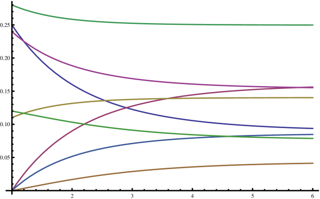
Figure 1. Frequencies of the human blood phenotypes for the initial distribution of genotypes 2$\cdot$OOhh + AOhh + 2$\cdot$ABHH

AH
BH
Oh Ah ABH OH
Bh ABh                                                                          Number of generations

We remark that it takes six human generations (around 200 years in the real time scale) for the phenotypes frequencies in this example to arrive at the 2% relative error neighborhood of their limit values.

4. Mathematica package for the analysis of the blood groups frequencies

While the evolutionary trajectory of any particular blood genotypes distribution is completely described by Theorem 1, the algebraic structure of the attracting invariant manifold of the dynamical system (1) is far from being clear. The analysis of its properties is a task of substantial computational complexity and was done by means of a package developed by the author and run under computer algebra system Mathematica 9.0. One of the core algorithms implemented in this package is as follows.

Algorithm 1.

Step 0  Define the list G with the 18 blood genotypes names OOhh, …, ABHH as formal symbolic algebraically independent variables. A population will from now on be identified with a linear form in the elements of G. Its mass is defined to be the sum of the coefficients of this linear form. Denote the space of all such forms by L(G).

Step 1  Define the blood genotypes inheritance matrix A to be the matrix of normalized (i.e., with mass 1) linear forms in the elements of G that encode the human blood genotypes inheritance rules.

Step 2  Define a bilinear map S acting on G$\times$G and with values in L(G) by means of the matrix A. With this map, the normalized next generation is computed as follows:

NextGeneration[population_]:=
Collect[Simplify[Expand[S[population,population]]/
mass[population]],G].

Step 3  Choose a population by specifying the values of some of the elements of the list G and imposing algebraic relations on the other.

Step 4  Find an algebraic parametrization of the attracting submanifold for the population in question by integrating the evolutionary equations.

Step 5  Eliminate the parameters and return the complete set of algebraic equations defining the attracting submanifold.

While there exist several computer programs for the numerical simulation of the evolution of recombination frequencies, the above algorithm appears to be new. The structure of invariant manifolds of a general multivariate map defined by a family of quadratic forms is far from being clear and presumably does not admit any algebraic description. The linearization of an evolutionary trajectory in a neighborhood of the equilibrium manifold has been given in [8].

Computer experiments with the Mathematica package reveal the following intrinsic property of the attracting manifold: it is given by a binomial ideal [14] generated by quadratic forms. A full list of these forms (many of them being algebraically dependent) contains 96 elements and the following shape: $x_{1}x_{10}=x_{4}x_{7},\,\,x_{1}x_{11}=x_{5}x_{7},\,\,x_{1}x_{12}=x_{6}x_{7},\,\,4x_{1}x_{13}=x_{7}^{2},4x_{1}x_{14}=x_{7}x_{8},\,\,x_{10}x_{14}=2x_{12}x_{13},$ $16x_{1}x_{15}=x_{8}^{2},\ldots,4x_{7}x_{9}=x_{8}^{2}.$

We now apply Algorithm 1 to investigate invariant manifolds of the polynomial dynamical system (1). We consider special cases of particularly simple distributions of blood genotypes in the initial population.

4.1. First blood group

Consider the special case of a population consisting of people with first blood group only (such as present day’s south american indians, see [9], p. 2189, Table 132-2). Assume that the population in question comprises $a$ people with the genotype OOhh, $b$ people with the genotype OOHh, and $c$ people with the genotype OOHH. Using the notation introduced above, we will denote such a population by $a\cdot{\rm OOhh}+b\cdot{\rm OOHh}+c\cdot{\rm OOHH}.$ Then, in accordance with the blood inheritance rules and their mathematical formulation (1), the blood genotypes distribution in the next generation will be

(8) $$(2a+b)^{2}\cdot{\rm OOhh}+2(2a+b)(b+2c)\cdot{\rm OOHh}+(b+2c)^{2}\cdot{\rm OOHH}$$

and it will remain unchanged in any subsequent generation. In other words, the variety parametrized for $(a,b,c)\in\hbox{\Bbb P}^{2}$ by

$$\left((2a+b)^{2},0,0,0,0,0,2(2a+b)(b+2c),\right.\left.0,0,0,0,0,(b+2c)^{2},0,0,0,0,0\right)\in\hbox{\Bbb P}^{17}$$

is an invariant manifold of the polynomial map (1) which moreover consists of fixed points of this map. The three nonzero equilibrium frequencies $x_{1},x_{7},x_{13}$ of the three genotypes in this example lie on the discriminant hypersurface $4x_{1}x_{13}=x_{7}^{2}.$

From now on we will be using the linear form notation for blood genotypes distributions since they allow one to avoid vectors with plenty of zeros.

4.2. Rh negative blood

Since Rh negative blood is a recessive trait, a population consisting of Rh negative people only can be represented in the following form:

$$p\cdot{\rm OOhh}+q\cdot{\rm AOhh}+r\cdot{\rm AAhh}+u\cdot{\rm BOhh}+v\cdot{\rm BBhh}+w\cdot{\rm ABhh}.$$

Such a distribution of blood genotypes will also stabilize already in the next generation. This new stable distribution is given by

(9) $$\begin{array}[]{c}(2p+q+u)^{2}\cdot{\rm OOhh}+2(2p+q+u)(q+2r+w)\cdot{\rm AOhh}+\\ (q+2r+w)^{2}\cdot{\rm AAhh}+2(2p+q+u)(u+2v+w)\cdot{\rm BOhh}+\\ (u+2v+w)^{2}\cdot{\rm BBhh}+2(q+2r+w)(u+2v+w)\cdot{\rm ABhh}.\phantom{-}\end{array}$$

For any $(p,q,r,u,v,w)\in\hbox{\Bbb P}^{5}$ the point (9) is another fixed point of the polynomial map (1). It is easily seen that the equilibrium frequencies satisfy the binomial relations $4x_{1}x_{3}=x_{2}^{2},\,\,4x_{1}x_{5}=x_{4}^{2},\,\,2x_{2}x_{5}=x_{4}x_{6},\,\,4x_{3}x_{5}=x_{6}^{2},\,\,2x_{1}x_{6}=x_{2}x_{4},\,\,x_{2}x_{6}=2x_{3}x_{4}.$

4.3. Evolution of the population $a\cdot$OOhh + $b\cdot$AAhh + $c\cdot$AAHH

Consider the population $P=a\cdot$OOhh + $b\cdot$AAhh + $c\cdot$AAHH. Here $a,b$ and $c$ are arbitrary positive numbers representing proportions of people with corresponding blood genotypes. Any real population is of course very far from having such a distribution of blood genotypes. We consider this example since it is essentially different from the previous ones and still allows one to explicitly compute the limit distribution of the blood genotypes.

Already the third generation of the population $P$ defined above will contain all nine genotypes that belong to the first or the second blood group. Using the Wolfram Mathematica 9.0 computer algebra system and a package for blood genotypes analysis we conclude that after sufficiently many generations the blood genotypes distribution in the population under study will be arbitrarily close to the limit distribution

(10) $$\begin{array}[]{r}a^{2}(a+b)^{2}\cdot{\rm OOhh}+2a(a+b)^{2}(b+c)\cdot{\rm AOhh}+(a+b)^{2}(b+c)^{2}\cdot{\rm AAhh}+\\ 2a^{2}(a+b)c\cdot{\rm OOHh}+4a(a+b)c(b+c)\cdot{\rm AOHh}+2(a+b)c(b+c)^{2}\cdot{\rm AAHh}+\\ a^{2}c^{2}\cdot{\rm OOHH}+2ac^{2}(b+c)\cdot{\rm AOHH}+c^{2}(b+c)^{2}\cdot{\rm AAHH}.\phantom{..}\end{array}$$

For any initial frequencies $a,b,c$ this blood genotypes distribution is invariant under the map $f.$ The nonzero equilibrium frequencies span the manifold defined by the binomial equations $4x_{1}x_{13}=x_{7}^{2},\,\,4x_{1}x_{14}=x_{7}x_{8},\ldots,$ $4x_{7}x_{9}=x_{8}^{2}.$

4.4. Blood with the same distribution of blood groups for all Rh genotypes

Statistics shows that in most populations blood group and Rh factor distributions do not correlate with each other [9, 2, 3, 4] . Since blood genotype (including all the information on homo- or heterozygosity of a person for blood group and Rh factor) is much more difficult to detect clinically than the dominating blood group and Rh factor, the corresponding statistics for their variations is not available. Yet, genetics of these traits suggests to consider them as statistically independent. In the present example, we investigate the blood genotypes dynamics of a population satisfying this additional assumption.

Such a population is completely determined by the two vectors $R=(a,b,c)\in\hbox{\Bbb P}^{2}$ and $G=(p,q,r,u,v,w)\in\hbox{\Bbb P}^{5}$ giving the numbers of people with Rh-factor variations (hh,Hh,HH) and the distribution of blood group variations (OO, AO, AA, BO, BB, AB) within every such set. With this notation, the 18-dimensional vector defining a population that satisfies the above assumption is given by the tensor product of the vectors $R$ and $G$ defined as follows: $R\otimes G=(ap,aq,ar,au,av,aw,bp,bq,br,bu,bv,bw,cp,cq,$ $cr,cu,cv,cw).$ Computation shows that the blood genotypes distribution of such a population will also stabilize in the next generation and the new stable distribution is the tensor product of the distributions (8) and (9):

$${\small\begin{array}[]{c}\left(\right.A(2p+q+u)^{2},\,\,2A(2p+q+u)(q+2r+w),\,\,A(q+2r+w)^{2},\,\,2A(2p+q+u)(u+2v+w),\\ A(u+2v+w)^{2},\,\,2A(q+2r+w)(u+2v+w),\,\,B(2p+q+u)^{2},\,\,2B(2p+q+u)(q+2r+w),\\ B(q+2r+w)^{2},\,\,2B(2p+q+u)(u+2v+w),\,\,B(u+2v+w)^{2},\,\,2B(q+2r+w)(u+2v+w),\\ C(2p+q+u)^{2},\,\,2C(2p+q+u)(q+2r+w),\,\,C(q+2r+w)^{2},\,\,2C(2p+q+u)(u+2v+w),\\ C(u+2v+w)^{2},\,\,2C(q+2r+w)(u+2v+w)\left.\right),\end{array}}$$

where $A=(2a+b)^{2},$ $B=2(2a+b)(b+2c),$ $C=(b+2c)^{2}.$

5. Back to real data

The image of the space of all blood genotypes distributions under the map (1) encoding the blood inheritance rules is six-dimensional. Thus the evolution of an 18-dimensional initial distribution is completely determined by its six parameters which can be chosen to be the frequencies of the fully homozygous blood genotypes. The initial distributions that evolve differently are those that do not differ by a vector in the kernel of the matrix (3).

It is classically known that the equilibrium phenotypes frequencies O,A and B of the 1st, 2nd and 3rd blood groups respectively satisfy the Bernstein algebraic relation [7, 5]  $1+\sqrt{{\rm O}}=\sqrt{{\rm A+O}}+\sqrt{{\rm B+O}}.$ This relation (together with O+A+B+AB=1) allows one to express e.g. the frequency of the 4th blood group as a function $F_{{\rm AB}}({\rm O,A})$ of the frequencies of the first two. Using statistical data available at www.bloodbook.com/world-abo.html where blood group distributions for 88 ethnicities of the world are collected, we find that the relative error of the estimate $F_{{\rm AB}}({\rm O,A})$ exceeds 30% in 11% of all cases. Also, this relative error is greater than 20% for 19% of all the observed blood groups phenotypes distributions. This suggests that many of the observed distributions do not lie on the Bernstein hypersurface (see Fig. 2) and therefore are not at the equilibrium and will necessarily evolve further.

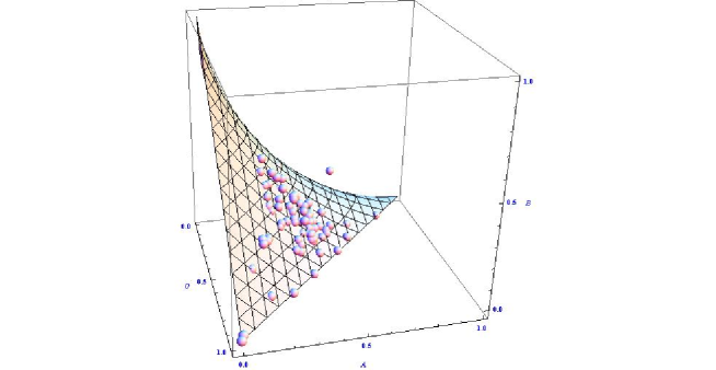
Figure 2. The Bernstein hypersurface $1+\sqrt{{\rm O}}=\sqrt{{\rm A+O}}+\sqrt{{\rm B+O}}$ and the observed distributions of blood groups frequencies in the world

The formula (2) gives a complete description of their evolutionary trajectories in the absence of evolutionary influences like meiosis, migration etc.

While extensive statistical data on blood phenotypes distributions in the various populations of the world is available at www.bloodbook.com/world-abo.html and similar sources, little is known about the human blood genotypes distributions. The reason for this is that a human’s blood genotype is much more difficult to detect clinically than her/his blood phenotype. However, to compute the expected blood phenotypes or genotypes distribution in the next generation, the present genotypes distribution must be known. This lack of statistical data does not allow us to directly apply Theorem 1 to a real population. Yet, the formula (2) shows which initial distributions evolve along the same trajectories as well as their rate of convergence towards the equilibrium.

References

- [1] Anstee, D.J., 2010. The relationship between blood groups and disease. Blood 115, 4635-4643.
- [2] Kang S.H. et al., 1997. Distribution of abo genotypes and allele frequencies in a korean population. Japanese Journal of Human Genetics 42, 331-335.
- [3] Ohashi J. et al., 2006. Polymorphisms in the ABO blood group gene in three populations in the New Georgia group of the Solomon Islands. Journal of Human Genetics 51, 407-411.
- [4] Sato T. et al., 2010. Polymorphisms and allele frequencies of the ABO blood group gene among the Jomon, Epi-Jomon and Okhotsk people in Hokkaido, northern Japan, revealed by ancient DNA analysis. Journal of Human Genetics 55, 691-696.
- [5] Novitski E., 1976. ABO blood groups and the Hardy-Weinberg equilibrium. Science 6, 478.
- [6] Bernstein, S.N., 1923. Principe de stationarite et generalisation de la loi de Mendel. C.R. Acad. Sci. Paris 177, 528-531.
- [7] Bernstein, F., 1930. Über die Erblichkeit der Blutgruppen. Zeitschrift für Induktive Abstammungs- und Vererbungslehre 54:1, 400-426.
- [8] Lyubich Y.I., 1971. Basic concepts and theorems on the evolutionary genetics of free populations. Russian Mathematical Surveys 26:5, 51-123.
- [9] Hoffman R. et al., 2012. Hematology: Basic Principles and Practice (6th ed.). Elsevier. ISBN 978-1-4377-2928-3.
- [10] Okada Y., Kamatani Y., 2012. Common genetic factors for hematological traits in Humans. Journal of Human Genetics 57, 161-169.
- [11] Reilly M., Szulkin R., 2007. Statistical analysis of donation-transfusion data with complex correlation. Stat. Med. 26:30, 5572-5585.
- [12] Bedford, E., Jonsson, M., 2000. Dynamics of regular polynomial endomorphisms of . Amer. J. Math. 122:1, 153-212.
- [13] Cantat S., Chambert-Loir A., Guedj V., 2010. Quelques aspects des systèmes dynamiques polynomiaux. (French) [ Some Aspects of Polynomial Dynamical Systems.] Panoramas et Synthèses [Panoramas and Syntheses], 30. Société Mathématique de France, Paris. x+341 pp. ISBN: 978-2-85629-338-6.
- [14] Eisenbud D., Sturmfels B., 1996. Binomial ideals. Duke Math. J. 84:1, 1-45.