Exploiting Data Representation for Fault Tolerance

Abstract

We explore the link between data representation and soft errors in dot products. We present an analytic model for the absolute error introduced should a soft error corrupt a bit in an IEEE-754 floating-point number. We show how this finding relates to the fundamental linear algebra concepts of normalization and matrix equilibration. We present a case study illustrating that the probability of experiencing a large error in a dot product is minimized when both vectors are normalized. Furthermore, when data is normalized we show that the absolute error is less than one or very large, which allows us to detect large errors. We demonstrate how this finding can be used by instrumenting the GMRES iterative solver. We count all possible errors that can be introduced through faults in arithmetic in the computationally intensive orthogonalization phase, and show that when scaling is used the absolute error can be bounded above by one.

I Introduction

In the field of high-end computing (HEC) the notion of reliability has tended to focus on keeping thousands of physical nodes operating cooperatively for extended periods of time. As chip manufacturing and power requirements continue to advance, soft errors are becoming more apparent [1]. This implies that reliability research must address the case that the machine does not crash, but that outputs during computation may be silently incorrect. There have been many studies into hardening numerical kernels against soft errors, that is the researchers attempt to preserve the illusion of a reliable machine by detecting and correcting all soft errors. We take a more analytical approach. Instead of focusing on detection/correction, we seek to study how the data operated on impacts the errors that we can observe given soft errors in data — called silent data corruption (SDC).

The driving motivation behind our work is the uncertainty surrounding the reliability of an exascale-class machine [2, 3, 4]. We attempt to avoid speculation over what hardware may be used in future (or present) HEC deployments, and instead analyze how a single soft error in an IEEE-754 floating-point number behaves. It has already been shown that existing and decommissioned HEC deployments have suffered from SDC [1, 5]. For the prior reasons, we seek to study the link between the data operated on and soft errors. We intentionally perform our research subject to the IEEE 754 specification, which we believe will be used regardless of the architecture. We also restrict our analysis to single bit flips. This gives us a base line from which to draw higher-level conclusions related to multiple bit flips, and lets us isolate the impact of a bit flip.

IEEE 754 both defines the binary representation of data, and bounds the rounding error committed by arithmetic operations. This work focuses on data representation. The effects of rounding error on numerical algorithms, including those studied in this paper, have been extensively studied; see e.g., [6]. However, these results generally only apply to small errors, such as those resulting from rounding. Bit flips can be huge and thus require different methods of analysis, like those presented in this paper.

We present the following contributions:

• We model single bit upsets in IEEE-754 scalars analytically, and extend this modeling to dot products.

• We demonstrate both experimentally (via Monte Carlo sampling) and analytically that dot products performed on normalized numbers have a significantly lower probability of experiencing large error than dot products with values of varying magnitudes.

• We relate our finding that normalized vectors minimize absolute error to matrix equilibration, and correlate this finding to two highly used numerical kernels (Gram-Schmidt orthogonalization and the Arnoldi process).

• We demonstrate the utility of our finding by instrumenting the Generalized Minimum Residual Method (GMRES). We show that for the dot product intensive orthogonalization kernel, we can restrict errors arising from single bit upsets to being less than one, or being very large and easily detected.

• We articulate how studying single bit flips enables us to draw conclusions about multiple bit upsets.

II Related Work

Researchers have approached the problem of SDC in numerical algorithms in various ways. Many take the approach of treating an algorithm as a black box and observing the behavior of these codes when run with soft errors injected. Recently, [7, 8] analyzed the behavior of various Krylov methods and observed the variance in iteration count based on the data structure that experiences the bit flip. Shantharam et al. [9] analyzed how bit flips in a sparse matrix-vector multiply (SpMV) impact the $L^{2}$ norm and observe the error as CG is run. Bronevetsky et al. [10, 11] analyzed several iterative methods documenting the impact of randomly injected bit flips into specific data structures in the algorithms and evaluated several detection/correction schemes in terms of overhead and accuracy. Exemplifying the concept of black-box analysis, [12] presents BIFIT for characterizing applications based on their vulnerability to bit flips. Rather than focusing on how to preserve the illusion of a reliable machine or devising a scheme to inject soft errors, we investigate an avenue mostly ignored, which is how the data in the algorithm can be used to mitigate the impact of a bit flip.

Hoemmen and Heroux proposed a radically different approach. Rather than attempt to detect and correct soft errors, they use a “selective reliability” programming model to make the algorithm converge through soft errors [13]. Sao and Vuduc showed that reliably restarting iterative solvers enables convergence in the presence of soft errors [14]. In the same vein, Elliott et al. showed that bounding the error introduced in the orthogonalization phase of GMRES lets FT-GMRES converge with minimal impact on time to solution [15]. Boley et al. apply backward error analysis to linear systems, in order to distinguish small error due to rounding from inacceptably large error due to transient hardware faults [16]. In general, our work complements this line of research. While Hoemmen and Sao have investigated algorithms that can converge through error, we show that in certain numerical kernels, the data itself can have a “bounding” effect. For example, coupled with [15], we improve the likelihood that errors fall within the derived bound.

Algorithm-based fault tolerance (ABFT) provides an approach to detect (and optionally correct) faults, which comes at the cost of increased memory consumption and reduced performance [17, 18]. The ABFT work by Huang et al. [17] was proven by Anfinson et al. [19] to work for several matrix operations, and the checksum relationship in the input checksum matrices is preserved at the end of the computation. Consequently, by verifying this checksum relationship in the final computation results, errors can be detected at the end of the computation. Recent work has looked at extending ABFT to additional matrix factorization algorithms [18] and as an alternative to traditional checkpoint/restart techniques for tolerating fail-stop failures [20, 21, 22].

Costs in terms of extra memory and computation required for ABFT may be amortized for dense linear algebra, and such overheads have been analyzed by many (e.g., [23, 24, 25]). Algorithms must be manually redesigned for ABFT support by accounting for numerical properties (e.g., invariants). A more fundamental problem is that traditional checksums and error-correcting codes do not suit floating-point computations well [16]. Such computations naturally commit rounding error, which exact (bitwise) codes forbid. Inexact codes (that use floating-point sums) can be sensitive to rounding error, and commit it themselves. It is possible that more expensive recovery and significantly more redundant storage could help [26]. However, works like [13, 14, 15, 16] suggest that correcting faults might not be necessary, if their effects on the algorithm are detectable and bounded. In general, this paper favors “opening up the black box” and understanding the effects of soft error on algorithms, rather than trying to detect and correct all such errors before they affect algorithms’ behavior.

III Project Overview

To explore the relation between data representation and soft errors, we first construct an analytic model of a soft error in an IEEE-754 floating-point scalar, and then extend this to a dot product. We uncover through analysis that the binary pattern of the exponent can be exploited for fault tolerance. We show this graphically via a case study using Monte Carlo sampling of random vectors, and then extend the idea of data scaling to matrices by using sparse matrix equilibration. To demonstrate the feasibly and utility of our work we analyze the GMRES algorithm and instrument the computationally intensive orthogonalization phase. We count the possible absolute errors that can be introduced via a bit flip in a dot product, and show that scaling data lowers the likelihood of observing large, undetectable errors.

This paper is organized as follows:

1. In Section IV, we construct an analytic model of the absolute error for single bit upsets in IEEE-754 floating-point numbers.

2. In Section V, we extend our model of faults in IEEE-754 scalars to vectors of arbitrary values, and present examples of how data scaling impacts the binary representation and absolute error we can observe.

3. In Section VI, we perform a case study using Monte Carlo sampling of 10,404,000,000 random vectors of various magnitudes, and graphically show how the error is minimized when operating on values less than 1.

4. In Section VII, we link data scaling to sparse matrix equilibration, and instrument and evaluate the impact of a soft error in the computationally intensive orthogonalization phase of GMRES.

IV Fault Model

The premise of our work is that a silent, transient bit flip impacts data. Before we can perform any analysis or experimental work, we must define how such a bit flip would impact an algorithm, and how we enforce that the bit flip was transient. To achieve this goal, we build our model around the basic concept that when an algorithm uses data, this translates into some set of operations being performed on the data. Should a bit flip perturb our data, some operation will use a corrupt value, rather than the correct value. The output of this single operation will then contain a tainted value, and this tainted value could cause the solution to be incorrect. Note that a transient bit flip may cause a persistent error in the output depending on how the value is used.

A side benefit of an operation-centric model is that we naturally avoid a pitfall to which arbitrary memory fault injection succumbs, namely that if a bit flip impacts data (or memory) that is never used (read) then this fault cannot lead to a failure. Our fault model allows a bit flip to perturb the input to an operation performed on the data, while not persistently tainting the storage of the inputs. This mimics how a transient bit flip would manifest itself, e.g., during ALU activities. As a result, the data that experiences the bit flip need not show signs that it was perturbed. This model allows us to observe the impact of transient flips on the inputs, which results in sticky or persistent error in the result. We then utilize mathematical analysis to model how this persistent error propagates through the algorithm.

IV-A Fault Characterization via Semantic Analysis

To derive a fault model we must first understand what a fault is. Since floating-point numbers approximate real numbers and most numerical algorithms use real numbers, we start from the definition of a real-valued scalar $\gamma\in\mathbb{R}$. The range of possible values that $\gamma$ can take is

$$\gamma\in[-\infty,+\infty].$$

We assume that the IEEE-754 specification for double-precision numbers, called Binary64, is used to represent these numbers. This means that $\gamma$ can take a fixed set of numeric values, and these values lie in the range

$$\gamma\in[-1.80\times 10^{308},+1.80\times 10^{308}],$$

or using base two for the exponent

$$\gamma\in[-1.\bar{9}\times 2^{1023},+1.\bar{9}\times 2^{1023}],$$

where $1.\bar{9}$ indicates the largest possible fractional component, and $1.0$ indicates the smallest fractional component. A more informative range is that of $\left|\gamma\right|$, excluding $0$ and denormalized numbers,

$$\left|\gamma\right|\in[2.23\times 10^{-308},1.80\times 10^{308}],$$ (1)

and in semi base two

$$\left|\gamma\right|\in[1.0\times 2^{-1022},1.\bar{9}\times 2^{1023}].$$ (2)

To approximate real numbers, Binary64 uses 64 bits, of which 11 are devoted to the exponent, 52 for the fractional component (we refer to as the mantissa), and one bit for the sign. Figure 1 shows how these bits are laid out.

Figure 1: Graphical representation of data layout in the IEEE-754 Binary64 specification.

In addition to numeric values, Binary64 includes two non-numeric values, Not-a-Number (NaN) and Infinity (Inf), which may be signed to account for infinity and values that result in undefined operations, e.g., division by zero. The range of values in Equations (1) and (2) is not continuous and has non-uniform gaps due to the discrete precision, which is a consequence of having a fixed number of bits in the fractional component.

We can further discretize the range of possible values by recognizing that there is a finite number of exponents that are possible given IEEE-754 double precision, e.g.,

$$\gamma\in\{ 0,\pm\mathrm{Inf},\pm\mathrm{NaN},\pm 2^{-1022}\times 1.x,\pm 2^{-1021}\times 1.x,$$

$$\dotsc,\pm 2^{0}\times 1.x,\dotsc,\pm 2^{1023}\times 1.x\},$$

where $1.x$ indicates some fractional component.

Analytically, this is expressed as

$$\gamma=(-1)^{sign}\left(1+\sum\limits_{i=0}^{51}b_{i}2^{i-52}\right)\times 2^{e-1023},$$ (3)

for IEEE-754 Binary64. Note, the specification does not include a sign bit for the exponent. Rather, IEEE floating point numbers utilize a bias to allow the exponent to be stored without a sign bit, which we will later exploit for fault-resilience. Another important characteristic that stems from the general approach of expressing numbers in exponential notation is that we can characterize numbers by their order of magnitude. Of particular interest is the following relation:

$$|2^{-1022}| \leq|2^{-1022}\times 1.x|$$

$$<|2^{-1021}| \leq|2^{-1021}\times 1.x|<\dots$$

$$<|2^{0}| \leq|2^{0}\times 1.x|<\dots$$

$$<|2^{1023}| \leq|2^{1023}\times 1.x|.$$ (4)

This means that we can use the next order of magnitude as an upper bound for errors in the fractional component of a number — which is practically achieved by incrementing the exponent or multiplying by two. We can also analytically model the number of fractional bits that could contribute an error larger than some tolerance, since the error that could arise from each mantissa bit is relative to the exponent of the number. This final step is necessary since the fractional term can take values in the range $[1,2)$, where the left parenthesis indicates that $2$ is not a member of this interval. We can also characterize the error that a perturbed sign bit can contribute, and, like the fractional component, this error is relative to the exponent of the number. Suppose the sign is perturbed in a scalar $\gamma$, then we have $\tilde{\gamma}=-\gamma$, the absolute error is $|\gamma-\tilde{\gamma}|=|\gamma-(-\gamma)|=2\gamma$. This means we can bound the error from a sign bit perturbation by incrementing the exponent of the resulting value.

In summary, we have demonstrated that errors in IEEE-754 floating point numbers can be characterized using the exponent of the numbers. This property allows us to reduce the number of bits we need to consider in a fault model, since we know that a large number of errors are bounded by the relatively small set of possible exponents.

IV-B Fault Characteristics of Perturbed Exponents

In the context of IEEE-754 double precision numbers and silent data corruption, we do not model the exponents directly. Instead, we model the biased exponents, as they are the interesting portion of the data that allows us to characterize the errors that the majority of the bits present in the data can produce. For instance, in double precision data we can characterize the errors from 53 of the 64 bits using our approach. This type of fault-characterization is impossible if bit flips are injected randomly into the data’s memory, as that approach loses the semantic information that is implicitly present in the data.

The Binary64 specification does not store exponents directly, instead it uses a bias of $1023$. From § IV-A this means we can characterize all faults in double precision data by analyzing perturbations to the possible biased exponents

$$\{0,1,2,\dotsc,1023,\dotsc,2046\}.$$

Note that zero is not a biased exponent and has special meaning. In IEEE-754, a zero pattern in the exponent with zeros in the mantissa is used to represent the scalar zero, while a non-zero pattern in the mantissa is used to represent subnormal numbers. We also assume the user does not perform computation on the two non-numeric values NaN and Inf, which are represented using the biased exponent $2047$ (all ones). We do include zero in our analysis because it is a valid real number.

Since we are concerned with bit perturbations in the exponent, we express the biased exponents in their binary form, e.g., 11-bit unsigned integers presented in binary.

$$\begin{array}[]{ccccc}\left\{\!\!\!\begin{array}[]{c}2^{-1}\\ 2^{0}\\ 2^{1}\\ \end{array}\!\!\!\right\}&\Rightarrow&\left\{\!\!\!\begin{array}[]{c}1022\\ 1023\\ 1024\\ \end{array}\!\!\!\right\}&\Rightarrow&\left\{\!\!\!\begin{array}[]{c}01111111110\\ 01111111111\\ 10000000000\\ \end{array}\!\!\!\right\}\\ \mathrm{Exponent}&&\mathrm{Biased}&&\mathrm{Storage}\end{array}$$

Figure 2: Relation of exponent, IEEE-754 double precision bias, and what data are actually stored.

We can further expand Figure 2 to show the potential change to the original exponent should a bit flip occur, which will form the basis for our fault model and analytic models.

In the context of bit flips, we can view a bit flip as adding or subtracting from the biased exponent, which in turn translates to multiplying or dividing the number by some power of two. We model the impact of a bit flip in the exponent as the original scalar being magnified or minimized by a specific power of two. We illustrate this in Figure 3, where reading left-to-right, we have some initial exponent, which is represented using a bias of $1023$. The biased exponent translates to a discrete binary pattern. We consider all single bit flips in this binary pattern and compute the actual perturbed exponent. Note, that the perturbation can be modeled independent of the original exponent.

$$\begin{array}[]{ccccccccc}2^{-1}&\!\!\Rightarrow\!\!&1022&\!\!\Rightarrow\!\!&01111111110&\!\!\!\!\Rightarrow\!\!\!\!&\left\{\!\!\!\begin{array}[]{c}01111111111\\ 01111111100\\ 01111111010\\ 01111110110\\ 01111101110\\ 01111011110\\ 01110111110\\ 01101111110\\ 01011111110\\ 00111111110\\ 11111111110\end{array}\!\!\!\right\}&\!\!\!\!\Rightarrow\!\!&\left\{\!\!\!\begin{array}[]{c}2^{0}=2^{-1}\times 2^{+1}\\ 2^{-3}=2^{-1}\times 2^{-2}\\ 2^{-5}=2^{-1}\times 2^{-4}\\ 2^{-9}=2^{-1}\times 2^{-8}\\ 2^{-17}=2^{-1}\times 2^{-16}\\ 2^{-33}=2^{-1}\times 2^{-32}\\ 2^{-65}=2^{-1}\times 2^{-64}\\ 2^{-129}=2^{-1}\times 2^{-128}\\ 2^{-257}=2^{-1}\times 2^{-256}\\ 2^{-513}=2^{-1}\times 2^{-512}\\ 2^{1023}=2^{-1}\times 2^{1024}\\ \end{array}\!\!\!\right\}\end{array}$$

$$\begin{array}[]{ccccccccc}2^{0}&\!\!\Rightarrow\!\!&1023&\!\!\Rightarrow\!\!&01111111111&\!\!\!\!\Rightarrow&\left\{\!\!\!\begin{array}[]{c}01111111110\\ 01111111101\\ \vdots\\ 00111111111\\ 11111111111\end{array}\!\!\!\right\}&\!\!\!\!\Rightarrow\!\!&\left\{\!\!\!\begin{array}[]{c}2^{-1}=2^{0}\times 2^{-1}\\ 2^{-2}=2^{0}\times 2^{-2}\\ \vdots\\ 2^{-512}=2^{0}\times 2^{-512\phantom{n}}\\ 2^{1024}=\mathrm{Inf~{}or~{}NaN}\end{array}\!\!\!\right\}\end{array}$$

$$\begin{array}[]{ccccccccc}2^{1}&\!\!\Rightarrow\!\!&1024&\!\!\Rightarrow\!\!&10000000000&\!\!\!\!\Rightarrow\!&\left\{\!\!\!\begin{array}[]{c}10000000001\\ 10000000010\\ \vdots\\ 11000000000\\ 00000000000\end{array}\!\!\!\right\}&\!\!\!\!\Rightarrow\!\!\!&\left\{\!\!\!\begin{array}[]{c}2^{2}=2^{1}\times 2^{+1}\\ 2^{3}=2^{1}\times 2^{+2}\\ \vdots\\ 2^{513}=2^{1}\times 2^{+512\phantom{nm}}\\ \mathrm{Zero~{}or~{}Subnormal}\end{array}\!\!\!\right\}\\ \lx@intercol\hfil\underbrace{\hskip 130.0pt}_{\text{Unperturbed Data}}\hfil\lx@intercol&&\underbrace{\hskip 50.0pt}_{\text{Possible Binary}}&&\underbrace{\hskip 25.0pt}_{\text{Result}}\phantom{=2^{1}}\underbrace{\hskip 30.0pt}_{\text{Perturbation}}\end{array}$$

Figure 3: Examples of how a bit flip can impact an exponent represented using the IEEE-754 Binary64 specification.

By characterizing the error introduced, we recognize that all mantissa bit flips introduce error that has the same exponent as the original number, and a sign bit flip introduces error that is only one order of magnitude larger than the original number. Furthermore, the exponent bits can either introduce large error, or a bit flip introduces error roughly equivalent to the order of magnitude of the original number.

Suppose we can enforce that all numbers used in calculations are less than $1.0$, then we know that the majority of the bits will produce error that is also less than one, since 51 of the total 52 mantissa bits will contribute an error less than $1.0$. We also see that some of the exponent bits have the potential to contribute an error less than $1.0$, which indicates if we can enforce or assume some properties of the data used in the calculations e.g., data less than one, then we can greatly increase the likelihood that a bit flip introduces an error no greater than $1.0$. This phenomena is shown in Figure 3, where we show empirically that numbers with exponent $2^{0}$ introduce a small error compared to the errors introduced with the exponent $2^{1}$.

In summary, the exponent characterizes the error introduced by the sign or mantissa should a bit flip occur. As discussed in § IV-A and analytically presented in Eq. (4), we are able to relate bit upsets to numerical error in terms of the exponent of the original number. Table I summarizes these analytical bounds for a bit upset in a scalar and highlights the change in order of magnitude. Now that we have characterized a fault in a scalar, we will present a fault model centered around operations on scalars assuming one will be perturbed.

TABLE I: Bit flip absolute error for a scalar $\lambda$ represented using IEEE-754 double precision, with $\lambda~{}=~{}\lambda_{\mathrm{exp}}~{}\times~{}\lambda_{\mathrm{frac}}$. Where $\lambda_{\mathrm{exp}}$ is the exponent $2^{x}$, and $\lambda_{\mathrm{frac}}$ is the fractional component.

Bit Location	Absolute Error		Bit Range	$\Delta$ Order†
	Scalar: $\left|\lambda-\tilde{\lambda}\right|$	Multiplication: $\left|\alpha\beta-\tilde{\alpha}\beta\right|$
Mantissa	$\left|\lambda_{\mathrm{exp}}(1+2^{j-52})\right|$	$\left|\alpha_{\mathrm{exp}}(1+2^{j-52})\beta\right|$	for $j=0,\dotsc,51$	$0$
Exponent1→0	$\left|\lambda(1-2^{-2^{j}})\right|$	$\left|\alpha\beta(1-2^{-2^{j}})\right|$	for $j=0,\dotsc,10$ and ${bit}_{j+52}=1$	$-2^{j}$
Exponent0→1	$\left|\lambda(1-2^{2^{j}})\right|$	$\left|\alpha\beta(1-2^{2^{j}})\right|$	for $j=0,\dotsc,10$ and ${bit}_{j+52}=0$	$+2^{j}$
Sign	$\left|2\lambda\right|$	$\left|2\alpha\beta\right|$		$1$
† The change in order of magnitude.

IV-C Operation Centric Fault Model

This work distinguishes itself from related work in the field of silent data corruption by developing a fault model that is not based on perturbing arbitrary memory locations. We seek a fault model and experimental methodology that expresses all possible errors, and not the expected error, which is what is obtained through random sampling.

IV-C1 Fault Model for Dot Products

We now describe a realization of our fault model that describes the error that could be injected if an operation in a dot product experiences a single bit upset. We choose the dot product because it is a common operation, and because we will use this model in § VII to model the worst-case errors that could be injected into a phase of the GMRES algorithm.

Given two real-valued $n$-dimensional vectors $\boldsymbol{\mathbf{a}},\boldsymbol{\mathbf{b}}\in\mathbb{R}^{n}$, the dot product is defined as

$$c=\sum\limits_{i=1}^{n}c_{i},~{}~{}\text{where}~{}~{}c_{i}=a_{i}b_{i}.$$ (5)

If we allow a single bit flip to impact the $i$-th element of the dot product, then we have a perturbed solution $\tilde{c}$, which is the result of a perturbation to either $a_{i}$, $b_{i}$, or $c_{i}$. In the context of our fault model, this captures a bit upset impacting the inputs to the multiplication operator, and it captures a bit upset in the intermediate value, $c_{i}$, which is the input to the addition operator.

Using Table I, we have all of the tools necessary to compose an absolute error model for a dot product, i.e., addition is modeled by a fault in a scalar $\left|\alpha+\beta-(\tilde{\alpha}+\beta)\right|=\left|\alpha-\tilde{\alpha}\right|$. The potential change in order of magnitude is paramount. Consider an exponent flip from $1\to 0$. These types of exponent bit flips produce an error that is bounded above by the original magnitude of the result, which can be viewed as “zeroing out” the term if a perturbation occurs. Similar to a perturbed scalar, the mantissa can contribute either no change in the order of magnitude, or in the worst case a bit flip causes a carry, which will increment the order of magnitude by one. The order of magnitude for a sign bit flip is exactly the same as that of a perturbed scalar, which introduces an error one order of magnitude larger than the result. These error models can be thought of as the largest additive error that we can inject into a dot product from a bit flip, e.g.,

$$\tilde{c}=\sum\limits_{i=1}^{n}a_{i}b_{i}+(\mathrm{error~{}term}).$$ (6)

In summary, we have composed analytic models for the the absolute error that could be introduced into a dot product. Our models are initially constructed from the IEEE-754 Binary64 model, which we extended to express how a bit upset impacts a singular double precision scalar. We then composed a model for the multiplication operator, and analytically expressed the absolute error. Using the absolute error, we have a model that explains how wrong a dot product can be, assuming a bit flip in one of the input vectors or in an intermediate value. Next, we refine these models to construct strict upper bounds on the error introduced by a bit flip in a dot product.

IV-C2 Error Bounds for a Bit Flip in a Dot Product

The models presented in Table I make no assumptions about the bits present in the mantissa of the operands. This is problematic if we want to consider all possible errors that could be introduced into a dot product. To account for the mantissa, and to create strict upper bounds on the error, we will use the relation presented in Eq. 4. From this relation, we know that $\alpha\beta<2^{\alpha_{\mathrm{exponent}}+1}2^{\beta_{\mathrm{exponent}}+1}$. We can write this as

$$\alpha\beta<4\alpha_{\mathrm{exp}}\beta_{\mathrm{exp}},$$ (7)

where $\alpha_{\mathrm{exp}}=2^{\alpha_{\mathrm{exponent}}}$. Using Eq (7), we are able to account for the mantissa bits, but we can also show that a bit flip in the sign is bounded by Eq. (7). The sign bit introduces an absolute error equivalent to incrementing the exponent of the result

$$\alpha\beta<2\alpha\beta<4\alpha_{\mathrm{exp}}\beta_{\mathrm{exp}},$$ (8)

where $2\alpha\beta$ is the potential error introduced should the sign bit be perturbed, which must be smaller than the bound constructed for the mantissa.

By utilizing Eq. (7), we are able to account for all possible mantissas and their potential faults, as well as a perturbation to the sign bit. We will now discuss how to use this model to understand the relationship between the data in an algorithm and the distribution of potential errors that could occur should a bit flip in the data.

V Fault Model Evaluation

In Section IV we proposed analytic models for errors should a bit flip occur in IEEE-754 double precision data. We now illustrate how data can impact the size of errors that a bit flip can create. Consider the following sample vectors

$$\boldsymbol{\mathbf{u}}_{\mathrm{small}}=\left[\!\!\!\begin{array}[]{c}0.5\\ 0.25\end{array}\!\!\!\right],~{} \boldsymbol{\mathbf{v}}_{\mathrm{small}}=\left[\!\!\!\begin{array}[]{c}0.25\\ 0.5\end{array}\!\!\!\right],~{}\text{and}~{}$$

$$\boldsymbol{\mathbf{u}}_{\mathrm{large}}=\left[\!\!\!\begin{array}[]{c}2\\ 4\end{array}\!\!\!\right],~{} \boldsymbol{\mathbf{v}}_{\mathrm{large}}=\left[\!\!\!\begin{array}[]{c}4\\ 2\end{array}\!\!\!\right].$$

If we compute the dot product $\lambda=\boldsymbol{\mathbf{u}}_{\mathrm{large}}\cdot\boldsymbol{\mathbf{v}}_{\mathrm{large}}$, we have a finite number of potential errors should a bit flip in the data of $\boldsymbol{\mathbf{u}}_{\mathrm{large}},\boldsymbol{\mathbf{v}}_{\mathrm{large}}$, or in an intermediate value in the summation. We can experience either $\tilde{2}\times 4+4\times 2$, $2\times\tilde{4}+4\times 2$, or $\tilde{8}+8$. We have previously shown what $\tilde{2}$ can be (in Figure 3), but for clarity we will state what the perturbed values could be (in Figure 4).

$$\tilde{2}=\left\{\!\!\!\begin{array}[]{c}2^{2}\\ 2^{3}\\ 2^{5}\\ 2^{9}\\ 2^{17}\\ 2^{33}\\ 2^{65}\\ 2^{129}\\ 2^{257}\\ 2^{513}\\ \mathrm{Zero}\\ \end{array}\!\!\!\right\},\quad\tilde{4}=\left\{\!\!\!\begin{array}[]{c}2^{1}\\ 2^{4}\\ 2^{6}\\ 2^{10}\\ 2^{18}\\ 2^{34}\\ 2^{66}\\ 2^{130}\\ 2^{258}\\ 2^{514}\\ 2^{-1020}\\ \end{array}\!\!\!\right\},\quad\tilde{8}=\left\{\!\!\!\begin{array}[]{c}2^{4}\\ 2^{1}\\ 2^{7}\\ 2^{11}\\ 2^{19}\\ 2^{35}\\ 2^{67}\\ 2^{131}\\ 2^{259}\\ 2^{515}\\ 2^{-1018}\\ \end{array}\!\!\!\right\}$$

Figure 4: Example of perturbed values for large numbers.

By inspection it is clear that substituting any of the above perturbed scalars into the dot product will produce an absolute error greater than one in all cases, and in the event one chooses to substitute the near zero perturbed values, the absolute error of the dot product still has magnitude $8$, e.g., $\left|16-(0+8)\right|$.

Alternatively, consider the vectors $\boldsymbol{\mathbf{u}}_{\mathrm{small}}$ and $\boldsymbol{\mathbf{v}}_{\mathrm{small}}$. If we compute the dot product, $\lambda=\boldsymbol{\mathbf{u}}_{\mathrm{small}}\cdot\boldsymbol{\mathbf{v}}_{\mathrm{small}}=0.25$. Then we have possible values to perturb: $\widetilde{0.5}$, $\widetilde{0.25}$, and $\widetilde{0.125}$. We construct these from our model of a perturbed scalar, and present the perturbed variants in Figure 5.

$$\widetilde{0.5}=\left\{\!\!\!\begin{array}[]{c}2^{0}\\ 2^{-3}\\ 2^{-5}\\ 2^{-9}\\ 2^{-17}\\ 2^{-33}\\ 2^{-65}\\ 2^{-129}\\ 2^{-257}\\ 2^{-513}\\ 2^{1022}\\ \end{array}\!\!\!\right\},\widetilde{0.25}=\left\{\!\!\!\begin{array}[]{c}2^{-3}\\ 2^{0}\\ 2^{-6}\\ 2^{-10}\\ 2^{-18}\\ 2^{-34}\\ 2^{-66}\\ 2^{-130}\\ 2^{-258}\\ 2^{-514}\\ 2^{1019}\\ \end{array}\!\!\!\right\},\widetilde{0.125}=\left\{\!\!\!\begin{array}[]{c}2^{-2}\\ 2^{-1}\\ 2^{-7}\\ 2^{-11}\\ 2^{-19}\\ 2^{-35}\\ 2^{-67}\\ 2^{-131}\\ 2^{-259}\\ 2^{-515}\\ 2^{1017}\\ \end{array}\!\!\!\right\}$$

Figure 5: Example of perturbed values for small numbers.

By inspection, $\widetilde{0.5}$ can contribute an absolute error to the dot product larger than one only once, e.g., $\left|0.25-(2^{1022}\times 0.25+0.125)\right|$. Likewise, $\widetilde{0.25}$ and $\widetilde{0.125}$ can perturb the result of the dot product with error greater than one only once, and for all 3 cases the perturbation will change the result by hundreds of orders of magnitude.

Returning to Figure 3 explains what causes bit flips in the exponent to produce either a majority of large or small errors. The binary pattern of the stored biased exponent contains predominantly zeros for numbers greater than one, and predominantly ones for numbers less than one.

One could also obtain primarily ones in the exponent as you approach the extrema of the biased exponents, i.e., numbers larger than $2^{512}$. In this case, the biased exponent does contain many ones, however, because the number is sufficiently large, i.e., the absolute error will remain considerably large. This is because if one “zeroes out” a perturbed element in the dot product, the error is proportional to the magnitude of the result.

V-A Faults in the Mantissa or Sign

The error generated by the mantissa or sign bits is relative to the exponent of the number that the flip occurred in. If the exponent is larger than one, then clearly the mantissa or sign bits can generate an error larger than one. Alternatively, if the values all are less than one, then mantissa errors will produce errors less than one because $2^{-1}\times 1.x\leq 2^{0}$. The errors from the sign bit cannot exceed $2$ since $2\times 2^{-1}\times 1.x<2^{1}$.

It is reasonable to consider that the mantissa generates a carry, as discussed in § IV-C2. To account for this we construct a strict upper bound by incrementing the exponent of each element of the vectors analyzed, similar to Eq. (7). For example,

$$\boldsymbol{\mathbf{u}}_{\mathrm{original}}=\left[\!\!\!\begin{array}[]{c}2.12332\\ 1.24568\end{array}\!\!\!\right]~{}\Rightarrow~{}\boldsymbol{\mathbf{u}}_{\mathrm{upper~{}bound}}=\left[\!\!\!\begin{array}[]{c}4\\ 2\end{array}\!\!\!\right].$$ (9)

We then can evaluate our models on these vectors to determine a strict upper bound on the errors we can experience in a dot product.

V-B Modeling Large Vectors

We have shown how to exhaustively examine each element in a vector, and from this analysis we can determine precisely which absolute errors we could experience. Given large vectors, where the dimension $n$ may have millions or billions of elements, exhaustively searching each element would be time consuming, but it would also be a waste of time. As stated previously, there is a discrete number of exponents supported by the IEEE-754 Binary64 specification. As we have previously shown, the exponent characterizes the faults we can observe, so we only need to consider the 2046 possible biased exponents and the special case of zero. The perturbations that are possible can be determined independent of concrete data values, e.g., we can precompute the perturbations and absolute error because we know the relation stated in Eq. (4) and Eq. (7).

To analyze arbitrarily large vectors, we construct a lookup table for the absolute error in whatever operation we choose to model (we have chosen products and addition). The table size is $2047\times 2047$, and allows us to consider the error introduced by performing an operation on two exponents, which will map to a unique $ij$ location.

For example, consider the vectors

$$\boldsymbol{\mathbf{u}}=\left[\!\!\!\begin{array}[]{c}1.0\\ 1.2\\ 8.0\\ 0.125\\ \end{array}\!\!\!\right],~{}\text{and}~{}\boldsymbol{\mathbf{v}}=\left[\!\!\!\begin{array}[]{c}0.125\\ 0.125001\\ 0.125002\\ 1.0\\ \end{array}\!\!\!\right].$$ (10)

We first extract the biased exponents from the vectors

$$\boldsymbol{\mathbf{u}}\Rightarrow\boldsymbol{\mathbf{u}}_{\mathrm{exponent}}=\left[\!\!\!\begin{array}[]{c}2^{0}\times 1.0\\ 2^{0}\times 1.x\\ 2^{3}\times 1.0\\ 2^{-3}\times 1.0\\ \end{array}\!\!\!\right]\Rightarrow\boldsymbol{\mathbf{u}}_{\mathrm{biased}}=\left[\!\!\!\begin{array}[]{c}1023\\ 1023\\ 1026\\ 1020\\ \end{array}\!\!\!\right]$$ (11)

Now, we determine an interval of possible values, and account for the mantissa values that may have been truncated

$$u_{i}\in[1020,1026]\subseteq[1020,1027]~{}\text{for}~{}i=1,\dotsc,4.$$ (12)

The range of biased exponents $[1020,1027]$ will contain all possible values that the original vector contained, and include one value that was larger than any in the vector, the number corresponding to the biased exponent $1027$. Similarly, we can compute the interval for $\boldsymbol{\mathbf{v}}$

$$\boldsymbol{\mathbf{v}}=\left[\!\!\!\begin{array}[]{c}0.125\\ 0.125001\\ 0.125002\\ 0.25\\ \end{array}\!\!\!\right]\!\!\Rightarrow\!\!\left[\!\!\!\begin{array}[]{c}2^{-3}\times 1.0\\ 2^{-3}\times 1.x\\ 2^{-3}\times 1.x\\ 2^{-2}\times 1.0\\ \end{array}\!\!\!\right]\!\!\Rightarrow\!\!\left[\!\!\!\begin{array}[]{c}1020\\ 1020\\ 1020\\ 1021\\ \end{array}\!\!\!\right],$$ (13)

which leads to the interval we consider errors

$$v_{i}\in[1020,1021]\subseteq[1020,1022]~{}\text{for}~{}i=1,\dotsc,4.$$ (14)

To allow us to analyze intervals efficiently, we create a lookup table, where each entry computes the relevant perturbations and absolute errors for the operations being modeled. In the case of multiplication, the table has symmetry because multiplication is commutative. In practice, computing the full table ($0,\dotsc,2046$) is simple and allows one to model errors for arbitrary vectors.

A caveat of the above approach is that we must know the range of values that the vector contains. This can be achieved by directly computing the min and max values for each vector. Alternatively, an approximate range can be determined if the “length” of the vector is known, e.g., the two-norm or if we know that the data is normalized, i.e., the two-norm is one. One weakness to the proposed approach is that we do not consider a flip in the accumulating sum, which we have left to future work. We also leave to future work analysis that shows how many of these modeled errors lie within the rounding error bound for pairwise sums.

V-C Summary

We have shown that the range of values used in the dot product has a direct impact on the size of the errors that can be observed. A general rule in floating point algorithms has been to perform operations on numbers as close to the same magnitude as possible, as doing so minimizes the loss of precision. We have now shown that following this rule-of-thumb also gives the benefit of making bit upsets generate a relatively small error when the numbers are no larger than one. Next we present a motivating case study that focuses exclusively on dot products, and then in § VII we show how to exploiting data scaling in an iterative solver.

VI Case Study: Vector Dot Products

To begin our investigation, we assess the susceptibility of the dot product of two $N$-dimensional vectors to a silent bit flip in arithmetic. We make this choice since many linear algebra operations can be decomposed into dot products, for example, Gram-Schmidt orthogonalization or matrix-vector multiplications.

VI-A Computational Challenges

Given a single double-precision number, there are 64 bits that may be flipped. Extending this to an $N$-dimensional vector, we have $64N$ bits that are candidates for flipping. Accounting for different numbers results in a very large sample space, and, therefore, we utilized a hybrid CPU-GPU cluster and created a parallel code that farms out specific Monte Carlo trials to various nodes. In this context, a trial consists of creating two vectors, which is discussed in the follow section, and then determining pass/fail statistics given a bit flip on the input to the dot-product kernel. We utilized the BLAS $ddot()$ routine, and aggregated the output for post-processing in MATLAB. Ensuring a sampling error of less than 0.001, which is discussed in Section VI-D, required nearly 400,000 CPU hours parallelized over the processors of a 1700 core cluster of AMD 6128 Opterons. The large search space coupled with ensuring statistically significant results highlights why an analytic approach is not only more efficient, but may be required for more advanced methods and data structures, e.g., matrices and linear solvers.

VI-B Monte Carlo Sampling

We next develop a better understanding of how vector magnitudes impact the expected absolute error should a bit perturb a dot product. To conduct Monte Carlo sampling, we must first determine a mechanism for tallying success, and we must define success and failure.

• Vector Creation
  1) Mantissa generated randomly using C stdlib rand().
  2) For each vector, we fix each element’s magnitude to the bit pattern $2^{-50}$ to $2^{50}$ (101 bit patterns). This corresponds to the base ten numbers in the range $8.8\times 10^{-16}$ to $1.1\times 10^{+15}$. This range was chosen because $2^{-50}$ roughly is the machine precision. The numbers in this range are utilizing the highest precision that Binary64 offers.

• Sample definition and Error Calculation
  1) A random sample is defined by generating two random $N$ length vectors and computing the absolute error considering all possible $2\times 64\times N$ bit flips.
  2) A tally is defined by failure, which we define to be any absolute error that is greater than $1$.
  3) An empirical estimate of the expected absolute error is computed by dividing the number of failures by the number of bits considered times the vector length times 2 times the number of random samples ($M$) taken for a given magnitude combination, i.e., $failures/(2\times 64\times N\times M)$.

• Visualization
  1) To visualize the expected absolute error, we construct tallies for each magnitude combination, i.e., $101\times 101$ unique combinations, and each combination is sampled $M$ times.
  2) We summarize this information in a surface plot, where the x- and y-axes denote the $\log_{2}$ of the relative magnitude of the vector $\boldsymbol{\mathbf{u}}$ and $\boldsymbol{\mathbf{v}}$, respectively. The height of the surface plot indicates the probability of seeing an absolute error larger than $1$.

(a) Monte Carlo experiment computing dot products with vectors of various magnitudes. Failure is defined to be an absolute error larger than 1.

(b) Dot product with vectors containing similar magnitudes.

(c) Dot product containing mixed magnitudes.

Figure 6: Probability of observing an absolute error larger than 1.

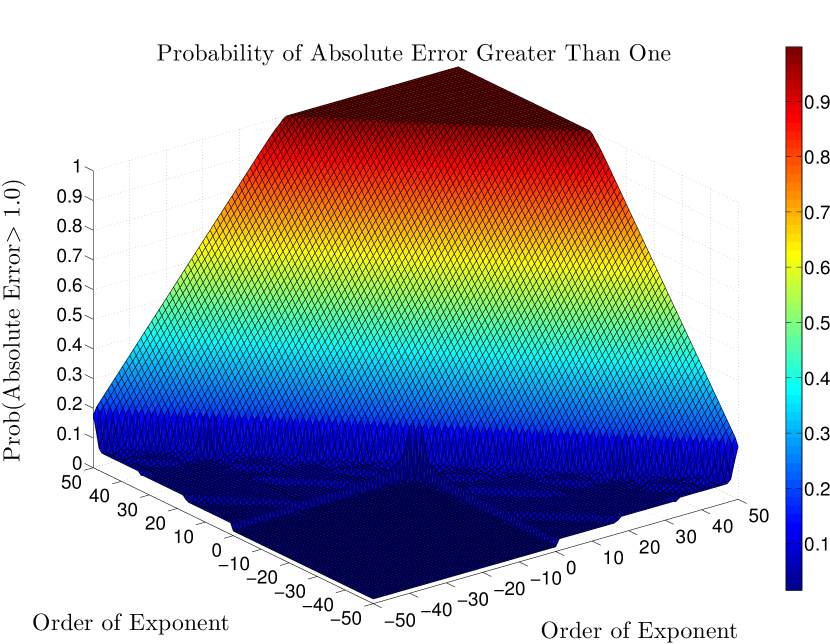
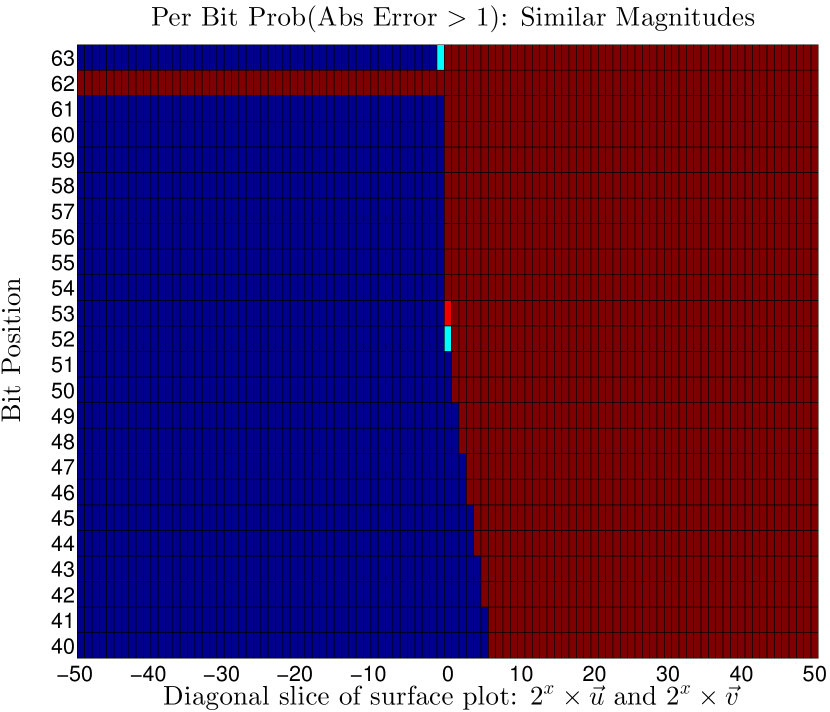
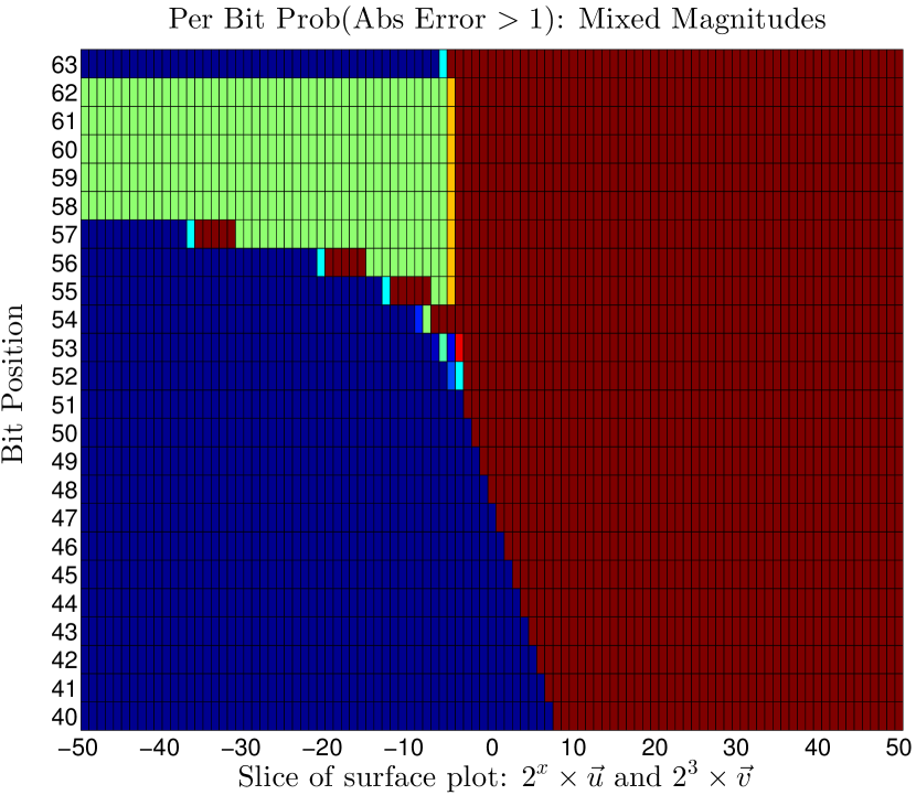
Figure 6(a) presents a surface plot as described in the Visualization bullet. To interpret this graph, the x-axis indicates the magnitude that all elements of the vector $\boldsymbol{\mathbf{u}}$ were forced to have while the mantissa was randomly generated. Likewise, the y-axis indicates the magnitude that all elements of the vector $\boldsymbol{\mathbf{v}}$ were forced to have. Each x-y intersection represents 1,000,000 random vector samples, where the dot product was computed and failures tallied. The height of the surface at an $(x,y)$ location indicates the probability of observing an absolute error larger than $1$ given a single bit flip. From this surface, one may immediately recognize the unusual structure of these graphs: When both vectors have magnitudes larger than $2^{0}$, the probability of failure is noticeably higher; yet, when both vectors have magnitudes less than or euqal to $2^{0}$, the probability of failure is approaching zero.

The key finding presented in Figure 6(a), is that when we operate on vectors that are normalized, e.g., values in the range $[0,1]$, we have a very low probability of seeing a large error should a bit flip occur. The lowest probability, i.e., the flat region in the quadrant $[0,-50]\times[0,-50]$, is precisely $\mathrm{Prob}(\mathrm{Abs~{}Error}>1)=0.015625$, which is $1/64$. The single bit that can introduce absolute error larger than one is the most significant exponent bit. Also, should the most significant exponent bit flip, the error is quite large and can be detected [15].

VI-C Per Bit Analysis of Surface Plot

To better understand the structure of the surface plot, we take two slices of the surface and look at the per-bit probability of a failure (Figures 6(b) and 6(c)). The slices chosen feature dot products of vectors with similar relative magnitudes and dot products of vectors of many magnitudes (the x-axis) with a vector that contains magnitudes up to $2^{3}$. Intuitively, these figures slice from the back-most corner of Figure 6(a) to the front for similar magnitudes (Figure 6(b)), and they slice from the left to right for Figure 6(c).

We have shown why this shape should be expected in Figure 3, and in the example presented in § V. This feature is an artifact of how the exponent is implemented in the IEEE-754 specification, i.e., a biased exponent. The lowest probability presented in the surface plot is $0.015625=1/64$, we can graphically show this in Figure 6(b), where one can see that bit #62 (2^nd from the top), is the only bit that can contribute large error. We also show that the sign and mantissa bits can not introduce large error when values are in the range $[0,1]$.

Conversely, Figure 6(c) shows that when mixing large and small values, we expect to see large errors for faults. The green shading in Figure 6(c) (upper left quadrant) indicates a roughly 50% chance that we see an absolute error larger than one. The reason for this is that values larger than 2 have a binary pattern that introduces large error most of the time (recall Figure 4).The increased likelihood of large error from the large numbers, coupled with the low chance from small numbers, creates a scenario where it is equally likely to see both large and small absolute errors. The more we deviate from operating on numbers in the range $[0,1]$, the closer we get to having a 50/50 chance of seeing a large error (see the mantissa bits slowly becoming green as well).

VI-D Comparison of the Analytic Model and Monte Carlo Sampling

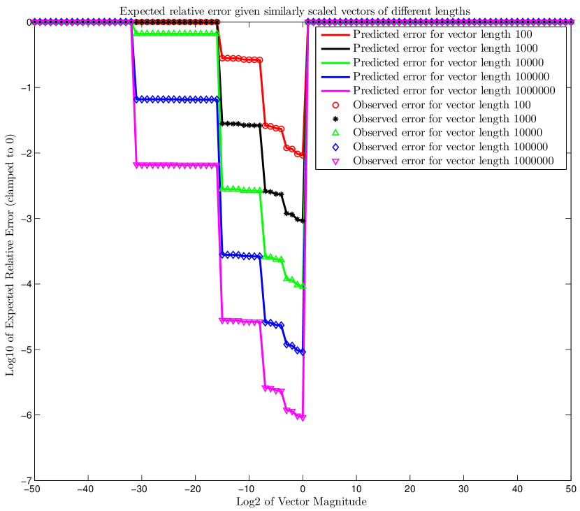
In Figure 7, we compare the error observed while performing Monte Carlo sampling with the expected error computed from our model. We sampled up to $M=$ 1 million random vectors per data point, which implies a Monte Carlo error of $error_{MC}=1/\sqrt{M}\approx 0.001$. We observe a perfect fit, which is to be expected because we have analytically shown that the exponent bits dictate the size of the absolute error we will observe. Even with random sign and mantissa bits evaluated, we see that the likelihood of experiencing a large error is entirely determined by the exponent bits.

Figure 7: Comparison of observed error caused by a flip in the exponent, excluding the most significant bit, for sampled vector sizes having similar relative magnitudes.

VII Extension to Matrices and Iterative Solvers

Having recognized that dot products on numbers less than one can produce errors less than one, we will relate this idea to matrix equilibration. We then provide an example of how to use this concept in an sparse iterative solver (GMRES), while exhaustively counting the possible errors that can be introduced.

VII-A Matrix Equilibration

The idea of scaled vectors is analogous to vector normalization, i.e., $\left\|\boldsymbol{\mathbf{u}}\right\|_{2}=1$. Applied to matrices in the context of solving linear systems, scaling takes the form of matrix equilibration: for a matrix $\boldsymbol{\mathbf{A}}$, scale the rows and columns such that $\left\|\boldsymbol{\mathbf{A}}\right\|_{\infty}=1$. Scaling can also be performed before a matrix is created, for example the equations leading to the matrix can be scaled prior to assembling a matrix. To scale a sparse matrix after its creation, we use a sparse matrix implementation of LAPACK’s equilibration routine DGEEQU [27]. Equilibration does not cause fill, i.e., it will not increase the number of non-zeros. In general, equilibrating a matrix is only beneficial, but equilibration may not be practical in all cases.

VII-B GMRES

The Generalized Minimum Residual method (GMRES) of Saad and Schultz [28] is a Krylov subspace method for solving large, sparse, possibly non-symmetric linear systems $\boldsymbol{\mathbf{A}}\boldsymbol{\mathbf{x}}=\boldsymbol{\mathbf{b}}$. GMRES is based on the Arnoldi process [29], which uses orthogonal projections and basis vectors normalized to length one. Arnoldi and GMRES relate to this work because the orthogonalization phase of Arnoldi is often Modified Gram-Schmidt or Classical Gram-Schmidt, which are dot product heavy kernels.

We present the GMRES algorithm in Algorithm 1. The Arnoldi process is expressed on Lines 8–28 in Algorithm 1. At its core is the Modified Gram-Schmidt (MGS) process, which constructs a vector orthogonal to all previous basis vectors $\boldsymbol{\mathbf{q}}_{i}$. The MGS process begins on Line 12 and completes on Line 17. We now describe how we instrument the orthogonalization phase and count the absolute errors that could be injected.

Algorithm 1 GMRES

1:Linear system $\boldsymbol{\mathbf{A}}\boldsymbol{\mathbf{x}}=\boldsymbol{\mathbf{b}}$ and initial guess $\boldsymbol{\mathbf{x}}_{0}$

2:Approximate solution $\boldsymbol{\mathbf{x}}_{m}$ for some $m\geq 0$

3:

4:$\boldsymbol{\mathbf{r}}_{0}:=\boldsymbol{\mathbf{b}}-\boldsymbol{\mathbf{A}}\boldsymbol{\mathbf{x}}_{0}$$\triangleright$ Initial residual vector

5:

6:$\beta:=\left\|\boldsymbol{\mathbf{r}}_{0}\right\|_{2}$, $\boldsymbol{\mathbf{q}}_{1}:=\boldsymbol{\mathbf{r}}_{0}/\beta$

7:

8:for $j=1,2,\dots$ until convergence do

9:

10:$\boldsymbol{\mathbf{v}}_{j+1}:=\boldsymbol{\mathbf{A}}\boldsymbol{\mathbf{q}}_{j}$$\triangleright$ Apply the matrix $A$

11:

12:for $i=1,2,\dots,j$ do$\triangleright$ Orthogonalize

13:

14:$h_{i,j}:=\boldsymbol{\mathbf{q}}_{i}\cdot\boldsymbol{\mathbf{v}}_{j+1}$

15:

16:$\boldsymbol{\mathbf{v}}_{j+1}:=\boldsymbol{\mathbf{v}}_{j+1}-h_{i,j}\boldsymbol{\mathbf{q}}_{i}$

17:end for

18:

19:$h_{j+1,j}:=\left\|\boldsymbol{\mathbf{v}}_{j+1}\right\|_{2}$

20:

21:if $h_{j+1,j}\approx 0$ then

22:

23:Solution is $\boldsymbol{\mathbf{x}}_{j-1}$$\triangleright$ Happy breakdown

24:

25:return

26:end if

27:

28:$\boldsymbol{\mathbf{q}}_{j+1}:=\boldsymbol{\mathbf{v}}_{j+1}/h_{j+1,j}$$\triangleright$ New basis vector

29:

30:$\boldsymbol{\mathbf{y}}_{j}:=\displaystyle\operatornamewithlimits{arg\,min}_{y}\left\|\boldsymbol{\mathbf{H}}({1}\nobreak\mskip 1.0mu\mathpunct{}\nonscript\mkern-3.0mu{:}\mskip 1.0mu{}{j+1},{1}\nobreak\mskip 1.0mu\mathpunct{}\nonscript\mkern-3.0mu{:}\mskip 1.0mu{}{j})\boldsymbol{\mathbf{y}}-\beta\boldsymbol{\mathbf{e}}_{1}\right\|_{2}$

31:

32:$\boldsymbol{\mathbf{x}}_{j}:=\boldsymbol{\mathbf{x}}_{0}+[\boldsymbol{\mathbf{q}}_{1},\boldsymbol{\mathbf{q}}_{2},\dots,\boldsymbol{\mathbf{q}}_{j}]\boldsymbol{\mathbf{y}}_{j}$$\triangleright$ Compute solution update

33:end for

VII-C Instrumentation and Evaluation

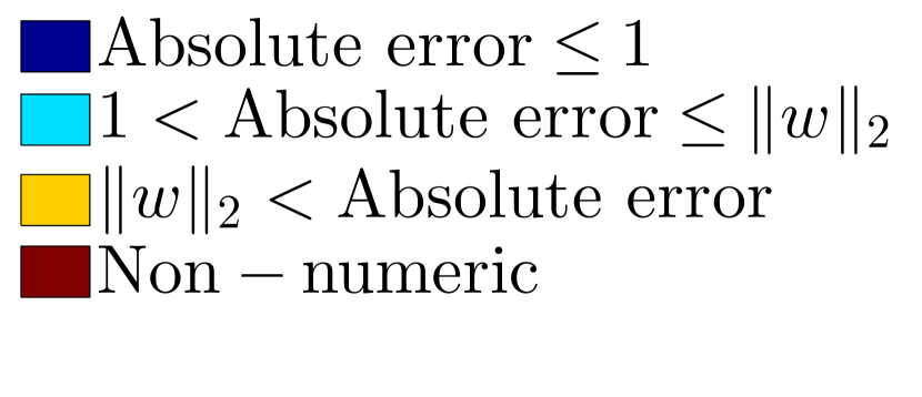
To demonstrate the benefit of data scaling we have chosen 3 test matrices. We instrument the code and for each dot product in the orthogonalization phase we determine an interval that describes the range of values possible in the vectors. Then using our fault model, we compute the absolute errors that are possible. Since we know the basis vectors ($\boldsymbol{\mathbf{q}}_{i}$) are normal, the intervals for the values in the vectors are [0,1]. We compute the min and max for the unknown vector $\boldsymbol{\mathbf{v}}$, and this determines the interval for the values in $\boldsymbol{\mathbf{v}}$. We use the intervals and our fault model to evaluate all absolute errors that can be introduced from a single bit flip in the input vectors. We classify the absolute error into four classes:

1. Absolute error less than 1.0,

2. Absolute error greater than or equal to 1.0, but less than or equal to $\left\|\boldsymbol{\mathbf{A}}\right\|_{2}$,

3. Absolute error greater $\left\|\boldsymbol{\mathbf{A}}\right\|_{2}$.

4. Error that is non-numeric, e.g., Inf or NaN.

We choose to include the 2^nd class of errors due to recent work by by Elliott et al. [15] that demonstrates how to use a norm bound on the Arnoldi process to filter out large errors in orthogonalization.

Classes 1 and 2 are undetectable, while Classes 3 and 4 are detectable. Our goal is to ensure that should a bit flip, the error falls into Classes 1, 3, and 4 while minimizing or eliminating the occurrence of Class 2 errors. We refer to Class 2 errors as the grey area, as they are undetectable errors that we consider to be large.

VII-C1 Sample Problems

We have chosen three sample matrices to demonstrate our technique. To ensure reproducibility, we did not create any of these matrices from scratch, rather we used readily available matrices. The first matrix arises from a second-order centered finite difference discretization of the Poisson equation. We generated this matrix using MATLAB’s built-in Gallery functionality. The second matrix, CoupCons3D, presents a more realistic linear system. It comes from the University of Florida Sparse Matrix Collection [30] and arises from a fully coupled poroelastic problem. The matrix is symmetric in pattern, but not symmetric in values. It is also fairly large, and has explicitly stored zero values. The matrix is poorly scaled, with a mixture of large and small values. The final matrix, mult_dcop_03, is also from the Florida Sparse Matrix Collection. It arises from a circuit simulation problem, and has good scaling inherently. We have summarized the characteristics of each matrix in Table II.

TABLE II: Sample Matrices

Properties	Poisson100	CoupCons3D	mult_dcop_03
number of rows	10,000	416,800	25,187
number of columns	10,000	416,800	25,187
nonzeros	49,600	17,277,420	193,216
structural full rank	yes	yes	yes
explicit zero entries	0	5,044,916	0
type	real	real	real
structure	symmetric	nonsymmetric	nonsymmetric
positive definite	yes	no	no

We now scale the Poisson and CoupCons3D matrices and right-hand side vectors such that they are equilibrated. Table III summarizes the norms for each of our test matrices. We use the infinity norm ($\left\|A\right\|_{\infty}\approx 1$) to measure whether a matrix is well scaled. One can see that both the Poisson and mult_dcop_03 matrices have infinity norms not too much larger than one, while the CoupCons3D matrix is inherently poorly scaled. Our equilibration code ran out of memory when attempting to equilibrate mult_dcop_03, but it is already well scaled.

TABLE III: Norms of Sample Matrices ^†

Norm	Poisson Equation		CoupCons3D
	No Scaling	Scaling	No Scaling	Scaling
$\left\|\boldsymbol{\mathbf{A}}\right\|_{\infty}$	$8.0$	$2.0$	$1.30\times 10^{6}$	$1.0$
$\left\|\boldsymbol{\mathbf{A}}\right\|_{2}$	$7.999$	$1.999$	$1.20\times 10^{6}$	$1.0$
$\left\|\boldsymbol{\mathbf{A}}\right\|_{F}$	$4.46\times 10^{2}$	$1.12\times 10^{2}$	$2.75\times 10^{6}$	$2.91\times 10^{2}$
† mult_dcop_03 has $\left\|\boldsymbol{\mathbf{A}}\right\|_{\infty}=35.5$.

VII-D Results

We ran Algorithm 1 for 1000 total iterations, using a restart value of 25. By instrumenting the code, we determined the numerical range of values each vector contained, and then computed the possible absolute error that a bit flip could introduce. We classified the absolute error according to § VII-C, and counted each class of errors for the duration of the algorithm. Figure 8 shows how these errors map to our classes of errors when the matrices are scaled versus not scaled.

(a) Poisson, no scaling.

(b) CoupCons3D, no scaling.

(c) Poisson, equilibrated

(d) CoupCons3D, equilibrated.

(e) mult_dcop_03, pre-scaled.

Figure 8: Number of possible absolute errors from dot products in Algorithm 1 in orthogonalization kernel. Class 1: $err<1.0$ (blue), Class 2: $1.0\geq err\leq\left\|\boldsymbol{\mathbf{A}}\right\|_{2}$ (light blue), Class 3: $\left\|\boldsymbol{\mathbf{A}}\right\|_{2}>err$ (yellow), and Class 4: Non-numeric (red).

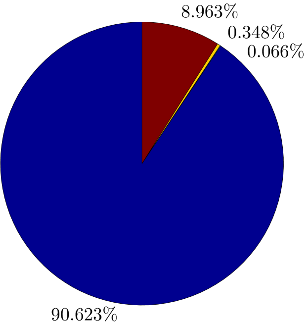
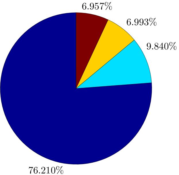
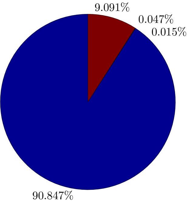
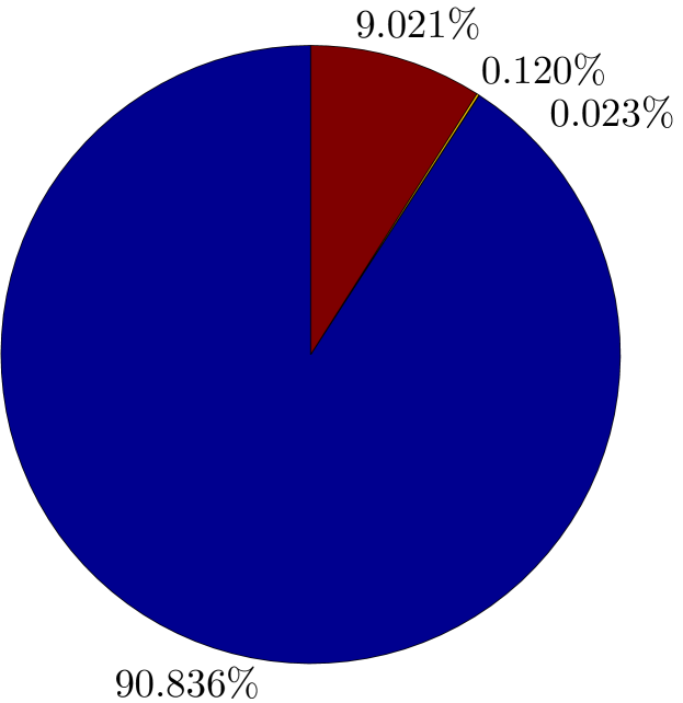
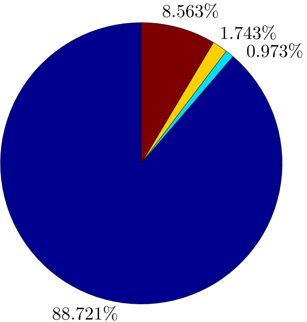
A large proportion of the absolute errors possible in orthogonalization fall into Class 1 (undetectable and small). We can explain this distribution given that the vectors $\boldsymbol{\mathbf{q}}_{i}$ are normalized (a side effect of GMRES being derived from the Arnoldi process). Given normalized vectors, we know that of all the dot products in Gram-Schmidt orthogonalization, at least one of the vectors has data in the interval $[0,1]$. We previously established that the interval $[0,1]$ aids in minimizing absolute error if a bit perturbs a dot product. Now, we show how equilibrating the input matrices can assist in forcing the non-normalized vector ($\boldsymbol{\mathbf{v}}_{j+1}$) as close as possible to being in the normalized interval.

The results show the benefits of using well-scaled matrices. Figures 8(a) and 8(e) show the Poisson problem (with no equilibration) and the mult_dcop_03 matrices, which both have good scaling (see Table III). These problems experience a higher distribution of absolute errors less than one than the poorly scaled CoupCons3D matrix (see Figure 8(b)). For the matrices that can be equilibrated, we see that scaling the input matrices is never detrimental, and will only improve fault tolerance, e.g., compare CoupCons3D before scaling in Figure 8(b) versus after scaling in Figure 8(d).

The pie charts are not probabilistic, that is, they do not convey the likelihood of observing such an error. Rather, these charts characterize the possible errors when given specific data. Consider an arbitrary length vector $\boldsymbol{\mathbf{x}}$, we can determine the range of values in the vector, e.g., $x_{i}\in[a,b]$, but we do not know how many of each value, or in what order they occur. Obtaining fine-grained statistics would involve evaluating every element of the vector, or constructing a probabilistic model that captures the distribution of values in each vector.

Since we consider the impact of a single bit flip, it is sufficient to follow the methodology presented in § V. That is, we may not know the distribution and order of numbers in the vectors, but we can model every possible error by assuming that each value in the interval could be used in an operation with every value of the other interval. This Cartesian product guarantees that we have counted all possible errors for IEEE-754 double precision numbers in an interval, including errors that may not occur because the vector does not contain that specific number, or because of the ordering.

VII-D1 Error Distribution

Our results show that scaling tends to produce a distribution of absolute error that is roughly $91\%$ less than or equal to one, while $9\%$ are non-numeric. This is expected when most of the numbers are near one. Flipping the most significant exponent bit produces $11111111111$, which will generate a non-numeric value. Similarly, the $10$ remaining exponent bits will produce error less than one — that is, $1/11\approx 9\%$ and $10/11\approx 91\%$. As previously discussed, the mantissa errors are determined entirely by the exponent bits.

VII-E Multiple Bit Flips

While this work intentionally focuses on single bit flips, the key finding that normalized data is better to operate on when performing dot products, gives some insight into how multiple bit flips in data may behave. For example, we know that a fault in the fractional component of a floating point number will produce an absolute error bound above by the order of magnitude of the original value. That is, we could flip all 52 bits of the mantissa and the error bound from our model would still be valid (e.g., Eq. (8) or Eq.(4)). In regard to exponent flips, we have shown both analytically and experimentally that when operating on normalized values, only 1 exponent bit per 64 bit value can introduce large error. Should the values all be normalized, flipping $1\to 0$ will minimize the value subject to Table I. Experiencing more than a single bit flip would only serve to “shrink” the value even more. We intentionally do not speculate about how and why multiple bit flips can occur, but we have shown that operating on normalized values skews the probability of experiencing large error.

VIII Conclusion

Our results indicate a clear benefit to good scaling. We have shown that a widely used numerical method (the Arnoldi process coupled with Gram-Schmidt orthogonalization) inherently minimizes absolute error in dot products. Furthermore, standard matrix equilibration algorithms can be used to scale input matrices, which further enhance the inherent robustness of the Arnoldi process. We demonstrated our theoretical finding experimentally by instrumenting the GMRES iterative solver, which is based on the Arnoldi process.

We cannot enforce that data are always normalized. Some linear systems may be inherently poorly scaled, or it may be impractical to equilibrate them. We can advocate that scaling, while typically used to improve numerical stability and reduce the loss of precision, can also benefit fault resilience. We have shown that this result has broad applicability, because many iterative solvers are based on orthogonal projections using normalized vectors, i.e., they create an orthonormal basis. While this work does not propose an end-to-end solution to soft errors, it does indicate that data scaling can help mitigate the impact of such errors should they occur.

References

- [1] S. Michalak, A. Dubois, C. Storlie, H. Quinn, W. Rust, D. DuBois, D. Modl, A. Manuzzato, and S. Blanchard, “Assessment of the impact of cosmic-ray-induced neutrons on hardware in the Roadrunner supercomputer,” Device and Materials Reliability, IEEE Transactions on, vol. 12, no. 2, pp. 445–454, 2012.
- [2] E. N. M. Elnozahy, R. Bianchini, T. El-Ghazawi, A. Fox, F. Godfrey, A. Hoisie, K. McKinley, R. Melhem, J. S. Plank, P. Ranganathan, and J. Simons, “System resilience at extreme scale,” Defense Advanced Research Project Agency (DARPA), Tech. Rep., 2008.
- [3] P. M. Kogge et al., “ExaScale Computing Study: Technology Challenges in Achieving Exascale Systems,” University of Notre Dame CSE Department, Tech. Rep. TR-2008-13, September 2008.
- [4] F. Cappello, G. A. A. Geist, W. D. B. Gropp, L. V. S. Kale, W. T. C. B. Kramer, and M. Snir, “Toward exascale resilience,” University of Illinois at Urbana-Champaign (UIUC) - Institut National de Recherche en Informatique et en Automatique (INRIA) Joint Laboratory on PetaScale Computing, Tech. Rep. TR-JLPC-09-01, Jun. 2009.
- [5] I. S. Haque and V. S. Pande, “Hard data on soft errors: A large-scale assessment of real-world error rates in GPGPU,” in Proceedings of the 2010 10th IEEE/ACM International Conference on Cluster, Cloud and Grid Computing, ser. CCGRID ’10. Washington, DC, USA: IEEE Computer Society, 2010, pp. 691–696.
- [6] C. C. Paige, M. Rozložník, and Z. Strakoš, “Modified Gram-Schmidt (MGS), least squares, and backward stability of MGS-GMRES,” SIAM J. Matrix Anal. Appl., vol. 28, no. 1, pp. 264–284, 2006.
- [7] V. Howle and P. Hough, “The effects of soft errors on krylov methods,” Feb. 2012.
- [8] V. Howle, P. Hough, M. Heroux, and E. Durant, “Soft errors in linear solvers as integrated components of a simulation,” Apr. 2010.
- [9] M. Shantharam, S. Srinivasmurthy, and P. Raghavan, “Characterizing the impact of soft errors on iterative methods in scientific computing,” in Proceedings of the international conference on Supercomputing, ser. ICS ’11. New York, NY, USA: ACM, 2011, pp. 152–161.
- [10] G. Bronevetsky and B. de Supinski, “Soft error vulnerability of iterative linear algebra methods,” in Proceedings of the 22nd annual international conference on Supercomputing, ser. ICS ’08. New York, NY, USA: ACM, 2008, pp. 155–164.
- [11] J. Sloan, R. Kumar, and G. Bronevetsky, “Algorithmic approaches to low overhead fault detection for sparse linear algebra,” in Proceedings of the 2012 42nd Annual IEEE/IFIP International Conference on Dependable Systems and Networks (DSN), ser. DSN ’12. Washington, DC, USA: IEEE Computer Society, 2012, pp. 1–12.
- [12] D. Li, J. Vetter, and W. Yu, “Classifying soft error vulnerabilities in extreme-scale scientific applications using a binary instrumentation tool,” in Supercomputing, Nov. 2012.
- [13] P. G. Bridges, K. B. Ferreira, M. A. Heroux, and M. Hoemmen, “Fault-tolerant linear solvers via selective reliability,” ArXiv e-prints, Jun. 2012.
- [14] P. Sao and R. Vuduc, “Self-stabilizing iterative solvers,” in Proceedings of the Workshop on Latest Advances in Scalable Algorithms for Large-Scale Systems, ser. ScalA ’13. New York, NY, USA: ACM, 2013, pp. 4:1–4:8.
- [15] J. Elliott, M. Hoemmen, and F. Mueller, “Evaluating the impact of SDC on the GMRES iterative solver,” in 28th IEEE International Parallel & Distributed Processing Symposium (IEEE IPDPS 2014), Phoenix, USA, May 2014.
- [16] D. Boley, G. H. Golub, S. Makar, N. Saxena, and E. J. Mccluskey, “Floating point fault tolerance with backward error assertions,” IEEE Transactions on Computers, vol. 44, pp. 302–311, 1995.
- [17] K.-H. Huang and J. A. Abraham, “Algorithm-based fault tolerance for matrix operations,” IEEE Transactions on Computers, vol. C-33, no. 6, pp. 518–528, Jun. 1984.
- [18] P. Du, A. Bouteiller, G. Bosilca, T. Herault, and J. Dongarra, “Algorithm-based fault tolerance for dense matrix factorizations,” SIGPLAN Not., vol. 47, no. 8, pp. 225–234, Feb. 2012.
- [19] C. J. Anfinson and F. T. Luk, “Linear algebraic model of algorithm-based fault tolerance,” IEEE Transactions on Computers, vol. 37, no. 12, pp. 1599–1604, 1988.
- [20] T. Davies, C. Karlsson, H. Liu, C. Ding, and Z. Chen, “High performance LINPACK benchmark: A fault tolerant implementation without checkpointing,” in International Conference on Supercomputing, May 2011, pp. 162–171.
- [21] Z. Chen, “Extending algorithm-based fault tolerance to tolerate fail-stop failures in high performance distributed environments,” in International Parallel and Distributed Processing Symposium, Apr. 2008.
- [22] ——, “Algorithm-based recovery for iterative methods without checkpointing,” in Symposium on High-Performance Parallel and Distributed Computing, Jun. 2011, pp. 73–84.
- [23] A. Al-Yamani, N. Oh, and E. J. McCluskey, “Performance evaluation of checksum-based ABFT,” in Symposium on Defect and Fault Tolerance in VLSI Systems (DFT 2001), Oct. 2001, pp. 461–466.
- [24] P. Banerjee, J. T. Rahmeh, C. Stunkel, V. S. Nair, K. Roy, V. Balasubramanian, and J. A. Abraham, “Algorithm-based fault tolerance on a hypercube multiprocessor,” Computers, IEEE Transactions on, vol. 39, no. 9, pp. 1132–1145, 1990.
- [25] Y. Kim, J. S. Plank, and J. J. Dongarra, “Fault tolerant matrix operations using checksum and reverse computation,” in Symposium on the Frontiers of Massively Parallel Computing, Oct. 1996, pp. 70–77.
- [26] E. J. Candès and P. Randall, “Highly robust error correction by convex programming,” IEEE Trans. Inform. Theory, vol. 54, pp. 2829–2840, 2006.
- [27] E. Anderson, Z. Bai, C. Bischof, S. Blackford, J. Demmel, J. Dongarra, J. D. Croz, A. Greenbaum, S. Hammarling, A. McKenney, and D. Sorensen, LAPACK Users’ Guide, 3rd ed. Philadelphia, PA, USA: SIAM, 1999.
- [28] Y. Saad and M. H. Schultz, “GMRES: A generalized minimal residual algorithm for solving nonsymmetric linear systems,” SIAM J. Sci. Stat. Comput., vol. 7, no. 3, pp. 856–869, Jul. 1986.
- [29] W. E. Arnoldi, “The principle of minimized iterations in the solution of the matrix eigenvalue problem,” Quarterly of Applied Mathematics, vol. 9, pp. 17–29, 1951.
- [30] T. A. Davis and Y. Hu, “The University of Florida Sparse Matrix Collection,” ACM Transactions on Mathematical Software, vol. 38, no. 1, pp. 1:1–1:25, 2011.