Scalable Object Detection using Deep Neural Networks

Abstract

Deep convolutional neural networks have recently achieved state-of-the-art performance on a number of image recognition benchmarks, including the ImageNet Large-Scale Visual Recognition Challenge (ILSVRC-2012). The winning model on the localization sub-task was a network that predicts a single bounding box and a confidence score for each object category in the image. Such a model captures the whole-image context around the objects but cannot handle multiple instances of the same object in the image without naively replicating the number of outputs for each instance. In this work, we propose a saliency-inspired neural network model for detection, which predicts a set of class-agnostic bounding boxes along with a single score for each box, corresponding to its likelihood of containing any object of interest. The model naturally handles a variable number of instances for each class and allows for cross-class generalization at the highest levels of the network. We are able to obtain competitive recognition performance on VOC2007 and ILSVRC2012, while using only the top few predicted locations in each image and a small number of neural network evaluations.

1 Introduction

Object detection is one of the fundamental tasks in computer vision. A common paradigm to address this problem is to train object detectors which operate on a subimage and apply these detectors in an exhaustive manner across all locations and scales. This paradigm was successfully used within a discriminatively trained Deformable Part Model (DPM) to achieve state-of-art results on detection tasks [6].

The exhaustive search through all possible locations and scales poses a computational challenge. This challenge becomes even harder as the number of classes grows, since most of the approaches train a separate detector per class. In order to address this issue a variety of methods were proposed, varying from detector cascades, to using segmentation to suggest a small number of object hypotheses [14, 2, 4].

In this paper, we ascribe to the latter philosphy and propose to train a detector, called “DeepMultiBox”,’ which generates a few bounding boxes as object candidates. These boxes are generated by a single DNN in a class agnostic manner. Our model has several contributions. First, we define object detection as a regression problem to the coordinates of several bounding boxes. In addition, for each predicted box the net outputs a confidence score of how likely this box contains an object. This is quite different from traditional approaches, which score features within predefined boxes, and has the advantage of expressing detection of objects in a very compact and efficient way.

The second major contribution is the loss, which trains the bounding box predictors as part of the network training. For each training example, we solve an assignment problem between the current predictions and the groundtruth boxes and update the matched box coordinates, their confidences and the underlying features through Backpropagation. In this way, we learn a deep net tailored towards our localization problem. We capitalize on the excellent representation learning abilities of DNNs, as recently exeplified recently in image classification [10] and object detection settings [13], and perform joint learning of representation and predictors.

Finally, we train our object box predictor in a class-agnostic manner. We consider this as a scalable way to enable efficient detection of large number of object classes. We show in our experiments that by only post-classifying less than ten boxes, obtained by a single network application, we can achieve state-of-art detection results. Further, we show that our box predictor generalizes over unseen classes and as such is flexible to be re-used within other detection problems.

2 Previous work

The literature on object detection is vast, and in this section we will focus on approaches exploiting class-agnostic ideas and addressing scalability.

Many of the proposed detection approaches are based on part-based models [7], which more recently have achieved impressive performance thanks to discriminative learning and carefully crafted features [6]. These methods, however, rely on exhaustive application of part templates over multiple scales and as such are expensive. Moreover, they scale linearly in the number of classes, which becomes a challenge for modern datasets such as ImageNet.

To address the former issue, Lampert et al. [11] use a branch-and-bound strategy to avoid evaluating all potential object locations. To address the latter issue, Song et al. [12] use a low-dimensional part basis, shared across all object classes. A hashing based approach for efficient part detection has shown good results as well [3].

A different line of work, closer to ours, is based on the idea that objects can be localized without having to know their class. Some of these approaches build on bottom-up classless segmentation [9]. The segments, obtained in this way, can be scored using top-down feedback [14, 2, 4]. Using the same motivation, Alexe et al. [1] use an inexpensive classifier to score object hypotheses for being an object or not and in this way reduce the number of location for the subsequent detection steps. These approaches can be thought of as Multi-layered models, with segmentation as first layer and a segment classification as a subsequent layer. Despite the fact that they encode proven perceptual principles, we will show that having deeper models which are fully learned can lead to superior results.

Finally, we capitalize on the recent advances in Deep Learning, most noticeably the work by Krizhevsky et al. [10]. We extend their bounding box regression approach for detection to the case of handling multiple objects in a scalable manner. DNN-based regression, to object masks however, has been applied by Szegedy et al. [13]. This last approach achieves state-of-art detection performance but does not scale up to multiple classes due to the cost of a single mask regression.

3 Proposed approach

We aim at achieving a class-agnostic scalable object detection by predicting a set of bounding boxes, which represent potential objects. More precisely, we use a Deep Neural Network (DNN), which outputs a fixed number of bounding boxes. In addition, it outputs a score for each box expressing the networkconfidence of this box containing an object.

Model

To formalize the above idea, we encode the $i$-th object box and its associated confidence as node values of the last net layer:

Bounding box:

we encode the upper-left and lower-right coordinates of each box as four node values, which can be written as a vector $l_{i}\in\mathbb{R}^{4}$. These coordinates are normalized w. r. t. image dimensions to achieve invariance to absolute image size. Each normalized coordinate is produced by a linear transformation of the last hidden layer.

Confidence:

the confidence score for the box containing an object is encoded as a single node value $c_{i}\in[0,1]$. This value is produced through a linear transformation of the last hidden layer followed by a sigmoid.

We can combine the bounding box locations $l_{i}$, $i\in\{1,\ldots K\}$, as one linear layer. Similarly, we can treat collection of all confidences $c_{i}$, $i\in\{1,\ldots K\}$ as the output as one sigmoid layer. Both these output layers are connected to the last hidden layers.

At inference time, out algorithm produces $K$ bounding boxes. In our experiments, we use $K=100$ and $K=200$. If desired, we can use the confidence scores and non-maximum suppression to obtain a smaller number of high-confidence boxes at inference time. These boxes are supposed to represent objects. As such, they can be classified with a subsequent classifier to achieve object detection. Since the number of boxes is very small, we can afford powerful classifiers. In our experiments, we use another DNN for classification [10].

Training Objective

We train a DNN to predict bounding boxes and their confidence scores for each training image such that the highest scoring boxes match well the ground truth object boxes for the image. Suppose that for a particular training example, $M$ objects were labeled by bounding boxes $g_{j}$, $j\in\{1,\ldots,M\}$. In practice, the number of predictions $K$ is much larger than the number of groundtruth boxes $M$. Therefore, we try to optimize only the subset of predicted boxes which match best the ground truth ones. We optimize their locations to improve their match and maximize their confidences. At the same time we minimize the confidences of the remaining predictions, which are deemed not to localize the true objects well.

To achieve the above, we formulate an assignment problem for each training example. We $x_{ij}\in\{0,1\}$ denote the assignment: $x_{ij}=1$ iff the $i$-th prediction is assigned to $j$-th true object. The objective of this assignment can be expressed as:

$$F_{\text{match}}(x,l)=\frac{1}{2}\sum_{i,j}x_{ij}||l_{i}-g_{j}||_{2}^{2}$$ (1)

where we use $L_{2}$ distance between the normalized bounding box coordinates to quantify the dissimilarity between bounding boxes.

Additionally, we want to optimize the confidences of the boxes according to the assignment $x$. Maximizing the confidences of assigned predictions can be expressed as:

$$F_{\text{conf}}(x,c)=-\sum_{i,j}x_{ij}\log(c_{i})-\sum_{i}(1-\sum_{j}x_{ij})\log(1-c_{i})$$ (2)

In the above objective $\sum_{j}x_{ij}=1$ iff prediction $i$ has been matched to a groundtruth. In that case $c_{i}$ is being maximized, while in the opposite case it is being minimized. A different interpretation of the above term is achieved if we $\sum_{j}x_{ij}$ view as a probability of prediction $i$ containing an object of interest. Then, the above loss is the negative of the entropy and thus corresponds to a max entropy loss.

The final loss objective combines the matching and confidence losses:

$$F(x,l,c)=\alpha F_{\text{match}}(x,l)+F_{\text{conf}}(x,c)$$ (3)

subject to constraints in Eq. 1. $\alpha$ balances the contribution of the different loss terms.

Optimization

For each training example, we solve for an optimal assignment $x^{*}$ of predictions to true boxes by

$$x^{*} = \arg\min_{x}F(x,l,c)$$ (4)

subject to $$x_{ij}\in\{0,1\},\sum_{i}x_{ij}=1,$$ (5)

where the constraints enforce an assignment solution. This is a variant of bipartite matching, which is polynomial in complexity. In our application the matching is very inexpensive – the number of labeled objects per image is less than a dozen and in most cases only very few objects are labeled.

Then, we optimize the network parameters via back-propagation. For example, the first derivatives of the back-propagation algorithm are computed w. r. t.  $l$ and $c$:

$$\frac{\partial F}{\partial l_{i}} = \sum_{j}(l_{i}-g_{j})x_{ij}^{*}$$ (6)

$$\frac{\partial F}{\partial c_{i}} = \frac{\sum_{j}x_{ij}^{*}c_{i}}{c_{i}(1-c_{i})}$$ (7)

Training Details

While the loss as defined above is in principle sufficient, three modifications make it possible to reach better accuracy significantly faster. The first such modification is to perform clustering of ground truth locations and find $K$ such clusters/centroids that we can use as priors for each of the predicted locations. Thus, the learning algorithm is encouraged to learn a residual to a prior, for each of the predicted locations.

A second modification pertains to using these priors in the matching process: instead of matching the $N$ ground truth locations with the $K$ predictions, we find the best match between the $K$ priors and the ground truth. Once the matching is done, the target confidences are computed as before. Moreover, the location prediction loss is also unchanged: for any matched pair of (target, prediction) locations, the loss is defined by the difference between the groundtruth and the coordinates that correspond to the matched prior. We call the usage of priors for matching prior matching and hypothesize that it enforces diversification among the predictions.

It should be noted, that although we defined our method in a class-agnostic way, we can apply it to predicting object boxes for a particular class. To do this, we simply need to train our models on bounding boxes for that class.

Further, we can predict $K$ boxes per class. Unfortunately, this model will have number of parameters growing linearly with the number of classes. Also, in a typical setting, where the number of objects for a given class is relatively small, most of these parameters will see very few training examples with a corresponding gradient contribution. We argue thusly that our two-step process – first localize, then recognize – is a superior alternative in that it allows leveraging data from multiple object types in the same image using a small number of parameters.

4 Experimental results

4.1 Network Architecture and Experiment Details

The network architecture for the localization and classification models that we use is the same as the one used by [10]. We use Adagrad for controlling the learning rate decay, mini-batches of size 128, and parallel distributed training with multiple identical replicas of the network, which achieves faster convergence. As mentioned previously, we use priors in the localization loss – these are computed using $k$-means on the training set. We also use an $\alpha$ of $0.3$ to balance the localization and confidence losses.

The localizer might output coordinates outside the crop area used for the inference. The coordinates are mapped and truncated to the final image area, at the end. Boxes are additionally pruned using non-maximum-suppression with a Jaccard similarity threshold of $0.5$. Our second model then classifies each bounding box as objects of interest or “background”.

To train our localizer networks, we generated approximately $30$ million images from the training set, applying the following procedure to each image in the training set. The samples are shuffled at the end. To train our localizer networks, we generated approximately $30$ million images from the training set by applying the following procedure to each image in the training set. For each image, we generate the same number of square samples such that the total number of samples is about ten million. For each image, the samples are bucketed such that for each of the ratios in the ranges of $0-5\%,5-15\%,15-50\%,50-100\%$, there is an equal number of samples in which the ratio covered by the bounding boxes is in the given range.

The selection of the training set and most of our hyper-parameters were based on past experiences with non-public data sets. For the experiments below we have not explored any non-standard data generation or regularization options.

In all experiments, all hyper-parameters were selected by evaluating on a held out portion of the training set (10% random choice of examples).

4.2 VOC 2007

The Pascal Visual Object Classes (VOC) Challenge [5] is the most commong benchmark for object detection algorithms. It consists mainly of complex scene images in which bounding boxes of 20 diverse object classes were labelled.

In our evaluation we focus on the 2007 edition of VOC, for which a test set was released. We present results by training on VOC 2012, which contains approx. 11000 images. We trained a $100$ box localizer as well as a deep net based classifier [10].

4.2.1 Training methodology

We trained the classifier on a data set comprising of

• $10$ million crops overlapping some object with at least $0.5$ Jaccard overlap similarity. The crops are labeled with one of the 20 VOC object classes.

• $20$ million negative crops that have at most $0.2$ Jaccard similarity with any of the object boxes. These crops are labeled with the special “background” class label.

The architecture and the selection of hyperparameters followed that of [10].

4.2.2 Evaluation methodology

In the first round, the localizer model is applied to the maximum center square crop in the image. The crop is resized to the network input size which is $220\times 220$. A single pass through this network gives us up to hundred candidate boxes. After a non-maximum-suppression with overlap threshold $0.5$, the top $10$ highest scoring detections are kept and were classified by the 21-way classifier model in a separate passes through the network. The final detection score is the product of the localizer score for the given box multiplied by the score of the classifier evaluated on the maximum square region around the crop. These scores are passed to the evaluation and were used for computing the precision recall curves.

4.3 Discussion

First, we analyze the performance of our localizer in isolation. We present the number of detected objects, as defined by the Pascal detection criterion, against the number of produced bounding boxes. In Fig. 1 plot we show results obtained by training on VOC2012. In addition, we present results by using the max-center square crop of the image as input as well as by using two scales: the max-center crop by a second scale where we select $3\times 3$ windows of size $60\%$ of the image size.

As we can see, when using a budget of $10$ bounding boxes we can localize $45.3\%$ of the objects with the first model, and $48\%$ with the second model. This shows better perfomance than other reported results, such as the objectness algorithm achieving $42\%$ [1]. Further, this plot shows the importance of looking at the image at several resolutions. Although our algorithm manages to get large number of objects by using the max-center crop, we obtain an additional boost when using higher resolution image crops.

class	aero	bicycle	bird	boat	bottle	bus	car	cat	chair	cow
DeepMultiBox	.413	.277	.305	.176	.032	.454	.362	.535	.069	.256
3-layer model [15]	.294	.558	.094	.143	.286	.440	.513	.213	.200	.193
Felz. et al. [6]	.328	.568	.025	.168	.285	.397	.516	.213	.179	.185
Girshick et al. [8]	.324	.577	.107	.157	.253	.513	.542	.179	.210	.240
Szegedy et al. [13]	.292	.352	.194	.167	.037	.532	.502	.272	.102	.348
class	table	dog	horse	m-bike	person	plant	sheep	sofa	train	tv
DeepMultiBox	.273	.464	.312	.297	.375	.074	.298	.211	.436	.225
3-layer model [15]	.252	.125	.504	.384	.366	.151	.197	.251	.368	.393
Felz. et al. [6]	.259	.088	.492	.412	.368	.146	.162	.244	.392	.391
Girshick et al. [8]	.257	.116	.556	.475	.435	.145	.226	.342	.442	.413
Szegedy et al .[13]	.302	.282	.466	.417	.262	.103	.328	.268	.398	.47

Table 1: Average Precision on VOC 2007 test of our method, called DeepMultiBox, and other competitive methods. DeepMultibox was trained on VOC2012 training data, while the rest of the models were trained on VOC2007 data.

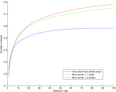
Figure 1: Detection rate of class “object” vs number of bounding boxes per image. The model, used for these results, was trained on VOC 2012.

Further, we classify the produced bounding boxes by a 21-way classifier, as described above. The average precisions (APs) on VOC 2007 are presented in Table 1. The achieved mean AP is $0.29$, which is on par with state-of-art. Note that, our running time complexity is very low – we simply use the top $10$ boxes.

Example detections and full precision recall curves are shown in Fig. 2 and Fig. 3 respectively. It is important to note that the visualized detections were obtained by using only the max-centered square image crop, i. e. the full image was used. Nevertheless, we manage to obtain relatively small objects, such as the boats in row 2 and column 2, as well as the sheep in row 3 and column 3.

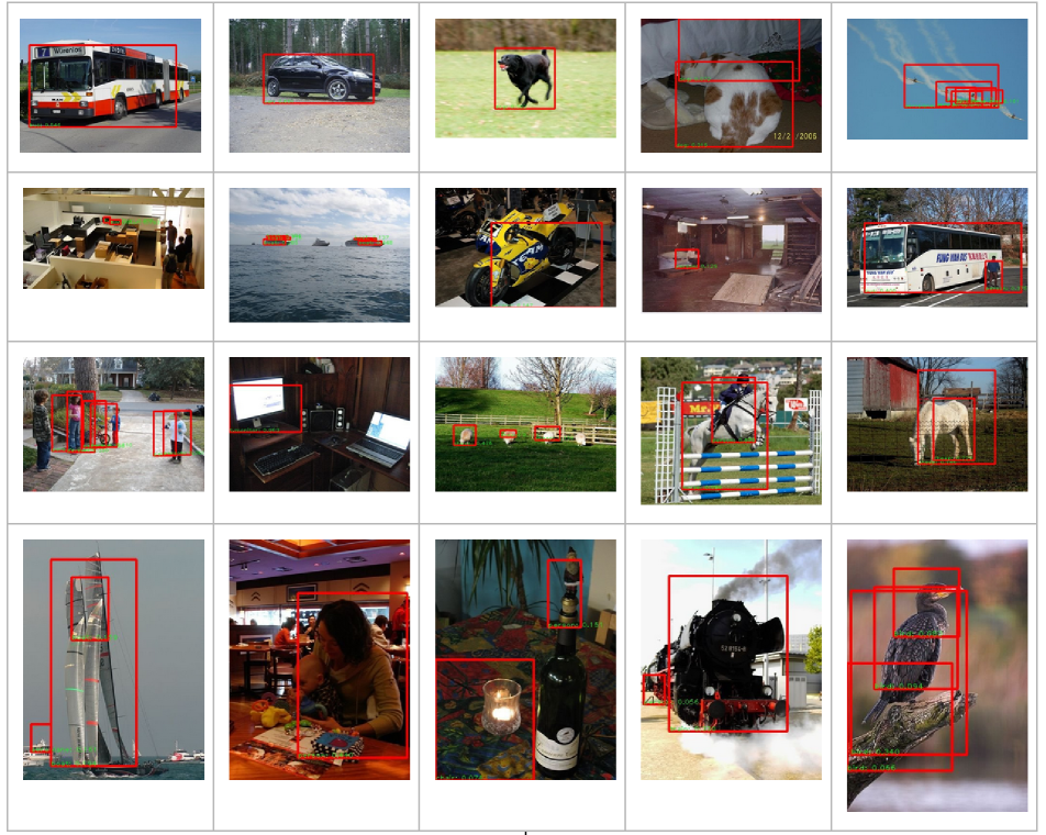
Figure 2: Sample of detection results on VOC 2007.

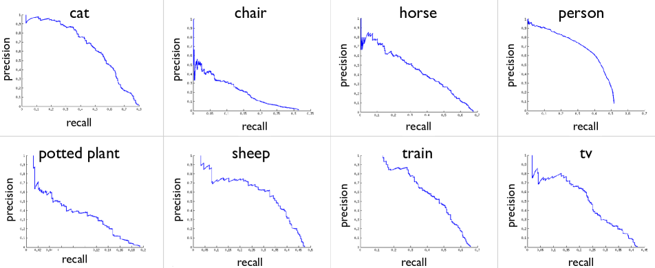
Figure 3: Precision-recall curves on selected VOC classes.

4.4 ILSVRC 2012 Detection Challenge

For this set of experiments, we used the ILSVRC 2012 detection challenge dataset. This dataset consists of 544,545 training images labeled with categories and locations of 1,000 object categories, relatively uniformly distributed among the classes. The validation set, on which the performance metrics are calculated, consists of 48,238 images.

4.4.1 Training methodology

In addition to a localization model that is identical (up to the dataset on which it is trained on) to the VOC model, we also train a model on the ImageNet Classification challenge data, which will serve as the recognition model. This model is trained in a procedure that is substantially similar to that of [10] and is able to achieve the same results on the classification challenge validation set; note that we only train a single model, instead of $7$ – the latter brings substantial benefits in terms of classification accuracy, but is $7\times$ more expensive, which is not a negligible factor.

Inference is done as with the VOC setup: the number of predicted locations is $K=100$, which are then reduced by Non-Max-Suppression (Jaccard overlap criterion of $0.4$) and which are post-scored by the classifier: the score is the product of the localizer confidence for the given box multiplied by the score of the classifier evaluated on the minimum square region around the crop. The final scores (detection score times classification score) are then sorted in descending order and only the top scoring score/location pair is kept for a given class (as per the challenge evaluation criterion).

In all experiments, the hyper-parameters were selected by evaluating on a held out portion of the training set (10% random choice of examples).

4.4.2 Evaluation methodology

The official metric of the “Classification with localization“ ILSVRC-2012 challenge is detection@5, where an algorithm is only allowed to produce one box per each of the 5 labels (in other words, a model is neither penalized nor rewarded for producing valid multiple detections of the same class), where the detection criterion is 0.5 Jaccard overlap with any of the ground-truth boxes (in addition to the matching class label).

Table 2 contains a comparison of the proposed method, dubbed DeepMultiBox, with classifying the ground-truth boxes directly and with the approach of inferring one box per class directly. The metrics reported are detection5 and classification5, the official metrics for the ILSVRC-2012 challenge metrics. In the table, we vary the number of windows at which we apply the classifier (this number represents the top windows chosen after non-max-suppression, the ranking coming from the confidence scores). The one-box-per-class approach is a careful re-implementation of the winning entry of ILSVRC-2012 (the “classification with localization” challenge), with 1 network trained (instead of 7).

Table 2: Performance of Multibox (the proposed method) vs. classifying ground-truth boxes directly and predicting one box per class

Method	det@5	class@5
One-box-per-class	61.00%	79.40%
Classify GT directly	82.81%	82.81%
DeepMultiBox, top 1 window	56.65%	73.03%
DeepMultiBox, top 3 windows	58.71%	77.56%
DeepMultiBox, top 5 windows	58.94%	78.41%
DeepMultiBox, top 10 windows	59.06%	78.70%
DeepMultiBox, top 25 windows	59.04%	78.76%

Figure 4: Some selected detection results on the ILSVRC-2012 detection challenge validation set.

We can see that the DeepMultiBox approach is quite competitive: with 5-10 windows, it is able to perform about as well as the competing approach. While the one-box-per-class approach may come off as more appealing in this particular case in terms of the raw performance, it suffers from a number of drawbacks: first, its output scales linearly with the number of classes, for which there needs to be training data. The multibox approach can in principle use transfer learning to detect certain types of objects on which it has never been specifically trained on, but which share similarities with objects that it has seen. Figure 5 explores this hypothesis by observing what happens when one takes a localization model trained on ImageNet and applies it on the VOC test set, and vice-versa. The figure shows a precision-recall curve: in this case, we perform a class-agnostic detection: a true positive occurs if two windows (prediction and groundtruth) overlap by more than 0.5, independently of their class. Interestingly, the ImageNet-trained model is able to capture more VOC windows than vice-versa: we hypothesize that this is due to the ImageNet class set being much richer than the VOC class set.

Secondly, the one-box-per-class approach does not generalize naturally to multiple instances of objects of the same type (except via the the method presented in this work, for instance). Figure 5 shows this too, in the comparison between DeepMultiBox and the one-per-class approach. Generalizing to such a scenario is necessary for actual image understanding by algorithms, thus such limitations need to be overcome, and our method is a scalable way of doing so. Evidence supporting this statement is shown in Figure 5 shows that the proposed method is able to generally capture more objects more accurately that a single-box method.

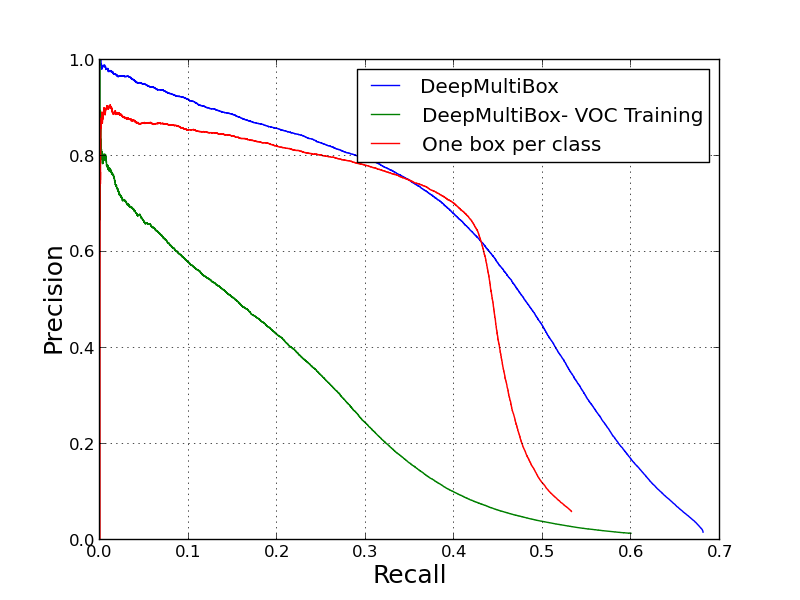
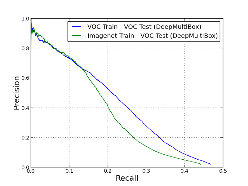
Figure 5: Class-agnostic detection on ILSVRC-2012 (left) and VOC 2007 (right).

5 Discussion and Conclusion

In this work, we propose a novel method for localizing objects in an image, which predicts multiple bounding boxes at a time. The method uses a deep convolutional neural network as a base feature extraction and learning model. It formulates a multiple box localization cost that is able to take advantage of variable number of groundtruth locations of interest in a given image and learn to predict such locations in unseen images.

We present results on two challenging benchmarks, VOC2007 and ILSVRC-2012, on which the proposed method is competitive. Moreover, the method is able to perform well by predicting only very few locations to be probed by a subsequent classifier. Our results show that the DeepMultiBox approach is scalable and can even generalize across the two datasets, in terms of being able to predict locations of interest, even for categories on which it was not trained on. Additionally, it is able to capture multiple instances of objects of the same class, which is an important feature of algorithms that aim for better image understanding.

In the future, we hope to be able to fold the localization and recognition paths into a single network, such that we would be able to extract both location and class label information in a one-shot feed-forward pass through the network. Even in its current state, the two-pass procedure (localization network followed by categorization network) entails 5-10 network evaluations, each at roughly 1 CPU-sec (modern machine). Importantly, this number does not scale linearly with the number of classes to be recognized, which makes the proposed approach very competitive with DPM-like approaches.

References

- [1] B. Alexe, T. Deselaers, and V. Ferrari. What is an object? In CVPR. IEEE, 2010.
- [2] J. Carreira and C. Sminchisescu. Constrained parametric min-cuts for automatic object segmentation. In CVPR, 2010.
- [3] T. Dean, M. A. Ruzon, M. Segal, J. Shlens, S. Vijayanarasimhan, and J. Yagnik. Fast, accurate detection of 100,000 object classes on a single machine. In CVPR, 2013.
- [4] I. Endres and D. Hoiem. Category independent object proposals. In ECCV. 2010.
- [5] M. Everingham, L. Van Gool, C. K. Williams, J. Winn, and A. Zisserman. The pascal visual object classes (voc) challenge. International journal of computer vision, 88(2):303–338, 2010.
- [6] P. F. Felzenszwalb, R. B. Girshick, D. McAllester, and D. Ramanan. Object detection with discriminatively trained part-based models. Pattern Analysis and Machine Intelligence, IEEE Transactions on, 32(9):1627–1645, 2010.
- [7] M. A. Fischler and R. A. Elschlager. The representation and matching of pictorial structures. Computers, IEEE Transactions on, 100(1):67–92, 1973.
- [8] R. B. Girshick, P. F. Felzenszwalb, and D. McAllester. Discriminatively trained deformable part models, release 5. http://people.cs.uchicago.edu/ rbg/latent-release5/.
- [9] C. Gu, J. J. Lim, P. Arbeláez, and J. Malik. Recognition using regions. In CVPR, 2009.
- [10] A. Krizhevsky, I. Sutskever, and G. Hinton. Imagenet classification with deep convolutional neural networks. In Advances in Neural Information Processing Systems 25, pages 1106–1114, 2012.
- [11] C. H. Lampert, M. B. Blaschko, and T. Hofmann. Beyond sliding windows: Object localization by efficient subwindow search. In CVPR, 2008.
- [12] H. O. Song, S. Zickler, T. Althoff, R. Girshick, M. Fritz, C. Geyer, P. Felzenszwalb, and T. Darrell. Sparselet models for efficient multiclass object detection. In ECCV. 2012.
- [13] C. Szegedy, A. Toshev, and D. Erhan. Deep neural networks for object detection. In Advances in Neural Information Processing Systems (NIPS), 2013.
- [14] K. E. van de Sande, J. R. Uijlings, T. Gevers, and A. W. Smeulders. Segmentation as selective search for object recognition. In ICCV, 2011.
- [15] L. Zhu, Y. Chen, A. Yuille, and W. Freeman. Latent hierarchical structural learning for object detection. In Computer Vision and Pattern Recognition (CVPR), 2010 IEEE Conference on, pages 1062–1069. IEEE, 2010.