bartMachine: Machine Learning with Bayesian Additive Regression Trees

Adam Kapelner, Justin Bleich bartMachine: Machine Learning with Bayesian Additive Regression Trees bartMachine: Machine Learning with Bayesian Additive Regression Trees We present a new package in R implementing Bayesian additive regression trees (BART). The package introduces many new features for data analysis using BART such as variable selection, interaction detection, model diagnostic plots, incorporation of missing data and the ability to save trees for future prediction. It is significantly faster than the current R implementation, parallelized, and capable of handling both large sample sizes and high-dimensional data. Bayesian, machine learning, statistical learning, non-parametric, R, Java Bayesian, machine learning, statistical learning, non-parametric, R, Java, Adam Kapelner
Department of Mathematics
Queens College, City University of New York
64-19 Kissena Blvd Room 325
Flushing, NY, 11367
E-mail:
URL: http://scholar.google.com/citations?user=TzgMmnoAAAAJ

1 Introduction

Ensemble-of-trees methods have become popular choices for forecasting in both regression and classification problems. Algorithms such as random forests (Breiman2001) and stochastic gradient boosting (Friedman2002) are two well-established and widely employed procedures. Recent advances in ensemble methods include dynamic trees (Taddy2011) and Bayesian additive regression trees (BART, Chipman2010), which depart from predecessors in that they rely on an underlying Bayesian probability model rather than a pure algorithm. BART has demonstrated substantial promise in a wide variety of simulations and real world applications such as predicting avalanches on mountain roads (Blattenberger2014), predicting how transcription factors interact with DNA (Zhou2008) and predicting movie box office revenues (Eliashberg2010). This paper introduces bartMachine, a new R (Rlang) package available from the Comprehensive R Archive Network at http://CRAN.R-project.org/package=bartMachine that significantly expands the capabilities of using BART for data analysis.

Currently, there exists one other implementation of BART on CRAN: BayesTree (BayesTree), the package developed by the algorithm’s original authors. One of the major drawbacks of this implementation is its lack of a predict function. Test data must be provided as an argument during the training phase of the model. Hence it is impossible to generate forecasts on future data without re-fitting withe entire model. Since the run time is not trivial, forecasting becomes an arduous exercise. A significantly faster implementation of BART that contains master-slave parallelization exists as Pratola2013, but this is only available as standalone C++ source code and not integrated with R. Additionally, a recent package dbarts allows updating of BART with new predictors and response values to incorporate BART into a larger Bayesian model. dbarts relies on BayesTree as it’s BART engine.

The goal of bartMachine is to provide a fast, easy-to-use, visualization-rich machine learning package for R users. Our implementation of BART is in Java and is integrated into R via rJava (rJava). From a runtime perspective, our algorithm is significantly faster and is parallelized, allowing computation on as many cores as desired. Not only is the model construction itself parallelized, but the additional features such as prediction, variable selection, and many others can be divided across cores as well.

Additionally, we include a variety of expanded and new features. We implement the ability to save trees in memory and provide convenience functions for prediction on test data. We also include plotting functions for both credible and predictive intervals and plots for visually inspecting convergence of BART’s Gibbs sampler. We expand variable importance exploration to include permutation tests and interaction detection. We implement recently developed features for BART including a principled approach to variable selection and the ability to incorporate in prior information for covariates (Bleich2014). We also implement the strategy found in Kapelner2013 to incorporate missing data during training and handle missingness during prediction. Table 1 emphasizes the differences in features between bartMachine and BayesTree, the two existing R implementations of BART.

Feature	bartMachine	BayesTree
Implementation Language	Java	C++
External Predict Function	Yes	No
Model Persistance Across Sessions	Yes	No
Parallelization	Yes	No
Native Missing Data Mechanism	Yes	No
Built-in Cross-Validation	Yes	No
Variable Importance	Statistical Tests	Exploratory
Tree Proposal Types	3 Types	4 Types
Partial Dependence Plots	Yes	Yes
Convergence Plots	Assess trees and $\sigma^{2}$	Assess $\sigma^{2}$
Model Diagnostics	Yes	No
Incorporation into Larger Model	No	Through dbarts

Table 1: Comparison of features between bartMachine and BayesTree.

In Section 2, we provide an overview of BART with a special emphasis on the features that have been extended. In Section 3 we provide a general introduction to the package, highlighting the novel features. Section 4 provides step-by-step examples of the regression capabilities and Section LABEL:sec:classification_features introduces additional step-by-step examples of features unique to classification problems. We conclude in Section LABEL:sec:discussion. Appendix LABEL:app:implementation discusses the details of our algorithm implementation and how it differs from BayesTree. Appendix LABEL:app:bakeoff offers predictive performance comparisons.

2 Overview of BART

BART is a Bayesian approach to nonparametric function estimation using regression trees. Regression trees rely on recursive binary partitioning of predictor space into a set of hyperrectangles in order to approximate some unknown function $f$. Predictor space has dimension of the number of variables, which we denote $p$. Tree-based regression models have an ability to flexibly fit interactions and nonlinearities. Models composed of sums of regression trees have an even greater ability than single trees to capture interactions and non-linearities as well as additive effects in $f$.

BART can be considered a sum-of-trees ensemble, with a novel estimation approach relying on a fully Bayesian probability model. Specifically, the BART model can be expressed as:

$$\boldsymbol{Y}=f(\boldsymbol{X})+\boldsymbol{\mathcal{E}}\approx\mathcal{T}_{1}^{\mathcal{M}}(\boldsymbol{X})+\mathcal{T}_{2}^{\mathcal{M}}(\boldsymbol{X})+\ldots+\mathcal{T}_{m}^{\mathcal{M}}(\boldsymbol{X})+\boldsymbol{\mathcal{E}},\quad\quad\boldsymbol{\mathcal{E}}\sim\mathcal{N}_{n}\left(\boldsymbol{0},\,\sigma^{2}\boldsymbol{I}_{n}\right)$$ (1)

where $\boldsymbol{Y}$ is the $n\times 1$ vector of responses, $\boldsymbol{X}$ is the $n\times p$ design matrix (the predictors column-joined), $\boldsymbol{\mathcal{E}}$ is the $n\times 1$ vector of noise. Here we have $m$ distinct regression trees, each composed of a tree structure, denoted by $\mathcal{T}$, and the parameters at the terminal nodes (also called leaves), denoted by $\mathcal{M}$. The two together, denoted as $\mathcal{T}^{\mathcal{M}}$ represents an entire tree with both its structure and set of leaf parameters.

The structure of a given tree $\mathcal{T}_{t}$ includes information on how any observation recurses down the tree. For each nonterminal (internal) node of the tree, there is a “splitting rule” taking the form $\boldsymbol{x}_{j}<c$ consisting of the “splitting variable” $\boldsymbol{x}_{j}$ and the “splitting value” $c$. An observation moves to the left child node if the condition set by the splitting rule is satisfied and to the right child node otherwise. The process continues until a terminal node is reached. Then, the observation receives the leaf value of the terminal node. The sum of the $m$ leaf values becomes its predicted value. We denote the set of tree’s leaf parameters as $\mathcal{M}_{t}=\{\mu_{t,1},\mu_{t,2},\ldots,\mu_{t_{b_{t}}}\}$ where $b_{t}$ is the number of terminal nodes for a given tree.

BART can be distinguished from other ensemble-of-trees models due to its underlying probability model. As a Bayesian model, BART consists of a set of priors for the structure and the leaf parameters and a likelihood for data in the terminal nodes. The aim of the priors is to provide regularization, preventing any single regression tree from dominating the total fit.

We provide an overview of the BART priors and likelihood and then discuss how draws from the posterior distribution are made. A more complete exposition can be found in Chipman2010.

2.1 Priors and likelihood

The prior for the BART model has three components (1) the tree structure itself (2) the leaf parameters given the tree structure and (3) the error variance $\sigma^{2}$ which is independent of the tree structure and leaf parameters:

$$\mathbb{P}\left(\mathcal{T}_{1}^{\mathcal{M}},\ldots,\mathcal{T}_{m}^{\mathcal{M}},\sigma^{2}\right) = \left[\prod_{t}\mathbb{P}\left(\mathcal{T}_{t}^{\mathcal{M}}\right)\right]\mathbb{P}\left(\sigma^{2}\right)=\left[\prod_{t}\mathbb{P}\left(\mathcal{M}_{t}~{}|~{}\mathcal{T}_{t}\right)\mathbb{P}\left(\mathcal{T}_{t}\right)\right]\mathbb{P}\left(\sigma^{2}\right)$$

$$= \left[\prod_{t}\prod_{\ell}\mathbb{P}\left(\mu_{t,\ell}~{}|~{}\mathcal{T}_{t}\right)\mathbb{P}\left(\mathcal{T}_{t}\right)\right]\mathbb{P}\left(\sigma^{2}\right)$$

where the last line follows from an additional assumption of conditional independence of the leaf parameters given the tree’s structure.

We first describe $\mathbb{P}\left(\mathcal{T}_{t}\right)$, the component of the prior which affects the locations of nodes within the tree. Nodes at depth $d$ are nonterminal with probability $\alpha(1+d)^{-\beta}$ where $\alpha\in(0,1)$ and $\beta\in[0,\infty]$. Depth is defined as distance from the root. Thus, the root itself has depth 0, its first child node has depth 1, etc. This prior form has the ability to enforce shallow tree structures, thereby limiting complexity of any single tree. Default values for these hyperparameters of $\alpha=0.95$ and $\beta=2$ are recommended by Chipman2010.

For nonterminal nodes, splitting rules occur in two parts. First, the predictor is randomly selected to serve as the splitting variable. In the original formulation, each available predictor is equally likely to be chosen from a discrete uniform distribution with probability that each varible selected is $1/p$. This is relaxed in our implementation to allow for a generalized Bernoulli distribution where the user specifies $p_{1},p_{2},\ldots,p_{p}$ (such that $\sum_{j=1}^{p}p_{j}=1$), where each is a probability of variable selection. See “covariate priors” (Section LABEL:subsec:cov_prior) for further details. Note that “structural zeroes,” variables that do not have any valid split values, are assigned probability zero (see Appendix LABEL:subapp:grow_step for details). Once the splitting variable is chosen, the splitting value is chosen from the multiset (the non-unique set) of available values at the node via the discrete uniform distribution.

We now describe the prior component $\mathbb{P}\left(\mathcal{M}_{t}~{}|~{}\mathcal{T}_{t}\right)$ which controls the leaf parameters. Given a tree with a set of terminal nodes, each terminal node (or leaf) has a continuous parameter (the leaf parameter) representing the “best guess” of the response in this partition of predictor space. This parameter is the fitted value assigned to any observation that lands in that node. The prior on each of the leaf parameters is given as: $\mu_{\ell}~{}{\buildrel iid\over{\sim}}~{}\mathcal{N}\left(\mu_{\mu}/m,\,\sigma^{2}_{\mu}\right)$. The expectation, $\mu_{\mu}$, is picked to be the range center, $(y_{\text{min}}+y_{\text{max}})/2$. The range center can be affected by outliers. If this is a concern, the user can log-transform the response or windsorize the response.

The variance is empirically chosen so that the range center plus or minus $k=2$ variances cover 95% of the provided response values in the training set (where $k=2$ corresponding to 95% coverage is only by default and can be customized). Thus, since there are $m$ trees, we are then automatically employing $\sigma_{\mu}$ such that $m\mu_{\mu}-k\sqrt{m}\sigma_{\mu}=y_{\text{min}}$ and $m\mu_{\mu}+k\sqrt{m}\sigma_{\mu}=y_{\text{max}}$. The aim of this prior is to provide model regularization by shrinking the leaf parameters towards the center of the distribution of the response.

The final prior is on the error variance and is chosen to be $\sigma^{2}\sim\text{InvGamma}\left(\nu/2,\,\nu\lambda/2\right)$. $\lambda$ is determined from the data so that there is a $q=90\%$ a priori chance (by default) that the BART model will improve upon the RMSE from an ordinary least squares regression. Therefore, the majority of the prior probability mass lies below the RMSE from least squares regression. Additionally, this prior limits the probability mass placed on small values of $\sigma^{2}$ to prevent overfitting.

Note that the adjustable hyperparameters are $\alpha$, $\beta$, $k$, $\nu$ and $q$. Default values generally provide good performance, but optimal tuning can be achieved via cross-validation, an automatic feature implemented and described in Section 4.2.

Along with a set of priors, BART specifies the likelihood of responses in the terminal nodes. They are assumed a priori Normal with the mean being the “best guess” in the leaf at the current moment (in the Gibbs sampler) and variance being the best guess of the variance at the moment i.e., $\boldsymbol{y}_{\ell}\sim\mathcal{N}\left(\mu_{\ell},\,\sigma^{2}\right)$.

2.2 Posterior distribution and prediction

A Gibbs sampler (Geman1984) is employed to generate draws from the posterior distribution of $\mathbb{P}(\mathcal{T}_{1}^{\mathcal{M}},\ldots,\mathcal{T}_{m}^{\mathcal{M}},\sigma^{2}~{}|~{}\boldsymbol{y})$. A key feature of the Gibbs sampler for BART is to employ a form of “Bayesian backfitting” (Hastie2000) where the $j$th tree is fit iteratively, holding all other $m-1$ trees constant by exposing only the residual response that remains unfitted:

$$\boldsymbol{R}_{-j}:=\boldsymbol{y}-\sum_{t\neq j}\mathcal{T}_{t}^{\mathcal{M}}(\boldsymbol{X}).$$ (2)

The Gibbs sampler,

$$1: \mathcal{T}_{1}~{}|~{}\boldsymbol{R}_{-1},\sigma^{2}$$ (3)

$$2: \mathcal{M}_{1}~{}|~{}\mathcal{T}_{1},\boldsymbol{R}_{-1},\sigma^{2}$$

$$3: \mathcal{T}_{2}~{}|~{}\boldsymbol{R}_{-2},\sigma^{2}$$

$$4: \mathcal{M}_{2}~{}|~{}\mathcal{T}_{2},\boldsymbol{R}_{-2},\sigma^{2}$$

$$\vdots$$

$$2m-1: \mathcal{T}_{m}~{}|~{}\boldsymbol{R}_{-m},\sigma^{2}$$

$$2m: \mathcal{M}_{m}~{}|~{}\mathcal{T}_{m},\boldsymbol{R}_{-m},\sigma^{2}$$

$$2m+1: ~{}\,\sigma^{2}~{}|~{}\mathcal{T}_{1},\mathcal{M}_{1},\ldots,\mathcal{T}_{m},\mathcal{M}_{m},\boldsymbol{\mathcal{E}},$$

proceeds by first proposing a change to the first tree’s structure $\mathcal{T}$ which are accepted or rejected via a Metropolis-Hastings step (Hastings1970). Note that sampling from the posterior of the tree structure does not depend on the leaf parameters, as they can be analytically integrated out of the computation (see Appendix  LABEL:subapp:grow_step). Given the tree structure, samples from the posterior of the $b$ leaf parameters $\mathcal{M}_{1}:=\left\{\mu_{1},\ldots,\mu_{b}\right\}$ are then drawn. This procedure proceeeds iteratively for each tree, using the updated set of partial residuals $\boldsymbol{R}_{-j}$. Finally, conditional on the updated set of tree structures and leaf parameters, a draw from the posterior of $\sigma^{2}$ is made based on the full model residuals $\boldsymbol{\mathcal{E}}:=\boldsymbol{y}-\sum_{t=1}^{m}\mathcal{T}_{t}^{\mathcal{M}}(\boldsymbol{X})$.

Within a given terminal node, since both the prior and likelihood are normally distributed, the posterior of each of the leaf parameters in $\mathcal{M}$ is conjugate normal with its mean being a weighted combination of the likelihood and prior parameters (lines $2,~{}4,\ldots,2m$ in Equation set 3). Due to the normal-inverse-gamma conjugacy, the posterior of $\sigma^{2}$ is inverse gamma as well (line $2m+1$ in Equation set 3). The complete expressions for these posteriors can be found in Gelman2004.

Lines $1,~{}3,\ldots,~{}2m-1$ in Equation set 3 rely on Metropolis-Hastings draws from the posterior of the tree distributions. These involve introducing small perturbations to the tree structure: growing a terminal node by adding two child nodes, pruning two child nodes (rendering their parent node terminal), or changing a split rule. We denote the three possible tree alterations as: GROW, PRUNE, and CHANGE. The mathematics associated with the Metropolis-Hastings step are tedious. Appendix LABEL:app:implementation contains the explicit calculations. Once again, over many MCMC iterations, trees evolve to capture the fit left currently unexplained.

Pratola2013 argue that a CHANGE step is unnecessary for sufficient mixing of the Gibbs sampler. While we too observed this to be true for estimates of the posterior means, we found that omitting CHANGE can negatively impact the variable inclusion proportions (the feature introduced in Section 4.5). As a result, we implement a modified CHANGE where we only propose new splits for nodes that are singly internal: both children nodes are terminal nodes (details are given in Appendix LABEL:subapp:change_step). After a singly internal node is selected we (1) select a new split attribute from the set of available predictors and (2) select a new split value from the multiset of avilable values (these two uniform splitting rules were explained in detail previously). We would like to emphasize that the CHANGE step does not alter tree structure.

All $2m+1$ steps represent a single Gibbs iteration. We have observed that generally no more than 1,000 iterations are needed as “burn-in” (see Section 4.3 for convergence diagnostics). An additional 1,000 iterations are usually sufficient to serve as draws from the posterior for $f(\boldsymbol{x})$. A single predicted value $\hat{f}(\boldsymbol{x})$ can be obtained by taking the average of the posterior values and a quantile estimate can be obtained by computing the appropriate quantile of the posterior values. Additional features of the posterior distribution will be discussed in Section 4.

2.3 BART for classification

BART can easily be modified to handle classification problems for categorical response variables. In Chipman2010, only binary outcomes were explored but recent work has extended BART to the multiclass problem (Kindo2013). Our implementation handles binary classification and we plan to implement multiclass outcomes in a future release.

For the binary classification problem (coded with outcomes “0” and “1”), we assume a probit model,

$$\mathbb{P}\left(\boldsymbol{Y}=1~{}|~{}\boldsymbol{X}\right)=\Phi\left(\mathcal{T}_{1}^{\mathcal{M}}(\boldsymbol{X})+\mathcal{T}_{2}^{\mathcal{M}}(\boldsymbol{X})+\ldots+\mathcal{T}_{m}^{\mathcal{M}}(\boldsymbol{X})\right),$$

where $\Phi$ denotes the cumulative density function of the standard normal distribution. In this formulation, the sum-of-trees model serves as an estimate of the conditional probit at $\boldsymbol{x}$ which can be easily transformed into a conditional probability estimate of $Y=1$.

In the classification setting, the prior on $\sigma^{2}$ is not needed as the model assumes $\sigma^{2}=1$. The prior on the tree structure remains the same as in the regression setting and a few minor modifications are required for the prior on the leaf parameters.

Sampling from the posterior distribution is again obtained via Gibbs sampling with a Metropolis-Hastings step outlined in Section 2.2. Following the data augmentation approach of Albert1993, an additional vector of latent variables $\boldsymbol{Z}$ is introduced into the Gibbs sampler. Then, a new step is created in the Gibbs sampler where draws of $\boldsymbol{Z}\,|\,\boldsymbol{y}$ are obtained by conditioning on the sum-of-trees model:

$$Z_{i}~{}|~{}y_{i}=1 \sim \text{max}\left\{N\left(\sum_{t}\mathcal{T}_{t}^{\mathcal{M}}\left(\boldsymbol{X}\right),1\right),\,0\right\}~{}~{}\text{and}~{}~{}$$

$$Z_{i}~{}|~{}y_{i}=0 \sim \text{min}\left\{N\left(\sum_{t}\mathcal{T}_{t}^{\mathcal{M}}\left(\boldsymbol{X}\right),1\right),\,0\right\}.$$

Next, $\boldsymbol{Z}$ is used as the response vector instead of $\boldsymbol{y}$ in all steps of Equation 3.

Upon obtaining a sufficient number of samples from the posterior, inferences can be made using the the posterior distribution of conditional probabilities and classification can be undertaken by applying a threshold to the to the means (or another summary) of these posterior probabilities. The relevant classification features of bartMachine are discussed in Section LABEL:sec:classification_features.

3 The bartMachine package

The package bartMachine provides a novel implementation of Bayesian additive regression trees in R. The algorithm is substantially faster than the current R package BayesTree and our implementation is parallelized at the MCMC iteration level during prediction. Additionally, the interface with rJava allows for the entire posterior distribution of tree ensembles to persist throughout the R session, allowing for prediction and other calls to the trees without having to re-run the Gibbs sampler (a limitation in the current implementation). The model object cannot persist across sessions (using R’s save command for instance) and we view the addition of this feature as future work. Since our implementation is different from BayesTree, we provide a predictive accuracy bakeoff on different datasets in Appendix LABEL:app:bakeoff which illustrates that the two are about equal.

3.1 Speed improvements and parallelization

We make a number of significant speed improvements over the original implementation.

First, bartMachine is fully parallelized (with the number of cores customizable) during model creation, prediction, and many of the other features. During model creation, we chose to parallelize by creating one independent Gibbs chain per core. Thus, if we employ the deafult 250 burn-in samples and 1,000 post burn-in samples and four cores, each core would sample 500 samples: 250 for a burn-in and 250 post burn-in samples. The final model will aggregate the post burn-in samples for the four cores yielding the desired 1,000 total burn-in samples. This has the drawback of effectively running the burn-in serially (which suffers from Amdahl’s Law), but has the added benefit of reducing auto-correlation of the sum-of-trees samples in the posterior samples since the chains are independent which may provide greater predictive performance. Parallelization at the level of likelihood calculations is left for a future release as we were unable to address the costs of thread overhead. Parallelization for prediction and other features scale linearly in the number of cores.

Additionally, we take advantage of a number of additional computational shortcuts:

1. Computing the unfitted responses for each tree (Equation 2) can be accomplished by keeping a running vector and making entry-wise updates as the Gibbs sampler (Equation 3) progresses from step 1 to $2m$. Additionally, during the $\sigma^{2}$ sampling (step $2m+1$), the residuals do not have to be computed by dropping the data down all the trees.

2. Each node caches its acceptable variables for split rules and the acceptable unique split values so they do not need to be calculated at each tree sampling step. Recall from the discussion concerning uniform splitting rules in Section 2.1 that acceptable predictors and values change based on the data available at an arbitrary location in the tree structure. This speed enhancement, which we call memcache comes at the expense of memory and may cause issues for large data sets. We include a toggle in our implementation defaulted to “on.”

3. Careful calculations in Appendix LABEL:app:implementation eliminate many unnecessary computations. For instance, the likelihood ratios are only functions of the squared sum of responses and no longer require computing the sum of the responses squared.

Figure 1 displays model creation speeds for different values of $n$ on a linear regression model with $p=20$, normally distributed covariates, $\beta_{1},\ldots,\beta_{20}~{}{\buildrel iid\over{\sim}}~{}\mathrm{U}\left(-1,\,1\right)$, and standard normal noise. Note that we do not vary $p$ as it was already shown in Chipman2010 that BART’s computation time is largely unaffected by the dimensionality of the problem (relative to the influence of sample size). We include results for BART using BayesTree, bartMachine with one and four cores, the memcache option on and off, as well as four cores, memcache off and computation of in-sample statistics off (all with $m=50$ trees). In-sample statistics by default are computing in-sample predictions ($\hat{y}$), residuals ($e:=y-\hat{y}$), $L1$ error which is defined as $\sum_{i=1}^{n_{\text{train}}}|e_{i}|$, $L2$ error which is defined as $\sum_{i=1}^{n_{\text{train}}}e_{i}^{2}$, pseudo-$R^{2}$ which is defined as $1-L2/(\sum_{i=1}^{n_{\text{train}}}\left(y_{i}-\bar{y}\right)^{2})$ and root mean squared error which is defined as $\sqrt{L2/n_{\text{train}}}$. We also include random forests model creation times via the package randomForest (Liaw2002) with its default settings.

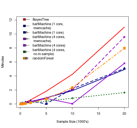
(a) Large sample sizes

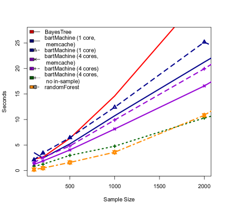
(b) Small sample sizes

Figure 1: Model creation times as a function of sample size for a number of settings of bartMachine, BayesTree and RandomForests. Simulations were run on a quad-core 3.4GHz Intel i5 desktop with 24GB of RAM running the Windows 7 64bit operating system.

We first note that Figure 1(a) demonstrates that the bartMachine model creation runtime is approximately linear in $n$ (without in-sample statistics computed). There is about a 30% speed-up when using four cores instead of one. The memcache enhancement should be turned off only with sample sizes larger than $n=20,000$. Noteworthy is the 50% reduction in time of constructing the model when not computing in-sample statistics. In-sample statistics are computed by default because the user generally wishes to see them. Also, for the purposes of this comparison, BayesTree models compute the in-sample statistics by necessity since the trees are not saved. The randomForest implementation becomes slower just after $n=1,000$ due to its reliance on a greedy exhaustive search at each node.

Figure 1(b) displays results for smaller sample sizes ($n\leq 2,000$) that are often encountered in practice. We observe the memcache enhancement provides about a 10% speed improvement. Thus, if memory is an issue, it can be turned off with little performance degradation.

3.2 Missing data in bartMachine

bartMachine implements a native method for incorporating missing data into both model creation and future prediction with test data. The details are given in Kapelner2013 but we provide a brief summary here.

There are a number of ways to incorporate missingness into tree-based methods (see Ding2010 for a review). The method implemented here is known as “Missing Incorporated in Attributes” (MIA, Twala2008, section 2) which natively incorporates missingness by augmenting the nodes’ splitting rules to (a) also handle sorting the missing data to the left or right and (b) use missingness itself as a variable to be considered in a splitting rule. Table 2 summarizes these new splitting rules as they are implemented within the package.

Implementing MIA into the BART procedure is straightforward. These new splitting rules are sampled uniformly during the GROW or CHANGE steps. For example, a splitting rule might be “$\boldsymbol{x}_{j}<c$ or $\boldsymbol{x}_{j}$ is missing.” To account for splitting on missingness itself, we create dummy vectors of length $n$ for each of the $p$ attributes, denoted $\boldsymbol{M}_{1},\ldots,\boldsymbol{M}_{p}$, which assume the value 1 when the entry is missing and 0 when the entry is present. The original training matrix is then augmented with these dummies, giving the opportunity to select missingness itself when choosing a new splitting rule during the grow or change steps. Note that this can increase the number of predictors by up to a factor of 2. We illustrate building a bartMachine model with missing data in Section LABEL:subsec:incorporating_missing_data. As described in Chipman2010, BART’s runtime increases negligibly in the number of covariates and this has been our experience using the augmented training matrix.

Table 2: The MIA choices for all attributes $j\in\left\{1,\ldots,p\right\}$ and all split points $x^{*}_{ij}$ where $i\in\left\{1,\ldots,n\right\}$ during a GROW or CHANGE step in bartMachine.

1:	If $x_{ij}$ is missing, send it $\longleftarrow$; if it is present and $x_{ij}\leq x^{*}_{ij}$, send it $\longleftarrow$, otherwise $\longrightarrow$.
2:	If $x_{ij}$ is missing, send it $\longrightarrow$; if it is present and $x_{ij}\leq x^{*}_{ij}$, send it $\longleftarrow$, otherwise $\longrightarrow$.
3:	If $x_{ij}$ is missing, send it $\longleftarrow$; if it is present, send it $\longrightarrow$.

3.3 Variable selection

Our package also implements the variable selection procedures developed in Bleich2014, which is best applied to data problems where the number of covariates influencing the response is small relative to the total number of covariates. We give a brief summary of the procedures here.

In order to select variables, we make use of the “variable inclusion proportions,” the proportion of times each predictor is chosen as a splitting rule divided by the total number of splitting rules appearing in the model (see Section 4.5 for more details). The variable selection procedure can be outlined as follows:

1. Compute the model’s variable inclusion proportions.

2. Permute the response vector, thereby breaking the relationship between the covariates and the response. Rebuild the model and compute the “null” variable inclusion proportions. Repeat this a number of times to create a null permutation distribution.

3. Three selection rules can be used depending on the desired stringency of selection:

   1. Local Threshold: Include a predictor $\boldsymbol{x}_{k}$ if its variable inclusion proportion exceeds the $1-\alpha$ quantile of its own null distribution.

   2. Global Max Threshold: Include a predictor $\boldsymbol{x}_{k}$ if its variable inclusion proportion exceeds the $1-\alpha$ quantile of the distribution of the maximum of the null variable inclusion proportions from each permutation of the response.

   3. Global SE Threshold: Select $\boldsymbol{x}_{k}$ if its variable inclusion proportion exceeds a threshold based from its own null distribution mean and SD with a global multiplier shared by all predictors.

The Local procedure is the least stringent in terms of selection and the Global Max procedure the most. The Global SE procedure is a compromise, but behaves more similarly to the Global Max. Bleich2014 demonstrate that the best procedure depends on the underlying sparsity of the problem, which is often unknown. Therefore, the authors include an additional procedure that chooses the best of these thresholds via cross-validation and this method is also implemented in bartMachine. As highlighted in Bleich2014, this method performs favorably compared to variable selection using random forests “importance scores”, which rely on the reduction in out-of-bag forecasting accuracy that occurs from shuffling the values for a particular predictor and dropping the out-of-bag observations down each tree. Examples of these procedures for variable selection are provided in Section LABEL:subsec:variable_selection_regression.

4 bartMachine Package Features for Regression

We illustrate the package features by using both real and simulated data, focusing first on regression problems.

4.1 Computing parameters

We first set some computing parameters. In this exploration, we allow up to 5GB of RAM for the Java heap and we set the number of computing cores available for use to 4.

R> options(java.parameters = "-Xmx5000m") R> library("bartMachine") R> set_bart_machine_num_cores(4)

The following Sections 4.2 – LABEL:subsec:variable_selection_regression use a dataset obtained from UCI (Bache2013). The $n=201$ observations are automobiles and the goal is to predict each automobile’s price from 25 features (15 continuous and 10 nominal), first explored by Kibler1989. This dataset also contains missing data. The following code loads the data. We omit missing data for now and we create a variable for the design matrix $\boldsymbol{X}$ and the response $\boldsymbol{y}$ which has already been log-transformed.

R> data(automobile) R> automobile = na.omit(automobile) R> y <- automobile$log_{p}riceR>X<-automobile;X$log_price <- NULL

4.2 Model building

We are now are ready to construct a bartMachine model. The default hyperparameters generally follow the recommendations of Chipman2010 and provide a ready-to-use algorithm for many data problems. Our hyperparameter settings are $m=50$, $\alpha=0.95$, $\beta=2$, $k=2$, $q=0.9$, $\nu=3$, and probabilities of the GROW / PRUNE / CHANGE steps is 28% / 28% /44%. We set the number of burn-in Gibbs samples to 250 and number of post-burn-in samples to 1,000. We default the missing data feature to be off. We default the covariates to be equally important a priori. Other parameters and their defaults can be found in the package’s online manual. Below is a default bartMachine model. Here, $\boldsymbol{X}$ denotes automobile attributes and $\boldsymbol{y}$ denotes the log price of the automobile.

R> bart_machine <- bartMachine(X, y) Building bartMachine for regression … evaluating in sample data…done

If one wishes to see more information about the individual iterations of the Gibbs sampler of Equation 3, the flag verbose can be set to “TRUE.” One can see more debug information from the Java program by setting the flag debug_log to true and the program will print to unnamed.log in the current working directory. In Figure 2 we inspect the model object to query its in-sample performance and to be reminded of the input data and model hyperparameters.

R> bart_machine bartMachine v1.1.1 for regression

training data n = 160 and p = 41 built in 1.7 secs on 4 cores, 50 trees, 250 burn-in and 1000 post. samples

sigsq est for y beforehand: 0.014 avg sigsq estimate after burn-in: 0.00794

in-sample statistics: L1 = 8.01 L2 = 0.65 rmse = 0.06 Pseudo-Rsq = 0.979 p-val for shapiro-wilk test of normality of residuals: 0.04584 p-val for zero-mean noise: 0.97575

Figure 2: The summary for the default bartMachine model built with the automobile data. Note that the “p-val for shapiro-wilk test of normality of residuals” is marginally less than 5%. Thus we conclude that the noise of Equation 1 is not normally distributed. Just as when interpreting the results from a linear model, non-normality implies we should be circumspect concerning bartMachine output that relies on this distributional assumption such as the credible and prediction intervals of Section 4.4.

Since the response was considered continuous, we employ bartMachine for regression. The dimensions of the design matrix are given. Note that we dropped 41 observations that contained missing data (which we will retain in Section LABEL:subsec:incorporating_missing_data). We then have a recording of the MSE for the OLS model and our average estimate of $\sigma^{2}_{e}$. We are then given in-sample statistics on error. Pseudo-$R^{2}$ is calculated via $1-SSE/SST$. Also provided are outputs from tests of the error distribution being mean centered and normal. In this case, we cannot conclude normality of the residuals using the Shapiro-Wilk test.

We can also obtain out-of-sample statistics to assess level of overfitting by using k-fold cross-validation. Using 10 randomized folds we find:

R> k_fold_cv(X, y, k_folds = 10) ………. $L1_{e}rr[1]21.64303\par$L2_err [1] 4.742511

$rmse[1]0.1721647\par$PseudoRsq [1] 0.8467881

The Pseudo-$R^{2}$ being lower out-of-sample versus in-sample suggests evidence that bartMachine is slightly overfitting (note also that the training sample during cross-validation is 10% smaller). This function also returns the $\hat{y}$ predictions as well as the vector of the fold indices (which are omitted above).

It may also be of interest how the number of trees $m$ affects performance. One can examine how out-of-sample predictions vary by the number of trees via

R> rmse_by_num_trees(bart_machine, num_replicates = 20)

and the output is shown in Figure 3.

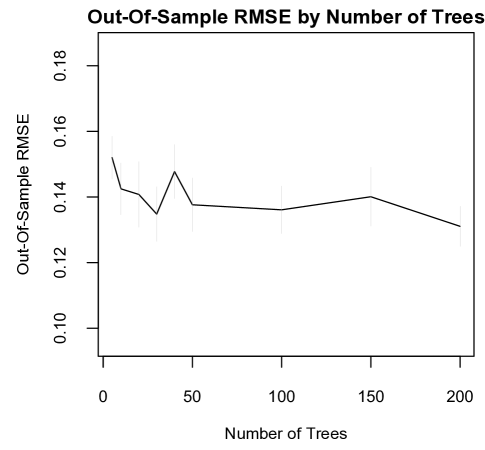
Figure 3: Out-of-sample predictive performance by number of trees

It seems that increasing $m>50$ does not result in any substantial increase in performance. We can now try to build a better bartMachine by grid-searching over a set of hyperparameter combinations, including $m$ (for more details, see BART-cv in Chipman2010). The default grid search is small and it can be customized by the user.

R> bart_machine_cv <- bartMachineCV(X, y) … bartMachine CV win: k: 2 nu, q: 3, 0.9 m: 200

This function returns the “winning” model, which is the one with lowest out-of-sample RMSE over a 5-fold cross-validation. Here, the cross-validated bartMachine model has slightly better in-sample performance (L1 = 8.18, L2 = 0.68 and Pseudo-$R^{2}=0.978$) as well as slightly better out-of-sample performance (L1 = 21.05, L2 = 4.40 and Pseudo-$R^{2}=0.858$) which were evaluated via:

R> k_fold_cv(X, y, k_folds = 10, k = 2, nu = 3, q = 0.9, num_trees = 200)

Predictions are handled with the predict function. Fits for the first seven rows are:

R> predict(bart_machine_cv, X[1 : 7, ]) [1] 9.494941 9.780791 9.795532 10.058445 9.670211 9.702682 9.911394

We also include a convenience method bart_predict_for_test_data that will predict and return out-of-sample error metrics when the test outcomes are known.

4.3 Assumption checking

The package includes features that assess the plausibility of the BART model assumptions. Checking the mean-centeredness of the noise is addressed in the summary output of Figure 2 and is simply a one-sample $t$-test of the average residual value against a null hypothesis of true mean zero. We assess both normality and heteroskedasticity via:

R> check_bart_error_assumptions(bart_machine_cv)

This will display a plot similar to Figure 4 which contains a QQ-plot (to assess normality) as well as a residual-by-predicted plot (to assess homoskedasticity). It appears that the errors are most likely normal and homoskedastic.

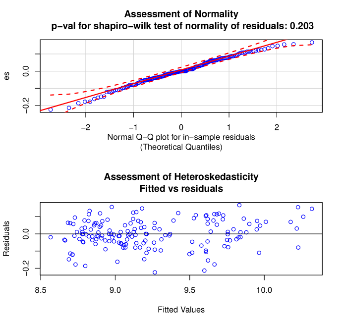
Figure 4: Test of normality of errors using QQ-plot and the Shapiro-Wilk test (top), residual plot to assess heteroskedasticity (bottom).

In addition to the model assumptions, BART requires convergence of its Gibbs sampler which can be investigated via:

R> plot_convergence_diagnostics(bart_machine_cv)

Figure 5 displays the plot which features four types of convergence diagnostics (each are detailed in the figure caption). It appears that the bartMachine model has been sufficiently burned-in.

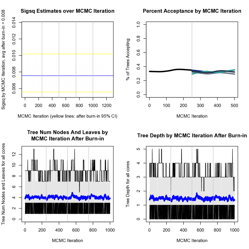
Figure 5: Convergence diagnostics for the cross-validated bartMachine model. Top left: $\sigma^{2}$ by MCMC iteration. Samples to the left of the first vertical grey line are burn-in from the first computing core’s MCMC chain. The four subsequent plots separated by grey lines are the post-burn-in iterations from each of the four computing cores employed during model construction. Top right: percent acceptance of Metropolis-Hastings proposals across the $m$ trees where each point plots one iteration. Points before the grey vertical line illustrate burn-in iterations and points after illustrate post burn-in iterations. Each computing core is colored differently. Bottom left: average number of leaves across the $m$ trees by iteration (post burn-in only where computing cores separated by vertical grey lines). Bottom right: average tree depth across the $m$ trees by iteration (post burn-in only where computing cores separated by vertical grey lines).

4.4 Credible intervals and prediction intervals

An advantage of BART is that if we believe the priors and model assumptions, the Bayesian probability model and corresponding burned-in MCMC iterations provide the approximate posterior distribution of $f\left(\boldsymbol{x}\right)$. Thus, one can compute uncertainty estimates via quantiles of the posterior samples. These provide Bayesian “credible intervals” which are intervals for the conditional expectation function, $\mathbb{E}\left[\boldsymbol{y}~{}|~{}\boldsymbol{X}\right]$.

Another useful uncertainty interval can be computed for individual predictions by combining uncertainty from the conditional expectation function with the systematic, homoskedastic normal noise produced by $\mathcal{E}$. This is accomplished by generating 1,000 samples (by defauilt) from the posterior predictive distribution and then reporting the appropriate quantiles.

Below is an example of how both types of intervals are computed in the package (for the 100th observation of the training data):

R> calc_credible_intervals(bart_machine_cv, X[100, ], ci_conf = 0.95) ci_lower_bd ci_upper_bd [1,] 8.725202 8.971687 R> calc_prediction_intervals(bart_machine_cv, X[100, ], pi_conf = 0.95) pi_lower_bd pi_upper_bd [1,] 8.631243 9.06353

Note that the prediction intervals are wider than the credible intervals because they reflect the uncertainty from the error term.

We can then plot these intervals in sample:

R> plot_y_vs_yhat(bart_machine_cv, credible_intervals = TRUE) R> plot_y_vs_yhat(bart_machine_cv, prediction_intervals = TRUE)

Figure 6(a) shows how our prediction fared against the original response (in-sample) with 95% credible intervals. Figure 6(b) shows the same prediction versus the original response plot now with 95% prediction intervals.

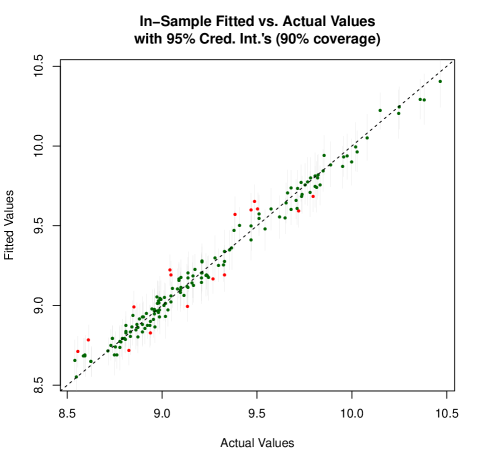
(a) Segments illlustrate credible intervals

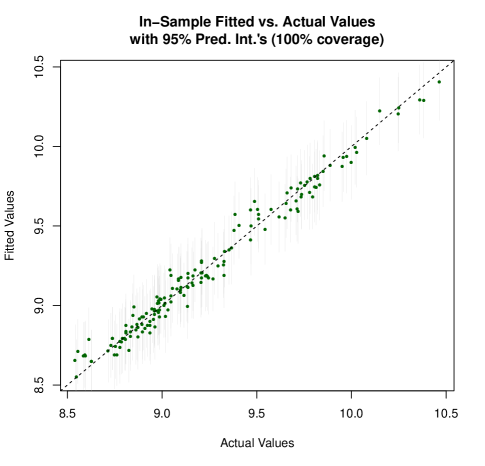
(b) Segments illlustrate prediction intervals

Figure 6: Fitted versus actual response values for the automobile dataset. Segments are 95% credible intervals (a) or 95% prediction intervals (b). Green dots indicate the true response is within the stated interval and red dots indicate otherwise. Note that the percent coverage in (a) is not expected to be 95% because the response includes a noise term.

4.5 Variable importance

After a bartMachine model is built, it is natural to ask the question: which variables are most important? This is assessed by examining the splitting rules in the $m$ trees across the post burn-in MCMC iterations which are known as “inclusion proportions” (Chipman2010). The inclusion proportion for any given predictor represents the proportion of times that variable is chosen as a spliting rule out of all splitting rules among the posterior draws of the sum-of-trees model. Figure 7 illustrates the inclusion proportions for all variables obtained via:

R> investigate_var_importance(bart_machine_cv, num_replicates_for_avg = 20)

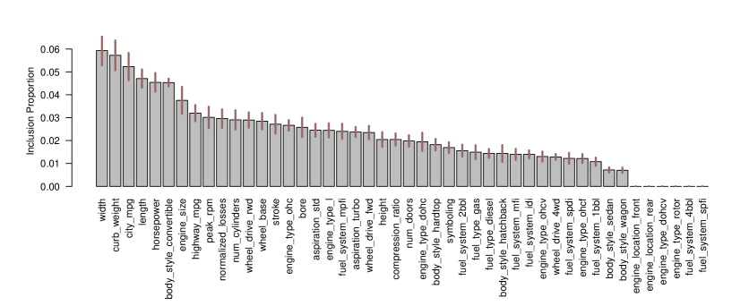
Figure 7: Average variable inclusion proportions in the cross-validated bartMachine model for the automobile data averaged over 100 model constructions to obtain stable estimates across many posterior modes in the sum-of-trees distribution (as recommended in Bleich2014). The segments atop the bars represent 95% confidence intervals. The eight predictors with inclusion proportions of zero feature identically one value (after missing data was dropped).

Selection of variables which significantly affect the response is addressed briefly in Section 3.3, examples are provided in Section LABEL:subsec:variable_selection_regression but for full treatment of this feature, please see Bleich2014.

4.6 Variable effects

It is also natural to ask: does $\boldsymbol{x}_{j}$ affect the response, controlling for other variables in the model? This is roughly analogous to the $t$-test in ordinary least squares regression of no linear effect of $\boldsymbol{x}_{j}$ on $\boldsymbol{y}$ while controlling for $\boldsymbol{x}_{-j}$. The null hypothesis here is the same but the linearity constraint is relaxed. To test this, we employ a permutation approach where we record the observed Pseudo-$R^{2}$ from the bartMachine model built with the original data. Then we permute the $\boldsymbol{x}_{j}$th column, thereby destroying any relationship between $\boldsymbol{x}_{j}$ and $\boldsymbol{y}$, construct a new duplicate bartMachine model from this permuted design matrix and record a “null” Pseudo-$R^{2}$. We then repeat this process to obtain a null distribution of Pseudo-$R^{2}$’s. Since the alternative hypothesis is that $\boldsymbol{x}_{j}$ has an effect on $\boldsymbol{y}$ in terms of predictive power, our $p$ value is the proportion of null Pseudo-$R^{2}$’s greater than the observed Pseudo-$R^{2}$, making our procedure a natural one-sided test. Note, however, that this test is conditional on the BART model and its selected priors being true, similar to the assumptions of the linear model.

If we wish to test if a set of covariates $A\subset\left\{\boldsymbol{x}_{1},\ldots,\boldsymbol{x}_{p}\right\}$ affect the response after controlling for other variables, we repeat the procedure outlined in the above paragraph by permuting the columns of $A$ in every null sample. We do not permute each column separately, but instead permute as a unit in order to perserve collinearity structure. This is roughly analogous to the partial $F$-test in ordinary least squares regression.

If we wish to test if any of the covariates matter in predicting $\boldsymbol{y}$, we simply permute $\boldsymbol{y}$ during the null sampling. This procedure breaks the relationship between the response and the predictors but does not alter the existing associations between predictors. This is roughly analogous to the omnibus $F$-test in ordinary least squares regression.

At $\alpha=0.05$, Figure LABEL:fig:cov_test_width demonstrates an insignificant effect of the variable width of car on price. Even though width is putatively the “most important” variable as measured by proportions of splits in the posterior sum-of-trees model (Figure 7), note that this is largely an easy prediction problem with many collinear predictors. Figure LABEL:fig:cov_test_body_style shows the results of a test of the putatively most important categorical variable, body style (which involves permuting the categories, then dummifying the levels to preserve the structure of the variable). We find a marginally significant effect ($p=0.0495$). A test of the top ten most important variables is convincingly significant (Figure LABEL:fig:cov_test_top_10). For the omnibus test, Figure LABEL:fig:cov_test_omnibus illustrates an extremely statistically significant result, as would be expected. The code to run these tests is shown below (output suppressed).

R> cov_importance_test(bart_machine_cv, covariates = c("width")) R> cov_importance_test(bart_machine_cv, covariates = c("body_style")) R> cov_importance_test(bart_machine_cv, covariates = c("width", "curb_weight", "city_mpg", "length", "horsepower", "body_style", "engine_size", "highway_mpg", "peak_rpm", "normalized