Primordial magnetic fields from a non-singular bouncing cosmology

Abstract

Although inflation is a natural candidate to generate the lengths of coherence of magnetic fields needed to explain current observations, it needs to break conformal invariance of electromagnetism to obtain significant magnetic amplitudes. Of the simplest realizations are the kinetically-coupled theories $f^{2}(\phi)F_{\mu\nu}F^{\mu\nu}$ (or $IFF$ theories). However, these are known to suffer from electric fields backreaction or the strong coupling problem. In this work we shall confirm that such class of theories are problematic to support magnetogenesis during inflationary cosmology. On the contrary, we show that a bouncing cosmology with a contracting phase dominated by an equation of state with $p>-\rho/3$ can support magnetogenesis, evading the backreaction/strong-coupling problem. Finally, we study safe magnetogenesis in a particular bouncing model with an ekpyrotic-like contracting phase. In this case we found that $f^{2}(\phi)F^{2}$-instabilities might arise during the final kinetic-driven expanding phase for steep ekpyrotic potentials.

I Introduction

One of the open problems of modern cosmology is to explain the origin of large scale magnetic fields in the structures of the universe. Indeed, during the last two decades the refinement of the experimental methods and the development of new ones allowed the confirmation of galactic and extragalactic microgauss magnetic fields. This was achieved through numerous observations measuresB1 . Moreover, from recent observations of secondary gamma rays produced by TeV-Blazars cosmic rays blazars , there were derived lower and upper limits for B-fields in voids regions: $1\times 10^{-17}G<B_{0}<3\times 10^{-14}G$.

The first theoretical explanation for galactic magnetic fields was the dynamo mechanism dynamo . The conventional dynamo is supported by classical magnetohydrodynamics and it works on galactic scales during the formation of the galaxy. However, this idea has lost ground for achieving galactic B-fields just by itself, and has been relegated to an amplification mechanism over primordial magnetic fields. The dynamo acts on galactic scales so in principle should only account for B-fields in galaxies. Thus, for explaining the presence of fields in the intergalactic medium, it needs additional mechanisms of ejection. Indeed, magnetic fields have been reported in the large-scale structure superclusters . Another important argument against the dynamo is the presence of microgauss fields in redshifted galaxies or galaxies in formation redshift . In these cases it is difficult to explain how such strong B-fields could have been generated in places where the dynamo had not enough time to act. Finally, the dynamo mechanism needs the presence of initial magnetic fields with minimum strengths and coherence lengths to be efficient.

In turn, this led much of the theoretical efforts to develop models of the early universe to account for the desired magnetogenesis. Indeed, in this subject, one can find many interesting large reviews with complete references therein reviews .

One of the many places where primordial magnetism is searched is during inflationary cosmology. The main feature of inflation is that it can naturally address the wide presence of magnetic fields, specially on the large scale. However, it is known that conformal symmetry of electromagnetism should be broken in order to obtain appreciable magnetic fields to the end of inflation. This was firstly done in Widrow88 by introducing new terms that coupled the electromagnetic field to the curvature of the universe. Another mechanism of breaking conformal invariance while keeping the gauge symmetry was proposed in Ratra92 and consisted in coupling the electromagnetic fields to a scalar field through $e^{\lambda\phi}F^{2}$. This last scenario was inspired by string theories of gravity Veneziano95 . In Fogli08 a coupling $R^{n}F^{2}$ was studied during inflation. Furthermore, in Martin07 a complete analysis was performed, with models inspired by particle physics. Besides, at that time, instabilities in the background dynamics risen by the backreaction of the gauge field were already considered. However, until the study Mukhanov09 , the strong coupling problem was ignored. Here it was realized that inflationary magnetogenesis scenarios, that evade the backreaction of electric fields, could not evade very large values of the effective coupling ’constant’ during its initial stage.

However, inflation is not the only early cosmological theory that generates the stretching of microphysical fluctuations to super-Hubble scales. One possible scenario is a bouncing cosmology Novello . Yet, contracting cosmological phases are known to suffer from BKL-chaos instability generated by anisotropies BKL . Indeed, their energy density grows as fast as $a^{-6}$, like a stiff fluid (with $w=1$). In order to avoid such instabilities, one needs in the Friedmann equations a stiffer component (with $w>1$) for the background universe. In particular, this is done by the ekpyrotic scenario ekpyrotic1 . There are many cosmological models inspired in such scenario, like cyclic cosmologies cyclic and the ”new ekpyrotic” cosmologies Ovrut07 [see ekpyrotic2 for a recent review]. Other realizations are many bounce , where new physics are required to provide the bounce, by violating the null energy condition. Particularly, in new ekpyrotic scenario the job is done by a ghost condensate phase Creminelli06 of the scalar field, yielding a non-singular bounce.

A previous study concerning early magnetogenesis from bouncing cosmologies is Salim0612 . However, they considered a background were the effective equation of state is $w=1$, thus it is not clear if the contracting phase is free of the anisotropy instability. Additionally, electromagnetic instabilities or backreaction were not studied. And finally, the coupling function $I(\omega)=e^{-2\omega}$ remains always well below unity for their parameters $\lambda\approx 0.07\sim 0.1$, thus yielding a strong-coupled regime.

The main objective of the present work is to identify the condition which determine the presence of the strong coupling/backreaction problem in a cosmological background. We start by considering an early background cosmological phase dominated by a constant equation of state $w$. Here we placed the $f^{2}F^{2}$ (or $IFF$) electromagnetic theory at a perturbative level. Initially, the coupling function is defined through a power-law $f\propto a^{n}$, where we call ’$n$’ the coupling parameter. This parametrization is useful since it leads to simple power-law spectrum for the electromagnetic field. Using this, we find a generalized parameter $\gamma=2n/(1+3w)$, that characterizes the dynamics of the electromagnetic modes and its spectrum. Next we considered the backreaction of electromagnetic fields. As already noted in previous works, we find that the branch safe from backreaction of the electric fields corresponds to $\gamma<0$. Here B-fields lead the spectrum of electromagnetic fields and make magnetogenesis efficient. However, the strong-coupled regime belongs to values $n>0$. Thus, one confirms that during inflation both problems cannot be simultaneously solved. Clearly, such a statement is done for the present $f^{2}F^{2}$ universality, without introducing any further assumptions (in particular in Sloth13 they considered low-scale inflation). Nevertheless, to simultaneously address both problems, one needs that $\gamma<0$ and $n<0$. We find that this will only happen for cosmological phases with $w>-1/3$.

This condition motivated the second part of our work. We searched for magnetogenesis in an early cosmological phase with $w>-1/3$. This phase should have the property of stretching microphysical fluctuations to super-Hubble scales, similarly to inflation. Such condition can only be achieved by contracting phases ($\dot{a}<0$ or $H<0$) given that their comoving Hubble sphere shrinks like $(a|H|)^{-1}\propto a^{(1+3w)/2}$ (for $w>-1/3$).

We used the background cosmology developed by Yi-Fu Cai, et.al. in Bran1206 as an example to study the production of magnetic fields. This model addresses the almost scale invariant spectrum of primordial inhomogeneities by using curvature perturbations instead of entropy perturbations, as is done in the usual ekpyrotic scenarios. This model is a realization of the Matter-Bounce scenarios Bran0904 that includes an early contracting phase with an ekpyrotic-like equation of state ($w>1$). Indeed, this contracting phase is refereed as the ekpyrotic phase. Also, in Bran1301 it was studied, at the linear level, that such a realization was stable against chaos from anisotropy during the bounce. This model was further extended to a two-field picture in Bran1305 . Moreover, very recently this was confirmed at the nonperturbative level Steinhardt1308 , but showing some fine-tunning problems.

We checked that this model is free from the backreaction/strong coupling problem during the contracting phase. Indeed, the weak coupled regime persist during the whole dynamics. However, we find that instabilities might arise during the final fast-roll expanding phase. This backreaction could be severe if the fast-roll lasts for too long when the ekpyrotic potential is very steep and asymmetric. Yet, for weaker ekpyrotic phases stability is recovered.

The paper is organized as follows. In SectionII we study the evolution of electromagnetic fields kinetically-coupled to a scalar field by $f^{2}(\phi)F^{2}$. We assume the scalar field dominates the Einstein equations, thus the electromagnetic field is effectively coupled to the background dynamics. We study the conditions on the parameters where the backreaction/strong coupling problem appears. In SectionIII we apply these results to a specific example that deploys a bounce. It starts from an early ekpyrotic contracting phase and then bounces to a fast-roll expanding period. We set initial conditions to the electromagnetic field during the contracting phase. Then, we study the evolution of these modes through the different phases. In doing so, we introduce an specific model for the coupling of the $e^{\lambda\phi}$ type. This is consistent with the background dynamics and the power-law behavior. Next we kept the track of the levels of backreaction during the contracting an the expanding phase. Finally in SectionIV we give our conclusions. In this article we use Natural units: $c=\hbar=k_{B}=1$.

II $f(\phi)^{2}F^{2}$ Electromagnetic fields in a cosmological background

We adopt a simple model where the electromagnetic field is coupled to a scalar field that dominates the energy density of the universe. This coupling is referred to as a $f(\phi)^{2}F^{2}$ or $IFF$-class models. Indeed, as $\phi$ varies with time this implies that, effectively, we are introducing a time-dependent coupling ’constant’ $e_{\mathrm{eff}}$, given by the inverse of the coupling function, $e_{\mathrm{eff}}=ef^{-1}$. This kind of scenarios had been extensively studied during an inflationary phase to account for the generation of primordial magnetic fields. However, they have proven to suffer two kinds of troubles: the strong coupling problem and the backreaction problem Mukhanov09 . Even worse, where one can be solved the other emerges.

Other realizations were kinetic couplings have been recently used are for: anisotropic-inflation or gauge-inflation Sodareport , preheating of the inflaton with a U(1) gauge field Caldwell13 and non-Gaussianity features Bnongaussian .

We shall start by studying how the fluctuation modes of the gauge field evolve in a cosmological background with a constant equation of state $p=w\rho$. In doing so, we shall find a simple relation between $w$, the spectrum of magnetic fields and the backreaction/strong coupling problem.

We will adapt part of the derivations used in Martin07 for inflation, and refer the reader there for detailed derivations.

II.1 Electromagnetic perturbations coupled to the background dynamics

Consider the action of a gauge $U(1)$ field (which we shall identify with ’the electromagnetic field’) coupled to a scalar field $\phi$, as

$$S_{\mathrm{em}}=-\frac{1}{4}\int d^{4}x\sqrt{-g}f^{2}(\phi)F_{\mu\nu}F^{\mu\nu},$$ (1)

with the electromagnetic tensor $F_{\mu\nu}=\partial_{\mu}A_{\nu}-\partial_{\nu}A_{\mu}$. Here the vector potential has dimensions of mass $[A_{\mu}]=M$. The coupling function $f(\phi)$ is in this sense dimensionless. The equations of motion for $A_{\mu}$ are

$$\partial_{\mu}[\sqrt{-g}f^{2}(\phi)F^{\mu\nu}]=0.$$ (2)

We assume that the gauge fields are small enough so that the background dynamics are entirely determined by the homogeneous scalar field, thus we consider an homogeneous and isotropic FRWL space-time,

$$ds^{2}=g_{\mu\nu}dx^{\mu}dx^{\nu}=-dt^{2}+a^{2}(t)d\mathbf{x}^{2}=a^{2}(\tau)(-d\tau^{2}+d\mathbf{x}^{2}).$$ (3)

In this the last expression we used conformal time $\tau=\int a^{-1}dt$. With the coulomb gauge $A_{0}=\partial_{i}A_{i}=0$, we completely fix the gauge freedom. The vector field is promoted through canonical quantization to an operator with Fourier decomposition

$$A_{i}(\tau,\mathbf{x})=\int\frac{d^{3}k}{(2\pi)^{3/2}}\sum_{\lambda=1}^{2}\left[\epsilon_{i\lambda}(\mathbf{k})b_{\lambda}(\mathbf{k})A(\tau,k)e^{i\mathbf{k}\cdot\mathbf{x}}+h.c.\right].$$ (4)

Using the mode definition $u_{k}(\tau,k)=a(\tau)A(\tau,k)$, we obtain a damped harmonic oscillator equation

$$u_{k}^{\prime\prime}+2\frac{f^{\prime}}{f}u^{\prime}_{k}+k^{2}u_{k}=0,\hskip 28.45274pt\ddot{u}_{k}+\left(H+2\frac{\dot{f}}{f}\right)\dot{u}_{k}+\frac{k^{2}}{a^{2}}u_{k}=0,$$ (5)

with time-dependent damping. In particular, for the value $f=1=cte$ one recovers the conformal Maxwell theory. This equation may also be written as

$$(fu_{k})^{\prime\prime}+\left(k^{2}-\frac{f^{\prime\prime}}{f}\right)(fu_{k})=0.$$ (6)

Thus, sometimes is useful to consider the redefined modes ${\cal A}_{k}\equiv fu_{k}$. With the aid of which we can identify short wavelength modes as those for which $k^{2}\gg f^{\prime\prime}/f$. Indeed, these solutions behave like plane waves in Minkowski space, addressing the vacuum initial conditions

$$u_{k}(\tau)\rightarrow\frac{1}{f\sqrt{2k}}e^{-ik\tau},\hskip 28.45274pt{\cal A}_{k}(\tau)\rightarrow\frac{1}{\sqrt{2k}}e^{-ik\tau}.$$ (7)

On the other side, when this modes overpass the Hubble scale they eventually get into the long wavelength regime $k^{2}\ll f^{\prime\prime}/f$, where the fields stop oscillating and have the solution

$$u_{k}(\tau)\rightarrow c_{1}(k)+c_{2}(k)\int\frac{d\tau}{f^{2}},\hskip 28.45274pt{\cal A}_{k}(\tau)\rightarrow c_{1}(k)f+c_{2}(k)f\int\frac{d\tau}{f^{2}}.$$ (8)

For $u_{k}$, the solution consists in a constant mode and a time-dependent mode. We shall assume a power-law behavior,

$$f(a)=f_{\star}\left(\frac{a}{a_{\star}}\right)^{n},$$ (9)

where ’$n$’ is the coupling parameter. Such a choice is motivated by simplicity, as we shall see, this form gives a simple power-law for the electromagnetic field spectrum. In this sense, any simple model that has a simple power-law electromagnetic field spectrum will be consistent with this parametrization. Moreover, this choice also considers exponential forms as originally introduced in Ratra92 . Defining the equation of state of the universe as $p=w\rho$, we obtain that

$$\left\{\begin{array}[]{ll}a\propto t^{\frac{2}{3(w+1)}},&\hbox{$w\neq-1$;}\\ a\propto e^{H_{I}t},&\hbox{$w=-1$.}\\ \end{array}\right.$$ (12)

This is sufficient to yield the solutions

$$u_{k}(\tau) \simeq c_{1}(k)+c_{2}(k)\left(\frac{a}{a_{\star}}\right)^{r},\hskip 28.45274ptr=-2n+\frac{1}{2}(1+3w)$$ (13)

$${\cal A}_{k}(\tau) \simeq c_{1}(k)\left(\frac{a}{a_{\star}}\right)^{n}+c_{2}(k)\left(\frac{a}{a_{\star}}\right)^{r+n},$$

the first has a constant mode $c_{1}(k)$ and a time-dependent mode with pivot amplitude $c_{2}(k)$.

During de Sitter inflation we have $w=-1$ that yields on the solution for the vector modes (13) an exponent given by

$$r^{(in)}=-2n-1.$$ (14)

If now we turn to an ekpyrotic phase with a equation of state $w=-1+2/(3q)$, we obtain an exponent

$$r^{(ek)}=-2n-1+\frac{1}{q}.$$ (15)

This last expression can also be identified with slow-roll inflation. Indeed, the slow-roll parameter is $\epsilon=1/q=3(1+w)/2$ for $w\approx-1$ or $q\gg 1$. Conversely, this is the same fast-roll parameter for ekpyrosis as $w\gg 1$ and then $q\ll 1$. This is a manifestation of the duality (at linear level) between inflation and ekpyrosis Turok0403 .

We start by noticing that $f^{\prime}/f=n{\cal H}$, where ${\cal H}=a^{\prime}/a=\dot{a}$ is the conformal Hubble parameter. Furthermore, the scale factor is related to conformal time $\tau=\int a^{-1}dt$, in terms of the equation of state through

$$\frac{a}{a_{\star}}=\left(\frac{\tau}{\tau_{\star}}\right)^{\frac{2}{1+3w}},$$ (16)

and the Hubble parameter

$${\cal H}=aH=\frac{2}{1+3w}\tau^{-1}.$$ (17)

It is convenient to introduce a new parameter that depends both on $n$ and $w$,

$$\gamma=\frac{2n}{1+3w},$$ (18)

with the aid of which the mode equation gets simplified

$${u_{k}}^{\prime\prime}+\frac{2\gamma}{\tau}{u_{k}}^{\prime}+k^{2}u_{k}=0,\hskip 28.45274pt{\cal A}_{k}^{\prime\prime}+\left[k^{2}-\frac{\gamma(\gamma-1)}{\tau^{2}}\right]{\cal A}_{k}=0.$$ (19)

One can either solve any of these last equations, and the exact solution is given in terms of Bessel functions

$${\cal A}_{k}(x)=x^{\frac{1}{2}}\left[d_{1}(k){\cal H}^{(1)}_{\frac{1}{2}-\gamma}(x)+d_{2}(k){\cal H}^{(2)}_{\frac{1}{2}-\gamma}(x)\right],$$ (20)

with $x=-k\tau$. We have used Hankel functions for convenience, in this sense the initial vacuum conditions [see eq.(7)] are trivially achieved for the second Hankel function ${\cal H}^{(2)}_{\gamma-\frac{1}{2}}(x\rightarrow\infty)\rightarrow x^{-1/2}e^{-ix}$. Thus, we obtain

$$d_{1}(k) = 0,$$ (21)

$$d_{2}(k) = \sqrt{\frac{\pi}{4k}}e^{i\frac{\pi}{2}(\gamma-1)}.$$ (22)

On the other side, the long wavelength regime for Hankel functions may be computed from the asymptotic form of First Kind Bessel functions $J_{\mu}(x)\propto x^{\mu}$. Moreover, we use that ${\cal H}^{(2)}_{\mu}(x)=i\csc(\alpha\pi)[J_{-\mu}(x)-e^{i\pi\mu}J_{\mu}(x)]$. The expression for $u_{k}$ is then,

$$u_{k}(x)=\frac{{\cal A}_{k}}{f}=\frac{b_{(\gamma)}}{f\sqrt{k}}x^{\gamma}+\frac{b_{(1-\gamma)}}{f\sqrt{k}}x^{1-\gamma},$$ (23)

with the function

$$b_{(\gamma)}=\frac{\pi^{\frac{1}{2}}e^{i\frac{\pi\gamma}{2}}}{2^{\frac{1}{2}+\gamma}\cos{(\gamma\pi)}\Gamma\left(\frac{1}{2}+\gamma\right)}.$$ (24)

With this considerations one can determine exactly the constants of the solution (13), that they show to be

$$c_{1}(k) = b_{(\gamma)}\left(\frac{2}{1+3w}\right)^{\gamma}\frac{1}{f_{\star}{k}^{1/2}}\left(\frac{k}{a_{\star}H_{\star}}\right)^{\gamma},$$ (25)

$$c_{2}(k) = b_{(1-\gamma)}\left(\frac{2}{1+3w}\right)^{1-\gamma}\frac{1}{f_{\star}{k}^{1/2}}\left(\frac{k}{a_{\star}H_{\star}}\right)^{1-\gamma},$$

where we have used (17) to change from the conformal pivot time $\tau_{\star}$ to $a_{\star}H_{\star}$. Cleared up the constants, we can apply a specific background model that fixes the value of $w$, and by using (16), (17) and (18) we are only left to determine the coupling function parameter $n$. We shall either use $b_{(\gamma)},b_{(1-\gamma)}$ or $c_{1}(k),c_{2}(k)$ in convenience to alleviate the algebraic manipulations and notation. Another important quantity is the time derivative of the $u_{k}$ modes. Not only it defines the electric energy density, but the matching conditions as well. However, care should be taken because the $c_{1}$-term is constant and so, when deriving, it would just remain a contribution from the $c_{2}$-term. Yet, one has to consider the next order in the power series of the Bessel $J_{\mu}(x)$, that goes like $\sim x^{2+\mu}$. Thus, we arrive at the expression,

$$\dot{u}_{k}=\left(\frac{1+3w}{2}\right)H\left[\frac{e_{(-\gamma)}}{f\sqrt{k}}x^{\gamma+2}+\frac{e_{(1+\gamma)}}{f\sqrt{k}}x^{1-\gamma}\right],$$ (26)

where it has been used that $\dot{x}/x=(1+3w)H/2$ and the function

$$e_{(\gamma)}=-\frac{b_{(-\gamma)}}{1-2\gamma}.$$ (27)

II.2 Electromagnetic energy density

For the determination of the magnetic fields amplitude and the effects of backreaction that may occur, we shall compute the total electromagnetic energy density stored at a certain scale $L=2\pi k^{-1}$. The energy density is defined through the vacuum expectation value of the time-time component of the stress tensor as $\rho_{\mathrm{em}}\equiv-\langle 0|{T}^{0}_{0}|0\rangle$. The stress tensor of the fields is determined by

$$T_{\mu\nu}\equiv-\frac{2}{\sqrt{-g}}\frac{\delta S_{\mathrm{em}}}{\delta g^{\mu\nu}}=-f^{2}(\phi)\left({F_{\mu}}^{\alpha}F_{\alpha\nu}+\frac{1}{4}g_{\mu\nu}F_{\alpha\beta}F^{\alpha\beta}\right).$$ (28)

We could further identify an electric and magnetic energy densities. But first we need to define electric and magnetic fields for relativistic observers with velocity $u^{\alpha}$,

$$E_{\mu}=u^{\nu}F_{\mu\nu},\hskip 28.45274ptB_{\mu}=\frac{1}{2}\eta_{\mu\nu\alpha\beta}F^{\nu\alpha}u^{\beta},$$ (29)

where $\eta_{\mu\nu\alpha\beta}=\sqrt{-g}\varepsilon_{\mu\nu\alpha\beta}$ is the space volume totally antisymmetric tensor related to the Levi-Civita symbol in 4D. Therefore, for a comoving observer $u^{\alpha}=(1,\mathbf{0})$, in cosmic time coordinates, one obtains an electric field $E_{i}=-\dot{A}_{i}$ and a magnetic field $B_{i}=a^{-1}\varepsilon_{ijk}\partial_{j}A_{k}$; both are written in the usual 3D Euclidean notation (where the metric tensor is the Kronecker Delta function $\delta_{ij}$).

With the above definitions it is easy to see that

$$T_{0}^{0}=-\frac{f^{2}}{2a^{2}}\left(|\vec{E}|^{2}+|\vec{B}|^{2}\right).$$ (30)

where $|\vec{E}|^{2}=\sum_{i=1}^{3}E_{i}^{2}=a^{2}E_{\mu}E^{\mu}$ and $|\vec{B}|^{2}=\sum_{i=1}^{3}B_{i}^{2}=a^{2}B_{\mu}B^{\mu}$. This last expression is written in cosmic time coordinates. One can pass to conformal coordinates, but the electric field changes by a factor $a$, then $\vec{\cal E}=-\partial_{\tau}\vec{A}=a\vec{E}$. The energy density of magnetic fields stored at a given scale $L=2\pi/k$ is

$$\frac{d\rho_{B}}{d\ln k}=\frac{f^{2}}{2\pi^{2}}\frac{k^{5}}{a^{4}}|u_{k}|^{2}.$$ (31)

While the energy density of electric fields at a given scale is

$$\frac{d\rho_{E}}{d\ln k}=\frac{f^{2}}{2\pi^{2}}\frac{k^{3}}{a^{2}}|\dot{u}_{k}|^{2}.$$ (32)

Now we need to calculate the quadratic quantities $|u^{(ek)}_{k}|^{2}$ and $|\dot{u}^{(ek)}_{k}|^{2}$, so as to determine the magnetic and electric densities energies per unit $k$. A direct calculation using the solution (13) or (23) yields,

$$|u_{k}|^{2} = |c_{1}(k)|^{2}+|c_{2}(k)|^{2}\left(\frac{a}{a_{\star}}\right)^{2r}+\left[c_{1}(k)c_{2}^{\ast}(k)+c_{1}^{\ast}(k)c_{2}(k)\right]\left(\frac{a}{a_{\star}}\right)^{r}$$ (33)

$$= \frac{1}{f^{2}k}\left[|b_{(\gamma)}|^{2}x^{2\gamma}+|b_{(1-\gamma)}|^{2}x^{2-2\gamma}+(b_{(\gamma)}b_{(1-\gamma)}^{\ast}+b_{(\gamma)}^{\ast}b_{(1-\gamma)})x\right].$$

The magnetic energy density on super Hubble scales ($x\ll 1$) is well approximated by

$$\frac{d\rho_{B}}{d\ln k}=\frac{H^{4}}{2\pi^{2}}\left(\frac{1+3w}{2}\right)^{4}\left\{\begin{array}[]{ll}|b_{(\gamma)}|^{2}(-k\tau)^{4+2\gamma},&\gamma<\frac{1}{2}\\ |b_{(1-\gamma)}|^{2}(-k\tau)^{6-2\gamma},&\gamma>\frac{1}{2}\\ \end{array}\right.$$ (36)

It is worth noticing that for a given spectral index there are two possible values of $\gamma$. For example, if we seek for scale invariant magnetic fields, then this is achieved for $\gamma=3$, that implies $n_{B}^{(2)}=6-2\gamma=0$. But, also for $\gamma=-2$, which yields $n_{B}^{(1)}=4+2\gamma=0$. Yet, one of this values may belong to the strong-coupled regime and the other to the weak-coupled regime. In the next we shall compare this possibilities between inflation and ekpyrosis.

But first, it remains the determination of the electric energy density per unit scale, that is defined through $\dot{u}_{k}$. Using the solution (26) in eq. (32) we get

$$\frac{d\rho_{E}}{d\ln k}=\frac{H^{4}}{2\pi^{2}}\left(\frac{1+3w}{2}\right)^{4}\left\{\begin{array}[]{ll}|e_{(-\gamma)}|^{2}(-k\tau)^{6+2\gamma},&\gamma<-\frac{1}{2}\\ |e_{(1+\gamma)}|^{2}(-k\tau)^{4-2\gamma},&\gamma>-\frac{1}{2}\\ \end{array}\right.$$ (37)

Similarly as the magnetic case, there are to possible values of $\gamma$ that yield the same spectrum.

One important observation about the last expressions (36) and (37) is that for a given value of $\gamma$ one of the terms will lead the spectrum, whereas the other in general will not be the immediate in sub-leading order (unless $|\gamma|<1/2$). For example, if we take the value $\gamma=-1$ the leading B-spectrum is $n_{B}^{(1)}=2$. On the other side, the other term gives a value $n_{B}^{(2)}=8$ that it is not the next to leading order contribution. Indeed, there are many terms before it, some of which are obtained by going to orders $k^{2}$ and $k^{4}$ starting from $n_{B}^{(1)}$ and others by considering the cross terms between $c_{1}(k)$ and $c_{2}(k)$. This situation is detailed in the right panel of Fig.(1). Here we plotted the first contributions in the spectrum from the electric and the magnetic fields. Notice how the subleading contributions of electric and magnetic fields will overlap. Additionally, the horizontal lines corresponds to the cross terms contribution that start from the lower B and E-spectrum $n_{BE}^{\mathrm{(cross)}}=5$, to higher. Beside, on the left panel, we only kept the leading contribution of them. The leading spectrum of each is defined in two ’branches’ of $\gamma$, this was previously obtained in Martin07 .

Finally, a crucial observation is that for $\gamma>0$ the E-spectrum leads with respect to the B-spectrum. Then, in this region one obtains electrogenesis, since most of the energy is given to electric fields in larger scales. For $\gamma\geq 1/2$ the B-spectrum is blue tilted respect to E as $n_{B}=n_{E}+2$. When one searches at inflation for the generation of magnetic fields in large scales, this region, $\gamma>0$, is associated with strong backreaction Mukhanov09 . In particular, interesting B-spectra are those close to scale invariance, $n_{B}\sim 0$. In this case, one gets a red-tilted spectrum for electric fields $n_{E}\sim-2$. In the middle, the value $\gamma=0$ yields blue magnetic and electric fields with the same index: $n_{B}=n_{E}=4$. Of course, this corresponds to the case $f=1=cte$, yielding the usual electromagnetic fields energy density that decays like $a^{-4}$. On the other side, the negative semiplane $\gamma<0$ has a red tilted B-spectrum with respect to E-fields. Moreover, for $\gamma<-1/2$ the red tilt is constant $n_{E}=n_{B}+2$. Therefore, this region should be identified to produce magnetogenesis. The value $\gamma=-2$ yields scale invariant B-fields and a blue electric field with $n_{E}=2$.

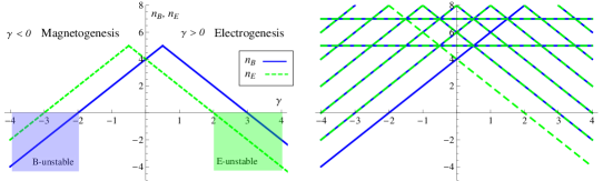
Figure 1: Left panel: the leading spectral contributions from the electric fields (green dashed line) and the magnetic fields (blue line) versus $\gamma$. Right panel: the overlap of sub-leading $E$ and $B$-spectral indexes.

II.3 Unstable growth of electromagnetic perturbations

When writing the Friedmann equations one should be aware that problems can arise if the perturbations of the vector field can grow to energy levels comparable to the background. Indeed, electromagnetic fields could generate serious deviations of isotropy, given that their anisotropy is of the same order of isotropy. In this sense, for the model to be successful it should control its backreaction in the cosmological scales.

To consider backreaction we have to sum the collective contribution of all the modes that reach the long wavelength regime and have common initial sub-horizon conditions. Whereas short wavelengths modes that remain below $(aH)^{-1}$ are renormalized at the leading order.

$$\rho_{E}+\rho_{B}=\int_{a_{i}H_{i}}^{aH}\frac{dk}{k}\left[\frac{d\rho_{E}}{d\ln k}+\frac{d\rho_{B}}{d\ln k}\right]$$ (38)

Next we compare the energy densities $\rho_{B}$ and $\rho_{E}$ with the background energy density $\rho_{T}=\frac{3}{8\pi}m_{pl}^{2}H^{2}$, obtaining the ratios

$$\Omega_{B}^{(1)}\equiv\frac{\rho_{B}^{(1)}}{\rho_{T}}=\frac{H^{2}}{m_{pl}^{2}}\frac{4|b(\gamma)|^{2}}{\pi}\left|\frac{2}{1+3w}\right|^{2\gamma}\times$$ (39)

$$\left\{\begin{array}[]{ll}\frac{1}{4+2\gamma}\left[1-e^{-(4+2\gamma)N(t)}\right],&\hbox{$\gamma\neq-2$;}\\ N(t),&\hbox{$\gamma=-2$.}\\ \end{array}\right.$$ (41)

where we have used $N(t)\equiv\ln\left(\frac{a(t)H(t)}{a_{i}H_{i}}\right)$ that accounts for the number of e-folds measured from a particular time $t_{i}$, when we have a variable $H$. In a similar way we find that

$$\Omega_{B}^{(2)}\equiv\frac{\rho_{B}^{(2)}}{\rho_{T}}=\frac{H^{2}}{m_{pl}^{2}}\frac{4|b(1-\gamma)|^{2}}{\pi}\left|\frac{2}{1+3w}\right|^{2-2\gamma}\times$$ (42)

$$\left\{\begin{array}[]{ll}\frac{1}{6-2\gamma}\left[1-e^{-(6-2\gamma)N(t)}\right],&\hbox{$\gamma\neq 3$;}\\ N(t),&\hbox{$\gamma=3$.}\\ \end{array}\right.$$ (44)

The label $(1)$ or $(2)$ refers to the $n_{B}^{(1)}$ and $n_{B}^{(2)}$ respectively. We also compute the relative electric energy density

$$\Omega_{E}^{(1)}\equiv\frac{\rho_{E}}{\rho_{T}}=\frac{H^{2}}{m_{pl}^{2}}\frac{4|e(-\gamma)|^{2}}{\pi}\left|\frac{2}{1+3w}\right|^{2\gamma}\times$$ (45)

$$\left\{\begin{array}[]{ll}\frac{1}{6+2\gamma}\left[1-e^{-(6+2\gamma)N(t)}\right],&\hbox{$\gamma\neq-3$;}\\ N(t),&\hbox{$\gamma=-3$.}\\ \end{array}\right.$$ (47)

$$\Omega_{E}^{(2)}\equiv\frac{\rho_{E}}{\rho_{T}}=\frac{H^{2}}{m_{pl}^{2}}\frac{4|e(1+\gamma)|^{2}}{\pi}\left|\frac{2}{1+3w}\right|^{2-2\gamma}\times$$ (48)

$$\left\{\begin{array}[]{ll}\frac{1}{4-2\gamma}\left[1-e^{-(4-2\gamma)N(t)}\right],&\hbox{$\gamma\neq 2$;}\\ N(t),&\hbox{$\gamma=2$.}\\ \end{array}\right.$$ (50)

For the model to be free of backreaction of the electromagnetic field, one needs that the last ratios remain well below unity during the whole dynamics, $\Omega_{B}+\Omega_{E}\ll 1$.

From the last ratios we can identify that there will be two types of instabilities. One produced by electric fields ($\gamma>2$) and the other by magnetic fields ($\gamma<-2$) see left panel of Fig.1). This happens essentially when the leading spectral index (E or B) becomes negative or red-tilted. In that case the exponentials factors grow with $N$.

II.4 The inflationary phase: $w\simeq-1$

Lets adopt the last derivations for the simplest inflationary case: de Sitter inflation. Indeed, the generalization to a slow-rolling model should be immediate. Here, we have $w=-1$ and the Hubble parameter is constant $H=H_{I}$. In this case we obtain from the parameter (18) the value

$$\gamma^{(\mathrm{in})}=-n$$ (51)

Thus, the solution [see eq.(13)] for the modes is $u_{k}^{(\mathrm{in})}=c_{1}^{(\mathrm{in})}(k)+c_{2}^{(\mathrm{in})}(k)\left(\frac{a}{a_{f}}\right)^{-2n-1}$ with the constants (25) for values $\gamma=-n$ and $w=-1$. Furthermore, the spectra of electric and magnetic fields are defined by the spectral indexes

$$n_{B}=\left\{\begin{array}[]{ll}n_{B}^{(1)}=4-2n,&n>-\frac{1}{2}\\ n_{B}^{(2)}=6+2n,&n<-\frac{1}{2}\\ \end{array}\right.,\hskip 28.45274ptn_{E}=\left\{\begin{array}[]{ll}n_{E}^{(1)}=6-2n,&n>\frac{1}{2}\\ n_{E}^{(2)}=4+2n,&n<\frac{1}{2}\\ \end{array}\right.$$ (52)

For the generation of large scale magnetic fields one pursues almost scale invariant magnetic fields, more efficient to concentrate energy on larger scales. Nevertheless, red-tilted spectra, as we have seen, are likely to develop backreaction.

One obtains scale-invariant magnetic fields, $n_{B}=0$, for $\gamma=3$ and $\gamma=-2$. These corresponds with the values $n=-3$ and $n=2$, respectively. Yet, the value $n=-3$ leaves us with a red-tilted electric field $n_{E}=-2$, while for $n=2$, one gets a blue-tilt $n_{E}=2$. This, in turn, means that the values close to $n=-3$ look more problematic and inefficient, since most of the energy that the mechanism carries to large scales goes to E-fields rather than to B-fields. Indeed, trying to keep controlled the levels of backreaction left us with very little magnetic fields ($10^{-32}$G) to the end of inflation ($N=75$), insufficient to account for minimum levels needed by dynamo mechanisms Mukhanov09 .

On the contrary, the value $n=2$ is safe from this drawback. However, values $n>0$ belong to the strong-coupled regime. In particular for $n=2$ and $N=75$, and given that to the end of inflation $f_{\emph{end}}\sim 1$, the inverse of the coupling function is of order $e^{150}\sim 10^{64}$ at the beginning of the inflationary period, and the theory becomes non-perturbative and all our analysis breaks down.

II.5 The backreaction/strong-coupling problem: expansion or contraction?

Lets check expression (18), this parameter $\gamma$ defines the spectrum of the electromagnetic field in a background with an equation of state $w$ and with a coupling parameter $n$. We can write $n/\gamma=(1+3w)/2$. This expression is also present in the relation for the comoving Hubble radius

$$(aH)^{-1}\propto a^{\frac{1+3w}{2}}$$ (53)

Thus, if the universe expands ($\dot{a}>0$) we have three cases. When $w>-1/3$ the strong energy condition (SEC) is achieved and then the universe decelerates ($\ddot{a}<0$) and the Hubble radius grows. The Big-Bang epochs dominated by ordinary matter ($w\gtrsim 0$) belongs to this case. For $w<-1/3$ the SEC is violated and the universe has an accelerated expansion with a shrinking Hubble sphere. Slow-roll inflation for which $w\simeq-1$, belongs to these class. Furthermore, the value $w=-1/3$ yields a constant Hubble sphere. For a contracting universe ($\dot{a}<0$) the situation inverts. When $w<-1/3$, the universe decelerates its contraction rate and the comoving Hubble length grows with time. While, for $w>-1/3$, the universe speeds up its contraction making the Hubble sphere shrink. Finally, when $w=-1/3$, the Hubble sphere remains constant.

Returning to the parameter $\gamma$, we see that (independently if the universe is expanding or contracting), when $w<-1/3$ the signs of $n$ and $\gamma$ will be inverted. Then, if we want to remain with a dominant B-spectrum, red-tilted with respect to the E-spectrum, we require that $\gamma<0$. This automatically leaves us with a value $n>0$, say, the strong-coupled regime [see Fig.(2)]. We find that $(f^{2}F^{2})-$class models in any expanding accelerated background ($w<-1/3$) cannot simultaneously avoid the backreaction and strong-coupling problems.

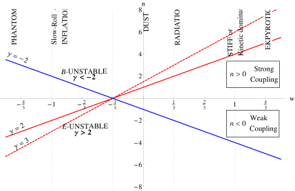
Figure 2: The coupling parameter $n$ vs. the equation of state parameter $w$. The dotted-red line corresponds to $\gamma=3$ that yields scale invariant magnetic fields and red tilted E-spectrum $n_{E}=-2$, suffering from strong backreaction. The thick-blue line is given for $\gamma=-2$ that also yields a scale invariant B-spectrum but with a blue E-spectrum $n_{E}=2$ with no instability. The strong-coupled regime is defined by the half semiplane $n>0$, whereas the weak-coupled regime belongs to $n<0$.

On the contrary, contracting ekpyrotic phases ($w>1$) and bouncing cosmologies with a contracting phase dominated by pressureless matter ($w\gtrsim 0$), or radiation ($w\simeq 1/3$) will not suffer from this shortcoming, given they belong to the class $w>-1/3$. Indeed, for this case $\gamma$ has the same sign as $n$. Thus, when we seek for a B-spectrum without the backreaction of the electric fields, with $\gamma<0$, we also obtain $n<0$, that yields the weak-coupled regime for the theory.

Early contracting periods dominated by an equation of state with $w>-1/3$ will be potential candidates to succeeded in sustaining primordial magnetogenesis through vacuum fluctuations of the kinetically coupled $f^{2}(\phi)$-electromagnetic theory.

III Cosmic magnetic fields through a non-singular bouncing universe

In the previous section we have seen that it is possible to overcome the backreaction and strong-coupling problems that are present in the magnetogenesis models of inflation, by using a phase of contraction where $w>-1/3$. The weak-coupled regime was given by the coupling parameter values: $n<0$. This two assumptions then imply that $\gamma<0$, which in turn means that B-fields dominate the electromagnetic spectrum.

Now we wish to apply the previous result to study the production of actual magnetic fields originated from an early contracting universe. In doing so, one has to evolve the super-Hubble electromagnetic modes through the whole universe history after the contracting phase.

We shall consider a rather new scenario that starts from a matter-dominated epoch of contraction Bran1206 . Here the primordial matter inhomogeneities spectrum is explained from a contracting universe in an initial matter dominated state, that eventually enters in an ekpyrotic contracting phase through a $\phi$-dominant epoch. We are particularly interested in such an example because the dynamics deploy a non-singular bouncing. In this sense, the evolution of the modes is much simpler than the singular case. In turn, an important motivation for studying bouncing cosmologies is to avoid the cosmic singularity problem.

The ekpyrotic phase in contracting cosmologies is of outmost importance, since it naturally washes away any initial residual anisotropies that otherwise would grow to destabilize the universe ekpyrotic2 .

Another important assumption is that the coupling $f(\phi)$, with which the electromagnetic fields couple to the background scalar field that drives the ekpyrotic dynamics, is only relevant during the ekpyrotic phase, the bounce period and a final kinetic expanding phase. This means that we would have $f\sim 1$ at the initial matter dominated epoch and at the onset of reheating, after the kinetic decay of the scalar field. In this sense, though we are considering a particular model, we shall be testing some phenomenology about ekpyrotic phases, that appear in many bouncing cosmologies setups.

However, this may note be the case, and the extension to other situations where $w>-1/3$, that can somehow control the anisotropies instability while accounting for observed spectrum of primordial inhomogeneities $n_{s}$ and the non-Gaussianity constraints, seems completely possible and should be further studied in future works.

III.1 A background model

The background model we shall use it was developed in Bran1206 , and is an example of the Matter-Bounce scenarios Bran0904 . It produces a bouncing period, starting from a contracting ekpyrotic phase to a fast-roll expanding phase. The dynamics are driven by potential and kinetic energy of a scalar field $\phi$, by using combined features of Galilean models and ghost condensate field models. The scalar field Lagrangian contains higher order derivatives terms of $\phi$, while the equations of motion remain second order. The Lagrangian density is

$${\cal L}_{\phi}=K(\phi,X)+G(\phi,X)\square\phi,$$ (54)

where $X\equiv\frac{1}{2}\partial_{\mu}\phi\partial^{\mu}\phi$. In this setup the scalar field is dimensionless. In order to generate the ghost condensate it is considered that

$$K(\phi,X)=M_{p}^{2}[1-g(\phi)]X+\beta X^{2}-V(\phi),$$ (55)

the parameter $\beta$ guarantees that the kinetic term is bounded from below at high energy scales, avoiding ghost instability. In particular, if $g>1$, the bouncing may take place whether $\dot{\phi}\neq 0$ at that moment. In turn, the value of $g(\phi)$ is chosen to be negligible when $|\phi|\gg 1$ and larger than unity when $\phi\approx 0$. The ansatz used is,

$$g(\phi)=\frac{2g_{0}}{e^{-\phi\sqrt{2/p}}+e^{b_{g}\phi\sqrt{2/p}}}$$ (56)

where $g_{0}\equiv g(\phi=0)$ is positive and larger that unity. The background metric is the usual flat FRWL. Thus, the background scalar field is spatially homogeneous $\phi=\phi(t)$.

Additionally the Galilean term is fixed so as to stabilize possible gradient term of cosmological perturbations Bran1206 , $G(X)=cX$, with $c>0$.

It is a well known old problem that any contracting cosmological models have to face the Belinsky-Khalatnikov-Lifshitz (BKL) chaotic mixmaster behavior BKL . The Friedmann equation in the presence of different types of matter and a curvature term accounting for flat $\kappa=0$, open $\kappa=1$ or closed $\kappa=-1$, takes the form

$$\frac{3}{8\pi}m_{pl}^{2}H^{2}=\frac{K}{a^{2}}+\frac{\rho_{m}}{a^{3}}+\frac{\rho_{rad}}{a^{4}}+\frac{\sigma}{a^{6}}+\frac{\rho_{\phi}}{a^{-3(1+w)}}$$ (57)

where we defined $K\equiv\frac{3}{(8\pi)^{2}}m_{pl}^{4}(-3\kappa)$ and we added a term corresponding to a scalar field.

In an expanding universe the pressureless matter scales slower and comes to dominate over radiation, also anisotropies are earlier washed away. The dominant component, however, it would finally be the curvature term that scales slower than non-relativistic matter unless the scalar field slow rolls in a flat potential $V(\phi)$, yielding $w_{\phi}\simeq-1$. This is the inflationary paradigm to address the flatness problem.

On the other side, for contracting cosmologies, the anisotropy energy density increases stronger than matter-radiation and curvature components. This instability can be mended if we add another component with an equation of state $w>1$. Thus, the potential is chosen to yield a contracting ekpyrotic phase during the downward pull of the scalar field,

$$V(\phi)=-\frac{V_{0}}{e^{-\phi\sqrt{2/q}}+e^{b_{V}\phi\sqrt{2/q}}},$$ (58)

where $V_{0}=V(\phi=0)$ has dimensions of (mass)⁴. This potential is always negative and is vanishingly small for large values of $|\phi|$.

The universe starts, in the setup Bran1206 , from an initial matter-dominated epoch, with the scalar field on large negative values far from the potential well $\phi\ll-1$. Also, the derivative is small $\dot{\phi}\ll M_{p}$. However, the potential makes $\dot{\phi}>0$ and eventually the scalar field rolls down the potential. During this period and given that $q<1/3$, one obtains an ekpyrotic phase where the energy density of $\phi$ scales faster that anisotropic stresses. Furthermore, to obtain an ekpyrotic phase, one needs that $\dot{\phi}\ll M_{p}$ and $g\approx 0$. In this situation the Lagrangian approaches the usual canonical form ${\cal L}=M_{p}^{2}(\partial_{\mu}\phi)^{2}/2-V(\phi)$. The scaling solution, which is an attractor in phase space for the scalar field, is given by

$$\phi_{\mathrm{ek}}\simeq-\sqrt{\frac{q}{2}}\ln\left[\frac{2V_{0}(t-\tilde{t}_{b-})^{2}}{q(1-3q)M_{p}^{2}}\right],$$ (59)

whereas the geometric background dynamics are given by

$$a(t)=a_{\star}\left(\frac{t-\tilde{t}_{b-}}{t_{b-}-\tilde{t}_{b-}}\right)^{q},\hskip 28.45274ptH=\frac{q}{t-\tilde{t}_{b-}}.$$ (60)

This correspond to mean values of the scale factor and Hubble parameter during ekpyrosis. The constant $\tilde{t}_{b-}=t_{b-}-q/H_{b-}$ is introduced to define a continuous Hubble parameter from the ekpyrotic contraction to the bounce phase. In turn, we will have an equation of state from $\phi$,

$$w_{\mathrm{ek}}=-1+\frac{2}{3q},$$ (61)

As $\phi$ approaches zero, the value of $g$ increases. When $g(\phi_{b-})=1$ is where the bounce phase starts at time $t=t_{b-}<0$. During the bounce phase $g(\phi)>1$ and the quadratic $\dot{\phi}$ term in (55) becomes negative. At some point reaches the maximum value $g_{0}$ at $t=0$ and then rapidly decreases. At a time $t=t_{b+}>0$ again $g(\phi_{b+})=1$, the bounce period finishes and the kinetic driven phase starts. The value of the field at these points may be approximated by $\phi_{b-}\sim=-\sqrt{p/2}\ln{2g_{0}}$ and $\phi_{b+}\sim b_{g}^{-1}\sqrt{p/2}\ln{2g_{0}}$, respectively. At the bounce point the energy density vanishes, which implies the following approximate relation

$$\dot{\phi}_{b}^{2}\simeq\frac{2M_{p}^{2}(g_{0}-1)}{3\beta},$$ (62)

where it was assumed that $V_{0}\ll M_{p}^{4}$. During the bounce, the kinetic energy of the scalar field is enhanced to large values, but during a brief period. Furthermore, as the potential is bounded from below, in Bran1206 it was shown that there cannot arise any possible instabilities at the homogeneous background level.

After the bounce, $g(\phi)$ decays below unity for $t>t_{b+}$, and $\dot{\phi}$ falls back to small values. Since the potential is very flat for $\phi>\phi_{b+}$, the scalar field will continue increasing but in a fast-roll phase dominated by kinetic energy, with an effective equation of state $w_{\mathrm{fast}}\simeq 1$.

The parameters chosen in Bran1206 , in units of Planck mass, were:

$$V_{0}=10^{-7},\ \ g_{0}=1.1,\ \ \beta=5,\ \ c=10^{-3},$$

$$b_{V}=5,\ \ b_{g}=0.5,\ \,p=0.01,\ \ q=0.1$$ (63)

with them they found that the maximum amplitude of the Hubble parameter before (and after) it enters the bounce period is about $H_{b-}\approx H_{b+}\sim 10^{-4}M_{p}$. Besides, the equation of state during the ekpyrotic phase is $w\approx 5.67$ for the choice $q=0.1$.

III.2 Electromagnetic modes evolution

III.2.1 Electromagnetic modes in the ekpyrotic phase: $t<t_{b-}$

Given that $w_{\mathrm{ek}}=-1+\frac{2}{3q}$, we obtain for the parameter (18),

$$\gamma^{(ek)}=\frac{nq}{1-q},$$ (64)

regarding that $q<1/3$ solves the anisotropy problem, we have a constraint $|n|>2|\gamma|$. Apart, the coupling function (9) can be expressed as

$$\frac{f}{f_{\star}}=\left(\frac{aH}{a_{\star}H_{\star}}\right)^{-\gamma}.$$ (65)

The solution for the electromagnetic modes is

$$u_{k}^{(ek)}=c_{1}^{(ek)}(k)+c_{2}^{(ek)}(k)\left(\frac{a}{a_{\star}}\right)^{-2n-1+\frac{1}{q}},$$ (66)

where the corresponding values of $\gamma^{(ek)}$ and $w_{\mathrm{ek}}$ should be used. Furthermore, the E and B-spectrum for modes that reached the long wavelength regime [see eq. (36) and (37)] is given by their spectral indexes

$$n_{B}=\left\{\begin{array}[]{ll}n_{B}^{(1)}=4+\frac{2nq}{1-q},&n<\frac{1-q}{4q}\\ n_{B}^{(2)}=6-\frac{2nq}{1-q},&n>\frac{1-q}{4q}\\ \end{array}\right.,\hskip 28.45274ptn_{E}=\left\{\begin{array}[]{ll}n_{E}^{(1)}=6+\frac{2nq}{1-q},&n<-\frac{1-q}{4q}\\ n_{E}^{(2)}=4-\frac{2nq}{1-q},&n>-\frac{1-q}{4q}\\ \end{array}\right.$$ (67)

The solution for electromagnetic fluctuations generated from vacuum initial conditions during an ekpyrotic phase is given by eq. (66). This modes have to be matched at the time $t_{\mathrm{b}-}$ with long wavelength modes in the bouncing phase. In the same way, this modes will evolve through the non-singular bounce and match with modes in the fast-roll phase at the end of the bounce, at $t_{\mathrm{b}+}$.

III.2.2 A model for $f(\phi)$

Until now we assumed that the coupling function was time dependent, and that this time dependence it would be eventually inherited by the evolution of the scalar field. While the background evolution is defined through the equation of state $w$, we expect that the coupling may be defined by a single parameter $n$ through a power-law. However, when the universe changes phases (i.e. $w$ changes) it is reasonable that also the coupling parameter $n$ may change.

To model this time dependence it is then necessary to choose some specific function $f(\phi)$. Inspired in the models $e^{\lambda\phi}F^{2}$, we consider

$$f^{2}(\phi)=e^{\lambda(|\phi|-\phi_{\mathrm{end}})}.$$ (68)

Taking the absolute value of the scalar field amplitude it is a simplification assumed to keep with the $e^{\lambda\phi}$-model while being consistent with the present background dynamics Bran1206 . For this case $\phi$ is monotonically increasing with time, starts from large negative values, goes through zero at the bounce point, and then reaches a value $\phi_{\mathrm{end}}>0$. While, on the other hand, the coupling function $f(\phi)$ (in the weak-coupled regime) should increase during contraction and decrease during expansion, reaching its maximum value during the bounce. In this sense, for the coupling to follow the evolution of the scalar field properly, a dependence $f=f(|\phi|)$ is needed. Indeed, with the above definition we obtain $f_{\mathrm{end}}=1$ when $\phi=\pm\phi_{\mathrm{end}}$. Furthermore, when $\phi=\phi_{\mathrm{b}}=0$ we get the extreme value $f_{\mathrm{b}}=e^{-\lambda\phi_{\mathrm{end}}}$.

However, we should remark that such simplification is particularly problematic at the bounce point, since its time derivative is not defined there [cf. eq.(5)]. Yet, the transition from the contracting to the expanding branch should be smooth, with $f(\phi)$ reaching the maximum value at the bounce point, thus $\dot{f}=0$. We mend this situation by approximating $|\phi|$ with a smooth interpolating function, so as to perform the analytic calculations. We shall consider $|\phi|\sim\phi\tanh(\phi/(\delta\phi_{b}))$ where $\delta\phi_{b}\ll\phi_{b+}-\phi_{b-}$. Later we verify that the final result does not depend on this approximation as long as the bounce is fast enough.

We further remark that the coupling function obtained in previous work using Weyl integrable spacetimes Salim0612 , behaves analytically different from us. In our case we assume a power-law $f\propto a^{n}$, thus, in the weak-coupled regime, the coupling function reaches a maximum at the bounce. They, however, have a monotonically increasing coupling function, with the time derivative $\dot{f}$ reaching a maximum at the bounce. Yet, for this case there is no power-law spectrum for electromagnetic fields. Unfortunately their calculations yield a strong-coupled regime, because their coupling function $I(\omega)=e^{-2\omega}$ remains always well below unity for the parameters $\lambda\approx 0.07\sim 0.1$.

Using the scaling solutions (59) and (60) we can express the scale factor as a function of the scalar field, say $a(\phi)$. By replacing in eq. (9) and comparing with the ansatz (68), we obtain the relation $\sqrt{2}\lambda=\sqrt{q}n^{(\mathrm{ek})}$. Moreover, it is useful the generalization to when the phases change to different values of $q$ (or $w$),

$$\sqrt{2}\lambda=\sqrt{q_{1}}n^{(1)}=\sqrt{q_{2}}n^{(2)}=\cdot\cdot\cdot=\mathrm{cte}.$$ (69)

Then we see that for the weak-coupled regime ($n<0$), we obtain $\lambda<0$. Thus, given that $\phi_{\mathrm{end}}>0$, we can check that $f_{\mathrm{b}}$ is a maximum, which in turn implies that $f^{-1}$, related to the coupling ’constant’, reaches its minimum value at the bounce point.

III.2.3 Modes through the non-singular bounce: $t_{\mathrm{b}-}<t<t_{\mathrm{b}+}$

As discussed in Bran1206 , the universe enters the ghost condensate range at a time $t_{\mathrm{b}-}$. From this time on the $\dot{\phi}^{2}$ term starts to yield a negative contribution that eventually cancels all the other positive terms in the energy density. At this moment is when the universe bounces and the Hubble parameter vanishes.

We need to determine the dynamics of the modes $u_{k}$ during the bounce period. The equation for the modes (5) in cosmic time with the smoothed ansatz for $f^{2}(\phi)$ yields

$$\ddot{u}_{k}+\left[H+\frac{\lambda\dot{\phi}}{2}\left(\frac{\phi/\delta\phi}{\cosh(\phi/\delta\phi)}+\tanh(\phi/\delta\phi)\right)\right]\dot{u}_{k}+\frac{k^{2}}{a^{2}}u_{k}=0,$$ (70)

clearly we will need an expression for the background quantities, $H$, $\dot{\phi}$ and $\phi$ during the bounce. This depends on the background model we are using. For our case the term proportional to $\dot{\phi}$ will show to be negligible for the long wavelength mode dynamics. We will discuss this point later.

First, it is useful to model the time dependence of the Hubble parameter during the bounce as

$$H=\Upsilon t,$$ (71)

where $\Upsilon$ is a positive constant with $k^{2}$ dimensions. This parametrization shows to be valid for a class of fast bounce models. The bounce time it has been set to zero, $t_{b}=0$. In turn, the scale factor is given by

$$a(t)=a_{b}e^{\frac{\Upsilon t^{2}}{2}}.$$ (72)

In this period we do not have an analytical expression for $\phi$, instead as considered in Bran1206 , we may use the analytical approximation for $\dot{\phi}$,

$$\dot{\phi}=\dot{\phi}_{b}e^{-\frac{t^{2}}{T^{2}}}.$$ (73)

Very close to the bounce, at $t\lesssim 0$, one expects that the modes should reenter the Hubble length for a very brief period of time. This is because $H$ vanishes at the bounce. Besides, while $\dot{\phi}$ reaches it maximum value, the value of $\phi\rightarrow 0$, thus the other term also vanishes. This means that the modes shift to the short wave regime and back in a very brief period during the bounce. This same thing happens to the curvature fluctuations as shown in Bran1206 . However, this is not the case at Salim0612 , because at the bounce $\dot{f_{b}}$ is maximum and so the electromagnetic modes remain bounded to the background dynamics.

Replacing the approximations (71) and (73) in eq.(70) we obtain for the long wavelength regime

$${u}_{,yy}+\eta(y){u}_{,y}=0,\hskip 28.45274pt\eta(y)=T^{2}\Upsilon y+\lambda T\dot{\phi}_{b}e^{-y^{2}}\frac{|\phi|}{\phi},$$ (74)

where we shifted to a dimensionless time variable $y=t/T$ and we abbreviated notation $u_{k}\equiv u$. The solution comes from the 1st order ODE system

$$\left\{\begin{array}[]{ll}{v}_{,y}+\eta(y){v}=0,\\ v={u}_{,y}.\\ \end{array}\right.$$ (75)

One solution is a constant $c^{(\mathrm{b})}_{1}$. In Bran1206 they found $\Upsilon\approx{\cal O}(10^{-4})M_{p}^{2}$, $\dot{\phi}_{b}\approx 0.1M_{p}$ and $T\approx(t_{b+}-t_{b-})/2$. Using these, we find that the $e^{-y^{2}}$ term shows to be negligible as we go away from $y=0$, and for the long wavelength regime. Thus, at the onset of the bounce phase and before the kinetic phase starts, the long wavelengths originated from sub-Hubble fluctuations during the ekpyrotic phase are determined by $\eta(y)\approx T^{2}\Upsilon y$. This was checked numerically for the present model [see left graphic in figure (3)]. In this sense, the time-dependent solution for (74) is well described by $c_{2}^{(\mathrm{b})}\sqrt{\frac{\pi}{2\lambda\dot{\phi}_{b}T}}\mathrm{Erf}\left[\sqrt{\frac{\lambda\dot{\phi}_{b}T}{2}}y\right]$. Moreover, from the figures one can check that, for the brief duration of the bounce (with $|y|\lesssim 2$), it is enough with the linear approximation $\sqrt{\frac{\pi}{2\lambda\dot{\phi}_{b}T}}\mathrm{Erf}\left[\sqrt{\frac{\lambda\dot{\phi}_{b}T}{2}}y\right]\approx y+{\cal O}(\lambda\dot{\phi}_{b}Ty^{3})$. We can finally write

$$u_{k}^{(\mathrm{b})}=c_{1}^{(\mathrm{b})}+c_{2}^{(\mathrm{b})}\frac{t}{T}.$$ (76)

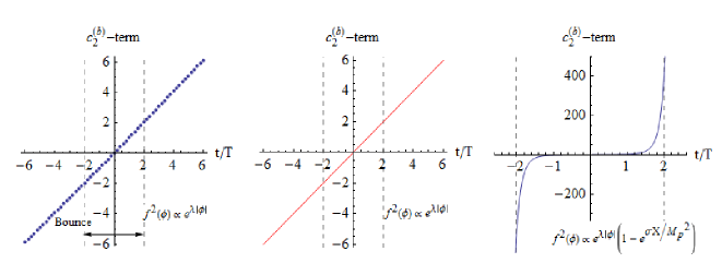
Figure 3: Left panel: growing modes solved numerically. Center panel: the linear approximation for $f^{2}(\phi)\propto e^{\lambda|\phi|}$. The plot on the right corresponds to the model $f^{2}(\phi,\dot{\phi})\propto e^{\lambda|\phi|}\dot{\phi}^{2}/M_{p}^{2}$

In the previous analysis we saw that the model had a problem just at the bounce point that was avoided with a smoothed approximation. Yet, it may be interesting to consider another ansatz for the coupling function, that depends with $\phi$ and $X$. We tried,

$$f^{2}(\phi,X)=e^{\lambda(|\phi|-\phi_{\mathrm{end}})}\left(1-e^{\sigma\frac{X}{M_{p}^{2}}}\right),$$ (77)

with $0<\sigma<1$. For the present scenario we are considering, the value of the scalar field vanishes during the bounce $\phi_{b}=0$. While on the other hand, the value of its derivative increases as high as $\dot{\phi}\approx 0.1M_{p}$. This means that during the bounce we could approximate the previous expression as $f^{2}(\phi,X)\approx e^{\lambda(|\phi|-\phi_{\mathrm{end}})}\sigma\frac{\dot{\phi}^{2}}{2M_{p}^{2}}$. Again, by combining this with the approximate analytical expressions during the bounce of the scale factor(72), the time derivative of the scalar field (73) and the general expression of the coupling function (9), we obtain

$$\eta(y)=(T^{2}\Upsilon-4)y+\lambda T\dot{\phi}_{b}e^{-y^{2}}\frac{|\phi|}{\phi}.$$ (78)

A new $-4y$ term manifests. As we already stated, the last $e^{-y^{2}}$ term is negligible in the long wave length regime, while $T^{2}\Upsilon\approx TH_{b+}\left[\frac{1}{2}\ln\left(\frac{9\beta H^{2}_{b+}}{(g_{0}-1)M_{p}^{2}}\right)\right]^{-1/2}\approx TH_{b+}/2$ for the set of parameters (III.1) in Bran1206 . Thus, one obtains that $\eta(y)\approx-4y$. Which we can easily solve in terms of the imaginary error function $\mathrm{Erfi}(\sqrt{2}y)$. This is plotted on the graphic on the right in fig.(3). One can see that during the bounce this mode is amplified several orders of magnitude. Indeed, for $-2<y<2$ one obtains an amplification of almost ${\cal O}(10^{3})$. Although, we shall leave the analysis of such a possibility for future work, one can preview that backreaction problems may rise for a longer bounce period, or if the relative electromagnetic energy density $\Omega_{B}$ had grown to levels of about ${\cal O}(10^{-6})$ at the end of the ekpyrotic phase.

III.2.4 Modes through the fast-roll: $t_{\mathrm{b}+}<t<t_{\mathrm{end}}$

After the bounce finishes the universe enters a period of expansion dominated by kinetic energy of the scalar field. In this stage the equation of state is $w=1$, so it is easy to find the solution for the electromagnetic modes from the general expression (13).

$$u_{k}^{(\mathrm{f})}=c_{1}^{(\mathrm{f})}+c_{2}^{(\mathrm{f})}\left(\frac{a}{a_{\star}}\right)^{r^{(\mathrm{f})}},\hskip 28.45274ptr^{(\mathrm{f})}=-2n^{(\mathrm{f})}+2$$ (79)

As before, we have a parameter $\gamma^{(\mathrm{f})}$ given by (18) using $w=1$, then

$$\gamma^{(\mathrm{f})}=\frac{n^{(\mathrm{f})}}{2}.$$ (80)

From eq. (69) we can relate $n^{(\mathrm{f})}$ with $n^{(\mathrm{ek})}$; by using $q_{\mathrm{fast}}=1/3$ one obtains the fast-roll phase equation of state $w_{\mathrm{fast}}=1$, so

$$n^{(\mathrm{f})}=\sqrt{3q_{\mathrm{ek}}}n^{(ek)}.$$ (81)

Given that $q_{\mathrm{ek}}<1/3$ we obtain $|n^{(\mathrm{f})}|<|n^{(\mathrm{ek})}|$. Thus, as expected, we will have weak coupling in the fast-roll expanding phase $n^{\mathrm{(f)}}<0$ and no backreaction from electric fields $\gamma^{\mathrm{(f)}}<0$.

III.3 Matching conditions

In the present nonsingular bouncing model we have two time surfaces where to match the perturbations originated during the ekpyrotic phase. The first is before the bounce and after the ekpyrotic phase, $t=t_{\mathrm{b}-}$, and the second is between the bounce and the fast-roll phase, $t=t_{\mathrm{b}+}$. The functions $u_{k}$ and $\dot{u}_{k}$ should be continuous across the matching surfaces. Thus, we have four matching conditions, two at each surface, and six constants $c_{1}^{(\mathrm{ek})},c_{2}^{(\mathrm{ek})},c_{1}^{(\mathrm{b})},c_{2}^{(\mathrm{b})},c_{1}^{(\mathrm{f})}$ and $c_{2}^{(\mathrm{f})}$. Furthermore, as $c_{1}^{(\mathrm{ek})}$ and $c_{2}^{(\mathrm{ek})}$ are determined by the initial conditions, the system is completely determined. In fact, to find the amplitude of electromagnetic fields given by the model, we are only interested in how the constants $c_{1}^{(\mathrm{f})},c_{2}^{(\mathrm{f})}$ relate to $c_{1}^{(\mathrm{ek})},c_{2}^{(\mathrm{ek})}$. Using the solutions for ekpyrosis (66), the bounce phase (76) and the fast-roll period (79), it is straight forward to find

$$\left(\begin{array}[]{c}c_{1}^{(\mathrm{f})}\\ c_{2}^{(\mathrm{f})}\\ \end{array}\right)=\left(\begin{array}[]{cc}m_{11}&m_{12}\\ m_{21}&m_{22}\\ \end{array}\right)\left(\begin{array}[]{c}c_{1}^{(\mathrm{ek})}\\ c_{2}^{(\mathrm{ek})}\\ \end{array}\right),$$ (82)

with

$$\left(\begin{array}[]{cc}m_{11}&m_{12}\\ m_{21}&m_{22}\\ \end{array}\right)\simeq\left(\begin{array}[]{cc}1&1+r^{(\mathrm{ek})}H_{\mathrm{b}-}(t_{\mathrm{b}+}-t_{\mathrm{b}-})-\frac{r^{(\mathrm{ek})}H_{\mathrm{b}-}}{r^{(\mathrm{f})}H_{\mathrm{b}+}}\\ {\cal O}(k^{2})&\frac{r^{(\mathrm{ek})}H_{\mathrm{b}-}}{r^{(\mathrm{f})}H_{\mathrm{b}+}}\\ \end{array}\right),$$ (83)

where we have used that $t_{\mathrm{b}-}/t_{\mathrm{b}+}\approx H_{\mathrm{b}+}/H_{\mathrm{b}-}$. Then, we can write the quadratic amplitude,

$$|u_{k}^{(\mathrm{f})}|^{2}\simeq|c_{1}^{(\mathrm{ek})}|^{2}+|c_{2}^{(\mathrm{ek})}|^{2}\left[m_{12}^{2}+2m_{12}m_{22}\left(\frac{a}{a_{\mathrm{b}+}}\right)^{r^{(\mathrm{f})}}+m_{22}^{2}\left(\frac{a}{a_{\mathrm{b}+}}\right)^{2r^{(\mathrm{f})}}\right].$$ (84)

III.4 Evolution of seed magnetic fields

Here we will evolve the amplitude of magnetic fields that reach the reheating period. For simplicity we are assuming that the universe reheats instantaneously to the radiation era. Consider the magnetic cosmological parameter today

$$\Omega^{0}_{B}(k)\equiv\frac{\rho_{B}(t=t_{0},k)}{\rho_{\mathrm{cri}}},$$ (85)

defined at a certain scale $L=2\pi/k$. After the $\phi$ field disappears the coupling function should stay around $f_{\mathrm{end}}\gtrsim 1$, the universe enters the radiation dominated period and the energy density of magnetic fields evolve as a Maxwell field with $a^{-4}$. Ignoring any type of subsequent amplification mechanisms until the galaxy formation time, we may write

$$\small{\rho_{B}(t=t_{0},k)=\frac{d\rho_{B}}{d\ln k}(t=t_{\mathrm{end}},k)\left(\frac{a_{\mathrm{end}}}{a_{0}}\right)^{4}},$$ (86)

using the quadratic expression (84) in eq. (31) with the constants inherited from the ekpyrotic phase (25) we obtain the leading spectral contribution

$$\Omega^{0}_{B}(k)=\frac{4}{3\pi}|b_{(\gamma^{(\mathrm{ek})})}|^{2}\left(\frac{q}{1-q}\right)^{2\gamma^{(\mathrm{ek})}}\frac{H_{\mathrm{end}}^{2}}{m_{pl}^{2}}\left(\frac{H_{0}}{H_{\mathrm{end}}}\right)^{2+2\gamma^{(\mathrm{ek})}}\left(\frac{a_{0}}{a_{\mathrm{end}}}\right)^{2\gamma^{(\mathrm{ek})}}\left(\frac{k}{a_{0}H_{0}}\right)^{2\gamma^{(\mathrm{ek})}+4}.$$ (87)

To continue we need an expression for $(a_{0}/a_{\mathrm{end}})$, and thus, one needs to specify details of the reheating period. This period is at least described by the initial energy scale $\rho_{\mathrm{end}}$, the reheating temperature $T_{\mathrm{reh}}$ and the equation of state $w_{\mathrm{reh}}$. In fact, all this information can be simplified in a single parameter $R_{\mathrm{rad}}$ or $R$ described in Martin07 .

$$\frac{a_{0}}{a_{\mathrm{end}}}=\frac{1}{R}\left(\frac{\rho^{0}_{\mathrm{rad}}}{M_{p}^{4}}\right)^{-\frac{1}{4}}\left(\frac{\rho_{\mathrm{end}}}{M_{p}^{4}}\right)^{\frac{1}{2}}$$ (88)

where $\rho_{\mathrm{rad}}^{0}=\Omega^{0}_{\mathrm{rad}}\rho^{0}_{\mathrm{cri}}$. A complete treatment would involve a study of the parameter space for different models. However, we shall keep with the simplified assumption that the reheating is instantaneous. In such a case, we obtain $R=\rho_{\mathrm{end}}^{1/4}/M_{p}$, which implies that $a_{0}/a_{\mathrm{end}}=(\rho_{\mathrm{end}}/\rho^{0}_{\mathrm{rad}})^{1/4}$. Then,

$$\Omega_{B}^{0}(k)=\frac{4}{3\pi}|b_{(\gamma^{(\mathrm{ek})})}|^{2}\left(\frac{q}{1-q}\right)^{2\gamma^{(\mathrm{ek})}}{(\Omega^{0}_{\mathrm{rad}})}^{-\frac{\gamma^{(\mathrm{ek})}}{2}}\left(\frac{H_{0}}{H_{\mathrm{end}}}\right)^{2+\gamma^{(\mathrm{ek})}}\frac{H_{\mathrm{end}}^{2}}{m_{pl}^{2}}\left(\frac{k}{a_{0}H_{0}}\right)^{2\gamma^{(\mathrm{ek})}+4}.$$ (89)

Furthermore, the actual magnetic energy density is $\rho^{0}_{B}=B_{0}^{2}/2$, then we obtain an amplitude of magnetic fields

$$\frac{B_{0}}{m_{pl}^{2}}=\frac{|b_{(\gamma^{(\mathrm{ek})})}|}{\pi}\left(\frac{q}{1-q}\right)^{\gamma^{(\mathrm{ek})}}{(\Omega^{0}_{\mathrm{rad}})}^{-\frac{\gamma^{(\mathrm{ek})}}{4}}\left(\frac{H_{0}}{m_{pl}}\right)^{1+\frac{\gamma^{(\mathrm{ek})}}{2}}\left(\frac{H_{\mathrm{b}+}}{m_{pl}}\right)^{-\frac{\gamma^{(\mathrm{ek})}}{2}}e^{-\frac{3\gamma^{(\mathrm{ek})}N_{\mathrm{f}}}{4}}\left(\frac{k}{a_{0}H_{0}}\right)^{\gamma^{(\mathrm{ek})}+2}$$ (90)

where we used that $H_{\mathrm{end}}=H_{\mathrm{b}+}e^{\frac{3}{2}N_{\mathrm{f}}}$. We may express the magnetic fields in gauss through $1m_{pl}^{2}=7.64\times 10^{57}\mathrm{G}$. The measured actual Hubble parameter is close to $H_{0}=70\mathrm{km}/s\mathrm{Mpc}^{-1}=1.23\times 10^{-61}m_{pl}$Planck13cosmoparam , and the radiation ratio $\Omega^{0}_{\mathrm{rad}}=3.53\times 10^{-5}$ reviewparticle12 . Considering these, we arrive at

$$\left(\frac{B_{0}}{\mathrm{gauss}}\right)\simeq\frac{7.64\times 10^{57}(1.23\times 10^{-61})^{2+\frac{\gamma^{(\mathrm{ek})}}{2}}}{(3.53\times 10^{-5})^{\frac{\gamma^{(\mathrm{ek})}}{4}}} \frac{|b_{(\gamma^{(\mathrm{ek})})}|}{\pi}\left(\frac{q}{1-q}\right)^{\gamma^{(\mathrm{ek})}}e^{-\frac{3\gamma^{(\mathrm{ek})}N_{\mathrm{f}}}{4}}$$ (91)

$$\left(\frac{H_{\mathrm{b}+}}{m_{pl}}\right)^{-\frac{\gamma^{(\mathrm{ek})}}{2}}\left(\frac{2.7\times 10^{4}\mathrm{Mpc}}{L}\right)^{\gamma^{(\mathrm{ek})}+2},$$

an expression for actual magnetic fields at scales $L$ measured in Mpc and produced during an ekpyrotic contracting phase with equation of state $w_{\mathrm{ek}}=-1+2/3q>1$. In deriving it, we have made several assumptions. These assumptions involve the particular background evolution of the scalar field that drive the ekpyrotic phase, the bouncing, and the final fast-roll phase. We also considered an instantaneous reheating and, furthermore, we supposed that the magnetic fields are not amplified (nor consumed) by any other mechanism during the universe evolution until galaxy formation.

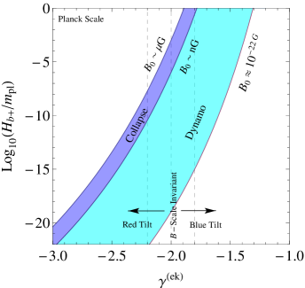
Figure 4: $\mathrm{Log}H_{b+}$ vs. $\gamma^{\mathrm{(ek)}}$ from expression (91) for $B_{0}$. We included the magnetic fields produced at $L=1Mpc$. The blue belt corresponds to the interval between $B_{0}=10^{-6}G$ and $10^{-9}G$, that account for compression of B-field lines by the collapse of the protogalaxy. The cyan belt corresponds to the dynamo mechanism needed levels up to $10^{-22}G$.

The B-spectrum it is given by the value of $\gamma^{(\mathrm{ek})}$ at the ekpyrotic phase. Its amplitude depends also on the values of the equation of state during that period through the value of $q$ and of the energy scale $H_{\mathrm{end}}$ at the onset of the reheating period. In Fig.4 we use this expression (91) to identify the regions where interesting magnetic fields maybe produced by this mechanism. We included magnetic fields between microgauss, corresponding to the actual observations on galactic scales and nanogauss, the last needed if amplification is only done by the collapsing protogalaxy. Besides, nanogauss fields correspond to upper limits inferred by Planck constraints on non-Gaussianity Plancknongauss from the bispectrum bispectrum and recently from the trispectrum trispectrum . The cyan belt corresponds to the dynamo needs for amplifying primordial magnetic fields of up to $10^{-16}\mu$G to $\mu G$ levels.

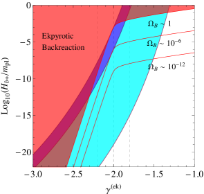
Figure 5: $\mathrm{Log}H_{b+}$ vs. $\gamma^{\mathrm{(ek)}}$, with backreaction levels during ekpyrosis of $N_{\mathrm{ek}}=75$ by using eq.(39). The red region is forbidden since there $\Omega_{B}>1$. Red lines correspond to allowed levels of backreaction $\Omega_{B}=10^{-6}$ and $\Omega_{B}=10^{-12}$. We also included the magnetic fields produced at $\sim 1Mpc$ as in fig. (4). Here, we considered that fast-roll is very short $N_{\mathrm{f}}\approx 0$ and $q=0.1$.

On Fig.5 we included the backreaction constraints from a period of contraction using Eq.(39). Though we used the value $q=0.1$, that corresponds to an ekpyrotic phase with $w\approx 5.67$, one may go for values of radiation or matter-dominated contractions without significant variations. Also, in the present model we have $H_{b+}\approx 10^{-4}m_{\mathrm{pl}}$, thus one obtains strong magnetic fields $\gtrsim 10^{-3}\mu$G if the B-spectrum is almost scale invariant $n_{B}\approx 0$. But, also for $B_{\mathrm{1Mpc}}$-fields with blue tilt up to $n_{B}=1$, one can get strengths $\sim 10^{-16}\mu$G at safe levels of backreaction $\Omega_{B}\approx 10^{-6}$.

Another interesting feature is that apparently one can relax the scale of the bouncing up to about $H_{b+}\approx 10^{-15}\sim 10^{-20}m_{\mathrm{pl}}$, keeping a low blue tilt $n_{B}=0\sim 0.4$, and still obtain interesting magnetic fields.

We note, however, that in these last calculations we ignored a durable fast-roll phase given that we used $N_{\mathrm{f}}=0$.

III.5 Red-tilt and B-instability

Initially the background model should cast for the solution of the cosmological problems of the Big-Bang. In particular, the flatness problem is solved if $aH$ grows at least $60$ e-folds in inflationary setups. However, in general, bouncing cosmologies address the flatness problem naturally, given that during the contracting phase curvature relative energy $\Omega_{k}$ decays with respect to almost every component in the universe (except, of course, a cosmological constant). Indeed, we checked that if the ekpyrotic phase is rather short, $N_{\mathrm{ek}}\lesssim 30$, the constraints on the red-tilted spectrum are significatively relaxed.

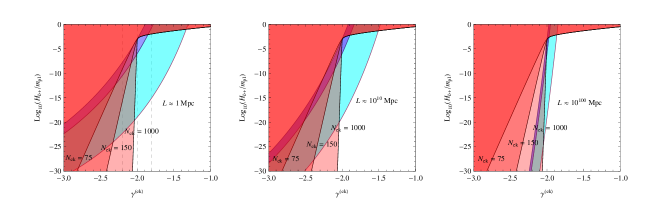
Figure 6: Regions of $\mathrm{Log}H_{b+}$ vs. $\gamma^{\mathrm{(ek)}}$ for backreaction ($\Omega_{B}\geqslant 1$) during different lasting periods of ekpyrosis, $N_{\mathrm{ek}}=75,150,1000$ (red shaded regions), and for actual magnetic fields $B_{0}$ with lengths of coherence, from left to right, $L=1,10^{10}\mathrm{and}10^{100}$Mpc.

To proceed, we would like to test how the system is sensible to develop instabilities for larger values of $N_{\mathrm{ek}}$. In Fig.6 we sketched how backreaction grows for different values of $N_{\mathrm{ek}}$. We identify that the effect is rather weak, and are needed large numbers of e-folds, $N_{\mathrm{ek}}\approx 1000$ to practically exclude the red tilted B-spectrum of magnetic fields. While the blue tilted region remains totally unharmed. We also showed the qualitative behavior of the amplitude of magnetic fields in the strengths of interest, for collapse of the protogalactic cloud: $\mu$G to $n$G (blue belt) and dynamo mechanism: $n$G to $10^{-22}$G (cyan belt), when we vary their scales of coherence $L$. We included extremely large values, in the second and third panels ($L=10^{10}\mathrm{Mpc}$ and $L=10^{100}\mathrm{Mpc}$, senseless otherwise one assumes longlasting periods $N_{ek}\gg 100$) only to illustrate the weakness of the effect. Clearly, we will be interested in the usual values about $N_{\mathrm{ek}}=75$, with B-fields at a coherence scale of $1Mpc$. Yet, variations around these values will not change significantly the general behavior.

However, we have not considered the possible instabilities during the kinetically-driven expanding phase. Nor consider how B-fields decay during this period. These will be address in the next section.

III.6 Backreaction during the fast-roll

The calculation is very similar to what we have done previously. First we need to determine the energy densities (31) and (32) using $u_{k}^{(\mathrm{f})}$. As seen before, the constants of the mode $u_{k}^{(\mathrm{f})}$ are related, through the matching conditions, to the constants of the ekpyrotic mode $u_{k}^{(\mathrm{ek})}$. These quantities were fixed by initial conditions during the ekpyrotic contracting phase, and are given by eq. (25) with the ekpyrotic values $\gamma^{(\mathrm{ek})}$ and $w=-1+2/(3q)$.

Additionally, to calculate the backreaction during this period we need to consider the interval of modes that had exited the Hubble length during the ekpyrotic contraction, and start to reenter during the fast roll phase. The initial interval to consider, it will then be given approximately by the same interval that suffered the transition from the sub-Hubble regime to the super-Hubble regime. We characterized this interval through the effective number of e-folds $N_{\mathrm{ek}}=\ln\left(\frac{a_{\mathrm{b}-}H_{\mathrm{b}-}}{a_{ek}H_{ek}}\right)$. Afterwards, as the fast-rolls period develops, comoving wavelengths reenter as the comoving Hubble length $(aH)^{-1}$ increases. This means that the effective number of e-folds $N_{\mathrm{f}}=\ln\left(\frac{a_{\mathrm{end}}H_{\mathrm{end}}}{a_{\mathrm{b}+}H_{\mathrm{b}+}}\right)$ will be negative during this phase. Clearly, if the fast-roll period is almost instantaneous, then $N_{\mathrm{f}}\approx 0$ and there are no modes reentering the Hubble sphere that can backreact on the background.

We will just keep the dominant contributions that generates instabilities during this period. We find that these are produced by the last $c_{2}^{(\mathrm{ek})}$-term proportional to $m_{22}^{2}$ in (84). The reason of this is not so difficult to understand given that during this phase the scale $a$ grows and $r^{(\mathrm{f})}=2-2n^{(\mathrm{f})}>0$. Furthermore, it is straightforward to check that electric fields also have an instability from the same term. Moreover, these two contributions are proportional and they e-fold with the same rate. Thus, we find that

$$\Omega_{B}^{(\mathrm{fast})}+\Omega_{E}^{(\mathrm{fast})} \simeq \frac{4}{3\pi}m_{22}^{2}|b_{2}(\gamma^{(\mathrm{ek})})|^{2}\left(\frac{1}{6-2\gamma^{(\mathrm{ek})}}+\frac{4r^{(\mathrm{f})2}}{4-2\gamma^{(\mathrm{ek})}}\right)\left(\frac{q}{1-q}\right)^{2-2\gamma^{(\mathrm{ek})}}\times$$ (92)

$$\frac{H^{2}_{\mathrm{b}+}}{m_{pl}^{2}}e^{[3+2(\gamma^{(\mathrm{f})}-\gamma^{(\mathrm{ek})})]N_{\mathrm{f}}}.$$

These are the only contributions that can grow during the fast-roll. The others just decay with different rates and are negligible.

It is found that $\gamma^{(\mathrm{f})}<\gamma^{(\mathrm{ek})}<0$, and noticing that for $q_{\mathrm{ek}}=1/3$ one gets $\gamma^{(\mathrm{ek})}=\gamma^{(\mathrm{f})}$, then the exponential rate is restricted to $3+2(\gamma^{(\mathrm{f})}-\gamma^{(\mathrm{ek})})<3$. We see that still there may be stability for this components as long as this rate keeps positive (one should remind that $N_{\mathrm{f}}<0$). This depends strongly on the parameter $q$ of the ekpyrotic phase, and more stability is obtained as close as $q=1/3$ we are. In another way, for sufficiently steep ekpyrotic potentials, strong instabilities may arise in a durable kinetic stiff dominated expanding phase of the scalar field. Thus, care should be taken for models where $q\ll 1$, because they are susceptible to develop $f^{2}(\phi)F^{2}$- instabilities.

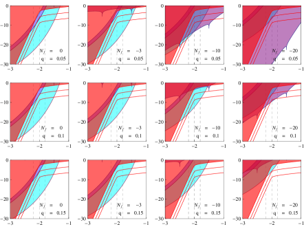
Figure 7: The scale of the bounce $Log_{10}(H_{\mathrm{b}+}/m_{pl})$ vs. the parameter $\gamma^{(\mathrm{ek})}$. In rows, from top to bottom, we listed $q=0.05,0.1$ and $0.15$. In columns, we have from left to right,the duration of the kinetic period $N_{f}=0,-3,-10$ and $-20$. The red sector corresponds to $\Omega^{(\mathrm{ek})}_{EM}>1$, backreaction produced during a $N_{\mathrm{ek}}=75$ ekpyrotic contraction phase. The purple sector corresponds to $\Omega^{(\mathrm{fast})}_{EM}>1$, backreaction during the fast-roll expansion. We included the magnetic fields produced at $\sim 1Mpc$. The blue belt corresponds to $B\sim 10^{-6}G$ to $10^{-9}G$.

III.7 Magnetic fields without backreaction

In previous sections we quantified the backreaction levels of magnetogenesis that operate during an ekpyrotic phase [see eq.(39)] and during the fast-roll phase [see eq.(92)]. We argued before that backreaction during the contracting phase is not so sensible to the value of $q$, as long as $w>-1/3$. However, this is not the case for the expanding fast-roll phase. As one may check in Fig.(7), the purple region corresponds to forbidden regions of backreaction that originate during the fast-roll phase. The values used in the present model correspond to the middle row, where $q=0.1$. In this case backreaction excludes any magnetic fields whether $(aH)$ e-folds almost $N_{\mathrm{f}}=-20$. Instead, for $N_{\mathrm{f}}=-10$ still a large window of parameters allows magnetogenesis. In particular, for $N_{\mathrm{f}}=-3$ and almost scale invariant B-fields one obtains nanogauss strengths for $H_{b+}\approx 10^{-4}\sim 10^{-5}$. Yet, the situation changes drastically when we go for lower values of $q$. For example, for $q=0.05$ (first row in fig.(7)) or $w\simeq 12.3$, we find that for $N_{\mathrm{f}}=-10$, backreaction has practically excluded all possible parameters. In contrast, when $q=0.15$ (last row) which corresponds with $w\simeq 3.4$, it is safe from backreaction. This behavior is related to the differences between the equations of state during the contracting and expanding phases. In this sense, we find that backreaction is enhanced when this differences are stronger. In our case, when $q$ becomes much smaller that $1/3$. From the potential point of view, a lower value of $q$ corresponds to steeper potentials, while during the fast-roll phase it is assumed that the potential is much more flat. In turn, this would mean that the system is unstable against strong differences in the slopes of the potential between the downward and the upward branch.

In this sense we find that in scenarios with an ekpyrotic contraction and a fast-roll-stiff period, magnetogenesis is possible as long as $q\lesssim 1/3$. It is remarkably that in Bran1206 they found that the spectral index of thermally seeded scalar fluctuations is $n_{s}=4q/(1-q)$. Thus, one obtains the slightly red spectrum for very close values below $q=1/5$. In this case stability is guaranteed.

In a more general framework we may think that instabilities appear related to the asymmetries of the potential $V(\phi)$. Or in another way, symmetric potentials are stable.

IV Conclusions

In the present work we have analyzed the primordial magnetogenesis issue from the coupling of a scalar field to a $U(1)$ gauge field. Particularly we focused our study in the $f^{2}(\phi)F^{2}$-class models.

The first part of the paper was devoted to analyze the known problems of backreaction and strong coupling that plague this scenarios in the inflationary case. As a result we found that, in general, inflation cannot support magnetogenesis without going to the strong coupling regime. This was realized since we found that when $w<-1/3$ (required by any inflationary model), one obtains different signs of $\gamma$ and $n$. Indeed, we showed that for the values $\gamma<0$, B-fields dominate the spectrum, thus we speak of magnetogenesis. On the other side, $\gamma>0$ makes E-fields lead the spectrum and electrogenesis is achieved. Furthermore, the strong coupled regime is for $n>0$. In this sense, in inflationary scenarios one should keep $n<0$ which automatically yields $\gamma>0$. This means looking for B-fields in a place where E-fields dominate and strong instabilities from backreaction arise.

On the other side, both problems can be solved whether we have an early cosmological period with $w>-1/3$ (meaning $\gamma$ and $n$ of the same sign), and with the coupling $f(\phi)$. Such candidates belong to bouncing cosmologies, that have a period of contraction, which in order to generate large scale fluctuations, need to have a shrinking Hubble sphere during contraction. Contrary to an expanding inflation cosmology, this is achieved when $w>-1/3$.

Consequently, the second part of our work consisted in applying this arguments to a specific bouncing cosmology scenario. We chose a model where the bouncing is non-singular Bran1206 , that makes it much easier to follow the modes through the different phases. Here, the primordial spectrum of matter inhomogeneities is addressed by considering an initial matter-dominated phase ($w\simeq 0$) that evolves through an ekpyrotic period of contraction that washes out anisotropies present at the start Bran1301 . All the work is done by a background scalar field in an ekpyrotic-like potential. After, when the scalar field gets close to the minimum of the potential, a brief ghost condensate phase turns on, during which the universe bounces. Finally, the scalar field enters a flatter branch of the potential, dominated by kinetic energy, yielding a stiff-like period of expansion, where the scalar field decays with respect to the other components of the universe regarding the initial conditions for reheating and the standard Big-Bang.

What we done was to introduce the $f^{2}(\phi)F^{2}$ theory in the background bouncing dynamics. Though the scenario starts from an initial matter-dominated phase, we decided to describe only the electromagnetic fields generated by vacuum fluctuations during the ekpyrotic phase. The reason for this was to keep as simple and general as possible, given that ekpyrotic contracting periods before the bounce are commonly needed conditions to evade the instabilities of anisotropies, and belong to many bouncing universe models. However, we suppose that the extension to consider other previous phases to ekpyrosis should not in general be so problematic as long as $-1/3<w<1$. Next we needed to choose a specific coupling function $f(\phi)$ of the $e^{\lambda\phi}$ type [see eq. (68)]. With it we obtained the relation (69) between the coupling parameter $n$ and the equation of state $w=-1+2/(3q)$. Finally, we could define the solutions for the modes in the long wavelength regime for ekpyrosis, bounce, and fast-roll phases.
At the same time we computed the relative energy density of the electromagnetic field during ekpyrosis and the fast-roll expanding phase.

This was necessary to follow the levels of backreaction of the perturbations during its evolution. On the other side, instabilities during the bounce period are negligible. This should be clear from eq. (76), where the solution for the modes is practically linear and the duration of the bounce is very short. However, this could turn to be a very particular case. Indeed, as we showed in another example, one can obtain large amplification even during short bouncing phases.

When analyzing backreaction we first found that the duration of the ekpyrotic contracting phase, characterized in the effective number of e-folds of $a|H|$, can at least exclude the red tilted spectrum $(\gamma^{\mathrm{(ek)}}<-2)$ if it goes for more than about $\sim 1000$ e-folds. But it left the blue tilted region of the parameters unconstrained [see fig.6]. Indeed, such a behavior seems compatible with cyclic scenarios cyclic .

Moreover, a newly interesting feature is that the fast-roll expanding period could develop strong instabilities of backreaction if $q\ll 1/3$. This would mean that strong ekpyrotic periods could turn to be unstable for such theories. Indeed, a related study involving $p-$forms was previously done in Steinhardt0312 . On the other side, as in the present bouncing model, weaker ekpyrotic phases favor a safer magnetogenesis.

From a physical point of view, a stronger ekpyrotic phase can be identified with a steeper potential for the scalar field. In this sense, as we noticed when considering the backreaction during the stiff fast-roll phase, instabilities appear for steeper potentials. This means that stability is obtained for rather symmetric potentials.

Finally, to complete our work we estimated present amplitude of magnetic fields generated from this early epochs. As expected a broad range of parameters can account for the needed strengths of B-fields. This should be identified with the fact that contracting cosmologies allowed us to work with the magnetogenesis branch $\gamma<0$. As was previously observed, for this case B-fields dominate the spectrum of the electromagnetic fields.

Finally we expect that contracting universes dominated by matter or radiation, previous to the ekpyrotic washing of anisotropies, can also account for amplification of vacuum fluctuations of the gauge field (as long as the coupling $f(\phi)$ exists). Indeed, given that the Hubble sphere shrinks when $\dot{a}<0$ and $w>-1/3$, an interval of wavelengths suffers the ’freezing’ on cosmological scales, go through the ekpyrotic phase, the bounce and reenter on late times. In such a case, one immediately sees [cf. eq.(69)] that the coupling parameter remains in the weak coupling regime through all the evolution. Apart, a bouncing phase can also originate from pure quantum cosmological effects. They also provide a natural framework in which a dust-dominated contraction is easily implemented to yield a scale-invariant spectrum of perturbation PintoNeto .

The recent BICEP2 experiment data release BICEP2 detected cosmological gravitational waves over $5\sigma$, from measurement of the B-mode polarization of the CMB. The tensor-to-scalar ratio found is $r=0.2^{+0.07}_{-0.05}$. In this sense, the original ekpyrotic and cyclic universe scenarios, that predict very low gravitational wave production, are strongly constrained.

However, we would like to remark that in the present paper we find, as a general result, that early contracting cosmological phases with $w>-1/3$ support magnetic field generation safe from the backreaction/strong-coupling problem. Indeed, it has been argued that combining BICEP2 and POLARBEAR POLARBEAR polarization data, a preference for blue tensor spectrum is obtained Xue1403 . In particular, we considered a bouncing universe example that belongs to the matter-bounce scenarios. In this realization, tensor perturbations are nearly scale-invariant but the amplitudes too high. Yet, from the two-field picture Bran1305 the tensor modes become a tunable parameter. Thus, it should be further studied if this background model fits the observations. Moreover, we expect that bouncing models that can fit the observed tensor-to-scalar ratio will also be able to support magnetogenesis.

References

- (1) U. Klein, R. Wielebinski and H.W. Morsi, Astron. & Astrophys. 190 (1988) 41. K. Kim et al., Nature 341 (1989) 720. P.P. Kronberg, Reports on Progress in Physics 57 (1994) 325. J. Han and R. Wielebinski, Chin. J. Astron. Astrophys. 2 (2002) 293, [arXiv:astro-ph/0209090]. C.L. Carilli and G.B. Taylor, Ann. Rev. Astron. & Astrophys. 40 (2002) 319, [arXiv:astroph/0110655]. J.P. Vall ee, New Astron. Rev. 48 (2004) 763. R. Beck et al., Astron. & Astrophys. 444 (2005) 739, [arXiv:astro-ph/0508485].
- (2) Shin’ichiro Ando, Alexander Kusenko, Astrophys.J. 722 (2010) L39, e-Print: arXiv:1005.1924 [astro-ph.HE]. Warren Essey, Shin’ichiro Ando, Alexander Kusenko, Astropart.Phys. 35 (2011) 135-139, e-Print: arXiv:1012.5313 [astro-ph.HE]
- (3) H.K. Moffatt, Magnetic Field Generation in Electrically Conducting Fluids (Cambridge University Press, 1978). E.N. Parker, Cosmical Magnetic Fields (Oxford: Clarendon Press, 1979). I.B. Zeldovich, A.A. Ruzmaikin and D.D. Sokolov, Magnetic Fields in Astrophysics (New York: Gordon and Breach, 1983). R.M. Kulsrud and S.W. Anderson, Astrophys. J. 396 (1992) 606.94. F. Krause, in The Cosmic Dynamo, edited by . F. Krause, K. H. Radler, & G. Rudiger, IAU Symposium Vol. 157, p. 487, 1993. J.L. Han et al., Astron. & Astrophys. 322 (1997) 98. A. Brandenburg and K. Subramanian, Phys. Rep. 417 (2005) 1, [arXiv:astro-ph/0405052].
- (4) Xu, Yongzhong et al. Astrophys.J. 637 (2006) 19-26 astro-ph/0509826 LA-UR-05-3143
- (5) P.P.Kronberg et al., Astrophys. J. 676 (2008) 70, [arXiv:0712.0435]. M.L. Bernet et al., Nature 454 (2008) 302, [arXiv:0807.3347]. A.M. Wolfe et al., Nature 455 (2008) 638, [arXiv:0811.2408].
- (6) Grasso, Dario et al. Phys.Rept. 348 (2001) 163-266 astro-ph/0009061 DFPD-00-TH-35. Widrow, Lawrence M., Rev.Mod.Phys.74,775-823(2002) astro-ph/0207240. Giovannini, Massimo, Int.J.Mod.Phys. D13 (2004) 391-502 CERN-TH-2003-307 astro-ph/0312614. Kandus, Alejandra et al. Phys.Rept. 505 (2011) 1-58 arXiv:1007.3891 [astro-ph.CO]. Durrer, R. and Neronov, A., ”Cosmological Magnetic Fields: Their Generation, Evolution and Observation”, e-Print: arXiv:1303.7121 [astro-ph.CO].
- (7) M.S. Turner and L.M. Widrow, Phys. Rev. D 37 (1988) 2743.
- (8) B. Ratra, Astrophys. J. 391, L1 (1992);
- (9) M. Gasperini, M. Giovannini and G. Veneziano, Phys. Rev. Lett. 75, 3796 (1995). e-Print: hep-th/9504083
- (10) L. Campanelli, P. Cea, G.L. Fogli, L. Tedesco (Bari U. & INFN, Bari) Phys.Rev. D77 (2008) 123002, e-print: arXiv:0802.2630 [astro-ph]
- (11) M., Jerome and Yokoyama, J., JCAP 0801 (2008) 025, e-Print: arXiv:0711.4307 [astro-ph]
- (12) Demozzi, V. and Mukhanov, V. and Rubinstein, H., JCAP 0908 (2009) 025, e-Print: arXiv:0907.1030 [astro-ph.CO]
- (13) M. Novello and S. E. P. Bergliaffa, Phys. Rept. 463, 127 (2008) [arXiv:0802.1634 [astro-ph]]. M. Novello and J. Salim, Phys. Rev. D20, 377 (1979).
- (14) V.A. Belinsky, I.M. Khalatnikov, E.M. Lifshitz, ”Oscillatory approach to a singular point in the relativistic cosmology”, Adv. Phys. 19 (1970) 525.
- (15) J. Khoury, B.A. Ovrut, P.J. Steinhardt, N. Turok, Phys. Rev. D 64 (2001)123522. arXiv:hep-th/0103239.
- (16) P.J. Steinhardt, N. Turok, Phys. Rev. D 65 (2002) 126003. arXiv:hep-th/0111098. P.J. Steinhardt, N. Turok, Science 296 (2002) 1436. P.J. Steinhardt, N. Turok, New Astron. Rev. 49 (2005) 43. arXiv:astro-ph/0404480.
- (17) E.I. Buchbinder, J. Khoury, B.A. Ovrut, Phys. Rev. D 76 (2007) 123503. arXiv:hep-th/0702154. E.I. Buchbinder, J. Khoury, B.A. Ovrut, JHEP 0711 (2007) 076. arXiv:0706.3903 [hep-th].
- (18) Jean-Luc Lehners, Phys.Rept. 465 (2008) 223-263. e-Print: arXiv:0806.1245 [astro-ph].
- (19) A. Nicolis, R. Rattazzi and E. Trincherini, Phys. Rev. D 79, 064036 (2009) [arXiv:0811.2197 [hep-th]]; C. Def- fayet, G. Esposito-Farese and A. Vikman, Phys. Rev. D 79, 084003 (2009) [arXiv:0901.1314 [hep-th]]; A. Nicolis, R. Rattazzi and E. Trincherini, JHEP 1005, 095 (2010) [Erratum-ibid. 1111, 128 (2011)] [arXiv:0912.4258 [hep- th]]. C. Deffayet, S. Deser and G. Esposito-Farese, Phys. Rev. D 80, 064015 (2009) [arXiv:0906.1967 [gr-qc]]; C. Def- fayet, X. Gao, D. A. Steer and G. Zahariade, Phys. Rev. D 84, 064039 (2011) [arXiv:1103.3260 [hep-th]]. F. P. Silva and K. Koyama, Phys. Rev. D 80, 121301 (2009) [arXiv:0909.4538 [astro-ph.CO]]; P. Creminelli, A. Nicolis and E. Trincherini, JCAP 1011, 021 (2010) [arXiv:1007.0027 [hep-th]]; C. Deffayet, S. Deser and G. Esposito-Farese, Phys. Rev. D 82, 061501 (2010) [arXiv:1007.5278 [gr-qc]]; C. Deffayet, O. Pujolas, I. Sawicki and A. Vikman, JCAP 1010, 026 (2010) [arXiv:1008.0048 [hep-th]]; T. Kobayashi, M. Yamaguchi and J. i. Yokoyama, Phys. Rev. Lett. 105, 231302 (2010) [arXiv:1008.0603 [hep-th]]; L. Levasseur Perreault, R. Brandenberger and A. -C. Davis, Phys. Rev. D 84, 103512 (2011) [arXiv:1105.5649 [astro-ph.CO]]; Z. G. Liu, J. Zhang and Y. S. Piao, Phys. Rev. D 84, 063508 (2011), arXiv:1105.5713 [astro-ph.CO]; T. Kobayashi, M. Yamaguchi and J. i. Yokoyama, Prog. Theor. Phys. 126, 511 (2011) [arXiv:1105.5723 [hep-th]]; J. Evslin, T. Qiu, JHEP 1111, 032 (2011) [arXiv:1106.0570 [hep- th]]; X. Gao and D. A. Steer, JCAP 1112, 019 (2011) [arXiv:1107.2642 [astro-ph.CO]]; X. Gao, T. Kobayashi, M. Yamaguchi and J. i. Yokoyama, Phys. Rev. Lett. 107, 211301 (2011) [arXiv:1108.3513 [astro-ph.CO]]; H.Wang, T. Qiu and Y. -S. Piao, Phys. Lett. B 707, 11 (2012) [arXiv:1110.1795 [hep-ph]]; A. De Felice and S. Tsu- jikawa, JCAP 1202, 007 (2012) [arXiv:1110.3878 [gr-qc]]; M. Li, T. Qiu, Y. Cai and X. Zhang, JCAP 1204, 003 (2012) [arXiv:1112.4255 [hep-th]]; X. Gao, T. Kobayashi, M. Shiraishi, M. Yamaguchi, J. i. Yokoyama and 13 S. Yokoyama, arXiv:1207.0588 [astro-ph.CO]; Z. -G. Liu and Y. -S. Piao, Phys. Lett. B 718, 734 (2013) [arXiv:1207.2568 [gr-qc]]; G. Leon and E. N. Saridakis, arXiv:1211.3088 [astro-ph.CO]. G. W. Horndeski, Int. J. Theor. Phys. 10, 363 (1974). T. Qiu, J. Evslin, Y. -F. Cai, M. Li and X. Zhang, JCAP 1110, 036 (2011) [arXiv:1108.0593 [hep-th]]. D. A. Easson, I. Sawicki and A. Vikman, JCAP 1111, 021 (2011) [arXiv:1109.1047 [hep-th]]. C. Lin, R. H. Brandenberger and L. Levasseur Perreault, JCAP 1104, 019 (2011) [arXiv:1007.2654 [hep-th]. Tirthabir Biswas, Erik Gerwick, Tomi Koivisto, Anupam Mazumdar, Phys.Rev.Lett. 108 (2012) 031101, e-Print: arXiv:1110.5249 [gr-qc]. Tirthabir Biswas, Alexey S. Koshelev, Anupam Mazumdar, Sergey Yu. Vernov, JCAP 1208 (2012) 024, e-Print: arXiv:1206.6374 [astro-ph.CO]. Tirthabir Biswas, Tomi Koivisto, Anupam Mazumdar, JCAP 1011 (2010) 008, e-Print: arXiv:1005.0590 [hep-th]. Tirthabir Biswas, Anupam Mazumdar, Warren Siegel, JCAP 0603 (2006) 009, e-Print: hep-th/0508194.
- (20) Creminelli, Paolo and Luty, Markus A. and Nicolis, Alberto and Senatore, Leonardo, JHEP 0612 (2006) 080. e-Print: hep-th/0606090.
- (21) J.M. Salim, N. Souza, Santiago E. Perez Bergliaffa, T. Prokopec, JCAP 0704 (2007) 011.e-Print: astro-ph/0612281.
- (22) Ferreira, Ricardo J.Z. and Jain, Rajeev Kumar and Sloth, Martin S., JCAP 1310 (2013) 004. e-Print: arXiv:1305.7151 [astro-ph.CO].
- (23) Cai, Yi-Fu and Easson, D. A. and Brandenberger, R., JCAP 1208 (2012) 020. e-Print: arXiv:1206.2382 [hep-th]
- (24) Robert Brandenberger, Phys.Rev. D80 (2009) 043516, e-Print: arXiv:0904.2835 [hep-th]
- (25) Cai, Yi-Fu and Brandenberger, R. and Peter, P., Class.Quant.Grav. 30 (2013) 075019 e-Print: arXiv:1301.4703 [gr-qc]
- (26) Yi-Fu Cai, Evan McDonough, Francis Duplessis, Robert Brandenberger, JCAP10(2013)024, e-Print: arXiv:1305.5259 [hep-th].
- (27) Xue, B., Garfinkle, D., Pretorius, F. and Steinhardt, P.J., Phys.Rev. D88 (2013) 083509. e-Print: arXiv:1308.3044 [gr-qc]
- (28) A. Maleknejad, M.M. Sheikh-Jabbari, J. Soda, Phys.Rept. 528 (2013) 161-261.e-Print: arXiv:1212.2921 [hep-th]. Masa-aki Watanabe, Sugumi Kanno, Jiro Soda Phys.Rev.Lett. 102 (2009) 191302.
- (29) J. Tate Deskins, John T. Giblin, Robert R. Caldwell, Phys.Rev. D88 (2013) 063530, e-Print: arXiv:1305.7226 [astro-ph.CO].
- (30) R. R. Caldwell, L. Motta, and M. Kamionkowski, Phys. Rev. D84 (2011) 123525, [arXiv:1109.4415]. L. Motta and R. R. Caldwell, Phys.Rev. D85 (2012) 103532, [arXiv:1203.1033]. N. Barnaby, R. Namba, and M. Peloso, Phys. Rev. D85 (2012) 123523, [arXiv:1202.1469]. R. K. Jain and M. S. Sloth, Phys.Rev. D86 (2012) 123528, [arXiv:1207.4187]. R. K. Jain and M. S. Sloth, JCAP 1302 (2013) 003, [arXiv:1210.3461]. M. Shiraishi, S. Saga, and S. Yokoyama, JCAP 1211 (2012) 046, [arXiv:1209.3384].
- (31) Latham A. Boyle, Paul J. Steinhardt, Neil Turok . Phys.Rev. D70 (2004) 023504. e-Print: hep-th/0403026
- (32) P. Ade et al. [Planck Collaboration] ”Cosmological parameters” (2013), e-Print: arXiv:1303.5076 [astro-ph.CO]
- (33) Beringer, J. and others, Review of Particle Physics 2012, Phys.Rev. D86 (2012) 010001
- (34) P. Ade et al. [Planck Collaboration] ”Constraints on primordial non-Gaussianity” (2013), e-Print: arXiv:1303.5084 [astro-ph.CO].
- (35) T. R. Seshadri and K. Subramanian, Phys. Rev. Lett. 103, 081303 (2009) [arXiv:0902.4066]; C. Caprini, F. Finelli, D. Paoletti and A. Riotto, JCAP 0906, 021 (2009) [arXiv:0903.1420]; P. Trivedi, K. Subramanian, and T. R. Seshadri (2010) [arXiv:1009.2724]. M. Shiraishi, D. Nitta, S. Yokoyama, K. Ichiki and K. Takahashi, Phys. Rev. D83, 123003 (2011) [arXiv:1103.4103]; P. Trivedi, T. R. Seshadri and K. Subramanian, Phys. Rev. Lett. 108, 231301 (2012) [arXiv:1111.0744]; M. Shiraishi and T. Sekiguchi, arXiv:1304.7277.
- (36) P. Trivedi, K. Subramanian and T. R. Seshadri, Phys. Rev. B89, 043523 (2014) [arXiv:1312.5308].
- (37) Joel K. Erickson, Daniel H. Wesley, Paul J. Steinhardt, Neil Turok. Phys.Rev. D69 (2004) 063514. e-Print: hep-th/0312009
- (38) J. Acacio de Barros, N. Pinto-Neto and M. A. Sagorio- Leal, Phys. Lett. A 241, 229 (1998). P. Peter, E. Pinho and N. Pinto-Neto, Phys. Rev. D 75, 023516 (2007); P. Peter and N. Pinto-Neto, Phys. Rev. D 78, 063506 (2008).
- (39) P. A. R. Ade et al. [BICEP2 Collaboration], e-Print: arXiv:1403.3985 [astro-ph.CO].
- (40) P. A. R. Ade et al. [The POLARBEAR Collaboration], arXiv:1403.2369 [astro-ph.CO].
- (41) Yi Wang, Wei Xue, e-Print: arXiv:1403.5817 [astro-ph.CO]