Polarized $\chi_{c2}$-charmonium production in antiproton-nucleus interactions

Abstract

Starting from the Feynman diagram representation of multiple scattering we consider the polarized $\chi_{c}$(1P)-charmonia production in antiproton-nucleus reactions close to the threshold ($p_{\rm lab}=5-7$ GeV/c). The rescattering and absorption of the incoming antiproton and outgoing charmonium on nucleons are taken into account, including the possibility of the elastic and nondiagonal (flavor-conserving) scattering $\chi_{cJ}N\to\chi_{cJ^{\prime}}N$, $J,J^{\prime}=0,1,2$. The elementary amplitudes of the latter processes are evaluated by expanding the physical $\chi_{c}$-states in the Clebsch-Gordan series of the $c\bar{c}$ states with fixed values of internal orbital angular momentum ($L_{z}$) and spin projections on the $\chi_{c}$ momentum axis. The total interaction cross sections of these $c\bar{c}$ states with nucleons have been calculated in previous works using the QCD factorization theorem and the nonrelativistic quarkonium model and turned out to be strongly $L_{z}$-dependent due to the transverse size difference. This directly leads to finite values of the $\chi_{c}$-nucleon nondiagonal scattering amplitudes. We show that the $\chi_{c0}N\to\chi_{c2}N$ transitions significantly influence the $\chi_{c2}$-production with helicity zero at small transverse momenta. This can serve as a signal in future experimental tests of the quark structure of $\chi_{c}$-states by the PANDA collaboration at FAIR.

I Introduction

It is well established, that in the perturbative QCD regime, $r_{t}\to 0$, the total cross section of a quarkonium state interaction with a proton scales as the square of the transverse separation $r_{t}$ between quark and antiquark, $\sigma_{\bar{q}q}(r_{t})\propto r_{t}^{2}$. This indicates that extracting the total quarkonium-nucleon cross section gives access to the transverse size of the quarkonium, although at $r_{t}>0.2-0.5$ fm the deviations from a simple proportionality become important (the energy dependence of the dipole-nucleon cross section also modifies this relation). If the relative coordinate wave function of the quarkonium is nonisotropic (P,D,…states), it is, thus, natural to expect that the cross section will depend on the quarkonium polarization.

This was first predicted in Ref. Gerland et al. (1998), where the cross sections of the charmonium- and bottomonium-nucleon interaction have been calculated on the basis of the QCD factorization theorem and the nonrelativistic quarkonium model. Indeed, for the 1P $\chi_{c}$- and $\chi_{b}$-states this resulted in a quarkonium polarization dependent total interaction cross section with a nucleon. Qualitatively similar results were obtained later in Ref. Hüfner et al. (2000), however, with somewhat different absolute values of the charmonium-nucleon cross sections.

Analyzing charmonium production in relativistic heavy-ion collisions, the authors of Ref. Gerland et al. (1998) predicted, that the survival probabilities of $\chi$ states with different polarization will, therefore, be different. This color filtering effect has been included afterwards in dynamical UrQMD simulations of heavy-ion collisions Spieles et al. (1999) to successfully describe $J/\psi$ production at SPS energies. Unfortunately, heavy-ion collisions involve too complex processes and it is difficult to use them to access the true charmonium-nucleon cross sections Vogt (1999).

Antiproton-nucleus collisions give the unique opportunity to study nuclear interactions of the slowly moving charmonium states exclusively formed in $\bar{p}p\to\Psi$ reactions inside the nuclear medium Brodsky and Mueller (1988); Farrar et al. (1990). Here, $\Psi$ stands for any charmonium state ($J/\psi,~{}\psi^{\prime},~{}\chi_{c}$…) decaying to $\bar{p}p$. In this paper we show that owing to the polarization-dependent $\chi_{c}$-nucleon cross sections the produced $\chi_{c2}$ states in near-threshold $\bar{p}$-nucleus collisions should reveal a significant polarization signal. Complementary information can be obtained in $\gamma A\to J/\psi A^{*}$ reactions at $E_{\gamma}\sim 10$ GeV which will be studied at the upgraded TJNAF facility.

We calculate the Feynman multiple scattering diagrams in the generalized eikonal approximation (GEA) Frankfurt et al. (1997); Sargsian (2001). The direct formation mechanism $\bar{p}p\to\chi_{c}$, as well the corrections due to the rescattering of incoming antiproton and outgoing charmonium states on nucleons, including the possibility of nondiagonal transitions, are taken into account. The nondiagonal transitions $\chi_{J_{1}\nu}N\to\chi_{J\nu}N$ are easily possible due to the small ($\sim 140$ MeV) mass splitting between the various $\chi_{c}$ states. We show that the nondiagonal transitions strongly enhance the polarization signal with respect to the color filtering mechanism only.

In sec. II we describe our model. Section III contains the results of the numerical calculations for the transverse momentum differential cross sections of $\chi_{c}$ production with different total angular momenta and helicities. At the end of sec. III we propose concrete signals for the future PANDA experiment at FAIR. Section IV summarizes the main results of this work. Appendix A contains the derivation of the expressions for the multiple scattering amplitudes.

II Model

In the following for brevity we denote as $\chi_{J}$ the $\chi_{cJ}$ charmonium with the total angular momentum $J$ ($J=0,1,2$). When explicitly needed, we will also use the notation $\chi_{J\nu}$ for the $\chi_{cJ}$ states with the fixed helicity $\nu$ ($\nu=-J,\ldots,J$).

Let us first consider only one- and two-step reactions. In this approximation, all possible diagrams contributing to the exclusive process ${\bar{p}}A\to\chi_{J}(A-1)^{*}$ are shown in Fig. 1. We neglect the contribution of the processes where $\bar{p}$ first excites to $\bar{N}^{*}$ and next the reaction $\bar{N}^{*}+p\to\chi_{J}$ takes place. This should be a reasonable assumption since at the beam momentum of 5.7 GeV/c the diffractive cross section $\sigma(\bar{p}p\to\bar{N}^{*}p+\mbox{c.c.})=0.13\pm 0.02$ mb Atherton et al. (1976) is two orders of magnitude smaller than the elastic $\bar{p}p$ cross section ($\simeq 15$ mb) at the same beam momentum. (Another reason is that the Dalitz plots for the $\chi_{c}\to\bar{p}p\pi^{0}$ decay reported by CLEO Onyisi et al. (2010) do not show any structures at $M_{\bar{p}\pi^{0}}^{2}\simeq 2$ GeV² or at $M_{p\pi^{0}}^{2}\simeq 2$ GeV². Hence the $\chi_{c}$ coupling to the $\bar{N}^{*}N$ (+c.c.) states is not expected to be significant.)

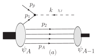
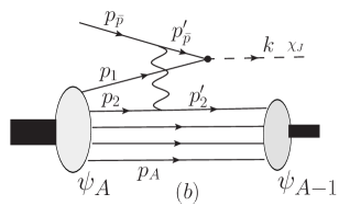
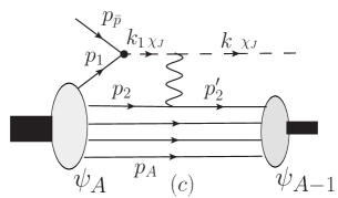
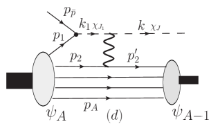
Figure 1: (a) The diagram for the production of the charmonium state $\chi_{J}$ with four-momentum $k$ in the impulse approximation. (b) The diagram taking into account elastic rescattering of the incoming antiproton on a nucleon. (c) The diagram with rescattering $\chi_{J}N_{2}\to\chi_{J}N_{2}^{\prime}$ of the initially produced $\chi_{J}$-state on a nucleon. (c) The diagram with the initial production of another state $\chi_{J_{1}}$ followed by the nondiagonal transition $\chi_{J_{1}}N_{2}\to\chi_{J}N_{2}^{\prime}$. $p_{\bar{p}}^{\prime}$, $k_{1}$ and $p_{2}^{\prime}$ are the four-momenta of the intermediate antiproton and charmonium states and of the scattered nucleon $N_{2}^{\prime}$, respectively.

The amplitudes for the processes (a),(b),(c) and (d) are, respectively

$$M^{J}(1) = \frac{M_{J;{\bar{p}}p}(\mathbf{k}-\mathbf{p}_{\bar{p}})}{\sqrt{2E_{1}}}\int d^{3}x_{1}...d^{3}x_{A}\psi^{*}_{A-1}(\mathbf{x}_{2},...,\mathbf{x}_{A})$$ (1)

$$\times \mbox{e}^{-i(\mathbf{k}-\mathbf{p}_{\bar{p}})\mathbf{x}_{1}}\psi_{A}(\mathbf{x}_{1},\mathbf{x}_{2},...,\mathbf{x}_{A})~{},$$

$$M^{J}(2,1) = \frac{1}{\sqrt{2E_{1}}2E_{2}(2\pi)^{6}}\int d^{3}x_{2}^{\prime}d^{3}x_{1}...d^{3}x_{A}\psi^{*}_{A-1}(\mathbf{x}_{2}^{\prime},\mathbf{x}_{3},...,\mathbf{x}_{A})$$ (2)

$$\times \psi_{A}(\mathbf{x}_{1},\mathbf{x}_{2},...,\mathbf{x}_{A})\int d^{3}p_{2}^{\prime}d^{3}p_{1}d^{3}p_{2}\mbox{e}^{i\mathbf{p}_{2}^{\prime}\mathbf{x}_{2}^{\prime}-i\mathbf{p}_{1}\mathbf{x}_{1}-i\mathbf{p}_{2}\mathbf{x}_{2}}$$

$$\times \delta^{(3)}(\mathbf{p}_{\bar{p}}+\mathbf{q}_{2}+\mathbf{p}_{1}-\mathbf{k})\frac{M_{J;{\bar{p}}p}(\mathbf{k}-\mathbf{p}_{\bar{p}}^{\prime})M_{\bar{p}N}(\mathbf{q}_{2})}{D_{\bar{p}}(p_{\bar{p}}^{\prime})}~{},$$

$$M^{J}(1,2) = \frac{1}{\sqrt{2E_{1}}2E_{2}(2\pi)^{6}}\int d^{3}x_{2}^{\prime}d^{3}x_{1}...d^{3}x_{A}\psi^{*}_{A-1}(\mathbf{x}_{2}^{\prime},\mathbf{x}_{3},...,\mathbf{x}_{A})$$ (3)

$$\times \psi_{A}(\mathbf{x}_{1},\mathbf{x}_{2},...,\mathbf{x}_{A})\int d^{3}p_{2}^{\prime}d^{3}p_{1}d^{3}p_{2}\mbox{e}^{i\mathbf{p}_{2}^{\prime}\mathbf{x}_{2}^{\prime}-i\mathbf{p}_{1}\mathbf{x}_{1}-i\mathbf{p}_{2}\mathbf{x}_{2}}$$

$$\times \delta^{(3)}(\mathbf{p}_{\bar{p}}+\mathbf{p}_{1}+\mathbf{q}_{2}-\mathbf{k})\frac{M_{JN}(\mathbf{q}_{2})M_{J;{\bar{p}}p}(\mathbf{k}_{1}-\mathbf{p}_{\bar{p}})}{D_{J}(k_{1})}~{},$$

$$M^{J_{1}J}(1,2) = \frac{1}{\sqrt{2E_{1}}2E_{2}(2\pi)^{6}}\int d^{3}x_{2}^{\prime}d^{3}x_{1}...d^{3}x_{A}\psi^{*}_{A-1}(\mathbf{x}_{2}^{\prime},\mathbf{x}_{3},...,\mathbf{x}_{A})$$ (4)

$$\times \psi_{A}(\mathbf{x}_{1},\mathbf{x}_{2},...,\mathbf{x}_{A})\int d^{3}p_{2}^{\prime}d^{3}p_{1}d^{3}p_{2}\mbox{e}^{i\mathbf{p}_{2}^{\prime}\mathbf{x}_{2}^{\prime}-i\mathbf{p}_{1}\mathbf{x}_{1}-i\mathbf{p}_{2}\mathbf{x}_{2}}$$

$$\times \delta^{(3)}(\mathbf{p}_{\bar{p}}+\mathbf{p}_{1}+\mathbf{q}_{2}-\mathbf{k})\frac{M_{JN^{\prime};J_{1}N}(\mathbf{q}_{2})M_{J_{1};{\bar{p}}p}(\mathbf{k}_{1}-\mathbf{p}_{\bar{p}})}{D_{J_{1}}(k_{1})}~{},$$

where $q_{2}=p_{2}-p_{2}^{\prime}$ is the four-momentum transfer from the nucleon-scatterer. Here $E_{1}$ and $E_{2}$ are the single-particle energies of the involved nucleon states $N_{1}$ (proton) and $N_{2}$, neglecting the energy difference between the scattered nucleon $N_{2}^{\prime}$ and the initial nucleon $N_{2}$. $M_{J;{\bar{p}}p}(\mathbf{p}_{1})$ ($M_{J_{1};{\bar{p}}p}(\mathbf{p}_{1})$) is the invariant amplitude of the $\chi_{J}$ ($\chi_{J_{1}}$) production in the antiproton-nucleon annihilation. $M_{\bar{p}N}(\mathbf{q}_{2})$, $M_{JN}(\mathbf{q}_{2})$ and $M_{JN^{\prime};J_{1}N}(\mathbf{q}_{2})$ are, respectively, the invariant amplitudes of the antiproton and $\chi_{J}$ elastic scattering and of the nondiagonal transition $\chi_{J_{1}}\to\chi_{J}$ on a nucleon. The inverse propagators of the intermediate antiproton and charmonium states are

$$-D_{\bar{p}}(p_{\bar{p}}^{\prime}) = (p_{\bar{p}}^{\prime})^{2}-m^{2}+i\varepsilon~{},$$ (5)

$$-D_{J}(k_{1}) = k_{1}^{2}-m_{J}^{2}+i\varepsilon~{},$$ (6)

(and similar for $D_{J_{1}}(k_{1})$) where $p_{\bar{p}}^{\prime}=p_{\bar{p}}+q_{2}$ and $k_{1}=p_{\bar{p}}+p_{1}$; $m$ and $m_{J}$ are the nucleon and charmonium masses, respectively. The normalization of the $\chi_{J}N$ elastic scattering amplitude is chosen such that the optical theorem is

$$\mbox{Im}M_{JN}(0)=2p_{\rm lab}m\sigma_{JN}^{\rm tot}~{},$$ (7)

and similar for the other elementary amplitudes. The differential cross section of the inclusive charmonium $\chi_{J}$ production on the nucleus $A$ is

$$d\sigma_{\bar{p}A\to\chi_{J}(A-1)^{*}} = \frac{2\pi\delta(E_{\bar{p}}+E_{1}-\omega)}{2p_{\rm lab}}\sum_{N_{1}}\sum_{\psi_{A-1}}|M^{J}(1)$$ (8)

$$+\sum_{N_{2}}(M^{J}(2,1)+M^{J}(1,2)+M^{J_{1}J}(1,2))|^{2}\frac{d^{3}k}{(2\pi)^{3}2\omega}~{},$$

where the summations over all involved nucleon states ($N_{1}$, $N_{2}$) and over all possible states of the final nucleus ($\psi_{A-1}$) are taken. The many-body wave functions are normalized as

$$\int d^{3}x_{1}...d^{3}x_{A}|\psi_{A}(\mathbf{x}_{1},\mathbf{x}_{2},...,\mathbf{x}_{A})|^{2}=1~{}.$$ (9)

We have already implicitly applied the independent particle model for the nucleons in the target nucleus by neglecting all position and momentum correlations between them (including those due to antysymmetrization), i.e. we assumed that

$$\psi_{A}(\mathbf{x}_{1},\mathbf{x}_{2},...,\mathbf{x}_{A})=\prod_{i=1}^{A}\phi_{i}(\mathbf{x}_{i})$$ (10)

with $\phi_{i}(\mathbf{x}_{i})$ being single-nucleon states normalized as

$$\int d^{3}x_{i}|\phi_{i}(\mathbf{x}_{i})|^{2}=1~{}.$$ (11)

This allowed us to separate-out the single particle energies $E_{1}$ and $E_{2}$ in Eqs. (1)-(4). This is also the reason why the summation over the first nucleon ($N_{1}$) is taken in Eq.(8) for the probabilities rather than for the amplitudes.

The inverse propagators (5),(6) can be simplified if one treats nucleons nonrelativistically which gives

$$-D_{\bar{p}}(p_{\bar{p}}+q_{2}) = 2p_{\rm lab}(-q_{2}^{z}+i\varepsilon)~{},$$ (12)

$$-D_{J}(p_{\bar{p}}+p_{1}) = 2p_{\rm lab}(\Delta_{J}^{0}-p_{1}^{z}+i\varepsilon)~{},$$ (13)

where

$$\Delta_{J}^{0}=\frac{m^{2}+E_{1}^{2}+2E_{\bar{p}}E_{1}-m_{J}^{2}}{2p_{\rm lab}}~{},$$ (14)

and $z$-axis is directed along the $\bar{p}$ beam momentum. For the calculations of the production amplitudes on a nucleus we apply the GEA approach Frankfurt et al. (1997); Sargsian (2001). This approach is based on the coordinate representation of the propagator

$$\frac{1}{\Delta_{J}^{0}-p_{1}^{z}+i\varepsilon}=-i\int dz^{0}\Theta(z^{0})\mbox{e}^{i(\Delta_{J}^{0}-p_{1}^{z})z^{0}}~{},$$ (15)

(and similar for the antiproton propagator) and on the assumption that the elementary amplitudes depend on the transverse momentum transfer only, i.e. $M_{J;{\bar{p}}p}(\mathbf{p}_{1t})$, $M_{J_{1};{\bar{p}}p}(\mathbf{p}_{1t})$, $M_{\bar{p}N}(\mathbf{t}_{2})$, $M_{JN}(\mathbf{t}_{2})$ and $M_{JN^{\prime};J_{1}N}(\mathbf{t}_{2})$. Here $\mathbf{t}_{2}\equiv\mathbf{q}_{2t}=\mathbf{k}_{t}-\mathbf{p}_{1t}$ is the transverse momentum transfer in the elastic scattering $\bar{p}N\to\bar{p}N^{\prime}$, $\chi_{J}N\to\chi_{J}N^{\prime}$ or in the nondiagonal transition $\chi_{J_{1}}N\to\chi_{J}N^{\prime}$. Then the amplitudes (2),(3) and (4) take the following form:

$$M^{J}(2,1) = \frac{i}{\sqrt{2E_{1}}2E_{2}2p_{\rm lab}(2\pi)^{2}}\int d^{3}x_{1}...d^{3}x_{A}\psi^{*}_{A-1}(\mathbf{x}_{2},\mathbf{x}_{3},...,\mathbf{x}_{A})$$ (16)

$$\times \psi_{A}(\mathbf{x}_{1},\mathbf{x}_{2},...,\mathbf{x}_{A})\Theta(z_{1}-z_{2})\mbox{e}^{-i(\mathbf{k}-\mathbf{p}_{\bar{p}})\mathbf{x}_{1}}$$

$$\times \int d^{2}t_{2}\mbox{e}^{-i\mathbf{t}_{2}(\mathbf{b}_{2}-\mathbf{b}_{1})}M_{J;{\bar{p}}p}(\mathbf{k}_{t}-\mathbf{t}_{2})M_{\bar{p}N}(\mathbf{t}_{2})~{},$$

$$M^{J}(1,2) = \frac{i}{\sqrt{2E_{1}}2E_{2}2p_{\rm lab}(2\pi)^{2}}\int d^{3}x_{1}...d^{3}x_{A}\psi^{*}_{A-1}(\mathbf{x}_{2},\mathbf{x}_{3},...,\mathbf{x}_{A})$$ (17)

$$\times \psi_{A}(\mathbf{x}_{1},\mathbf{x}_{2},...,\mathbf{x}_{A})\Theta(z_{2}-z_{1})\mbox{e}^{-i(\mathbf{k}-\mathbf{p}_{\bar{p}})\mathbf{x}_{1}+i(\Delta_{J}^{0}+p_{\rm lab}-k^{z})(z_{2}-z_{1})}$$

$$\times \int d^{2}t_{2}\mbox{e}^{-i\mathbf{t}_{2}(\mathbf{b}_{2}-\mathbf{b}_{1})}M_{JN}(\mathbf{t}_{2})M_{J;{\bar{p}}p}(\mathbf{k}_{t}-\mathbf{t}_{2})~{},$$

$$M^{J_{1}J}(1,2) = \frac{i}{\sqrt{2E_{1}}2E_{2}2p_{\rm lab}(2\pi)^{2}}\int d^{3}x_{1}...d^{3}x_{A}\psi^{*}_{A-1}(\mathbf{x}_{2},\mathbf{x}_{3},...,\mathbf{x}_{A})$$ (18)

$$\times \psi_{A}(\mathbf{x}_{1},\mathbf{x}_{2},...,\mathbf{x}_{A})\Theta(z_{2}-z_{1})\mbox{e}^{-i(\mathbf{k}-\mathbf{p}_{\bar{p}})\mathbf{x}_{1}+i(\Delta_{J_{1}}^{0}+p_{\rm lab}-k^{z})(z_{2}-z_{1})}$$

$$\times \int d^{2}t_{2}\mbox{e}^{-i\mathbf{t}_{2}(\mathbf{b}_{2}-\mathbf{b}_{1})}M_{JN^{\prime};J_{1}N}(\mathbf{t}_{2})M_{J_{1};{\bar{p}}p}(\mathbf{k}_{t}-\mathbf{t}_{2})~{}.$$

The amplitudes squared and summed over all possible states of the final nucleus $(A-1)$ can be evaluated by using the completeness relation:

$$\sum_{\psi_{A-1}}\psi_{A-1}(\tilde{\mathbf{x}}_{2},\tilde{\mathbf{x}}_{3},\ldots,\tilde{\mathbf{x}}_{A})\psi^{*}_{A-1}(\mathbf{x}_{2},\mathbf{x}_{3},\ldots,\mathbf{x}_{A})$$

$$=\delta^{(3)}(\tilde{\mathbf{x}}_{2}-\mathbf{x}_{2})\delta^{(3)}(\tilde{\mathbf{x}}_{3}-\mathbf{x}_{3})\ldots\delta^{(3)}(\tilde{\mathbf{x}}_{A}-\mathbf{x}_{A})~{}.$$ (19)

For the impulse approximation (IA)-term we have

$$\sum_{\psi_{A-1}}|M^{J}(1)|^{2} = \frac{|M_{J;{\bar{p}}p}(\mathbf{k}_{t})|^{2}}{2E_{1}}\int d^{3}\tilde{\mathbf{x}}_{1}d^{3}\mathbf{x}_{1}\cdots d^{3}\mathbf{x}_{A}$$ (20)

$$\times\psi_{A}^{*}(\tilde{\mathbf{x}}_{1},\mathbf{x}_{2},\ldots,\mathbf{x}_{A})\psi_{A}(\mathbf{x}_{1},\mathbf{x}_{2},\ldots,\mathbf{x}_{A})\mbox{e}^{i(\mathbf{k}-\mathbf{p}_{\bar{p}})(\tilde{\mathbf{x}}_{1}-\mathbf{x}_{1})}$$

$$= \frac{|M_{J;{\bar{p}}p}(\mathbf{k}_{t})|^{2}}{2E_{1}}\int d^{3}Xf_{1}(\mathbf{X},\mathbf{k}-\mathbf{p}_{\bar{p}})~{},$$

where

$$f_{1}(\mathbf{X},\mathbf{p})=\int d^{3}x\phi_{1}^{*}\left(\mathbf{X}+\frac{\mathbf{x}}{2}\right)\phi_{1}\left(\mathbf{X}-\frac{\mathbf{x}}{2}\right)\mbox{e}^{i\mathbf{p}\mathbf{x}}$$ (21)

is the Wigner function (i.e. the phase space occupation number) of the struck nucleon. To obtain the last form of Eq.(20), we directly applied the independent particle model relation (10) and introduced the new variables $\mathbf{X}=(\tilde{\mathbf{x}}_{1}+\mathbf{x}_{1})/2$ and $\mathbf{x}=\tilde{\mathbf{x}}_{1}-\mathbf{x}_{1}$.

The squares of the amplitudes of Figs. 1 (b,c,d) are calculated as

$$\sum_{\psi_{A-1}}|M^{J}(2,1)|^{2} = \frac{1}{(2\pi)^{4}2E_{1}(4mp_{\rm lab})^{2}}\int d^{3}\tilde{\mathbf{x}}_{1}d^{3}\mathbf{x}_{1}\cdots d^{3}\mathbf{x}_{A}$$ (22)

$$\times\psi_{A}^{*}(\tilde{\mathbf{x}}_{1},\mathbf{x}_{2},\ldots,\mathbf{x}_{A})\psi_{A}(\mathbf{x}_{1},\mathbf{x}_{2},\ldots,\mathbf{x}_{A})\mbox{e}^{i\mathbf{k}_{t}(\tilde{\mathbf{b}}_{1}-\mathbf{b}_{1})+i(k^{z}-p_{\rm lab})(\tilde{z}_{1}-z_{1})}$$

$$\times\Theta(\tilde{z}_{1}-z_{2})\Theta(z_{1}-z_{2})\int d^{2}\tilde{t}_{2}d^{2}t_{2}\mbox{e}^{i\tilde{\mathbf{t}}_{2}(\mathbf{b}_{2}-\tilde{\mathbf{b}}_{1})-i\mathbf{t}_{2}(\mathbf{b}_{2}-\mathbf{b}_{1})}$$

$$\times M_{J;{\bar{p}}p}^{*}(\mathbf{k}_{t}-\tilde{\mathbf{t}}_{2})M_{\bar{p}N}^{*}(\tilde{\mathbf{t}}_{2})M_{J;{\bar{p}}p}(\mathbf{k}_{t}-\mathbf{t}_{2})M_{\bar{p}N}(\mathbf{t}_{2})$$

$$= \frac{1}{(2\pi)^{2}2E_{1}(4mp_{\rm lab})^{2}}\int d^{2}t_{2}|M_{J;{\bar{p}}p}(\mathbf{k}_{t}-\mathbf{t}_{2})|^{2}|M_{\bar{p}N}(\mathbf{t}_{2})|^{2}\,$$

$$\times\int d^{3}Xf_{1}(\mathbf{X},\mathbf{k}_{t}-\mathbf{t}_{2},k^{z}-p_{\rm lab})\int\limits_{-\infty}^{Z}dz_{2}\,|\phi_{2}(\mathbf{B},z_{2})|^{2}~{},$$

$$\sum_{\psi_{A-1}}|M^{J}(1,2)|^{2} = \frac{1}{(2\pi)^{4}2E_{1}(4mp_{\rm lab})^{2}}\int d^{3}\tilde{\mathbf{x}}_{1}d^{3}\mathbf{x}_{1}\cdots d^{3}\mathbf{x}_{A}$$ (23)

$$\times\psi_{A}^{*}(\tilde{\mathbf{x}}_{1},\mathbf{x}_{2},\ldots,\mathbf{x}_{A})\psi_{A}(\mathbf{x}_{1},\mathbf{x}_{2},\ldots,\mathbf{x}_{A})\mbox{e}^{i\mathbf{k}_{t}(\tilde{\mathbf{b}}_{1}-\mathbf{b}_{1})+i\Delta_{J}^{0}(\tilde{z}_{1}-z_{1})}$$

$$\times\Theta(z_{2}-\tilde{z}_{1})\Theta(z_{2}-z_{1})\int d^{2}\tilde{t}_{2}d^{2}t_{2}\mbox{e}^{i\tilde{\mathbf{t}}_{2}(\mathbf{b}_{2}-\tilde{\mathbf{b}}_{1})-i\mathbf{t}_{2}(\mathbf{b}_{2}-\mathbf{b}_{1})}$$

$$\times M_{JN}^{*}(\tilde{\mathbf{t}}_{2})M_{J;{\bar{p}}p}^{*}(\mathbf{k}_{t}-\tilde{\mathbf{t}}_{2})M_{JN}(\mathbf{t}_{2})M_{J;{\bar{p}}p}(\mathbf{k}_{t}-\mathbf{t}_{2})$$

$$= \frac{1}{(2\pi)^{2}2E_{1}(4mp_{\rm lab})^{2}}\int d^{2}t_{2}|M_{JN}(\mathbf{t}_{2})|^{2}\,|M_{J;{\bar{p}}p}(\mathbf{k}_{t}-\mathbf{t}_{2})|^{2}$$

$$\times\int d^{3}Xf_{1}(\mathbf{X},\mathbf{k}_{t}-\mathbf{t}_{2},\Delta_{J}^{0})\int\limits_{Z}^{+\infty}dz_{2}\,|\phi_{2}(\mathbf{B},z_{2})|^{2}~{},$$

$$\sum_{\psi_{A-1}}|M^{J_{1}J}(1,2)|^{2} = \frac{1}{(2\pi)^{4}2E_{1}(4mp_{\rm lab})^{2}}\int d^{3}\tilde{\mathbf{x}}_{1}d^{3}\mathbf{x}_{1}\cdots d^{3}\mathbf{x}_{A}$$ (24)

$$\times\psi_{A}^{*}(\tilde{\mathbf{x}}_{1},\mathbf{x}_{2},\ldots,\mathbf{x}_{A})\psi_{A}(\mathbf{x}_{1},\mathbf{x}_{2},\ldots,\mathbf{x}_{A})\mbox{e}^{i\mathbf{k}_{t}(\tilde{\mathbf{b}}_{1}-\mathbf{b}_{1})+i\Delta_{J_{1}}^{0}(\tilde{z}_{1}-z_{1})}$$

$$\times\Theta(z_{2}-\tilde{z}_{1})\Theta(z_{2}-z_{1})\int d^{2}\tilde{t}_{2}d^{2}t_{2}\mbox{e}^{i\tilde{\mathbf{t}}_{2}(\mathbf{b}_{2}-\tilde{\mathbf{b}}_{1})-i\mathbf{t}_{2}(\mathbf{b}_{2}-\mathbf{b}_{1})}$$

$$\times M_{JN^{\prime};J_{1}N}^{*}(\tilde{\mathbf{t}}_{2})M_{J_{1};{\bar{p}}p}^{*}(\mathbf{k}_{t}-\tilde{\mathbf{t}}_{2})M_{JN^{\prime};J_{1}N}(\mathbf{t}_{2})M_{J_{1};{\bar{p}}p}(\mathbf{k}_{t}-\mathbf{t}_{2})$$

$$= \frac{1}{(2\pi)^{2}2E_{1}(4mp_{\rm lab})^{2}}\int d^{2}t_{2}|M_{JN^{\prime};J_{1}N}(\mathbf{t}_{2})|^{2}\,|M_{J_{1};{\bar{p}}p}(\mathbf{k}_{t}-\mathbf{t}_{2})|^{2}$$

$$\times\int d^{3}Xf_{1}(\mathbf{X},\mathbf{k}_{t}-\mathbf{t}_{2},\Delta_{J_{1}}^{0})\int\limits_{Z}^{+\infty}dz_{2}\,|\phi_{2}(\mathbf{B},z_{2})|^{2}~{}.$$

The last form of Eqs.(22),(23),(24) is obtained assuming that the momentum scale of the elementary amplitudes variation is much larger than $1/L$, where $L\sim 1$ fm is the characterisic scale on which the nucleon wave function changes. (If $|\mathbf{b}_{1}-\mathbf{b}_{2}|\sim L$ or $|\tilde{\mathbf{b}}_{1}-\mathbf{b}_{2}|\sim L$ then the exponent $\exp\{i\tilde{\mathbf{t}}_{2}(\mathbf{b}_{2}-\tilde{\mathbf{b}}_{1})-i\mathbf{t}_{2}(\mathbf{b}_{2}-\mathbf{b}_{1})\}$ in the first Eqs.(22),(23), (24) oscillates rapidly as a function of $\mathbf{t}_{2}$ or $\tilde{\mathbf{t}}_{2}$ and the integration over $d^{2}t_{2}d^{2}\tilde{t}_{2}$ gives almost zero.) This allows us to make the replacement $\phi_{2}(\mathbf{x}_{2})\to\phi_{2}(\mathbf{B},z_{2})$, where $\mathbf{B}=(\tilde{\mathbf{b}}_{1}+\mathbf{b}_{1})/2$ and perform the integration over $d^{2}b_{2}$.

Let us discuss now the interference terms. The leading ones are between the IA-diagram (Fig. 1a) and the elastic rescattering diagrams (Fig. 1b,c):

$$\sum_{\psi_{A-1}}M^{J}(2,1)M^{J*}(1)+\mbox{c.c.}=\frac{iM_{J;{\bar{p}}p}^{*}(\mathbf{k}_{t})}{2E_{1}(2\pi)^{2}4mp_{\rm lab}}$$ (26)

$$\times\int d^{3}\tilde{\mathbf{x}}_{1}d^{3}\mathbf{x}_{1}\cdots d^{3}\mathbf{x}_{A}\psi_{A}^{*}(\tilde{\mathbf{x}}_{1},\mathbf{x}_{2},\ldots,\mathbf{x}_{A})\psi_{A}(\mathbf{x}_{1},\mathbf{x}_{2},\ldots,\mathbf{x}_{A})$$

$$\times\mbox{e}^{i(\mathbf{k}-\mathbf{p}_{\bar{p}})(\tilde{\mathbf{x}}_{1}-\mathbf{x}_{1})}\Theta(z_{1}-z_{2})\int d^{2}t_{2}\mbox{e}^{-i\mathbf{t}_{2}(\mathbf{b}_{2}-\mathbf{b}_{1})}M_{J_{;}{\bar{p}}p}(\mathbf{k}_{t}-\mathbf{t}_{2})M_{\bar{p}N}(\mathbf{t}_{2})+\mbox{c.c.}$$

$$= \frac{iM_{\bar{p}N}(0)}{4mp_{\rm lab}}\frac{|M_{J;{\bar{p}}p}(\mathbf{k}_{t})|^{2}}{2E_{1}}\int d^{3}Xf_{1}(\mathbf{X},\mathbf{k}-\mathbf{p}_{\bar{p}})\int\limits_{-\infty}^{Z}dz_{2}|\phi_{2}(\mathbf{B},z_{2})|^{2}+\mbox{c.c.}~{},$$

$$\sum_{\psi_{A-1}}M^{J}(1,2)M^{J*}(1)+\mbox{c.c.}=\frac{iM_{J;{\bar{p}}p}^{*}(\mathbf{k}_{t})}{2E_{1}(2\pi)^{2}4mp_{\rm lab}}$$

$$\times\int d^{3}\tilde{\mathbf{x}}_{1}d^{3}\mathbf{x}_{1}\cdots d^{3}\mathbf{x}_{A}\psi_{A}^{*}(\tilde{\mathbf{x}}_{1},\mathbf{x}_{2},\ldots,\mathbf{x}_{A})\psi_{A}(\mathbf{x}_{1},\mathbf{x}_{2},\ldots,\mathbf{x}_{A})$$

$$\times\mbox{e}^{i(\mathbf{k}-\mathbf{p}_{\bar{p}})(\tilde{\mathbf{x}}_{1}-\mathbf{x}_{1})+i(\Delta_{J}^{0}+p_{\rm lab}-k^{z})(z_{2}-z_{1})}\Theta(z_{2}-z_{1})$$

$$\times\int d^{2}t_{2}\mbox{e}^{-i\mathbf{t}_{2}(\mathbf{b}_{2}-\mathbf{b}_{1})}M_{JN}(\mathbf{t}_{2})M_{J_{;}{\bar{p}}p}(\mathbf{k}_{t}-\mathbf{t}_{2})+\mbox{c.c.}$$

$$= \frac{iM_{JN}(0)}{4mp_{\rm lab}}\frac{|M_{J;{\bar{p}}p}(\mathbf{k}_{t})|^{2}}{2E_{1}}\int d^{3}Xf_{1}\left(\mathbf{X},\mathbf{k}_{t},\frac{k^{z}-p_{\rm lab}+\Delta^{0}_{J}}{2}\right)$$

$$\times\int\limits_{Z}^{+\infty}dz_{2}|\phi_{2}(\mathbf{B},z_{2})|^{2}\,\mbox{e}^{i(\Delta_{J}^{0}-k^{z}+p_{\rm lab})(z_{2}-Z)}+\mbox{c.c.}~{},$$

where we again assumed the smallness of the matrix element variation on the momentum scale of the order of $L^{-1}$. By using the optical theorem (7) we see that the both interference terms (26) and (26) are the absorptive corrections to the IA-term (20). (For the term (26) one has to require in addition that $k^{z}=p_{\rm lab}+\Delta_{J}^{0}$, i.e. restrict the kinematics of the final charmonium $\chi_{J}$ to the quasifree regime, see also Eq.(75).) On the other hand, the interference term between the IA-diagram (Fig. 1a) and the nondiagonal transition diagram (Fig. 1d) has a pure quantum mechanical origin and can not be interpreted in a probabilistic picture:

$$\sum_{\psi_{A-1}}M^{J_{1}J}(1,2)M^{J*}(1)+\mbox{c.c.}=\frac{iM_{J;{\bar{p}}p}^{*}(\mathbf{k}_{t})}{2E_{1}(2\pi)^{2}4mp_{\rm lab}}$$ (27)

$$\times\int d^{3}\tilde{\mathbf{x}}_{1}d^{3}\mathbf{x}_{1}\cdots d^{3}\mathbf{x}_{A}\psi_{A}^{*}(\tilde{\mathbf{x}}_{1},\mathbf{x}_{2},\ldots,\mathbf{x}_{A})\psi_{A}(\mathbf{x}_{1},\mathbf{x}_{2},\ldots,\mathbf{x}_{A})$$

$$\times\mbox{e}^{i(\mathbf{k}-\mathbf{p}_{\bar{p}})(\tilde{\mathbf{x}}_{1}-\mathbf{x}_{1})+i(\Delta_{J_{1}}^{0}+p_{\rm lab}-k^{z})(z_{2}-z_{1})}\Theta(z_{2}-z_{1})$$

$$\times\int d^{2}t_{2}\mbox{e}^{-i\mathbf{t}_{2}(\mathbf{b}_{2}-\mathbf{b}_{1})}M_{JN^{\prime};J_{1}N}(\mathbf{t}_{2})M_{J_{1};{\bar{p}}p}(\mathbf{k}_{t}-\mathbf{t}_{2})+\mbox{c.c.}$$

$$= \frac{iM_{J;{\bar{p}}p}^{*}(\mathbf{k}_{t})}{2E_{1}4mp_{\rm lab}}M_{JN^{\prime};J_{1}N}(0)M_{J_{1};{\bar{p}}p}(\mathbf{k}_{t})\int d^{3}Xf_{1}\left(\mathbf{X},\mathbf{k}_{t},\frac{k^{z}-p_{\rm lab}+\Delta^{0}_{J_{1}}}{2}\right)$$

$$\times\int\limits_{Z}^{+\infty}dz_{2}|\phi_{2}(\mathbf{B},z_{2})|^{2}\,\mbox{e}^{i(\Delta_{J_{1}}^{0}-k^{z}+p_{\rm lab})(z_{2}-Z)}+\mbox{c.c.}~{}.$$

Finally, the interference term between the charmonium elastic rescattering diagram (Fig. 1c) and the nondiagonal transition diagram (Fig. 1d) is calculated as follows:

$$\sum_{\psi_{A-1}}M^{J_{1}J}(1,2)M^{J*}(1,2)+\mbox{c.c.}=\frac{1}{(2\pi)^{4}2E_{1}(4mp_{\rm lab})^{2}}$$ (28)

$$\times\int d^{3}\tilde{\mathbf{x}}_{1}d^{3}\mathbf{x}_{1}\cdots d^{3}\mathbf{x}_{A}\psi_{A}^{*}(\tilde{\mathbf{x}}_{1},\mathbf{x}_{2},\ldots,\mathbf{x}_{A})\psi_{A}(\mathbf{x}_{1},\mathbf{x}_{2},\ldots,\mathbf{x}_{A})$$

$$\times\mbox{e}^{i\mathbf{k}_{t}(\tilde{\mathbf{b}}_{1}-\mathbf{b}_{1})+i(\Delta_{J_{1}}^{0}-\Delta_{J}^{0})z_{2}+i\Delta_{J}^{0}\tilde{z}_{1}-i\Delta_{J_{1}}^{0}z_{1}}\Theta(z_{2}-\tilde{z}_{1})\Theta(z_{2}-z_{1})$$

$$\times\int d^{2}\tilde{t}_{2}d^{2}t_{2}\mbox{e}^{i\tilde{\mathbf{t}}_{2}(\mathbf{b}_{2}-\tilde{\mathbf{b}}_{1})-i\mathbf{t}_{2}(\mathbf{b}_{2}-\mathbf{b}_{1})}M_{JN^{\prime};J_{1}N}(\mathbf{t}_{2})M_{J_{1};{\bar{p}}p}(\mathbf{k}_{t}-\mathbf{t}_{2})M_{JN}^{*}(\tilde{\mathbf{t}}_{2})M_{J;{\bar{p}}p}^{*}(\mathbf{k}_{t}-\tilde{\mathbf{t}}_{2})+\mbox{c.c.}$$

$$= \frac{1}{(2\pi)^{2}2E_{1}(4mp_{\rm lab})^{2}}\int d^{2}t_{2}M_{JN^{\prime};J_{1}N}(\mathbf{t}_{2})M_{J_{1};{\bar{p}}p}(\mathbf{k}_{t}-\mathbf{t}_{2})M_{JN}^{*}(\mathbf{t}_{2})M_{J;{\bar{p}}p}^{*}(\mathbf{k}_{t}-\mathbf{t}_{2})$$

$$\times\int d^{3}Xf_{1}\left(\mathbf{X},\mathbf{k}_{t}-\mathbf{t}_{2},\frac{\Delta_{J_{1}}^{0}+\Delta_{J}^{0}}{2}\right)\int\limits_{Z}^{+\infty}dz_{2}\,\mbox{e}^{i(\Delta_{J_{1}}^{0}-\Delta_{J}^{0})(z_{2}-Z)}|\phi_{2}(\mathbf{B},z_{2})|^{2}+\mbox{c.c.}~{}.$$

The interference terms between the antiproton rescattering diagram (Fig. 1b) and the charmonium rescattering and nondiagonal transition diagrams (Fig. 1c,d) disappear in our approximation since they include the products of the factors $\Theta(z_{2}-z_{1})\Theta(\tilde{z}_{1}-z_{2})$.

II.1 Absorptive corrections

The above formulas for the products of matrix elements can be generalized to take into account the multiple elastic rescattering effects (see Appendix A). The sum of the interference terms between the diagonal amplitudes (76) with elastic rescatterings of the antiproton and $\chi_{J}$-charmonium on all possible nonoverlapping sets of nucleons can be expressed as

$$\sum_{\mbox{set1}\neq\mbox{set2}}\sum_{\psi_{A-1}}M^{J}(1,\mbox{set1})M^{J*}(1,\mbox{set2})=\frac{|M_{J;{\bar{p}}p}(\mathbf{k}_{t})|^{2}}{2E_{1}}\int d^{3}\tilde{\mathbf{x}}_{1}d^{3}\mathbf{x}_{1}\cdots d^{3}\mathbf{x}_{A}$$ (29)

$$\times\psi_{A}^{*}(\tilde{\mathbf{x}}_{1},\mathbf{x}_{2},...,\mathbf{x}_{A})\psi_{A}(\mathbf{x}_{1},\mathbf{x}_{2},...,\mathbf{x}_{A})\mbox{e}^{i\Delta_{J}^{0}(\tilde{z}_{1}-z_{1})+i\mathbf{k}_{t}(\tilde{\mathbf{b}}_{1}-\mathbf{b}_{1})}$$

$$\times\prod_{i=2}^{A}\left(1+\frac{i}{4mp_{\rm lab}}\left[M_{\bar{p}N}(0)\Theta(z_{1}-z_{i})\delta^{(2)}(\mathbf{b}_{i}-\mathbf{b}_{1})+M_{JN}(0)\Theta(z_{i}-z_{1})\delta^{(2)}(\mathbf{b}_{i}-\mathbf{b}_{1})\right.\right.$$

$$\hskip 85.35826pt\left.\left.-M^{*}_{\bar{p}N}(0)\Theta(\tilde{z}_{1}-z_{i})\delta^{(2)}(\mathbf{b}_{i}-\tilde{\mathbf{b}}_{1})-M^{*}_{JN}(0)\Theta(z_{i}-\tilde{z}_{1})\delta^{(2)}(\mathbf{b}_{i}-\tilde{\mathbf{b}}_{1})\right]\right)$$

$$= \frac{|M_{J;{\bar{p}}p}(\mathbf{k}_{t})|^{2}}{2E_{1}}\int d^{3}Xf_{1}(\mathbf{X},\mathbf{k}_{t},\Delta_{J}^{0})$$

$$\times\prod_{i=2}^{A}\left(1-\sigma_{\bar{p}N}^{\rm tot}\int\limits_{-\infty}^{Z}dz_{i}|\phi_{i}(\mathbf{B},z_{i})|^{2}-\sigma_{JN}^{\rm tot}\int\limits_{Z}^{+\infty}dz_{i}|\phi_{i}(\mathbf{B},z_{i})|^{2}\right)~{},$$

where we again assumed the slowness of the ground state wave function variation with transverse coordinates. The sets of nucleons-scatterers are denoted as ”set1” and ”set2”. We neglect in Eq. (29) the product terms with the same nucleon-scatterer in the direct and conjugated amplitudes which give the proper rescattering contributions discussed in the next subsection. Note that the struck nucleon $N_{1}$ is fixed in the both amplitudes and is excluded from the sets of scatterers. In Eq.(29) we assumed that the motion of nucleons inside the nucleus is quasiclassical, i.e. the product $\phi_{1}^{*}(\mathbf{X}+\mathbf{x}/2)\phi_{1}(\mathbf{X}-\mathbf{x}/2)$ in the Wigner function (21) changes much faster as a function of the relative coordinate $x$ than as a function of the center-of-mass variable $X$. This allows to replace $\mathbf{x}_{1}\to\mathbf{X}$ and $\tilde{\mathbf{x}}_{1}\to\mathbf{X}$ in the multiple product factors and perform the integration of the wave functions over the relative coordinate $\mathbf{x}$ separately.

In the case of identical nucleons and large $A$ the multiple product factors are reduced to the exponential absorption for the antiproton and charmonium

$$\left(1-\sigma_{\bar{p}N}^{\rm tot}\int\limits_{-\infty}^{Z}dz_{2}|\phi_{2}(\mathbf{B},z_{2})|^{2}-\sigma_{JN}^{\rm tot}\int\limits_{Z}^{+\infty}dz_{2}|\phi_{2}(\mathbf{B},z_{2})|^{2}\right)^{A-1}$$

$$\simeq\exp\left(-\sigma_{\bar{p}N}^{\rm tot}\int\limits_{-\infty}^{Z}dz_{2}\rho(\mathbf{B},z_{2})-\sigma_{JN}^{\rm tot}\int\limits_{Z}^{+\infty}dz_{2}\rho(\mathbf{B},z_{2})\right)~{}.$$ (30)

Here $\rho(\mathbf{B},z_{2})=A|\phi_{2}(\mathbf{B},z_{2})|^{2}$ is the nucleon density. Thus, Eq.(29) is an extension of the IA-term (20) for the absorption of the incoming antiproton and of the outgoing $\chi_{J}$-charmonium.

The leading order contribution of the nondiagonal transition (see Fig. 14 in Appendix A) to the total amplitude squared appears as the interference of the diagonal (76) and the nondiagonal (82) amplitudes summed over all possible nonoverlapping sets of nucleons-scatterers:

$$\sum_{\mbox{set1}\neq\mbox{set2}}\sum_{\psi_{A-1}}M^{J_{1}J}(1,2,\mbox{set1})M^{J*}(1,\mbox{set2})+\mbox{c.c.}=\frac{iM_{J;{\bar{p}}p}^{*}(\mathbf{k}_{t})}{2E_{1}4mp_{\rm lab}}$$ (31)

$$\times M_{JN^{\prime};J_{1}N}(0)M_{J_{1};{\bar{p}}p}(\mathbf{k}_{t})\int d^{3}\tilde{\mathbf{x}}_{1}d^{3}\mathbf{x}_{1}\cdots d^{3}\mathbf{x}_{A}\psi_{A}^{*}(\tilde{\mathbf{x}}_{1},\mathbf{x}_{2},\ldots,\mathbf{x}_{A})\psi_{A}(\mathbf{x}_{1},\mathbf{x}_{2},\ldots,\mathbf{x}_{A})$$

$$\times\Theta(z_{2}-z_{1})\delta^{(2)}(\mathbf{b}_{2}-\mathbf{b}_{1})\mbox{e}^{i\mathbf{k}_{t}(\tilde{\mathbf{b}}_{1}-\mathbf{b}_{1})+i\Delta_{J}^{0}\tilde{z}_{1}-i\Delta_{J_{1}}^{0}z_{1}+i(\Delta_{J_{1}}^{0}-\Delta_{J}^{0})z_{2}}$$

$$\times\prod_{i=3}^{A}\left(1+\frac{i}{4mp_{\rm lab}}\left[M_{\bar{p}N}(0)\Theta(z_{1}-z_{i})\delta^{(2)}(\mathbf{b}_{i}-\mathbf{b}_{1})\right.\right.$$

$$\hskip 99.58464pt+M_{J_{1}N}(0)\Theta(z_{i}-z_{1})\Theta(z_{2}-z_{i})\delta^{(2)}(\mathbf{b}_{i}-\mathbf{b}_{1})+M_{JN}(0)\Theta(z_{i}-z_{2})\delta^{(2)}(\mathbf{b}_{i}-\mathbf{b}_{1})$$

$$\hskip 93.89418pt\left.\left.-M^{*}_{\bar{p}N}(0)\Theta(\tilde{z}_{1}-z_{i})\delta^{(2)}(\mathbf{b}_{i}-\tilde{\mathbf{b}}_{1})-M^{*}_{JN}(0)\Theta(z_{i}-\tilde{z}_{1})\delta^{(2)}(\mathbf{b}_{i}-\tilde{\mathbf{b}}_{1})\right]\right)+\mbox{c.c.}$$

$$= \frac{iM_{J;{\bar{p}}p}^{*}(\mathbf{k}_{t})}{2E_{1}4mp_{\rm lab}}M_{JN^{\prime};J_{1}N}(0)M_{J_{1};{\bar{p}}p}(\mathbf{k}_{t})\int d^{3}Xf_{1}\left(\mathbf{X},\mathbf{k}_{t},\frac{\Delta_{J}^{0}+\Delta_{J_{1}}^{0}}{2}\right)\int\limits_{Z}^{+\infty}dz_{2}\,|\phi_{2}(\mathbf{B},z_{2})|^{2}\mbox{e}^{i(\Delta_{J_{1}}^{0}-\Delta^{0}_{J})(z_{2}-Z)}$$

$$\times\prod_{i=3}^{A}\left(1-\sigma_{\bar{p}N}^{\rm tot}\int\limits_{-\infty}^{Z}dz_{i}|\phi_{i}(\mathbf{B},z_{i})|^{2}+\frac{i[M_{J_{1}N}(0)-M^{*}_{JN}(0)]}{4mp_{\rm lab}}\int\limits_{Z}^{z_{2}}dz_{i}|\phi_{i}(\mathbf{B},z_{i})|^{2}\right.$$

$$\hskip 56.9055pt\left.-\sigma_{JN}^{\rm tot}\int\limits_{z_{2}}^{+\infty}dz_{i}|\phi_{i}(\mathbf{B},z_{i})|^{2}\right)+\mbox{c.c.}~{}.$$

The struck nucleon ($N_{1}$) and the nucleon on which the nondiagonal transition happen ($N_{2}$) are excluded from both sets of nucleon-scatterers. Without taking into account the absorptive correction, this expression is reduced to the interference term (27).

II.2 Rescattering contributions

We will now take into account the interference between the amplitudes where the elastic or nondiagonal rescattering happen on the same nucleon ($N_{2}$). Fixing the struck nucleon ($N_{1}$) and the nucleon-scatterer ($N_{2}$) in the direct and conjugated amplitudes we sum all possible interference terms with nonoverlapping sets of other participating nucleons.

Four terms appear as the result. (i) The term due to the antiproton elastic rescattering (c.f. Eq.(22)) given by the product of the direct and conjugated amplitudes (76):

$$\sum_{\mbox{set1}\neq\mbox{set2}}\sum_{\psi_{A-1}}M^{J}(2,1,\mbox{set1})M^{J*}(2,1,\mbox{set2})=\frac{1}{(2\pi)^{4}2E_{1}(4mp_{\rm lab})^{2}}$$ (32)

$$\times\int d^{3}\tilde{\mathbf{x}}_{1}d^{3}\mathbf{x}_{1}\cdots d^{3}\mathbf{x}_{A}\psi_{A}^{*}(\tilde{\mathbf{x}}_{1},\mathbf{x}_{2},\ldots,\mathbf{x}_{A})\psi_{A}(\mathbf{x}_{1},\mathbf{x}_{2},\ldots,\mathbf{x}_{A})\mbox{e}^{i\mathbf{k}_{t}(\tilde{\mathbf{b}}_{1}-\mathbf{b}_{1})+i\Delta_{J}^{0}(\tilde{z}_{1}-z_{1})}$$

$$\times\Theta(\tilde{z}_{1}-z_{2})\Theta(z_{1}-z_{2})\int d^{2}\tilde{t}_{2}d^{2}t_{2}\mbox{e}^{i\tilde{\mathbf{t}}_{2}(\mathbf{b}_{2}-\tilde{\mathbf{b}}_{1})-i\mathbf{t}_{2}(\mathbf{b}_{2}-\mathbf{b}_{1})}M_{J;{\bar{p}}p}^{*}(\mathbf{k}_{t}-\tilde{\mathbf{t}}_{2})M_{\bar{p}N}^{*}(\tilde{\mathbf{t}}_{2})$$

$$\times M_{J;{\bar{p}}p}(\mathbf{k}_{t}-\mathbf{t}_{2})M_{\bar{p}N}(\mathbf{t}_{2})$$

$$\times\prod_{i=3}^{A}\left(1+\frac{i}{4mp_{\rm lab}}\left[M_{\bar{p}N}(0)\Theta(z_{1}-z_{i})\delta^{(2)}(\mathbf{b}_{i}-\mathbf{b}_{1})+M_{JN}(0)\Theta(z_{i}-z_{1})\delta^{(2)}(\mathbf{b}_{i}-\mathbf{b}_{1})\right.\right.$$

$$\hskip 91.04872pt\left.\left.-M^{*}_{\bar{p}N}(0)\Theta(\tilde{z}_{1}-z_{i})\delta^{(2)}(\mathbf{b}_{i}-\tilde{\mathbf{b}}_{1})-M^{*}_{JN}(0)\Theta(z_{i}-\tilde{z}_{1})\delta^{(2)}(\mathbf{b}_{i}-\tilde{\mathbf{b}}_{1})\right]\right)$$

$$= \frac{1}{(2\pi)^{2}2E_{1}(4mp_{\rm lab})^{2}}\int d^{2}t_{2}|M_{J;{\bar{p}}p}(\mathbf{k}_{t}-\mathbf{t}_{2})|^{2}\,|M_{\bar{p}N}(\mathbf{t}_{2})|^{2}\int d^{3}Xf_{1}(\mathbf{X},\mathbf{k}_{t}-\mathbf{t}_{2},\Delta_{J}^{0})$$

$$\times\int\limits_{-\infty}^{Z}dz_{2}\,|\phi_{2}(\mathbf{B},z_{2})|^{2}\prod_{i=3}^{A}\left(1-\sigma_{\bar{p}N}^{\rm tot}\int\limits_{-\infty}^{Z}dz_{i}|\phi_{i}(\mathbf{B},z_{i})|^{2}-\sigma_{JN}^{\rm tot}\int\limits_{Z}^{+\infty}dz_{i}|\phi_{i}(\mathbf{B},z_{i})|^{2}\right)~{}.$$

(ii) The diagonal term with rescattering (c.f. Eq.(23)) due to the product of the direct and conjugated amplitudes (76):

$$\sum_{\mbox{set1}\neq\mbox{set2}}\sum_{\psi_{A-1}}M^{J}(1,2,\mbox{set1})M^{J*}(1,2,\mbox{set2})=\frac{1}{(2\pi)^{4}2E_{1}(4mp_{\rm lab})^{2}}$$ (33)

$$\times\int d^{3}\tilde{\mathbf{x}}_{1}d^{3}\mathbf{x}_{1}\cdots d^{3}\mathbf{x}_{A}\psi_{A}^{*}(\tilde{\mathbf{x}}_{1},\mathbf{x}_{2},\ldots,\mathbf{x}_{A})\psi_{A}(\mathbf{x}_{1},\mathbf{x}_{2},\ldots,\mathbf{x}_{A})\mbox{e}^{i\mathbf{k}_{t}(\tilde{\mathbf{b}}_{1}-\mathbf{b}_{1})+i\Delta_{J}^{0}(\tilde{z}_{1}-z_{1})}$$

$$\times\Theta(z_{2}-\tilde{z}_{1})\Theta(z_{2}-z_{1})\int d^{2}\tilde{t}_{2}d^{2}t_{2}\mbox{e}^{i\tilde{\mathbf{t}}_{2}(\mathbf{b}_{2}-\tilde{\mathbf{b}}_{1})-i\mathbf{t}_{2}(\mathbf{b}_{2}-\mathbf{b}_{1})}M_{JN}^{*}(\tilde{\mathbf{t}}_{2})M_{J;{\bar{p}}p}^{*}(\mathbf{k}_{t}-\tilde{\mathbf{t}}_{2})$$

$$\times M_{JN}(\mathbf{t}_{2})M_{J;{\bar{p}}p}(\mathbf{k}_{t}-\mathbf{t}_{2})$$

$$\times\prod_{i=3}^{A}\left(1+\frac{i}{4mp_{\rm lab}}\left[M_{\bar{p}N}(0)\Theta(z_{1}-z_{i})\delta^{(2)}(\mathbf{b}_{i}-\mathbf{b}_{1})+M_{JN}(0)\Theta(z_{i}-z_{1})\delta^{(2)}(\mathbf{b}_{i}-\mathbf{b}_{1})\right.\right.$$

$$\hskip 85.35826pt\left.\left.-M^{*}_{\bar{p}N}(0)\Theta(\tilde{z}_{1}-z_{i})\delta^{(2)}(\mathbf{b}_{i}-\tilde{\mathbf{b}}_{1})-M^{*}_{JN}(0)\Theta(z_{i}-\tilde{z}_{1})\delta^{(2)}(\mathbf{b}_{i}-\tilde{\mathbf{b}}_{1})\right]\right)$$

$$= \frac{1}{(2\pi)^{2}2E_{1}(4mp_{\rm lab})^{2}}\int d^{2}t_{2}|M_{JN}(\mathbf{t}_{2})|^{2}\,|M_{J;{\bar{p}}p}(\mathbf{k}_{t}-\mathbf{t}_{2})|^{2}\int d^{3}Xf_{1}(\mathbf{X},\mathbf{k}_{t}-\mathbf{t}_{2},\Delta_{J}^{0})$$

$$\times\int\limits_{Z}^{+\infty}dz_{2}\,|\phi_{2}(\mathbf{B},z_{2})|^{2}\prod_{i=3}^{A}\left(1-\sigma_{\bar{p}N}^{\rm tot}\int\limits_{-\infty}^{Z}dz_{i}|\phi_{i}(\mathbf{B},z_{i})|^{2}-\sigma_{JN}^{\rm tot}\int\limits_{Z}^{+\infty}dz_{i}|\phi_{i}(\mathbf{B},z_{i})|^{2}\right)~{}.$$

(iii) The nondiagonal rescattering term (c.f. Eq.(24)) due to the the product of the direct and conjugated amplitudes (82):

$$\sum_{\mbox{set1}\neq\mbox{set2}}\sum_{\psi_{A-1}}M^{J_{1}J}(1,2,\mbox{set1})M^{J_{1}J*}(1,2,\mbox{set2})=\frac{1}{(2\pi)^{4}2E_{1}(4mp_{\rm lab})^{2}}$$ (34)

$$\times\int d^{3}\tilde{\mathbf{x}}_{1}d^{3}\mathbf{x}_{1}\cdots d^{3}\mathbf{x}_{A}\psi_{A}^{*}(\tilde{\mathbf{x}}_{1},\mathbf{x}_{2},\ldots,\mathbf{x}_{A})\psi_{A}(\mathbf{x}_{1},\mathbf{x}_{2},\ldots,\mathbf{x}_{A})\mbox{e}^{i\mathbf{k}_{t}(\tilde{\mathbf{b}}_{1}-\mathbf{b}_{1})+i\Delta_{J_{1}}^{0}(\tilde{z}_{1}-z_{1})}$$

$$\times\Theta(z_{2}-\tilde{z}_{1})\Theta(z_{2}-z_{1})\int d^{2}\tilde{t}_{2}d^{2}t_{2}\mbox{e}^{i\tilde{\mathbf{t}}_{2}(\mathbf{b}_{2}-\tilde{\mathbf{b}}_{1})-i\mathbf{t}_{2}(\mathbf{b}_{2}-\mathbf{b}_{1})}$$

$$\times M_{JN^{\prime};J_{1}N}^{*}(\tilde{\mathbf{t}}_{2})M_{J_{1};{\bar{p}}p}^{*}(\mathbf{k}_{t}-\tilde{\mathbf{t}}_{2})M_{JN^{\prime};J_{1}N}(\mathbf{t}_{2})M_{J_{1};{\bar{p}}p}(\mathbf{k}_{t}-\mathbf{t}_{2})$$

$$\times\prod_{i=3}^{A}\left(1+\frac{i}{4mp_{\rm lab}}\left[M_{\bar{p}N}(0)\Theta(z_{1}-z_{i})\delta^{(2)}(\mathbf{b}_{i}-\mathbf{b}_{1})\right.\right.$$

$$\hskip 85.35826pt+M_{J_{1}N}(0)\Theta(z_{i}-z_{1})\Theta(z_{2}-z_{i})\delta^{(2)}(\mathbf{b}_{i}-\mathbf{b}_{1})+M_{JN}(0)\Theta(z_{i}-z_{2})\delta^{(2)}(\mathbf{b}_{i}-\mathbf{b}_{1})$$

$$\hskip 85.35826pt-M^{*}_{\bar{p}N}(0)\Theta(\tilde{z}_{1}-z_{i})\delta^{(2)}(\mathbf{b}_{i}-\tilde{\mathbf{b}}_{1})$$

$$\hskip 85.35826pt\left.\left.-M^{*}_{J_{1}N}(0)\Theta(z_{i}-\tilde{z}_{1})\Theta(z_{2}-z_{i})\delta^{(2)}(\mathbf{b}_{i}-\tilde{\mathbf{b}}_{1})-M^{*}_{JN}(0)\Theta(z_{i}-z_{2})\delta^{(2)}(\mathbf{b}_{i}-\tilde{\mathbf{b}}_{1})\right]\right)$$

$$= \frac{1}{(2\pi)^{2}2E_{1}(4mp_{\rm lab})^{2}}\int d^{2}t_{2}|M_{JN^{\prime};J_{1}N}(\mathbf{t}_{2})|^{2}\,|M_{J_{1};{\bar{p}}p}(\mathbf{k}_{t}-\mathbf{t}_{2})|^{2}$$

$$\times\int d^{3}Xf_{1}(\mathbf{X},\mathbf{k}_{t}-\mathbf{t}_{2},\Delta_{J_{1}}^{0})\int\limits_{Z}^{+\infty}dz_{2}\,|\phi_{2}(\mathbf{B},z_{2})|^{2}$$

$$\times\prod_{i=3}^{A}\left(1-\sigma_{\bar{p}N}^{\rm tot}\int\limits_{-\infty}^{Z}dz_{i}|\phi_{i}(\mathbf{B},z_{i})|^{2}-\sigma_{J_{1}N}^{\rm tot}\int\limits_{Z}^{z_{2}}dz_{i}|\phi_{i}(\mathbf{B},z_{i})|^{2}-\sigma_{JN}^{\rm tot}\int\limits_{z_{2}}^{+\infty}dz_{i}|\phi_{i}(\mathbf{B},z_{i})|^{2}\right)~{}.$$

And, (iv) the interference of the nondiagonal and diagonal terms with rescattering (c.f. Eq.(28)) given by the product of the direct and conjugated amplitudes (82),(76):

$$\sum_{\mbox{set1}\neq\mbox{set2}}\sum_{\psi_{A-1}}M^{J_{1}J}(1,2,\mbox{set1})M^{J*}(1,2,\mbox{set2})+\mbox{c.c.}=\frac{1}{(2\pi)^{4}2E_{1}(4mp_{\rm lab})^{2}}$$ (35)

$$\times\int d^{3}\tilde{\mathbf{x}}_{1}d^{3}\mathbf{x}_{1}\cdots d^{3}\mathbf{x}_{A}\psi_{A}^{*}(\tilde{\mathbf{x}}_{1},\mathbf{x}_{2},\ldots,\mathbf{x}_{A})\psi_{A}(\mathbf{x}_{1},\mathbf{x}_{2},\ldots,\mathbf{x}_{A})$$

$$\times\mbox{e}^{i\mathbf{k}_{t}(\tilde{\mathbf{b}}_{1}-\mathbf{b}_{1})+i(\Delta_{J_{1}}^{0}-\Delta_{J}^{0})z_{2}+i\Delta_{J}^{0}\tilde{z}_{1}-i\Delta_{J_{1}}^{0}z_{1}}\Theta(z_{2}-\tilde{z}_{1})\Theta(z_{2}-z_{1})$$

$$\times\int d^{2}\tilde{t}_{2}d^{2}t_{2}\mbox{e}^{i\tilde{\mathbf{t}}_{2}(\mathbf{b}_{2}-\tilde{\mathbf{b}}_{1})-i\mathbf{t}_{2}(\mathbf{b}_{2}-\mathbf{b}_{1})}M_{JN^{\prime};J_{1}N}(\mathbf{t}_{2})M_{J_{1};{\bar{p}}p}(\mathbf{k}_{t}-\mathbf{t}_{2})M_{JN}^{*}(\tilde{\mathbf{t}}_{2})M_{J;{\bar{p}}p}^{*}(\mathbf{k}_{t}-\tilde{\mathbf{t}}_{2})$$

$$\times\prod_{i=3}^{A}\left(1+\frac{i}{4mp_{\rm lab}}\left[M_{\bar{p}N}(0)\Theta(z_{1}-z_{i})\delta^{(2)}(\mathbf{b}_{i}-\mathbf{b}_{1})+M_{J_{1}N}(0)\Theta(z_{i}-z_{1})\Theta(z_{2}-z_{i})\delta^{(2)}(\mathbf{b}_{i}-\mathbf{b}_{1})\right.\right.$$

$$\hskip 85.35826pt+M_{JN}(0)\Theta(z_{i}-z_{2})\delta^{(2)}(\mathbf{b}_{i}-\mathbf{b}_{1})-M^{*}_{\bar{p}N}(0)\Theta(\tilde{z}_{1}-z_{i})\delta^{(2)}(\mathbf{b}_{i}-\tilde{\mathbf{b}}_{1})$$

$$\hskip 85.35826pt\left.\left.-M^{*}_{JN}(0)\Theta(z_{i}-\tilde{z}_{1})\Theta(z_{2}-z_{i})\delta^{(2)}(\mathbf{b}_{i}-\tilde{\mathbf{b}}_{1})-M^{*}_{JN}(0)\Theta(z_{i}-z_{2})\delta^{(2)}(\mathbf{b}_{i}-\tilde{\mathbf{b}}_{1})\right]\right)+\mbox{c.c.}$$

$$= \frac{1}{(2\pi)^{2}2E_{1}(4mp_{\rm lab})^{2}}\int d^{2}t_{2}M_{JN^{\prime};J_{1}N}(\mathbf{t}_{2})M_{J_{1};{\bar{p}}p}(\mathbf{k}_{t}-\mathbf{t}_{2})M_{JN}^{*}(\mathbf{t}_{2})M_{J;{\bar{p}}p}^{*}(\mathbf{k}_{t}-\mathbf{t}_{2})$$

$$\times\int d^{3}Xf_{1}\left(\mathbf{X},\mathbf{k}_{t}-\mathbf{t}_{2},\frac{\Delta_{J_{1}}^{0}+\Delta_{J}^{0}}{2}\right)\int\limits_{Z}^{+\infty}dz_{2}\,\mbox{e}^{i(\Delta_{J_{1}}^{0}-\Delta_{J}^{0})(z_{2}-Z)}|\phi_{2}(\mathbf{B},z_{2})|^{2}$$

$$\times\prod_{i=3}^{A}\left(1-\sigma_{\bar{p}N}^{\rm tot}\int\limits_{-\infty}^{Z}dz_{i}|\phi_{i}(\mathbf{B},z_{i})|^{2}+\frac{i[M_{J_{1}N}(0)-M^{*}_{JN}(0)]}{4mp_{\rm lab}}\int\limits_{Z}^{z_{2}}dz_{i}|\phi_{i}(\mathbf{B},z_{i})|^{2}\right.$$

$$\hskip 42.67912pt\left.-\sigma_{JN}^{\rm tot}\int\limits_{z_{2}}^{+\infty}dz_{i}|\phi_{i}(\mathbf{B},z_{i})|^{2}\right)+\mbox{c.c.}~{}.$$

II.3 Elastic antiproton-nucleon scattering amplitude

For the $\bar{p}N$ elastic amplitude we neglect the spin- and isospin-dependence and apply the following form:

$$M_{\bar{p}N}(\mathbf{q}_{t})=2ip_{\rm lab}m\sigma_{\bar{p}p}^{\rm tot}(1-i\rho_{\bar{p}p})\mbox{e}^{-B_{\bar{p}p}\mathbf{q}_{t}^{2}/2}~{},$$ (36)

with $\rho_{\bar{p}p}=\mbox{Re}M_{\bar{p}N}(0)/\mbox{Im}M_{\bar{p}N}(0)$. The empirical data Beringer et al. (2012) tell us that ratio $\rho_{\bar{p}p}$ quickly changes sign at $\sqrt{s}\simeq 3-4$ GeV, i.e. just in the region of the $\chi_{c}$ formation. On the other hand, the recent calculations within the Reggeized Pomeron exchange model Fiore et al. (2010) which seems to agree with empirical data at higher energies Amos et al. (1985) predict a smooth behaviour of $\rho_{\bar{p}p}\simeq-0.05$ in the interval $\sqrt{s}\simeq 3-5$ GeV. For the slope parameter we choose the value $B_{\bar{p}p}=12.5\pm 1$ GeV^-2 which is in a good agreement with empirical slopes at $\sqrt{s}\simeq 3.4-7.0$ GeV (or at $p_{\rm lab}\simeq 5-25$ GeV/c) Yu. M. Antipov et al. (1973). The total $\bar{p}p$ cross section has being suitably parametrized by PDG in Montanet et al. (1994):

$$\sigma_{\bar{p}p}^{\rm tot}(p_{\rm lab})=38.4+77.6p_{\rm lab}^{-0.64}+0.26\ln^{2}(p_{\rm lab})-1.2\ln(p_{\rm lab})~{},$$ (37)

with the beam momentum $p_{\rm lab}$ in GeV/c and the cross section in mb.

II.4 Formation amplitude $\bar{p}p\to\chi_{J}$

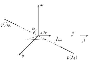
Figure 2: Illustration of elementary transition $\bar{p}(\lambda_{\bar{p}})p(\lambda_{1})\to\chi_{J\nu}$, where $\lambda_{\bar{p}}$, $\lambda_{1}$ and $\nu$ are particle helicities. The picture refers to the c.m. frame of colliding antiproton and proton. The $\tilde{z}$-axis is directed along the c.m. velocity $\bm{\beta}$.

The elementary process $\bar{p}(\lambda_{\bar{p}})p(\lambda_{1})\to\chi_{J\nu}$ is depicted in Fig. 2 in the $\bar{p}p$ center-of-mass (c.m.) frame. Generally, due to a finite transverse momentum of the proton, the direction of the c.m. velocity

$$\bm{\beta}=\frac{\mathbf{p}_{\bar{p}}+\mathbf{p}_{1}}{E_{\bar{p}}+E_{1}}$$ (38)

does not coincide with the original beam direction. Therefore, the transformation from the laboratory frame to the coordinate system shown in Fig. 2 is obtained in the following way. First, we apply the Lorentz boost from the laboratory frame $(x,y,z)$ to the $\bar{p}p$ c.m. frame $(x^{\prime},y^{\prime},z^{\prime})$ such that the antiproton momentum components become

$$\mathbf{p}_{\bar{p}}^{\prime}=\mathbf{p}_{\bar{p}}-\left(E_{\bar{p}}-\frac{\gamma}{\gamma+1}(\mathbf{p}_{\bar{p}}\bm{\beta})\right)\gamma\bm{\beta}~{},$$ (39)

where $\gamma=1/\sqrt{1-\beta^{2}}$. Second, we perform a rotation of coordinate axes $(x^{\prime},y^{\prime},z^{\prime})$ to the new axes $(\tilde{x},\tilde{y},\tilde{z})$ such that the $\tilde{z}$-axis becomes alongated with the c.m. velocity $\bm{\beta}$. If we denote the polar and azimuthal angles defining the direction of the vector $\bm{\beta}$ in the laboratory frame (or equivalently in the $(x^{\prime},y^{\prime},z^{\prime})$ frame) as $(\Theta_{\beta},\phi_{\beta})$ then the rotation can be done about the axis defined by vector $[\mathbf{e}_{z}^{\prime}\times\bm{\beta}]$ by the angle $\Theta_{\beta}$, according to the convention of Refs. Martin et al. (1984); Ridener et al. (1992); Jacob and Wick (1959). In the resulting coordinate system $(\tilde{x},\tilde{y},\tilde{z})$ the cartesian components of the antiproton three-momentum are, therefore, given by the orthogonal matrix transformation (c.f.Varshalovich et al. (1988))

$$\left(\begin{array}[]{l}p_{\bar{p}}^{\tilde{x}}\\ p_{\bar{p}}^{\tilde{y}}\\ p_{\bar{p}}^{\tilde{z}}\end{array}\right)=\left(\begin{array}[]{lll}\cos^{2}\phi_{\beta}\cos\Theta_{\beta}+\sin^{2}\phi_{\beta}&\cos\phi_{\beta}\sin\phi_{\beta}(\cos\Theta_{\beta}-1)&-\cos\phi_{\beta}\sin\Theta_{\beta}\\ \sin\phi_{\beta}\cos\phi_{\beta}(\cos\Theta_{\beta}-1)&\sin^{2}\phi_{\beta}\cos\Theta_{\beta}+\cos^{2}\phi_{\beta}&-\sin\phi_{\beta}\sin\Theta_{\beta}\\ \sin\Theta_{\beta}\cos\phi_{\beta}&\sin\Theta_{\beta}\sin\phi_{\beta}&\cos\Theta_{\beta}\end{array}\right)\left(\begin{array}[]{l}p_{\bar{p}}^{x^{\prime}}\\ p_{\bar{p}}^{y^{\prime}}\\ p_{\bar{p}}^{z^{\prime}}\end{array}\right)~{}.$$ (40)

In the notations of Refs. Martin et al. (1984); Ridener et al. (1992); Jacob and Wick (1959), the formation amplitude of the $\chi_{J}$-charmonium state with helicity $\nu$ is

$$\langle J\nu|B|\Theta\phi,\lambda_{\bar{p}}\lambda_{1}\rangle=\left(\frac{2J+1}{4\pi}\right)^{1/2}B_{\lambda_{\bar{p}}\lambda_{1}}^{J}D^{J}_{\nu\lambda}(\phi,\Theta,-\phi)~{},$$ (41)

where $D^{J}_{\nu\lambda}(\phi,\Theta,-\phi)$ is the rotation matrix, $\lambda=\lambda_{\bar{p}}-\lambda_{1}$ is the net helicity. The angles $(\Theta,\phi)$ in Eq. (41) are the polar and azimuthal angles of the antiproton momentum in the $(\tilde{x},\tilde{y},\tilde{z})$ coordinate system (see Fig. 2), i.e. $\Theta=\arccos[p_{\bar{p}}^{\tilde{z}}/({p_{\bar{p}}^{\tilde{x}}}^{2}+{p_{\bar{p}}^{\tilde{y}}}^{2}+{p_{\bar{p}}^{\tilde{z}}}^{2})^{1/2}]$ and $\phi=\arctan(p_{\bar{p}}^{\tilde{y}}/p_{\bar{p}}^{\tilde{x}})$ ($0\leq\phi<2\pi$). For the zero transverse momentum of the proton the net helicity is conserved since $D^{J}_{\nu\lambda}(0,0,0)=\delta_{\nu\lambda}$. The coefficients $B_{\lambda_{\bar{p}}\lambda_{1}}^{J}$ are normalized as

$$\sum_{\lambda_{\bar{p}}\lambda_{1}}|B_{\lambda_{\bar{p}}\lambda_{1}}^{J}|^{2}=1~{}.$$ (42)

The invariant amplitude is proportional to the amplitude (41)

$$M_{J\nu;\lambda_{\bar{p}}\lambda_{1}}=\kappa_{J}\langle J\nu|B|\Theta\phi,\lambda_{\bar{p}}\lambda_{1}\rangle~{},$$ (43)

where the coefficient $\kappa_{J}$ can be reconstructed from the partial decay width $\Gamma_{\chi_{J}\to\bar{p}p}$ which gives the relation

$$\kappa_{J}=\left(\frac{64\pi^{2}m_{J}^{2}\Gamma_{\chi_{J}\to\bar{p}p}}{\sqrt{m_{J}^{2}-4m^{2}}}\right)^{1/2}~{}.$$ (44)

The partial wave amplitudes $B_{\lambda_{\bar{p}}\lambda_{1}}^{J}$ encode the dynamics of the charmonium formation. It is, however, possible to obtain some general relations from the symmetry considerations Ridener et al. (1992). It follows from the charge conjugation invariance, that $B_{\lambda_{\bar{p}}\lambda_{1}}^{J}=\eta_{c}(-1)^{J}B_{\lambda_{1}\lambda_{\bar{p}}}^{J}$, where $\eta_{c}=(-1)^{L+S}=1$ is the charge parity of the charmonium (for $\chi$-states $L=S=1$). It is convenient to introduce the notations $B_{0}/\sqrt{2}\equiv B_{++}^{J}$ and $B_{1}\equiv B_{+-}^{J}$ for each $J$. Then the charge conjugation invariance leads to the condition $|B_{-+}^{J}|^{2}=|B_{+-}^{J}|^{2}=|B_{1}|^{2}$. The parity invariance of the amplitude (41) gives the relation $B_{\lambda_{\bar{p}}\lambda_{1}}^{J}=\eta_{p}(-1)^{J}B_{-\lambda_{\bar{p}},-\lambda_{1}}^{J}$, where $\eta_{p}=(-1)^{L+1}=1$ is the charmonium parity. This results in to relations $|B_{++}^{J}|^{2}=|B_{--}^{J}|^{2}=|B_{0}|^{2}/2$. Moreover, in the case of $\chi_{1}$, the charge conjugation invariance leads to the condition $B_{0}=0$. The partial wave amplitudes $B_{0}$ and $B_{1}$ are normalized as

$$2|B_{1}|^{2}+|B_{0}|^{2}=1~{}.$$ (45)

The recent experimental data Ambrogiani et al. (2002) for the angular distributions from the $\bar{p}p\to\chi_{c2}\to J/\psi\gamma\to e^{+}e^{-}\gamma$ decay provide the value $|B_{0}|^{2}=0.13\pm 0.08$. The smallness of the transition amplitude for the net helicity zero can be understood as a signature of hadronic helicity conservation for exclusive processes within perturbative QCD with massless quarks and spin-1 gluons Brodsky and Lepage (1981).

In calculations of the products of the matrix elements for the processes $\bar{p}p\to\chi_{J\nu}$ and $\bar{p}p\to\chi_{J_{1}\nu}$ we will assume for simplicity the proton longitudinal momentum to be $p_{1}^{z}=(\Delta_{0}^{J}+\Delta_{0}^{J_{1}})/2$. This approximation is good enough for the present exploratory studies. (More rigorously, in the first amplitude on should set $p_{1}^{z}=\Delta_{0}^{J}$ and in the second amplitude $p_{1}^{z}=\Delta_{0}^{J_{1}}$.) Then, the azimuthal angle $\phi$ will cancel in the final results for the squares of the matrix elements. This can be seen if we use the property of the rotation matrix (c.f. Varshalovich et al. (1988))

$$D_{MM^{\prime}}^{J}(\alpha,\beta,\gamma)=\mbox{e}^{-i\alpha M}d_{MM^{\prime}}^{J}(\beta)\mbox{e}^{-i\gamma M^{\prime}}$$ (46)

with $d_{MM^{\prime}}^{J}(\beta)$ being the real-valued functions. The consequence is that the formulas (29),(31),(33),(34) and (35) derived earlier depend on the combinations

$$M_{J_{1}\nu;\lambda_{\bar{p}}\lambda_{1}}(\mathbf{q}_{t})M_{J\nu;\lambda_{\bar{p}}\lambda_{1}}^{*}(\mathbf{q}_{t}) = \kappa_{J_{1}}\kappa_{J}\frac{\sqrt{(2J_{1}+1)(2J+1)}}{4\pi}B_{\lambda_{\bar{p}}\lambda_{1}}^{J_{1}}B_{\lambda_{\bar{p}}\lambda_{1}}^{J*}$$ (47)

$$\times d_{\nu\lambda}^{J_{1}}(\Theta)d_{\nu\lambda}^{J}(\Theta)~{}.$$

The phases of the helicity amplitudes $B_{\lambda_{\bar{p}}\lambda_{1}}^{J}$ are unknown. We will fix $B_{0}=1$ for $J=0$ and $B_{1}=1/\sqrt{2}$ for $J=1$. In most calculations we will assume the zero phases of the $J=2$ helicity amplitudes, i.e. $B_{0}=\sqrt{0.13}$ and $B_{1}=\sqrt{0.87/2}$. However, we will also test several different choices of the phases of $B_{0}$ and $B_{1}$ for $J=2$ This will influence the interference terms (31),(35) only.

II.5 Transition amplitudes $\chi_{J_{1}}N\to\chi_{J}N$

Following Gerland et al. (1998) we decompose the internal $c\bar{c}$ wave function of the physical $\chi_{J\nu}$-charmonium state in the basis of wave functions with fixed orbital ($L_{z}$) and spin ($S_{z}$) magnetic quantum numbers as

$$|J\nu\rangle=\sum_{L_{z},S_{z}}|1L_{z};1S_{z}\rangle\langle 1L_{z};1S_{z}|J\nu\rangle~{},$$ (48)

where $z$-axis is directed along the charmonium momentum in the target nucleus rest frame (Fermi motion is neglected here). $\langle 1L_{z};1S_{z}|J\nu\rangle$ are the Clebsch-Gordan coefficients. To avoid misunderstanding, we speak here about the internal orbital angular momentum of a $c\bar{c}$-pair. (The projection of the c.m. orbital momentum of the $c\bar{c}$-pair on the $z$-axis is identically zero.) Assuming that the interaction does not change the internal spin and angular momentum of the $c\bar{c}$-pair we can approximate the rescattering amplitude as

$$\langle J\nu|\hat{S}|J_{1}\nu\rangle=\sum_{L_{z},S_{z}}\langle J\nu|1L_{z};1S_{z}\rangle\langle 1L_{z};1S_{z}|\hat{S}|1L_{z};1S_{z}\rangle\langle 1L_{z};1S_{z}|J_{1}\nu\rangle~{},$$ (49)

where the symbols of the initial and final nucleons are dropped for brevity. Assuming that the ratios between diagonal and nondiagonal transitions do not change with increasing transverse momentum transfer Eq.(49) can be rewritten for the invariant matrix elements:

$$M_{J\nu;J_{1}\nu}(\mathbf{q}_{t})=\mbox{e}^{-B_{\chi N}\mathbf{q}_{t}^{2}/2}\sum_{L_{z},S_{z}}\langle J\nu|1L_{z};1S_{z}\rangle M_{L_{z}S_{z}}(0)\langle 1L_{z};1S_{z}|J_{1}\nu\rangle~{}.$$ (50)

In the two-gluon exchange mechanism $B_{\chi N}\simeq 3$ GeV^-2 for the discussed energy range Gerland et al. (2005). For the forward scattering amplitudes at fixed $L_{z}$ and $S_{z}$ we have

$$M_{L_{z}S_{z}}(0)=2ip_{\rm lab}m\sigma_{L_{z}S_{z}}^{\rm tot}(1-i\rho_{\chi N})~{}.$$ (51)

Here $\rho_{\chi N}=\mbox{Re}M_{L_{z}S_{z}}(0)/\mbox{Im}M_{L_{z}S_{z}}(0)$. From the soft Pomeron exchange one has $\rho_{\chi N}\simeq 0.15$, while pQCD gives $\rho_{\chi N}\simeq 0.3$. In numerical calculations we have chosen $\rho_{\chi N}=0.22$, i.e. the average of these two values, since the sensitivity to $\rho_{\chi N}$ in the interval 0.15-0.3 turns out to be quite modest (see the right panel of Fig. 11 below).

The most important input of our calculations are the cross sections $\sigma_{L_{z}S_{Z}}^{\rm tot}\equiv\sigma_{L_{z}}$ which have been calculated in Ref. Gerland et al. (1998) on the basis of the nonrelativistic quark model and the QCD factorization theorem. The following values have been obtained in Gerland et al. (1998): $\sigma_{0}=6.8$ mb and $\sigma_{\pm 1}=15.9$ mb. The cross sections differ by approximately a factor of two, since the transverse size squared of the $c\bar{c}$ configuration with $L_{z}=\pm 1$ is two times larger as compared to the one of the configuration with $L_{z}=0$. The exact ratio $\sigma_{1}/\sigma_{0}$ deviates from two, because the cross sections are obtained in Ref. Gerland et al. (1998) by weighting the probability density distribution of the relative quark coordinate with the transverse-size-dependent interaction cross section of a $c\bar{c}$ pair with a nucleon. The latter cross section was evaluated in Gerland et al. (1998) based on nonperturbative QCD.

In Table 1 we list the transition amplitudes $M_{J\nu;J_{1}\nu}(0)$ for the different values of $J$, $\nu$ and $J_{1}$.

Table 1: Transition amplitude for different initial ($J_{1}$) and final ($J$) total angular momenta and helicities ($\nu$) of the $\chi_{c}$. For $\nu<0$ one should use the relation $M_{J-\nu;J_{1}-\nu}(0)=(-1)^{J+J_{1}}M_{J\nu;J_{1}\nu}(0)$. The quantities $M_{L_{z}}\equiv M_{L_{z}S_{z}}(0),~{}L_{z}=0,1$ denote the amplitudes with fixed value of the $z$-component of the orbital angular momentum neglecting their spin dependence.

$J$	$\nu$	$J_{1}$	$M_{J\nu;J_{1}\nu}(0)$
0	0	0	$(2M_{1}+M_{0})/3$
0	0	1	0
0	0	2	$\sqrt{2}(M_{1}-M_{0})/3$
1	0	1	$M_{1}$
1	0	2	0
1	1	1	$(M_{1}+M_{0})/2$
1	1	2	$(M_{1}-M_{0})/2$
2	0	2	$(M_{1}+2M_{0})/3$
2	1	2	$(M_{1}+M_{0})/2$
2	2	2	$M_{1}$

The nondiagonal transition amplitudes between physical $\chi_{c}$ states are proportional to the difference between the amplitudes with $L_{z}=1$ and $L_{z}=0$. Hence, the nondiagonal transitions are governed by the difference $\sigma_{1}-\sigma_{0}$ which turns out to be nonzero according to the quark model predictions on the structure of the $\chi_{c}$ states and QCD factorization theorem.

II.6 Occupation numbers

The squares of $\chi_{J}$ production amplitudes on a nucleus (c.f. Eq. (20) etc.) are proportional to the coordinate- and momentum-dependent occupation number $f_{1}(\mathbf{X},\mathbf{p})$ of the struck proton which is formally defined as the Wigner function (21). The cross section on the nucleus (8) includes the sum over all possible struck protons ($N_{1}$). Thus, the cross section depends on the total proton occupation number $n(\mathbf{X},\mathbf{p})$ defined as

$$2n(\mathbf{X},\mathbf{p})=\sum_{N_{1}}f_{1}(\mathbf{X},\mathbf{p})~{}.$$ (52)

By introducing the factor of 2 we assumed the spin saturation of the proton system in the nucleus. In the present work we will use a simple expression for $n(\mathbf{X},\mathbf{p})$, which is based on the local Fermi distribution but takes into account the corrections due to the short range NN correlations (SRC):

$$n(\mathbf{X},\mathbf{p})=(1-P_{2})\Theta(p_{F}-p)+\frac{(2\pi)^{3}}{2}\rho_{p}a_{2}|\psi_{D}(p)|^{2}\Theta(p-p_{F})~{}.$$ (53)

Here $\rho_{p}(\mathbf{X})$ is the proton density; $p_{F}(\mathbf{X})=(3\pi^{2}\rho_{p})^{1/3}$ is the proton Fermi momentum; and $P_{2}\simeq 0.25$ is the proton fraction above Fermi surface Frankfurt and Strikman (1981); Frankfurt et al. (2008). The deuteron wave function $\psi_{D}(p)$ in the momentum representation is normalized as

$$4\pi\int\limits_{0}^{+\infty}dpp^{2}|\psi_{D}(p)|^{2}=1~{}.$$ (54)

The coefficient $a_{2}(\mathbf{X})$ is chosen from from the condition

$$P_{2}=4\pi a_{2}\int\limits_{p_{F}}^{+\infty}dpp^{2}|\psi_{D}(p)|^{2}~{}.$$ (55)

For the deuteron wave function we take the result of calculations with the Paris potential Lacombe et al. (1980).

Overall, the in-medium effects should grow with the mass number of a target nucleus. Hence we selected the ²⁰⁸Pb nucleus for the numerical studies below. The density distributions of protons and neutrons have been taken in the two-parameter Fermi parameterization as described in Larionov et al. (2013).

III Numerical results

We calculate the transverse momentum differential cross sections of the $\chi_{J\nu}$ charmonium production

$$\frac{d\sigma_{\bar{p}A\to\chi_{J\nu}(A-1)^{*}}}{d^{2}k_{t}}=\frac{|M|^{2}}{16\pi^{2}p_{\rm lab}^{2}}~{},$$ (56)

which can be obtained by integrating Eq.(8) over the longitudinal momentum $k^{z}$ and replacing $\sqrt{(E_{\bar{p}}+E_{1})^{2}-k_{t}^{2}-m_{J}^{2}}$ by $p_{\rm lab}$ at the final step. $|M|^{2}$ stands for the full matrix element squared for the charmonium production on the nucleus. It is important to note, that in deriving Eq.(56) we implicitly assumed that the contribution of negative $k^{z}$ is strongly suppressed by the rescattering matrix elements which enter in $|M|^{2}$. This allowed us to limit the integration to the positive values of $k^{z}$ only. The cross section (56) is invariant with respect to the change $\nu\to-\nu$, as can be seen from explicit expressions for the different contributions to $|M|^{2}$ in the previous section.

Figures 3-8 show the transverse momentum differential $\chi_{c}$-charmonia production cross sections with the different total angular momenta $J$ and helicities $\nu$. The calculations were performed at an antiproton beam momentum of $p_{\rm lab}=5.553$ GeV/c corresponding to on-shell $\chi_{c1}$ formation in $\bar{p}p$ collisions.

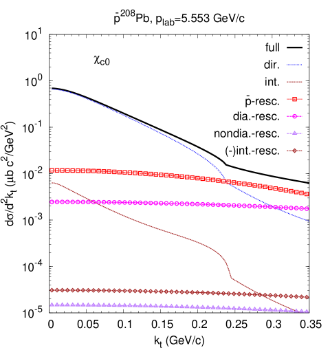
Figure 3: (Color online) Transverse momentum dependence of the differential $\chi_{c0}$ production cross section (56) in $5.553$ GeV/c beam momentum antiproton interactions with the nucleus ²⁰⁸Pb. Full calculation including all contributions to the matrix element is shown by the solid line. Other lines show the partial contributions of the different terms. Direct term (29) – blue dotted line. Interference term (31) – brown dashed line. Antiproton rescattering term (32) – red squares. Diagonal rescattering term (33) – magenta circles. Nondiagonal rescattering term (34) – purple triangles. Interference rescattering term (35) – brown diamonds (contributes with ”-” sign).

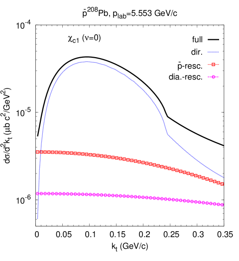
Figure 4: (Color online) Same as Fig. 3, but for $\chi_{c1}$ production with helicity $\nu=0$.

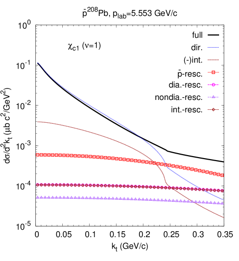
Figure 5: (Color online) Same as Fig. 3, but for $\chi_{c1}$ production with helicity $\nu=1$. The interference term (31) contributes with ”-” sign. The contributions of the diagonal and interference rescattering terms (33), (35) almost coincide with each other.

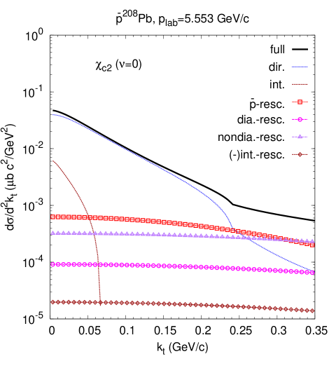
Figure 6: (Color online) Same as Fig. 3, but for $\chi_{c2}$ production with helicity $\nu=0$. The interference rescattering term (35) contributes with ”-” sign.

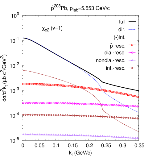
Figure 7: (Color online) Same as Fig. 3, but for $\chi_{c2}$ production with helicity $\nu=1$. The interference term (31) contributes with ”-” sign.

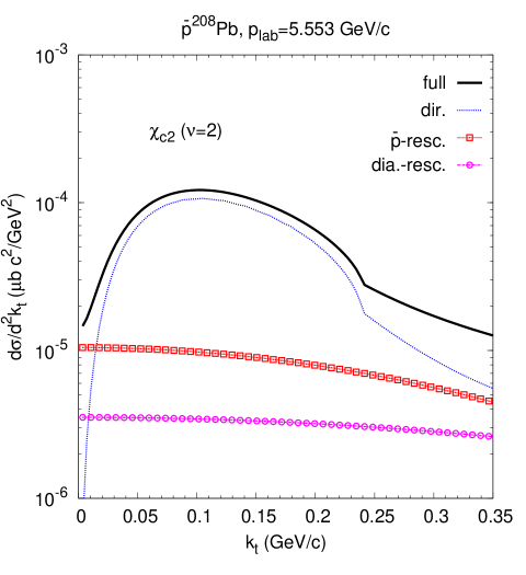
Figure 8: (Color online) Same as Fig. 3, but for $\chi_{c2}$ production with helicity $\nu=2$.

The kinks in the $k_{t}$-dependence at $k_{t}\simeq 0.25$ GeV/c are caused by the sharp change in the momentum dependence of the occupation numbers at the Fermi momentum as discussed in the previous section.

For the states $\chi_{00}$, $\chi_{11}$, $\chi_{20}$ and $\chi_{21}$, whose formation is allowed in $\bar{p}p$ collisions, the cross sections at low $k_{t}$ are dominated by the direct term (29) and at $k_{t}>0.25$ GeV/c – by the term with antiproton rescattering (32). The latter makes the large excess above the SRC tail of the direct term.

The ”exotic” states $\chi_{10}$ and $\chi_{22}$ can not be formed in $\bar{p}p$ collisions and are, therefore, strongly suppressed in antiproton-nucleus collisions. Their production at small $k_{t}$ is mainly caused by the antiproton rescattering term and at $k_{t}>0.25$ GeV/c – by the SRC tail of the direct term. In the latter case the transverse momentum is provided by the target proton. Hence the charmonium spin quantization axis does not coincide with the beam direction anymore ($\Theta>0$ in Eq.(47)). As the consequence, the charmonium helicity may deviate from the difference of the antiproton and proton helicities. The production cross sections of the ”exotic” $\chi_{10}$ and $\chi_{22}$ states on the nucleus are, however, several orders of magnitude lower than for the other ”nonexotic” states $\chi_{00}$, $\chi_{11}$, $\chi_{20}$ and $\chi_{21}$.

We will discuss now the nondiagonal transitions. Note, first, that such transitions do not contribute to the $\chi_{10}$ and $\chi_{22}$ production as one can see from Table 1. On the other hand, the nondiagonal transitions $11\leftrightarrow 21$ and $00\leftrightarrow 20$ do contribute the production of the respective $\chi_{J\nu}$ states. In particular, the transition $00\to 20$ influences the $\chi_{20}$ production at low transverse momenta significantly. This is caused by the large partial partial width $\Gamma_{\chi_{c0}\to\bar{p}p}\simeq 2.3$ keV as compared to $\Gamma_{\chi_{c1}\to\bar{p}p}\simeq 0.06$ keV and $\Gamma_{\chi_{c2}\to\bar{p}p}\simeq 0.14$ keV. As a result, the cross section of $\chi_{20}$ production is enhanced by $\sim 20\%$ at small $k_{t}$ due to the interference term (31).

This is better seen in Fig. 9 which shows the normalized ratio

$${\cal R}=\frac{\chi_{20}}{(\chi_{20}+2\chi_{21})|B_{0}|^{2}}$$ (57)

as a function of $k_{t}$.

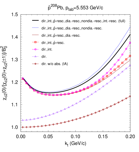
Figure 9: (Color online) The relative contribution ${\cal R}$ (see Eq.(57)) of the $\chi_{c2}$ production with helicity $\nu=0$ to the total $\chi_{c2}$ production in antiproton collisions at 5.553 GeV/c with ²⁰⁸Pb nucleus vs transverse momentum. The normalization is performed on the same contribution $|B_{0}|^{2}=0.13$ in the nonpolarized $\bar{p}p$ collisions.

In the abscence of any in-medium effects (impulse approximation, Eq.(20)) we have ${\cal R}=1$ at $k_{t}=0$. Including absorption (direct term, Eq.(29)) increases ${\cal R}$ by about $5\%$, which reflects the genuine color filtering effect. Indeed, one can see from Table 1 that the absorption cross section of the $\chi_{21}$ state is slightly larger than the absorption cross section of the $\chi_{20}$ state (since $\mbox{Im}M_{1}>\mbox{Im}M_{0}$). The interference term (31) leads to an additional and quite significant enhancement of ${\cal R}$, so that it reaches $\sim 20\%$. The enhancement is not affected by the rescattering terms, which do not influence the ratio ${\cal R}$ at small $k_{t}$, practically.

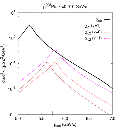
Figure 10: (Color online) Transverse momentum differential cross section of $\chi_{c0}$, $\chi_{c1}$ and $\chi_{c2}$ production with different helicities plotted vs beam momentum at the fixed $k_{t}=0.010$ GeV/c. For orientation, vertical arrows show the beam momenta of the on-shell $\chi_{c0}$, $\chi_{c1}$ and $\chi_{c2}$ formation in $\bar{p}p$ collisions ($p_{\rm lab}=5.194,~{}5.553$ and 5.727 GeV/c, respectively). Note, that the cross sections are peaked at slightly higher beam momenta due the finite value of the nucleon binding energy ($7.9$ MeV for the ²⁰⁸Pb nucleus).

In Fig. 10 we display the beam momentum dependence of the transverse momentum differential cross sections for the ”nonexotic” $\chi_{c}$-states at low transverse momentum . Due to Fermi motion and SRC-correlations there is a strong overlap of the $\chi_{c0}$, $\chi_{c1}$ and $\chi_{c2}$ production in the considered region of beam momenta. This makes possible the interference between these states, since the phase multiplication factor $\Delta_{J_{1}}^{0}-\Delta_{J}^{0}$ in Eq. (31) is small.

Figure 11 shows the beam momentum dependence of the ratio ${\cal R}$ at $k_{t}=0.010$ GeV/c.

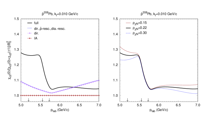
Figure 11: (Color online) The normalized fraction of the $\chi_{c2}$ production with helicity $\nu=0$ (see Eq.(57)) at $k_{t}=0.010$ GeV/c on the ²⁰⁸Pb nucleus as a function of the antiproton beam momentum. Vertical arrows show the beam momenta of the on-shell $\chi_{c0}$, $\chi_{c1}$ and $\chi_{c2}$ formation in $\bar{p}p$ collisions ($p_{\rm lab}=5.194,~{}5.553$ and 5.727 GeV/c, respectively). Left panel shows the calculations with fixed value of $\rho_{\chi N}=0.22$ including combinations of the different terms as indicated. Right panel shows the sensitivity of the full calculation to the choice of parameter $\rho_{\chi N}$ (see Eq.(51))

.

The ratio reaches flat maximum at the beam momentum of about 5.5 GeV/c corresponding to $\Delta_{0}^{0}+\Delta_{2}^{0}=0$, where the occupation number in the interference term (31) is maximal. We also see that ${\cal R}$ drops quickly with increasing beam momentum between $\simeq 5.50$ GeV/c and $\simeq 5.56$ GeV/c. Our results reveal a modest sensitivity to the choice of the ratio of the real and imaginary parts of the $\chi N$-scattering amplitude (right panel of Fig. 11). However, this sensitivity reaches at most $\sim 10\%$ and is visible only for far-off-shell $\chi_{c2}$-production.

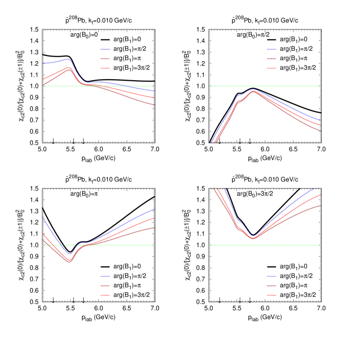
Figure 12: (Color online) Same as in Fig. 11, but for the different values of the phases of $B_{0}$ and $B_{1}$ amplitudes for $J=2$ as indicated.

It is important to note, that all previous results were obtained with the zero phases for the $B_{0}$ and $B_{1}$ helicity amplitudes for $J=2$. Figure 12 shows the sensitivity of the ratio ${\cal R}$ to the choice of phases for the $B_{0}$ and $B_{1}$ amplitudes of $\chi_{2}$ formation in $\bar{p}p$ collisions. The $B_{0}$-phase turns out to be very important: it governs the shape of the beam momentum dependence of ${\cal R}$. The $B_{1}$-phase somewhat shifts ${\cal R}$ vertically but does not influence much the shape of $p_{\rm lab}$-dependence. This is expected since the direct (leading order) contribution to $\chi_{21}$ production is much larger as compared to the direct contribution to $\chi_{20}$ production (compare Figs. 7 and 6). Hence the interference is relatively less important for $\chi_{21}$.

Finally, we would like to make few comments on the possibility of experimental measurements of the polarization effects in the $\chi_{c}$ production at the PANDA@FAIR experiment. The PANDA experimental program The PANDA Collaboration et al. (2009) already includes the studies of the $\bar{p}p\to\chi_{c}\to J/\psi\gamma\to e^{+}e^{-}\gamma$ reaction. The separation of the different $\chi_{c}$ flavors is possible via the different energies of the photon . This can also be done in the case of nuclear target.

For the $\bar{p}A$ reactions, the change in the population of the low $k_{t}$ $\chi_{J\nu}$-states with respect to the one for $\bar{p}p$ reactions will manifest itself in the change of the polar angle distribution of the $J/\psi$-emission for the $\chi_{J}\to J/\psi\gamma$ decay in the $\chi_{J}$ rest frame. Neglecting the $\chi_{2,\pm 2}$ contribution, this distribution can be expressed as

$$W_{J}(\Theta)=\sum_{\nu=\pm 1,0}P_{J\nu}W_{J\nu}(\Theta)~{},$$ (58)

where

$$P_{J\nu}=\frac{\chi_{J\nu}}{\chi_{J0}+2\chi_{J1}}$$ (59)

is the relative fraction of $\chi_{J\nu}$-states. In particular, for $J=2$, $P_{20}={\cal R}|B_{0}|^{2}$, $P_{2,\pm 1}=(1-{\cal R}|B_{0}|^{2})/2$. The polar angle distribution of $J/\psi$’s in the $\chi_{J\nu}$ radiative decay is

$$W_{J\nu}(\Theta)\propto\sum_{\nu^{\prime}=0}^{J}|A^{J}_{\nu^{\prime}}|^{2}([d^{J}_{\nu\nu^{\prime}}(\Theta)]^{2}+[d^{J}_{\nu,-\nu^{\prime}}(\Theta)]^{2})~{}.$$ (60)

This equation includes the helicity amplitudes $A^{J}_{\nu^{\prime}}$ of the radiative decay which can be further expressed via the amplitudes $a_{1},\ldots,a_{J+1}$ of electric or magnetic multipole transitions such that $a_{1},~{}a_{2}$ and $a_{3}$ correspond to E1, M2 and E3 transitions Ridener et al. (1992). The helicity amplitudes $|B_{0}|^{2}$ and $a_{2}$ for $\chi_{c2}$ are experimentally known only with an accuracy of about $30-60\%$ from E835 measurements Ambrogiani et al. (2002). Hence it is very important to perform the polarization studies within the same experimental setup not only for $\bar{p}A$, but also for $\bar{p}p$ reaction. Only such parallel measurements could really address the nuclear effects discussed in the present work.

IV Summary

We have calculated the transverse momentum differential cross sections of the polarized $\chi_{c}$ production in the antiproton-induced reactions on nuclei close to the production threshold. The incoming antiproton was assumed to be unpolarized. We have used the multiple scattering Feynman diagram formalism in the GEA-approach of Refs. Frankfurt et al. (1997); Sargsian (2001). For the elementary amplitudes we used expressions motivated by the phenomenology of $\bar{p}p$-interactions and QCD. The modifications of the proton occupation numbers due to the short-range NN correlations in the nuclear ground state have been taken into account. The calculated differential cross sections have a characteristic two-slope structure. The slope is changed at $k_{t}\simeq 0.25$ GeV/c due to the SRC-tail of the proton momentum distribution at high transverse momenta.

As the polarization observable we have chosen the relative fraction ${\cal R}$ of the $\chi_{c2}$ states with helicity 0 at small transverse momenta normalized such that ${\cal R}=1$ in the $\bar{p}p\to\chi_{c2}$ reaction. The color filtering mechanism alone leads at most to the 10% increase of ${\cal R}$ in $\bar{p}A$ reactions with respect to the $\bar{p}p$ case. The interference of the direct $\bar{p}p\to\chi_{20}$ formation amplitude with the two-step $\bar{p}p\to\chi_{00},\chi_{00}N\to\chi_{20}N$ amplitude strongly influences ${\cal R}$. As a consequence, within a beam momentum range of 5-7 GeV/c, ${\cal R}$ varies by 30-50%. The specific shape of the $p_{\rm lab}$-dependence of ${\cal R}$ is determined by the unknown phase difference of the $B_{0}$ helicity amplitudes for $J=2$ and $J=0$. However, the amplitude of the deviations of ${\cal R}$ from the $\bar{p}p$ value is proportional to the difference between the total interaction cross sections of the 1P charmonium states with $L_{z}=1$ and $L_{z}=0$.

To conclude, we suggest that the experimental measurements of the $p_{\rm lab}$ dependence of the relative fraction of $\chi_{c2}$ states with helicity 0 at small transverse momenta in $\bar{p}A$ reactions would provide a sensitive test of the constituent quark model description of the $\chi_{c}$ states Such studies can be performed in the future PANDA experiment at FAIR.

Appendix A Multiple scattering diagrams

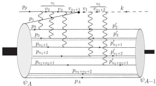
Figure 13: The diagonal transition diagram for the production of the charmonium state $\chi_{J}$ (c.f. Fig. 1a) including multiple elastic rescatterings for the incoming $\bar{p}$ and outgoing $\chi_{J}$.

The diagonal transition term with with $n_{1}$ elastic rescatterings of the antiproton before its annihilation and $n_{2}$ elastic rescatterings of the outgoing charmonium $\chi_{J}$ is shown in Fig. 13. The full transition amplitude (i.e. $S$-matrix element) between the initial state antiproton + nucleus $A$ and final state charmonium + nucleus $(A-1)$ is

$$S_{J\psi_{A-1};\bar{p}\psi_{A}} = \left(\frac{1}{\sqrt{V}}\right)^{2A-1}\int d^{3}x_{2}^{\prime}\cdots d^{3}x_{A}^{\prime}\int d^{3}x_{1}\cdots d^{3}x_{A}$$ (61)

$$\times\psi^{*}_{A-1}(\mathbf{x}_{2}^{\prime},\ldots,\mathbf{x}_{A}^{\prime})\psi_{A}(\mathbf{x}_{1},\mathbf{x}_{2},\ldots,\mathbf{x}_{A})$$

$$\times\int\frac{Vd^{3}p_{2}^{\prime}}{(2\pi)^{3}}\cdots\frac{Vd^{3}p_{n}^{\prime}}{(2\pi)^{3}}\int\frac{Vd^{3}p_{1}}{(2\pi)^{3}}\cdots\frac{Vd^{3}p_{A}}{(2\pi)^{3}}$$

$$\times\mbox{e}^{i\mathbf{p}_{2}^{\prime}\mathbf{x}_{2}^{\prime}+\cdots+i\mathbf{p}_{n}^{\prime}\mathbf{x}_{n}^{\prime}+i\mathbf{p}_{n+1}\mathbf{x}_{n+1}^{\prime}+\cdots+i\mathbf{p}_{A}\mathbf{x}_{A}^{\prime}}$$

$$\times S_{JN_{2}^{\prime}\cdots N_{n}^{\prime};\bar{p}N_{1}\cdots N_{n}}\mbox{e}^{-i\mathbf{p}_{1}\mathbf{x}_{1}-\cdots-i\mathbf{p}_{A}\mathbf{x}_{A}}~{},$$

where $n=n_{1}+n_{2}+1$ is the number of involved nucleons, $S_{JN_{2}^{\prime}\cdots N_{n}^{\prime};\bar{p}N_{1}\cdots N_{n}}$ is the amplitude of the transition between plane-wave states, and $V$ is a normalization volume. Integrating-out the momenta and coordinates of the spectator nucleons in the final state gives the following expression

$$S_{J\psi_{A-1};\bar{p}\psi_{A}} = \left(\frac{1}{\sqrt{V}}\right)^{2n-1}\int d^{3}x_{2}^{\prime}\cdots d^{3}x_{n}^{\prime}\int d^{3}x_{1}\cdots d^{3}x_{A}$$ (62)

$$\times\psi^{*}_{A-1}(\mathbf{x}_{2}^{\prime},\ldots,\mathbf{x}_{n}^{\prime},\mathbf{x}_{n+1},\ldots,\mathbf{x}_{A})\psi_{A}(\mathbf{x}_{1},\ldots,\mathbf{x}_{A})$$

$$\times\int\frac{Vd^{3}p_{2}^{\prime}}{(2\pi)^{3}}\cdots\frac{Vd^{3}p_{n}^{\prime}}{(2\pi)^{3}}\int\frac{Vd^{3}p_{1}}{(2\pi)^{3}}\cdots\frac{Vd^{3}p_{n}}{(2\pi)^{3}}$$

$$\times\mbox{e}^{i\mathbf{p}_{2}^{\prime}\mathbf{x}_{2}^{\prime}+\cdots+i\mathbf{p}_{n}^{\prime}\mathbf{x}_{n}^{\prime}}S_{JN_{2}^{\prime}\cdots N_{n}^{\prime};\bar{p}N_{1}\cdots N_{n}}\mbox{e}^{-i\mathbf{p}_{1}\mathbf{x}_{1}-\cdots-i\mathbf{p}_{n}\mathbf{x}_{n}}~{}.$$

The $S$-matrix element between plane-wave states is expressed as follows

$$S_{JN_{2}^{\prime}\cdots N_{n}^{\prime};\bar{p}N_{1}\cdots N_{n}} = i(2\pi)^{4}\delta^{(4)}(p_{\bar{p}}+p_{1}+p_{2}+\cdots+p_{n}-k-p_{2}^{\prime}-\cdots-p_{n}^{\prime})$$ (63)

$$\times\frac{M_{JN_{2}^{\prime}\cdots N_{n}^{\prime};\bar{p}N_{1}\cdots N_{n}}}{[2E_{\bar{p}}V2E_{1}V(2mV)^{2(n-1)}2\omega V]^{1/2}}~{},$$

where we assumed that the initial and final nucleons are nonrelativistic. For the following it is convenient to introduce the four-momentum transfer by the $i$-th nucleon as

$$q_{i}=p_{i}-p_{i}^{\prime}~{},~{}~{}i=2,\ldots,n~{}.$$ (64)

The corresponding transverse and longitudinal momentum transfers are then $\mathbf{t}_{i}\equiv\mathbf{q}_{it}=\mathbf{p}_{it}-\mathbf{p}_{it}^{\prime}$ and $q_{i}^{z}=p_{i}^{z}-p_{i}^{\prime z}$.

The invariant amplitude is calculated with a help of Feynman rules which gives

$$M_{JN_{2}^{\prime}\cdots N_{n}^{\prime};\bar{p}N_{1}\cdots N_{n}} = \frac{M_{JN}(\mathbf{t}_{n})M_{JN}(\mathbf{t}_{n-1})\cdots M_{JN}(\mathbf{t}_{n_{1}+2})M_{J;\bar{p}p}(\mathbf{p}_{1t})}{D_{J}(v_{n-1})\cdots D_{J}(v_{n_{1}+2})D_{J}(v_{1})}$$ (65)

$$\times\frac{M_{\bar{p}N}(\mathbf{t}_{n_{1}+1})\cdots M_{\bar{p}N}(\mathbf{t}_{2})}{D_{\bar{p}}(v_{n_{1}+1})\cdots D_{\bar{p}}(v_{2})}~{}.$$

We assumed here that the elementary amplitudes depend on the transverse momentum transfers only. The antiproton inverse propagators are

$$-D_{\bar{p}}(v_{i})=(p_{\bar{p}}+\sum_{j=2}^{i}q_{j})^{2}-m^{2}+i\varepsilon=2p_{\rm lab}(-l_{i}+i\varepsilon)~{},~{}~{}i=2,\ldots,n_{1}+1~{}.$$ (66)

The charmonium inverse propagators are

$$-D_{J}(v_{1}) = (p_{\bar{p}}+p_{1}+\sum_{j=2}^{n_{1}+1}q_{j})^{2}-m_{J}^{2}+i\varepsilon=2p_{\rm lab}(\Delta^{0}_{J}-l_{1}+i\varepsilon)~{},$$

$$-D_{J}(v_{i}) = (p_{\bar{p}}+p_{1}+\sum_{j=2}^{i}q_{j})^{2}-m_{J}^{2}+i\varepsilon=2p_{\rm lab}(\Delta^{0}_{J}-l_{i}+i\varepsilon)~{},$$ (67)

where $i=n_{1}+2,\ldots,n-1$. In Eqs.(66),(67) we used the accumulated longitudinal momentum transfers defined as

$$l_{i}=\left\{\begin{array}[]{lll}\sum_{j=2}^{i}q_{j}^{z}&\mbox{for}&i=2,\ldots,n_{1}+1~{},\\ p_{1}^{z}+\sum_{j=2}^{n_{1}+1}q_{j}^{z}&\mbox{for}&i=1~{},\\ p_{1}^{z}+\sum_{j=2}^{i}q_{j}^{z}&\mbox{for}&i=n_{1}+2,\ldots,n-1~{}.\end{array}\right.$$ (68)

By using the coordinate representation of the propagators (15) we can now perform the longitudinal momentum integrations in (62). After some algebra we come to the following expression:

$$\int dp_{2}^{\prime z} \cdots dp_{n}^{\prime z}\int dp_{1}^{z}\cdots dp_{n}^{z}\delta(p_{\rm lab}+p_{1}^{z}+q_{2}^{z}+\cdots+q_{n}^{z}-k^{z})$$ (69)

$$\times\exp\{ip_{2}^{\prime z}z_{2}^{\prime}+\cdots+ip_{n}^{\prime z}z_{n}^{\prime}-il_{2}z_{2}^{0}-\cdots-il_{n_{1}+1}z_{n_{1}+1}^{0}$$

$$\hskip 42.67912pt+i(\Delta^{0}_{J}-l_{1})z_{1}^{0}+i(\Delta^{0}_{J}-l_{n_{1}+2})z_{n_{1}+2}^{0}+\cdots+i(\Delta^{0}_{J}-l_{n_{1}+n_{2}})z_{n_{1}+n_{2}}^{0}$$

$$\hskip 42.67912pt-ip_{1}^{z}z_{1}-\cdots-ip_{n}^{z}z_{n}\}$$

$$= (2\pi)^{n-1}\delta(z_{2}^{\prime}-z_{2})\cdots\delta(z_{n}^{\prime}-z_{n})\exp\{i\Delta^{0}_{J}(z_{1}^{0}+z_{n_{1}+2}^{0}+\cdots+z_{n_{1}+n_{2}}^{0})\}$$

$$\times\int dq_{2}^{z}\cdots dq_{n}^{z}\exp\{-iq_{2}^{z}z_{2}-\cdots-iq_{n}^{z}z_{n}-il_{1}z_{1}^{0}-il_{2}z_{2}^{0}-\cdots-il_{n_{1}+n_{2}}z_{n_{1}+n_{2}}^{0}$$

$$\hskip 99.58464pt+i(p_{\rm lab}-k^{z}+q_{2}^{z}+\cdots+q_{n}^{z})z_{1}\}$$

$$= (2\pi)^{2(n-1)}\delta(z_{2}^{\prime}-z_{2})\cdots\delta(z_{n}^{\prime}-z_{n})\delta(z_{2}-z_{3}+z_{2}^{0})\cdots\delta(z_{n_{1}}-z_{n_{1}+1}+z_{n_{1}}^{0})$$

$$\times\delta(z_{n_{1}+1}-z_{1}+z_{n_{1}+1}^{0})\delta(z_{n_{1}+2}-z_{1}-z_{1}^{0})$$

$$\times\delta(z_{n_{1}+3}-z_{n_{1}+2}-z_{n_{1}+2}^{0})\cdots\delta(z_{n}-z_{n-1}-z_{n-1}^{0})$$

$$\times\exp\{i(p_{\rm lab}-k^{z}+\Delta_{J}^{0})z_{n}-i\Delta_{J}^{0}z_{1}\}~{}.$$

In order to obtain the last expression in (69) we substituted the expression $p_{1}^{z}=k^{z}-p_{\rm lab}-q_{2}^{z}-\cdots-q_{n}^{z}$ in the formulas (68) for the accumulated longitudinal momentum transfers and, after performing the integrations over $dq_{2}^{z}\cdots dq_{n}^{z}$, simplified the arguments of $\delta$-functions by using recursive relations

$$z_{i}+z_{i}^{0}+\cdots+z_{n_{1}+1}^{0}-z_{1}=z_{i}-z_{i+1}+z_{i}^{0}~{},~{}~{}i=n_{1},\ldots,2~{};$$

$$z_{i}-z_{1}^{0}-z_{n_{1}+2}^{0}-\cdots-z_{i-1}^{0}-z_{1}=z_{i}-z_{i-1}-z_{i-1}^{0}~{},~{}~{}i=n_{1}+3,\ldots,n~{}.$$ (70)

Transverse momentum integrations in (62) are performed as follows:

$$\int d^{2}p_{2t}^{\prime} \cdots d^{2}p_{nt}^{\prime}\int d^{2}p_{1t}\cdots d^{2}p_{nt}\delta^{(2)}(\mathbf{p}_{1t}+\mathbf{t}_{2}+\cdots+\mathbf{t}_{n}-\mathbf{k}_{t})$$ (71)

$$\times M_{\bar{p}N}(\mathbf{t}_{2})\cdots M_{\bar{p}N}(\mathbf{t}_{n_{1}+1})M_{J;\bar{p}N}(\mathbf{p}_{1t})M_{JN}(\mathbf{t}_{n_{1}+2})\cdots M_{JN}(\mathbf{t}_{n})$$

$$\times\exp\{i\mathbf{p}_{2t}^{\prime}\mathbf{b}_{2}^{\prime}+\cdots+i\mathbf{p}_{nt}^{\prime}\mathbf{b}_{n}^{\prime}-i\mathbf{p}_{1t}\mathbf{b}_{1}-\cdots-i\mathbf{p}_{nt}\mathbf{b}_{n}\}$$

$$= (2\pi)^{2(n-1)}\delta^{(2)}(\mathbf{b}_{2}^{\prime}-\mathbf{b}_{2})\cdots\delta^{(2)}(\mathbf{b}_{n}^{\prime}-\mathbf{b}_{n})\exp(-i\mathbf{k}_{t}\mathbf{b}_{1})\int d^{2}t_{2}\cdots d^{2}t_{n}$$

$$\times\exp\{-i\mathbf{t}_{2}(\mathbf{b}_{2}-\mathbf{b}_{1})-\cdots-i\mathbf{t}_{n}(\mathbf{b}_{n}-\mathbf{b}_{1})\}M_{\bar{p}N}(\mathbf{t}_{2})\cdots M_{\bar{p}N}(\mathbf{t}_{n_{1}+1})$$

$$\times M_{J;\bar{p}p}(\mathbf{k}_{t}-\mathbf{t}_{2}-\cdots-\mathbf{t}_{n})M_{JN}(\mathbf{t}_{n_{1}+2})\cdots M_{JN}(\mathbf{t}_{n})~{}.$$

We see that due to the $\delta$-functions in Eqs.(69),(71) the primed and nonprimed coordinates coincide and the integration over $d^{3}x_{2}^{\prime}\cdots d^{3}x_{n}^{\prime}$ in Eq. (62) leads to the appearance of the product $\psi^{*}_{A-1}(\mathbf{x}_{2},\ldots,\mathbf{x}_{A})\psi_{A}(\mathbf{x}_{1},\ldots,\mathbf{x}_{A})$ in the transition amplitude.

Using Eqs.(69),(71) and assuming again the nonrelativistic nucleons (i.e. neglecting the energy transfer in rescattering processes) we can rewrite the amplitude (62) as

$$S_{J\psi_{A-1};\bar{p}\psi_{A}}=\frac{i(2\pi)\delta(E_{\bar{p}}+E_{1}-\omega)}{(2E_{\bar{p}}V2\omega V)^{1/2}}M_{J\psi_{A-1};\bar{p}\psi_{A}}~{},$$ (72)

where the matrix element $M_{J\psi_{A-1};\bar{p}\psi_{A}}$ should be replaced by the following one:

$$M^{J}(1,2,\ldots,n) = \frac{i^{n-1}}{(2E_{1})^{1/2}(2\pi)^{2(n-1)}(4mp_{\rm lab})^{n-1}}$$ (73)

$$\times\int d^{3}x_{1}\cdots d^{3}x_{A}\psi^{*}_{A-1}(\mathbf{x}_{2},\ldots,\mathbf{x}_{A})\psi_{A}(\mathbf{x}_{1},\ldots,\mathbf{x}_{A})$$

$$\times\Theta(z_{3}-z_{2})\cdots\Theta(z_{n_{1}+1}-z_{n_{1}})\Theta(z_{1}-z_{n_{1}+1})\Theta(z_{n_{1}+2}-z_{1})$$

$$\times\Theta(z_{n_{1}+3}-z_{n_{1}+2})\cdots\Theta(z_{n}-z_{n-1})$$

$$\times\exp\{i(p_{\rm lab}-k^{z}+\Delta_{J}^{0})z_{n}-i\Delta_{J}^{0}z_{1}-i\mathbf{k}_{t}\mathbf{b}_{1}\}\int d^{2}t_{2}\cdots d^{2}t_{n}$$

$$\times\exp\{-i\mathbf{t}_{2}(\mathbf{b}_{2}-\mathbf{b}_{1})-\cdots-i\mathbf{t}_{n}(\mathbf{b}_{n}-\mathbf{b}_{1})\}M_{\bar{p}N}(\mathbf{t}_{2})\cdots M_{\bar{p}N}(\mathbf{t}_{n_{1}+1})$$

$$\times M_{J;\bar{p}p}(\mathbf{k}_{t}-\mathbf{t}_{2}-\cdots-\mathbf{t}_{n})M_{JN}(\mathbf{t}_{n_{1}+2})\cdots M_{JN}(\mathbf{t}_{n})~{}.$$

The product of $\Theta$-functions in this equation is governed by the order of scatterings of the incoming antiproton and outgoing charmonium. Hence, summing all possible diagrams with the different order of scatterings on the fixed sets of nucleons-scatterers ($n_{1}$ scatterers for the $\bar{p}$ and $n_{2}$ scatterers the for charmonium) is equivalent to the replacement of the product of the $\Theta$-functions in (73) by the following one:

$$\Theta(z_{1}-z_{2})\cdots\Theta(z_{1}-z_{n_{1}+1})\Theta(z_{n_{1}+2}-z_{1})\cdots\Theta(z_{n}-z_{1})~{}.$$ (74)

Let us now constrain the kinematics of the produced charmonium such that $|p_{\rm lab}-k^{z}|\ll p_{\rm lab}$, i.e to the quasifree region. Due to the presence of $\delta(E_{\bar{p}}+E_{1}-\omega)$ in the expressions for the $S$-matrix (72) and in the differential cross section (8), such a constraint leads to the condition

$$p_{\rm lab}-k^{z}+\Delta_{J}^{0}\simeq(\Delta_{J}^{0})^{2}/2p_{\rm lab}\ll\Delta_{J}^{0}~{}.$$ (75)

And thus we can neglect the term $i(p_{\rm lab}-k^{z}+\Delta_{J}^{0})z_{n}$ in the exponent of Eq.(73) which depends on the longitudinal coordinate $z_{n}$ of the last scatterer. This leads us to the following expression for the matrix element of the diagonal transition with multiple elastic rescatterings:

$$M^{J}(1,2,\ldots,n) = \frac{i^{n-1}}{(2E_{1})^{1/2}(2\pi)^{2(n-1)}(4mp_{\rm lab})^{n-1}}\int d^{3}x_{1}\cdots d^{3}x_{A}$$ (76)

$$\times\psi^{*}_{A-1}(\mathbf{x}_{2},\ldots,\mathbf{x}_{A})\psi_{A}(\mathbf{x}_{1},\ldots,\mathbf{x}_{A})\Theta(z_{1}-z_{2})\cdots\Theta(z_{1}-z_{n_{1}+1})$$

$$\times\Theta(z_{n_{1}+2}-z_{1})\cdots\Theta(z_{n}-z_{1})\exp\{-i\Delta_{J}^{0}z_{1}-i\mathbf{k}_{t}\mathbf{b}_{1}\}\int d^{2}t_{2}\cdots d^{2}t_{n}$$

$$\times\exp\{-i\mathbf{t}_{2}(\mathbf{b}_{2}-\mathbf{b}_{1})-\cdots-i\mathbf{t}_{n}(\mathbf{b}_{n}-\mathbf{b}_{1})\}M_{\bar{p}N}(\mathbf{t}_{2})\cdots M_{\bar{p}N}(\mathbf{t}_{n_{1}+1})$$

$$\times M_{J;\bar{p}p}(\mathbf{k}_{t}-\mathbf{t}_{2}-\cdots-\mathbf{t}_{n})M_{JN}(\mathbf{t}_{n_{1}+2})\cdots M_{JN}(\mathbf{t}_{n})~{}.$$

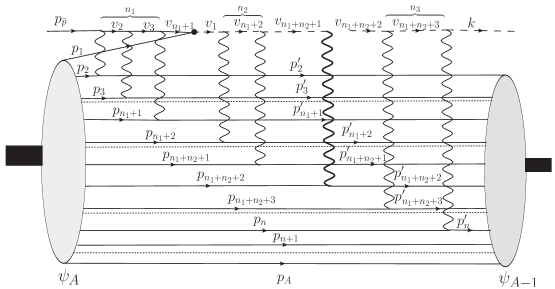
Figure 14: The diagram with one nondiagonal transition $\chi_{J_{1}}N_{n_{1}+n_{2}+2}\to\chi_{J}N_{n_{1}+n_{2}+2}^{\prime}$ (c.f. Fig. 1c) including multiple elastic rescatterings for the incoming $\bar{p}$, intermediate $\chi_{J_{1}}$ and outgoing $\chi_{J}$.

The diagram with one nondiagonal transition, $n_{1}$ elastic rescatterings of the incoming antiproton, $n_{2}$ elastic rescatterings of intermediate charmonium $\chi_{J_{1}}$ and $n_{3}$ elastic rescatterings of the outgoing charmonium $\chi_{J}$ is shown in Fig. 14. In total, $n=n_{1}+n_{2}+n_{3}+2$ nucleons are involved in the reaction. It is clear then, that the formulas (61)-(64) are valid also in this case, but with the newly defined value of $n$. For the invariant amplitude we have now instead of Eq.(65):

$$M_{JN_{2}^{\prime}\cdots N_{n}^{\prime};\bar{p}N_{1}\cdots N_{n}} = \frac{M_{JN}(\mathbf{t}_{n})M_{JN}(\mathbf{t}_{n-1})\cdots M_{JN}(\mathbf{t}_{n_{1}+n_{2}+3})M_{JN;J_{1}N}(\mathbf{t}_{n_{1}+n_{2}+2})}{D_{J}(v_{n-1})\cdots D_{J}(v_{n_{1}+n_{2}+2})}$$ (77)

$$\times\frac{M_{J_{1}N}(\mathbf{t}_{n_{1}+n_{2}+1})\cdots M_{J_{1}N}(\mathbf{t}_{n_{1}+2})M_{J_{1};\bar{p}p}(\mathbf{p}_{1t})}{D_{J_{1}}(v_{n_{1}+n_{2}+1})\cdots D_{J_{1}}(v_{n_{1}+2})D_{J_{1}}(v_{1})}$$

$$\times\frac{M_{\bar{p}N}(\mathbf{t}_{n_{1}+1})\cdots M_{\bar{p}N}(\mathbf{t}_{2})}{D_{\bar{p}}(v_{n_{1}+1})\cdots D_{\bar{p}}(v_{2})}~{}.$$

The antiproton inverse propagators are given by Eq.(66). The $\chi_{J_{1}}$-charmonium inverse propagators are

$$-D_{J_{1}}(v_{1}) = (p_{\bar{p}}+p_{1}+\sum_{j=2}^{n_{1}+1}q_{j})^{2}-m_{J_{1}}^{2}+i\varepsilon=2p_{\rm lab}(\Delta^{0}_{J_{1}}-l_{1}+i\varepsilon)~{},$$

$$-D_{J_{1}}(v_{i}) = (p_{\bar{p}}+p_{1}+\sum_{j=2}^{i}q_{j})^{2}-m_{J_{1}}^{2}+i\varepsilon=2p_{\rm lab}(\Delta^{0}_{J_{1}}-l_{i}+i\varepsilon)~{},$$ (78)

where $i=n_{1}+2,\ldots,n_{1}+n_{2}+1$. The $\chi_{J}$-charmonium inverse propagators are

$$-D_{J}(v_{i}) = (p_{\bar{p}}+p_{1}+\sum_{j=2}^{i}q_{j})^{2}-m_{J}^{2}+i\varepsilon=2p_{\rm lab}(\Delta^{0}_{J}-l_{i}+i\varepsilon)~{},$$ (79)

where $i=n_{1}+n_{2}+2,\ldots,n-1$. The accumulated longitudinal momentum transfers $l_{i}$ are given by Eqs.(68) with the new value of $n$.

The longitudinal momentum integration in (62) becomes now

$$\int dp_{2}^{\prime z} \cdots dp_{n}^{\prime z}\int dp_{1}^{z}\cdots dp_{n}^{z}\delta(p_{\rm lab}+p_{1}^{z}+q_{2}^{z}+\cdots+q_{n}^{z}-k^{z})$$ (80)

$$\times\exp\{ip_{2}^{\prime z}z_{2}^{\prime}+\cdots+ip_{n}^{\prime z}z_{n}^{\prime}-il_{2}z_{2}^{0}-\cdots-il_{n_{1}+1}z_{n_{1}+1}^{0}$$

$$\hskip 42.67912pt+i(\Delta^{0}_{J_{1}}-l_{1})z_{1}^{0}+i(\Delta^{0}_{J_{1}}-l_{n_{1}+2})z_{n_{1}+2}^{0}+\cdots+i(\Delta^{0}_{J_{1}}-l_{n_{1}+n_{2}+1})z_{n_{1}+n_{2}+1}^{0}$$

$$\hskip 42.67912pt+i(\Delta^{0}_{J}-l_{n_{1}+n_{2}+2})z_{n_{1}+n_{2}+2}^{0}+\cdots+i(\Delta^{0}_{J}-l_{n-1})z_{n-1}^{0}-ip_{1}^{z}z_{1}-\cdots-ip_{n}^{z}z_{n}\}$$

$$= (2\pi)^{n-1}\delta(z_{2}^{\prime}-z_{2})\cdots\delta(z_{n}^{\prime}-z_{n})$$

$$\times\exp\{i\Delta^{0}_{J_{1}}(z_{1}^{0}+z_{n_{1}+2}^{0}+\cdots+z_{n_{1}+n_{2}+1}^{0})+i\Delta^{0}_{J}(z_{n_{1}+n_{2}+2}^{0}+\cdots+z_{n-1}^{0})\}$$

$$\times\int dq_{2}^{z}\cdots dq_{n}^{z}\exp\{-iq_{2}^{z}z_{2}-\cdots-iq_{n}^{z}z_{n}-il_{1}z_{1}^{0}-\cdots-il_{n-1}z_{n-1}^{0}$$

$$\hskip 99.58464pt+i(p_{\rm lab}-k^{z}+q_{2}^{z}+\cdots+q_{n}^{z})z_{1}\}$$

$$= (2\pi)^{2(n-1)}\delta(z_{2}^{\prime}-z_{2})\cdots\delta(z_{n}^{\prime}-z_{n})\delta(z_{2}-z_{3}+z_{2}^{0})\cdots\delta(z_{n_{1}}-z_{n_{1}+1}+z_{n_{1}}^{0})$$

$$\times\delta(z_{n_{1}+1}-z_{1}+z_{n_{1}+1}^{0})\delta(z_{n_{1}+2}-z_{1}-z_{1}^{0})$$

$$\times\delta(z_{n_{1}+3}-z_{n_{1}+2}-z_{n_{1}+2}^{0})\cdots\delta(z_{n}-z_{n-1}-z_{n-1}^{0})$$

$$\times\exp\{i(p_{\rm lab}-k^{z}+\Delta_{J}^{0})z_{n}-i\Delta_{J_{1}}^{0}z_{1}+i(\Delta_{J_{1}}^{0}-\Delta_{J}^{0})z_{n_{1}+n_{2}+2}\}~{}.$$

The derivation of the last expression in (80) was performed in full analogy with the case of the longitudinal integral (69) for the diagonal amplitude. We again used the formulas (68) for the accumulated longitudinal momentum transfers with $p_{1}^{z}=k^{z}-p_{\rm lab}-q_{2}^{z}-\cdots-q_{n}^{z}$ and applied the recursive relations (70) in the arguments of the $\delta$-functions (with newly defined $n=n_{1}+n_{2}+n_{3}+2$).

Transverse momentum integral in (62) for the nondiagonal amplitude has the following form:

$$\int d^{2}p_{2t}^{\prime} \cdots d^{2}p_{nt}^{\prime}\int d^{2}p_{1t}\cdots d^{2}p_{nt}\delta^{(2)}(\mathbf{p}_{1t}+\mathbf{t}_{2}+\cdots+\mathbf{t}_{n}-\mathbf{k}_{t})M_{\bar{p}N}(\mathbf{t}_{2})\cdots M_{\bar{p}N}(\mathbf{t}_{n_{1}+1})$$ (81)

$$\times M_{J_{1};\bar{p}p}(\mathbf{p}_{1t})M_{J_{1}N}(\mathbf{t}_{n_{1}+2})\cdots M_{J_{1}N}(\mathbf{t}_{n_{1}+n_{2}+1})M_{JN;J_{1}N}(\mathbf{t}_{n_{1}+n_{2}+2})$$

$$\times M_{JN}(\mathbf{t}_{n_{1}+n_{2}+3})\cdots M_{JN}(\mathbf{t}_{n})\exp\{i\mathbf{p}_{2t}^{\prime}\mathbf{b}_{2}^{\prime}+\cdots+i\mathbf{p}_{nt}^{\prime}\mathbf{b}_{n}^{\prime}-i\mathbf{p}_{1t}\mathbf{b}_{1}-\cdots-i\mathbf{p}_{nt}\mathbf{b}_{n}\}$$

$$= (2\pi)^{2(n-1)}\delta^{(2)}(\mathbf{b}_{2}^{\prime}-\mathbf{b}_{2})\cdots\delta^{(2)}(\mathbf{b}_{n}^{\prime}-\mathbf{b}_{n})\exp(-i\mathbf{k}_{t}\mathbf{b}_{1})\int d^{2}t_{2}\cdots d^{2}t_{n}$$

$$\times\exp\{-i\mathbf{t}_{2}(\mathbf{b}_{2}-\mathbf{b}_{1})-\cdots-i\mathbf{t}_{n}(\mathbf{b}_{n}-\mathbf{b}_{1})\}M_{\bar{p}N}(\mathbf{t}_{2})\cdots M_{\bar{p}N}(\mathbf{t}_{n_{1}+1})$$

$$\times M_{J_{1};\bar{p}p}(\mathbf{k}_{t}-\mathbf{t}_{2}-\cdots-\mathbf{t}_{n})M_{J_{1}N}(\mathbf{t}_{n_{1}+2})\cdots M_{J_{1}N}(\mathbf{t}_{n_{1}+n_{2}+1})$$

$$\times M_{JN^{\prime};J_{1}N}(\mathbf{t}_{n_{1}+n_{2}+2})M_{JN}(\mathbf{t}_{n_{1}+n_{2}+3})\cdots M_{JN}(\mathbf{t}_{n})~{}.$$

Using (80),(81) we can express the amplitude of the nondiagonal transition including multiple elastic rescatterings in the form (72) with the matrix element $M_{J\psi_{A-1};\bar{p}\psi_{A}}$ replaced by

$$M^{J_{1}J}(1,2,\ldots,n) = \frac{i^{n-1}}{(2E_{1})^{1/2}(2\pi)^{2(n-1)}(4mp_{\rm lab})^{n-1}}\int d^{3}x_{1}\cdots d^{3}x_{A}$$ (82)

$$\times\psi^{*}_{A-1}(\mathbf{x}_{2},\ldots,\mathbf{x}_{A})\psi_{A}(\mathbf{x}_{1},\ldots,\mathbf{x}_{A})\Theta(z_{1}-z_{2})\cdots\Theta(z_{1}-z_{n_{1}+1})$$

$$\times\Theta(z_{n_{1}+2}-z_{1})\Theta(z_{n_{1}+n_{2}+2}-z_{n_{1}+2})\cdots\Theta(z_{n_{1}+n_{2}+1}-z_{1})\Theta(z_{n_{1}+n_{2}+2}-z_{n_{1}+n_{2}+1})$$

$$\times\Theta(z_{n_{1}+n_{2}+3}-z_{n_{1}+n_{2}+2})\cdots\Theta(z_{n}-z_{n_{1}+n_{2}+2})$$

$$\times\exp\{-i\Delta_{J_{1}}^{0}z_{1}-i\mathbf{k}_{t}\mathbf{b}_{1}+i(\Delta_{J_{1}}^{0}-\Delta_{J}^{0})z_{n_{1}+n_{2}+2}\}\int d^{2}t_{2}\cdots d^{2}t_{n}$$

$$\times\exp\{-i\mathbf{t}_{2}(\mathbf{b}_{2}-\mathbf{b}_{1})-\cdots-i\mathbf{t}_{n}(\mathbf{b}_{n}-\mathbf{b}_{1})\}M_{\bar{p}N}(\mathbf{t}_{2})\cdots M_{\bar{p}N}(\mathbf{t}_{n_{1}+1})$$

$$\times M_{J_{1};\bar{p}p}(\mathbf{k}_{t}-\mathbf{t}_{2}-\cdots-\mathbf{t}_{n})M_{J_{1}N}(\mathbf{t}_{n_{1}+2})\cdots M_{J_{1}N}(\mathbf{t}_{n_{1}+n_{2}+1})$$

$$\times M_{JN^{\prime};J_{1}N}(\mathbf{t}_{n_{1}+n_{2}+2})M_{JN}(\mathbf{t}_{n_{1}+n_{2}+3})\cdots M_{JN}(\mathbf{t}_{n})~{},$$

where we summed the diagrams with the different order of rescatterings (with the fixed struck nucleon $N_{1}$ and nucleon $N_{n_{1}+n_{2}+2}$ on which the nondiagonal transition takes place) and made the assumption of the quasifree kinematics $|p_{\rm lab}-k^{z}|\ll p_{\rm lab}$ of the final $\chi_{J}$. Equations (76),(82) are the generalizations of the corresponding Eqs.(1),(4) for the case of multiple elastic rescatterings of the antiproton and charmonia.