Asymptotic Stability of POD based Model Predictive Control for a semilinear parabolic PDE

Abstract

In this article a stabilizing feedback control is computed for a semilinear parabolic partial differential equation utilizing a nonlinear model predictive (NMPC) method. In each level of the NMPC algorithm the finite time horizon open loop problem is solved by a reduced-order strategy based on proper orthogonal decomposition (POD). A stability analysis is derived for the combined POD-NMPC algorithm so that the lengths of the finite time horizons are chosen in order to ensure the asymptotic stability of the computed feedback controls. The proposed method is successfully tested by numerical examples.

1 Introduction

In many control problems it is desired to design a stabilizing feedback control, but often the closed-loop solution can not be found analytically, even in the unconstrained case since it involves the solution of the corresponding Hamilton-Jacobi-Bellman equations; see, e.g., [7, 11] and [22]. But this approach requires the solution of a nonlinear hyperbolic partial differential equation with a high-dimensional spatial variable.

One approach to circumvent this problem is the repeated solution of open-loop optimal control problems. The first part of the resulting open-loop input signal is implemented and the whole process is repeated. Control approaches using this strategy are referred to as model predictive control (MPC), moving horizon control or receding horizon control. In general one distinguishes between linear and nonlinear MPC (NMPC). In linear MPC, linear models are used to predict the system dynamics and considers linear constraints on the states and inputs. Note that even if the system is linear, the closed loop dynamics are nonlinear due to the presence of constraints. NMPC refers to MPC schemes that are based on nonlinear models and/or consider a nonquadratic cost functional and general nonlinear constraints. Although linear MPC has become an increasingly popular control technique used in industry, in many applications linear models are not sufficient to describe the process dynamics adequately and nonlinear models must be applied. This inadequacy of linear models is one of the motivations for the increasing interest in nonlinear MPC; see. e.g., [3, 12, 15, 24]. The prediction horizon plays a crucial role in MPC algorithms. For instance, the quasi infinite horizon NMPC allows an efficient formulation of NMPC while guaranteeing stability and the performances of the closed-loop as shown in [4, 13, 19] under appropriate assumptions. For the purpose of our paper we will use a different approach since we will not deal with terminal constraints.

Since the computational complexity of NMPC schemes grows rapidly with the length of the optimization horizon, estimates for minimal stabilizing horizons are of particular interest to ensure stability while being computationally fast. Stability and suboptimality analysis for NMPC schemes without stabilizing constraints are studied in [15, Chapter 6], where the authors give sufficient conditions ensuring asymptotic stability with minimal finite prediction horizon. Note that the stabilization of the problem and the computation of the minimal horizon involve the (relaxed) dynamic programming principle (DPP); see [16, 23]. This approach allows estimates of the finite prediction horizon based on controllability properties of the dynamical system.

Since several optimization problems have to be solved in the NMPC method, it is reasonable to apply reduced-order methods to accelerate the NMPC algorithm. Here, we utilize proper orthogonal decomposition (POD) to derive reduced-order models for nonlinear dynamical systems; see, e.g., [18, 28] and [17]. The application of POD is justified by an a priori error analysis for the considered nonlinear dynamical system, where we combine techniques from [20, 21] and [27]. Let us refer to [14], where the authors also combine successfully an NMPC scheme with a POD reduced-order approach. However, no analysis is carried out ensuring the asymptotic stability of the proposed NMPC-POD scheme. Our contribution focusses on the stability analysis of the POD-NMPC algorithm without terminal constraints, where the dynamical system is a semilinear parabolic partial differential equation with an advection term. In particular, we study a minimal finite horizon for the reduced-order approximation such that it guarantees the asymptotic stability of the surrogate model. Our approach is motivated by the work [6]. The main difference here is that we have added an advection term in the dynamical system and utilize a POD suboptimal strategy to solve the open-loop problems. Since the minimal prediction horizon can be large, the numerical solution of the open-loop problems is very expensive within the NMPC algorithm. The application of the POD model reduction reduces efficiently the computational cost by computing suboptimal solutions. But we involve this suboptimality in our stability analysis in order to ensure the asymptotic stability of our NMPC scheme.

The paper is organized in the following manner: In Section 2 we formulate our infinite horizon optimal control problem governed by a semilinear parabolic equation and bilateral control constraints. The NMPC algorithm is introduced in Section 3. For the readers convenience, we recall the known results of the stability analysis. Further, the stability theory is applied to our underlying nonlinear semilinear equations and bilateral control constraints. In Section 4 we investigate the finite horizon open loop problem which has to be solved at each level of the NMPC algorithm. Moreover, we introduce the POD reduced-order approach and prove an a-priori error estimate for the semilinear parabolic equation. Finally, numerical examples are presented in Section 5.

2 Formulation of the control system

Let $\Omega=(0,1)\subset\mathbb{R}$ be the spatial domain. For the initial time $t_{\circ}\in\mathbb{R}^{+}_{0}=\{s\in\mathbb{R}\,|\,s\geq 0\}$ we define the space-time cylinder $Q=\Omega\times(t_{\circ},\infty)$. By $H=L^{2}(\Omega)$ we denote the Lebesgue space of (equivalence classes of) functions which are (Lebesgue) measurable and square integrable. We endow $H$ by the standard inner product – denoted by $\langle\cdot\,,\cdot\rangle_{H}$ – and the associated induced norm $\|\varphi\|_{H}=\langle\varphi,\varphi\rangle_{H}^{1/2}$. Furthermore, $V=H^{1}_{0}(\Omega)\subset H$ stands for the Sobolev space

$$V=\bigg{\{}\varphi\in H\,\Big{|}\,\int_{\Omega}\big{|}\varphi^{\prime}(x)\big{|}^{2}\,\mathrm{d}x<\infty\text{ and }\varphi(0)=\varphi(1)=0\bigg{\}}.$$

Recall that both $H$ and $V$ are Hilbert spaces. In $V$ we use the inner product

$${\langle\varphi,\phi\rangle}_{V}=\int_{\Omega}\varphi^{\prime}(x)\phi^{\prime}(x)\,\mathrm{d}x\quad\text{for }\varphi,\phi\in V$$

and set $\|\varphi\|_{V}=\langle\varphi,\varphi\rangle_{V}^{1/2}$ for $\varphi\in V$. For more details on Lebesgue and Sobolev spaces we refer the reader to [11], for instance. When the time $t$ is fixed for a given function $\varphi:Q\to\mathbb{R}$, the expression $\varphi(t)$ stands for a function $\varphi(\cdot\,,t)$ considered as a function in $\Omega$ only. Recall that the Hilbert space $L^{2}(Q)$ can be identified with the Bochner space $L^{2}(t_{\circ},\infty;H)$.

We consider the following control system governed by a semilinear parabolic partial differential equation: $y=y(x,t)$ solves the semilinear initial boundary value problem

$$y_{t}-\theta y_{xx}+y_{x}+\rho(y^{3}-y) =u \text{in }Q,$$ (2.1a)

$$y(0,\cdot)=y(1,\cdot) =0 \text{in }(t_{\circ},\infty),$$ (2.1b)

$$y(t_{\circ}) =y_{\circ} \text{in }\Omega.$$ (2.1c)

In (2.1a) it is assumed that the control $u=u(x,t)$ belongs to the set of admissible control inputs

$$\mathbb{U}_{ad}(t_{\circ})=\big{\{}u\in\mathbb{U}(t_{\circ})\,\big{|}\,u(x,t)\in U_{ad}\text{ for almost all (f.a.a.) }(x,t)\in Q\big{\}},$$ (2.2)

where $\mathbb{U}(t_{\circ})=L^{2}(t_{\circ},\infty;H)$ and $U_{ad}=\{u\in\mathbb{R}\,|\,u_{a}\leq u\leq u_{b}\}$ with given $u_{a}\leq 0\leq u_{b}$ . The parameters $\theta$ and $\rho$ satisfy

$$(\theta,\rho)\in D_{ad}=\big{\{}(\tilde{\theta},\tilde{\rho})\in\mathbb{R}^{2}\,\big{|}\,\theta_{a}\leq\tilde{\theta}\text{ and }\rho_{a}\leq\tilde{\rho}\big{\}}$$

with positive $\theta_{a}$ and $\rho_{a}$. Further, in (2.1c) the initial condition $y_{\circ}=y_{\circ}(x)$ is supposed to belong to $H$.

A solution to (2.1) is interpreted in the weak sense as follows: for given $(t_{\circ},y_{\circ})\in\mathbb{R}^{+}_{0}\times H$ and $u\in\mathbb{U}_{ad}(t_{\circ})$ we call $y$ a weak solution to (2.1) for fixed $(\theta,\rho)\in D_{ad}$ if $y(t)\in V$, $y_{t}(t)\in V^{\prime}$ hold f.a.a. $t\geq t_{\circ}$ and $y$ satisfies $y(t_{\circ})=y_{\circ}$ in $H$ as well as

$$\frac{\mathrm{d}}{\mathrm{d}t}\,{\langle y(t),\varphi\rangle}_{H}+\int_{\Omega}\theta y_{x}(t)\varphi^{\prime}+\big{(}y_{x}(t)+\rho(y^{3}(t)-y(t))\big{)}\varphi\,\mathrm{d}x=\int_{\Omega}u(t)\varphi\,\mathrm{d}x$$ (2.3)

for all $\varphi\in V$ and f.a.a. $t>t_{\circ}$. Here, $y_{t}(t)$ stands for the distributional derivative with respect to the time variable satisfying [10, p. 477]

$$\frac{\mathrm{d}}{\mathrm{d}t}\,{\langle y(t),\varphi\rangle}_{H}={\langle y_{t}(t),\varphi\rangle}_{V^{\prime},V}\quad\text{for all }\varphi\in V.$$

The following result is proved in [8], for instance.

Proposition 2.1.

For given $(t_{\circ},y_{\circ})\in\mathbb{R}^{+}_{0}\times H$ and $u\in\mathbb{U}_{ad}(t_{\circ})$ there exists a unique weak solution $y=y_{[u,t_{\circ},y_{\circ}]}$ to (2.1) for every $(\theta,\rho)\in D_{ad}$.

Let $(t_{\circ},y_{\circ})\in\mathbb{R}^{+}_{0}\times H$ be given. Due to Proposition 2.1 we can define the quadratic cost functional:

$$\hat{J}(u;t_{\circ},y_{\circ}):=\frac{1}{2}\int_{t_{\circ}}^{\infty}{\|y_{[u,t_{\circ},y_{\circ}]}(t)-y_{d}\|}_{H}^{2}\,\mathrm{d}t+\frac{\lambda}{2}\int_{t_{\circ}}^{\infty}{\|u(t)\|}_{H}^{2}\,\mathrm{d}t$$ (2.4)

for all $u\in\mathbb{U}(t_{\circ})\supset\mathbb{U}_{ad}(t_{\circ})$, where $y_{[u,t_{\circ},y_{\circ}]}$ denotes the unique weak solution to (2.1). We suppose that $y_{d}=y_{d}(x)$ is a given desired stationary state in $H$ (e.g., the equilibrium $y_{d}=0$) and that $\lambda>0$ denotes a fixed weighting parameter. Then we consider the nonlinear infinite horizon optimal control problem

$$\min\hat{J}(u;t_{\circ},y_{\circ})\quad\text{subject to (s.t.)}\quad u\in\mathbb{U}_{ad}(t_{\circ}).$$ (2.5)

Suppose that the trajectory $y$ is measured at discrete time instances

$$t_{n}=t_{\circ}+n\Delta t,\quad n\in\mathbb{N},$$

where the time step $\Delta t>0$ stands for the time step between two measurements. Thus, we want to select a control $u\in\mathbb{U}_{ad}(t)$ such that the associated trajectory $y_{[u,t_{\circ},y_{\circ}]}$ follows a given desired state $y_{d}$ as good as possible. This problem is called a tracking problem, and, if $y_{d}=0$ holds, a stabilization problem.

Since our goal is to be able to react to the current deviation of the state $y$ at time $t=t_{n}$ from the given reference value $y_{d}$, we would like to have the control in feedback form, i.e., we want to determine a mapping $\mu:H\to\mathbb{U}_{ad}(t_{\circ})$ with $u(t)=\mu(y(t))$ for $t\in[t_{n},t_{n+1}]$.

3 Nonlinear model predictive control

We present an NMPC approach to compute a mapping $\mu$ which allows a representation of the control in feedback form. For more details we refer the reader to the monographs [15, 24], for instance.

3.1 The NMPC method

To introduce the NMPC algorithm we write the weak form of our control system (2.1) as a parametrized nonlinear dynamical system. For $(\theta,\rho)\in D_{ad}$ let us introduce the $\theta$-and $\rho$-dependent nonlinear mapping $\mathcal{F}$ which maps the space $V\times H$ into the dual space $V^{\prime}$ of $V$ as follows:

$$\mathcal{F}(\varphi,v)=-\theta\varphi_{xx}+\varphi_{x}+\rho(\varphi^{3}-\varphi)-v\quad\text{for }(\varphi,v)\in V\times H.$$

Then, we can express (2.3) as the nonlinear dynamical system

$$y^{\prime}(t)=\mathcal{F}(y(t),u(t))\in V^{\prime}\text{ for all }t>t_{\circ},\quad y(t_{\circ})=y_{\circ}\text{ in }H$$ (3.1)

for given $(t_{\circ},y_{\circ})\in\mathbb{R}^{+}_{0}\times H$. The cost functional has been already introduced in (2.4). Summarizing, we want to solve the following infinite horizon minimization problem

$$\min\hat{J}(u;t_{\circ},y_{\circ})=\int_{t_{\circ}}^{\infty}\ell\big{(}y_{[u,t_{\circ},y_{\circ}]}(t),u(t)\big{)}\,\mathrm{d}t\quad\text{s.t.}\quad u\in\mathbb{U}_{ad}(t_{\circ}), \mathbf{P(}t_{\circ}\mathbf{)}$$ ()

where we have defined the running quadratic cost as

$$\ell(\varphi,v)=\frac{1}{2}\left({\|\varphi-y_{d}\|}^{2}_{H}+\lambda\,{\|v\|}_{H}^{2}\right)\quad\text{for }\varphi,v\in H.$$ (3.2)

If we have determined a state feedback $\mu$ for ($\mathbf{P(}t_{\circ}\mathbf{)}$), the control $u(t)=\mu(y(t))$ allows a closed loop representation for $t\in[t_{\circ},\infty)$. Then, for a given initial condition $y_{0}\in H$ we set $t_{\circ}=0$, $y_{\circ}=y_{0}$ in (3.1) and insert $\mu$ to obtain the closed-loop form

$$y^{\prime}(t)=\mathcal{F}(y(t),\mu(y(t))) \text{in }V^{\prime}\text{ for }t\in(t_{\circ},\infty),$$ (3.3)

$$y(t_{\circ})=y_{\circ} \text{in }H.$$

Note that the infinite horizon problem may be very hard to solve due to the dimensionality of the problem. On the other hand it guarantees the stabilization of the problem which is very important for certain applications. In an NMPC algorithm a state feedback law is computed for ($\mathbf{P(}t_{\circ}\mathbf{)}$) by solving a sequence of finite time horizon problems.

To formulate the NMPC algorithm we introduce the finite horizon quadratic cost functional as follows: for $(t_{\circ},y_{\circ})\in\mathbb{R}^{+}_{0}\times H$ and $u\in\mathbb{U}_{ad}^{N}(t_{\circ})$ we set

$$\hat{J}^{N}(u;t_{\circ},y_{\circ})=\int_{t_{\circ}}^{t_{\circ}^{N}}\ell\big{(}y_{[u,t_{\circ},y_{\circ}]}(t),u(t)\big{)}\,\mathrm{d}t,$$

where $N$ is a natural number, $t_{\circ}^{N}=t_{\circ}+N\Delta t$ is the final time and $N\Delta t$ denotes the length of the time horizon for the chosen time step $\Delta t>0$. Further, we introduce the Hilbert space $\mathbb{U}^{N}(t_{\circ})=L^{2}(t_{\circ},t_{\circ}^{N};H)$ and the set of admissible controls

$$\mathbb{U}_{ad}^{N}(t_{\circ})=\big{\{}u\in\mathbb{U}^{N}(t_{\circ})\,\big{|}\,u(x,t)\in U_{ad}\text{ f.a.a. }(x,t)\in Q^{N}\big{\}}$$

with $Q^{N}=\Omega\times(t_{\circ},t_{\circ}^{N})\subset Q$; compare (2.2). In Algorithm 1 the method is presented.

Algorithm 1 (NMPC algorithm)

0:  time step $\Delta t>0$, finite horizon $N\in\mathbb{N}$, weighting parameter $\lambda>0$.

1:  for $n=0,1,2,\ldots$ do

2:     Measure the state $y(t_{n})\in V$ of the system at $t_{n}=n\Delta t$.

3:     Set $t_{\circ}=t_{n}=n\Delta t$, $y_{\circ}=y(t_{n})$ and compute a global solution to

$$\min\hat{J}^{N}(u;t_{\circ},y_{\circ})\quad\text{s.t.}\quad u\in\mathbb{U}_{ad}^{N}(t_{\circ}). \mathbf{P^{\boldsymbol{N}}(}t_{\circ}\mathbf{)}$$ ()

We denote the obtained optimal control by $\bar{u}^{N}$.

4:     Define the NMPC feedback value $\mu^{N}(t;t_{\circ},y_{\circ})=\bar{u}^{N}(t)$, $t\in(t_{\circ},t_{\circ}+\Delta t]$ and use this control to compute the associated state $y=y_{[\mu^{N}(\cdot),t_{\circ},y_{\circ}]}$ by solving (3.1) on $[t_{\circ},t_{\circ}+\Delta t]$.

5:  end for

We store the optimal control on the first subinterval $[t_{\circ},t_{\circ}+\Delta t]=[0,\Delta t]$ and the associated optimal trajectory. Then, we initialize a new finite horizon optimal control problem whose initial condition is given by the optimal trajectory $\bar{y}(t)=y_{[\mu^{N}(\cdot),t_{\circ},y_{\circ}]}(t)$ at $t=t_{\circ}+\Delta t$ using the optimal control $\mu^{N}(t;t_{\circ},y_{\circ})=\bar{u}^{N}(t)$ for $t\in(t_{\circ},t_{\circ}+\Delta t]$ . We iterate this process by setting $t_{\circ}=t_{\circ}+\Delta t$. Of course, the larger the horizon, the better the approximation one can have, but we would like to have the minimal horizon which can guarantee stability [16]. Note that ($\mathbf{P^{\boldsymbol{N}}(}t_{\circ}\mathbf{)}$) is an open loop problem on a finite time horizon $[t_{\circ},t_{\circ}+N\Delta t]$ which will be studied in Section 4.

3.2 Dynamic programming principle (DPP) and asymptotic stability

For the reader’s convenience we now recall the essential theoretical results from dynamic programming and stability analysis. Let us first introduce the so called value function $v$ defined as follows for an infinite horizon optimal control problem:

$$v(t_{\circ},y_{\circ}):=\inf_{u\in\mathbb{U}_{ad}(t_{\circ})}\hat{J}(u;t_{\circ},y_{\circ})\quad\text{for }(t_{\circ},y_{\circ})\in\mathbb{R}_{0}^{+}\times H.$$

Let $N\in\mathbb{N}$ be chosen. The DDP states that the value function $v$ satisfies for any $k\in\{1,\ldots,N\}$ with $t_{\circ}^{k}=t_{k}+k\Delta t$:

$$v(t_{\circ},y_{\circ})$$

$$=\inf_{u\in\mathbb{U}_{ad}^{k}(t_{\circ})}\left\{\int_{t_{\circ}}^{t_{\circ}^{k}}\ell\big{(}y_{[u,t_{\circ},y_{\circ}]}(t),u(t)\big{)}\,\mathrm{d}t+v\big{(}t_{\circ}+k\Delta t,y_{[u,t_{\circ},y_{\circ}]}(t_{\circ}+k\Delta t)\big{)}\right\}$$

which holds under very general conditions on the data; see, e.g., [7] for more details. The value function for the finite horizon problem ($\mathbf{P^{\boldsymbol{N}}(}t_{\circ}\mathbf{)}$) is of the following form:

$$v^{N}(t_{\circ},y_{\circ})=\inf_{u\in\mathbb{U}_{ad}^{N}(t_{\circ})}\hat{J}^{N}(u;t_{\circ},y_{\circ})\quad\text{for }(t_{\circ},y_{\circ})\in\mathbb{R}^{+}_{0}\times H.$$

The value function $v^{N}$ satisfies the DPP for the finite horizon problem for $t_{\circ}+k\Delta t$, $0<k<N$:

$$v^{N}(t_{\circ},y_{\circ})$$

$$\quad=\inf_{u\in\mathbb{U}_{ad}^{k}(t_{\circ})}\left\{\int_{t_{\circ}}^{t_{\circ}+k\Delta t}\ell\big{(}y_{[u,t_{\circ},y_{\circ}]}(t),u(t)\big{)}\,\mathrm{d}t+v^{N-k}\big{(}y_{[u,t_{\circ},y_{\circ}]}(t_{\circ}+k\Delta t)\big{)}\right\}.$$

Nonlinear stability properties can be expressed by comparison functions which we recall here for the readers convenience [15, Definition 2.13].

Definition 3.1.

We define the following classes of comparison functions:

$$\mathcal{K} =\big{\{}\beta:\mathbb{R}^{+}_{0}\to\mathbb{R}^{+}_{0}\,\big{|}\,\beta\text{ is continuous, strictly increasing and }\beta(0)=0\big{\}},$$

$$\mathcal{K}_{\infty} =\big{\{}\beta:\mathbb{R}^{+}_{0}\to\mathbb{R}^{+}_{0}\,\big{|}\,\beta\in\mathcal{K},\,\beta\text{ is unbounded}\big{\}},$$

$$\mathcal{L} =\left\{\beta:\mathbb{R}^{+}_{0}\to\mathbb{R}^{+}_{0}\,\big{|}\,\beta\text{ is continuous, strictly decreasing, }\lim\limits_{t\to\infty}\beta(t)=0\right\},$$

$$\mathcal{K}\mathcal{L} =\big{\{}\beta:\mathbb{R}^{+}_{0}\times\mathbb{R}^{+}_{0}\to\mathbb{R}^{+}_{0}\,\big{|}\,\beta\text{ is continuous, }\beta(\cdot\,,t)\in\mathcal{K},\,\beta(r,\cdot)\in\mathcal{L}\big{\}}.$$

Utilizing a comparison function $\beta\in\mathcal{K}\mathcal{L}$ we introduce the concept of asymptotic stability; see, e.g. [15, Definition 2.14].

Definition 3.2.

Let $y_{[\mu(\cdot),t_{\circ},y_{\circ}]}$ be the solution to (3.3) and $y_{*}\in H$ an equilibrium for (3.3), i.e., we have $\mathcal{F}(y_{*},\mu(y_{*}))=0$. Then, $y_{*}$ is said to be locally asymptotically stable if there exist a constant $\eta>0$ and a function $\beta\in\mathcal{K}\mathcal{L}$ such that the estimate

$${\|y_{[\mu(\cdot),t_{\circ},y_{\circ}]}(t)-y_{*}\|}_{H}\leq\beta\big{(}{\|y_{\circ}-y_{*}\|}_{H},t)$$

holds for all $y_{\circ}\in H$ satisfying $\|y_{\circ}-y_{*}\|_{H}<\eta$ and all $t\geq t_{\circ}$.

Let us recall the main result about asymptotic stability via DPP; see [16].

Proposition 3.3.

Let $N\in\mathbb{N}$ be chosen and the feedback mapping $\mu^{N}$ be computed by Algorithm 1. Assume that there exists an $\alpha^{N}\in(0,1]$ such that for all $(t_{\circ},y_{\circ})\in\mathbb{R}^{+}_{0}\times H$ the relaxed DPP

$$v^{N}(t_{\circ},y_{\circ})\geq v^{N}\big{(}t_{\circ}+\Delta t,y_{[\mu^{N}(\cdot),t_{\circ},y_{\circ}]}(t_{\circ}+\Delta t)\big{)}+\alpha^{N}\ell\big{(}y_{\circ},\mu^{N}(y_{\circ}))\big{)}$$ (3.4)

holds. Then we have for all $(t_{\circ},y_{\circ})\in\mathbb{R}^{+}_{0}\times H$:

$$\alpha^{N}v(t_{\circ},y_{\circ})\leq\alpha^{N}\hat{J}(\mu^{N}(y_{[\mu^{N}(\cdot),t_{\circ},y_{\circ}]});t_{\circ},y_{\circ})\leq v^{N}(t_{\circ},y_{\circ})\leq v(t_{\circ},y_{\circ}),$$ (3.5)

where $y_{[\mu^{N}(\cdot),t_{\circ},y_{\circ}]}$ solves the closed-loop dynamics (3.3) with $\mu=\mu^{N}$. If, in addition, there exists an equilibrium $y_{*}\in H$ and $\alpha_{1},\alpha_{2}\in\mathcal{K}_{\infty}$ satisfying

$$\ell_{*}(y_{\circ})=\min_{u\in U_{ad}}\ell(y_{\circ},u)\geq\alpha_{1}\big{(}{\|y_{\circ}-y_{*}\|}_{H}\big{)},$$ (3.6a)

$$\alpha_{2}\big{(}{\|y_{\circ}-y_{*}\|}_{H}\big{)}\geq v^{N}(t_{\circ},y_{\circ})$$ (3.6b)

hold for all $(t_{\circ},y_{\circ})\in\mathbb{R}^{+}_{0}\times H$, then $y_{*}$ is a globally asymptotically stable equilibrium for (3.3) with the feedback map $\mu=\mu^{N}$ and value function $v^{N}$.

Remark 3.4.

1. Our running cost $\ell$ defined in (3.2) satisfies condition (3.6a) for the choice $y_{d}=y_{*}$. Further, (3.6b) follows from the finite horizon quadratic cost functional $\hat{J}^{N}$, the definition of the value function $v^{N}$ and our a-priori analysis presented in Lemma 3.6 below. Therefore, we only have to check the relaxed DPP (3.4).

2. It is proved in [16] that $\lim\limits_{N\to\infty}\alpha^{N}=1$. Hence, we would like to find $\alpha^{N}$ close to one to have the best approximation of $v$ in terms of $v^{N}$. On the other hand, a large $N$ implies that the numerical solution of ($\mathbf{P^{\boldsymbol{N}}(}t_{\circ}\mathbf{)}$) is much more involved. We will discuss the numerical computation of $\alpha^{N}$ next.

3. By (3.5) we obtain the suboptimality estimate

   $$\hat{J}(\mu^{N}\big{(}y_{[\mu^{N}(\cdot),t_{\circ},y_{\circ}]});t_{\circ},y_{\circ}\big{)}\leq\frac{v^{N}(t_{\circ},y_{\circ})}{\alpha^{N}}\leq\frac{v(t_{\circ},y_{\circ})}{\alpha^{N}};$$

   compare [15, Section 4.3]. $\Diamond$

In order to estimate $\alpha^{N}$ in the relaxed DPP we require the exponential controllability property for the system.

Definition 3.5.

System (3.1) is called exponentially controllable with respect to the running cost $\ell$ if for each $(t_{\circ},y_{\circ})\in\mathbb{R}^{+}_{0}\times H$ there exist two real constants $C>0$, $\sigma\in[0,1)$ and an admissible control $u\in\mathbb{U}_{ad}(t_{\circ})$ such that:

$$\ell(y_{[u,t_{\circ},y_{\circ}]}(t),u(t))\leq C\sigma^{t-t_{\circ}}\ell_{*}(y_{\circ})\quad\text{f.a.a. }t\geq t_{\circ}.$$ (3.7)

We present an a-priori estimate for the uncontrolled solution to (3.1), i.e., the solution for $u=0$. For a proof we refer to the A. Recall that $V$ is continuously (even compactly) embedded into $H$. Due to the Poincaré inequality [11] there exists a constant $C_{V}>0$ such that

$${\|\varphi\|}_{H}\leq C_{V}\,{\|\varphi\|}_{V}\quad\text{for all }\varphi\in V.$$ (3.8)

Lemma 3.6.

Let $(t_{\circ},y_{\circ})\in\mathbb{R}_{0}^{+}\times H$ and $u=-Ky\in\mathbb{U}_{ad}(t_{\circ})$ with an appropriate real constant $K>0$. Then, the solution $y=y_{[u,t_{\circ},y_{\circ}]}$ to (3.1) satisfies the a-priori estimate

$${\|y(t)\|}_{H}\leq e^{-\gamma(K)(t-t_{\circ})}\,{\|y_{\circ}\|}_{H}\quad\text{f.a.a. }t\geq t_{\circ}$$ (3.9)

with $\gamma(K)=\gamma(K;\theta,\rho)=K+\theta/C_{V}-\rho$.

Remark 3.7.

1. Let $K=0$ hold. Then, for $\theta>\rho C_{V}$ we have $\gamma>0$. Then, (3.9) implies that $\|y(t)\|_{H}<\|y_{\circ}\|_{H}$ for any $t>t_{\circ}$. Moreover, the origin $y_{\circ}=0$ is unstable for $\gamma<0$; see[15, Example 6.27].

2. If $K>\rho-\theta/C_{V}$ holds, $\|y(t)\|_{H}$ tends to zero for $t\to\infty$. $\Diamond$

Let us choose $y_{d}=0$. Suppose that we have a particular class of state feedback controls of the form $u(x,t)=-Ky(x,t)$ with a positive constant $K$; see [6]. This assumption helps us to derive the exponential controllability in terms of the running cost $\ell$ and to compute a minimal finite time prediction horizon $N\Delta t$ ensuring asymptotic stability. Combining (3.9) with the desired exponential controllability (3.7) and using $y_{d}=0$ we obtain for all $t\geq t_{\circ}$ [6]:

$$\ell(y(t),u(t)) =\frac{1}{2}\,\big{(}{\|y(t)\|}_{H}^{2}+\lambda\,{\|u(t)\|}_{H}^{2}\big{)}=\frac{1}{2}\,(1+\lambda K^{2})\,{\|y(t)\|}_{H}^{2}$$ (3.10)

$$\leq\frac{1}{2}\,C(K)e^{-2\gamma(K)(t-t_{\circ})}\,{\|y_{\circ}\|}_{H}^{2}=C(K)\sigma(K)^{t-t_{\circ}}\,\ell_{*}(y_{\circ})$$

f.a.a. $t\geq t_{\circ}$ and for every $(t_{\circ},y_{\circ})\in\mathbb{R}^{+}_{0}\times H$, where

$$C(K)=(1+\lambda K^{2}),\quad\sigma(K)=e^{-2\gamma(K)}.$$ (3.11)

In the following theorem we provide an explicit formula for the scalar $\alpha^{N}$ in (3.4). A complete discussion is given in [16].

Theorem 3.8.

Assume that the system (3.1) and $\ell$ statisfy the controllability condition (3.7). Let the finite prediction horizon $N\Delta t$ be given with $N\in\mathbb{N}$ and $\Delta t>0$. Then the parameter $\alpha^{N}$ depends on $K$ and is given by:

$$\alpha^{N}(K)=1-\frac{\big{(}\eta_{N}(K)-1\big{)}\prod_{i=2}^{N}\big{(}\eta_{i}(K)-1\big{)}}{\prod_{i=2}^{N}\eta_{i}(K)-\prod_{i=2}^{N}\big{(}\eta_{i}(K)-1\big{)}}$$ (3.12)

where $\eta_{i}(K)=C(1-\sigma^{i})/(1-\sigma)$ and the constants $C=C(K)$, $\sigma=\sigma(K)$ are given by (3.11).

Remark 3.9.

1. Theorem 3.8 suggests how we can compute a minimal horizon $N$ which ensures asympotic stability; see [5]. Due to (3.11) we fix a small finite horizon $N\in\mathbb{N}$ compute a (global) solution $\bar{K}$ to

   $$\max\alpha^{N}(K)\quad\text{s.t.}\quad\gamma(K)\geq\varepsilon$$ (3.13)

   with $0<\varepsilon\ll 1$ and $\eta_{i}(K)$ from Theorem 3.8. If the optimal value $\alpha^{N}(\bar{K})$ is greater than zero, the finite horizon guarantees asymptotic stability. If $\alpha^{N}(\bar{K})<0$ holds, we enlarge $N$ and solve (3.13) again.

2. Since we suppose that $u\in\mathbb{U}^{N}_{ad}(t_{\circ})$, we have to guarantee the bilateral control constraints

   $$u_{a}\leq-Ky(x,t)\leq u_{b}\quad\text{f.a.a. }(x,t)\in Q^{N}$$ (3.14)

   with $u_{a}\leq 0\leq u_{b}$. This leads to additional constraints for $K$ in (3.13). Since we determine $K$ in such a way that $\gamma(K)>0$ is satisfied, we derive from (3.9) that

   $${\|y(t)\|}_{H}\leq{\|y_{\circ}\|}_{H}\quad\text{f.a.a. }t\geq t_{\circ}.$$

   Let us suppose that we have $y_{\circ}\neq 0$ and $\|y(t)\|_{C(\overline{\Omega})}\leq\|y_{\circ}\|_{C(\overline{\Omega})}$ f.a.a. $t\geq t_{\circ}$. Then, we define

   $$y_{\circ a}=\min_{x\in\overline{\Omega}}y_{\circ}(x),\quad y_{\circ b}=\max_{x\in\overline{\Omega}}y_{\circ}(x).$$ (3.15)

   Then, $K$ has to satisfy $\gamma(K)\geq\varepsilon$ and the restrictions shown in Table 3.1.

   $K$	$y_{\circ a}<0$	$y_{\circ a}\geq 0$
   $y_{\circ b}=0$	no constraints	not considered
   $y_{\circ b}<0$	$K\leq u_{b}/|y_{\circ b}|$	impossible
   $y_{\circ b}>0$	$K\leq\min\big{\{}|u_{a}|/y_{\circ b},u_{b}/|y_{\circ a}|\big{\}}$	$K\leq|u_{a}|/y_{\circ b}$

   Table 3.1: Constraints for the feedback factor $K$ in $u(x,t)=-Ky(x,t)$ considering the bilateral control constraints (3.14) and the initial condition (3.15).

   Summarizing, $K$ has always an upper bound due to the constraints $u_{a}$, $u_{b}$ and a lower bound due to the stabilization related to $\gamma(K)>0$. $\Diamond$

4 The finite horizon problem ($\mathbf{P^{\boldsymbol{N}}(}t_{\circ}\mathbf{)}$)

In this section we discuss ($\mathbf{P^{\boldsymbol{N}}(}t_{\circ}\mathbf{)}$), which has to be solved at each level of Algorithm 1.

4.1 The open loop problem

Recall that we have introduced the final time $t_{\circ}^{N}=t_{\circ}+N\Delta t$ and the control space $\mathbb{U}^{N}(t_{\circ})=L^{2}(t_{\circ},t_{\circ}^{N};H)$. The space $\mathbb{Y}^{N}(t_{\circ})=W(t_{\circ},t_{\circ}^{N})$ is given by

$$W(t_{\circ},t_{\circ}^{N})=\big{\{}\varphi\in L^{2}(t_{\circ},t_{\circ}^{N};V)\,\big{|}\,\varphi_{t}\in L^{2}(t_{\circ},t_{\circ}^{N};V^{\prime})\big{\}},$$

which is a Hilbert space endowed with the common inner product [10, pp. 472-479]. We define the Hilbert space $\mathbb{X}^{N}(t_{\circ})=\mathbb{Y}^{N}(t_{\circ})\times\mathbb{U}^{N}(t_{\circ})$ endowed with the standard product topology. Moreover, we introduce the Hilbert space $\mathbb{Z}^{N}(t_{\circ})=\mathbb{Z}^{N}_{1}(t_{\circ})\times H$ with $\mathbb{Z}^{N}_{1}(t_{\circ})=L^{2}(t_{\circ},t_{\circ}^{N};V)$ and the nonlinear operator $e=(e_{1},e_{2}):\mathbb{X}^{N}(t_{\circ})\to\mathbb{Z}^{N}(t_{\circ})^{\prime}$ by

$${\langle e_{1}(x),\varphi\rangle}_{\mathbb{Z}^{N}_{1}(t_{\circ})^{\prime},\mathbb{Z}^{N}_{1}(t_{\circ})}=\int_{t_{\circ}}^{t_{\circ}^{N}}{\langle y_{t}(t),\varphi(t)\rangle}_{V^{\prime},V}\,\mathrm{d}t$$

$$\quad+\int_{t_{\circ}}^{t_{\circ}^{N}}\int_{\Omega}\theta y_{x}(t)\varphi(x)+\Big{(}y_{x}(t)+\rho\big{(}y(t)^{3}-y(t)\big{)}-u(t)\Big{)}\varphi(t)\,\mathrm{d}x\mathrm{d}t,$$

$${\langle e_{2}(x),\phi\rangle}_{H}={\langle y(t_{\circ})-y_{\circ},\phi\rangle}_{H}$$

for $x=(y,u)\in\mathbb{X}^{N}(t_{\circ})$, $(\varphi,\phi)\in\mathbb{Z}^{N}(t_{\circ})$, where we identify the dual $\mathbb{Z}^{N}(t_{\circ})^{\prime}$ of $\mathbb{Z}^{N}(t_{\circ})$ with $L^{2}(t_{\circ},t_{\circ}^{N};V^{\prime})\times H$ and $\langle\cdot\,,\cdot\rangle_{\mathbb{Z}^{N}_{1}(t_{\circ})^{\prime},\mathbb{Z}^{N}_{1}(t_{\circ})}$ denotes the dual pairing between $\mathbb{Z}^{N}_{1}(t_{\circ})^{\prime}$ and $\mathbb{Z}^{N}_{1}(t_{\circ})$. Then, for given $u\in\mathbb{U}^{N}(t_{\circ})$ the weak formulation for (2.3) can be expressed as the operator equation $e(x)=0$ in $\mathbb{Z}^{N}(t_{\circ})^{\prime}$. Further, we can write ($\mathbf{P^{\boldsymbol{N}}(}t_{\circ}\mathbf{)}$) as a constrained infinite dimensional minimization problem

$$\min J(x)=\int_{t_{\circ}}^{t_{\circ}^{N}}\ell(y(t),u(t))\,\mathrm{d}t\quad\text{s.t.}\quad x\in\mathbb{F}_{ad}^{N}(t_{\circ})$$ (4.1)

with the feasible set

$$\mathbb{F}_{ad}^{N}(t_{\circ})=\big{\{}x=(y,u)\in\mathbb{X}^{N}(t_{\circ})\,\big{|}\,e(x)=0\text{ in }\mathbb{Z}^{N}(t_{\circ})^{\prime}\text{ and }u\in\mathbb{U}^{N}_{ad}(t_{\circ})\big{\}}.$$

For given fixed control $u\in\mathbb{U}_{ad}^{N}(t_{\circ})$ we consider the state equation $e(y,u)=0\in\mathbb{Z}^{N}(t_{\circ})^{\prime}$, i.e., $y$ satisfies

$$\frac{\mathrm{d}}{\mathrm{d}t}\,{\langle y(t),\varphi\rangle}_{H}+\int_{\Omega}\theta y_{x}(t)\varphi^{\prime}+\big{(}y_{x}(t)+\rho(y(t)^{3}-y(t))\big{)}\varphi\,\mathrm{d}x$$ (4.2)

$$\hskip 142.26378pt=\int_{\Omega}u(t)\varphi\,\mathrm{d}x\quad\text{f.a.a. }t\in(t_{\circ},t_{\circ}^{N}],$$

$${\langle y(t_{\circ}),\varphi\rangle}_{H}={\langle y_{\circ},\varphi\rangle}_{H}$$

for all $\varphi\in V$. The following result is proved in [29, Theorem 5.5].

Proposition 4.1.

For given $(t_{\circ},y_{\circ})\in\mathbb{R}^{+}_{0}\times H$ and $u\in\mathbb{U}_{ad}^{N}(t_{\circ})$ there exists a unique weak solution $y\in\mathbb{Y}^{N}(t_{\circ})$ to (4.2) for every $(\theta,\rho)\in D_{ad}$. If, in addition, $y_{\circ}$ is essentially bounded in $\Omega$, i.e., $y_{\circ}\in L^{\infty}(\Omega)$ holds, we have $y\in L^{\infty}(Q^{N})$ satisfying

$${\|y\|}_{\mathbb{Y}^{N}(t_{\circ})}+{\|y\|}_{L^{\infty}(Q^{N})}\leq C\big{(}{\|u\|}_{\mathbb{U}^{N}(t_{\circ})}+{\|y_{\circ}\|}_{L^{\infty}(\Omega)}\big{)}$$ (4.3)

for a $C>0$, which is independent of $u$ and $y_{\circ}$.

Utilizing (4.3) it can be shown that (4.1) possesses at least one (local) optimal solution which we denote by $\bar{x}^{N}=(\bar{y}^{N},\bar{u}^{N})\in\mathbb{F}_{ad}^{N}(t_{\circ})$; see [29, Chapter 5]. For the numerical computation of $\bar{x}^{N}$ we turn to first-order necessary optimality conditions for (4.1). To ensure the existence of a unique Lagrange multiplier we investigate the surjectivity of the linearization $e^{\prime}(\bar{x}^{N}):\mathbb{X}^{N}(t_{\circ})\to\mathbb{Z}^{N}(t_{\circ})^{\prime}$ of the operator $e$ at a given point $\bar{x}^{N}=(\bar{y}^{N},\bar{u}^{N})\in\mathbb{X}^{N}(t_{\circ})$. Note that the Fréchet derivative $e^{\prime}(\bar{x}^{N})=(e_{1}^{\prime}(\bar{x}^{N}),e_{2}^{\prime}(\bar{x}^{N}))$ of $e$ at $\bar{x}^{N}$ is given by

$${\langle e_{1}^{\prime}(\bar{x}^{N})x,\varphi\rangle}_{\mathbb{Z}_{1}^{N}(t_{\circ})^{\prime},\mathbb{Z}_{1}^{N}(t_{\circ})}=\int_{t_{\circ}}^{t_{\circ}^{N}}{\langle y_{t}(t),\varphi(t)\rangle}_{V^{\prime},V}\,\mathrm{d}t$$

$$\qquad+\int_{t_{\circ}}^{t_{\circ}^{N}}\int_{\Omega}\theta y_{x}(t)\varphi(x)+\Big{(}y_{x}(t)+\rho\big{(}3\bar{y}^{N}(t)^{2}-1\big{)}y(t)-u(t)\Big{)}\varphi(t)\,\mathrm{d}x\mathrm{d}t,$$

$${\langle e_{2}^{\prime}(\bar{x}^{N})x,\phi\rangle}_{H}={\langle y(t_{\circ}),\phi\rangle}_{H}$$

for $x=(y,u)\in\mathbb{X}^{N}(t_{\circ})$, $(\varphi,\phi)\in\mathbb{Z}^{N}(t_{\circ})$. Now, the operator $e^{\prime}(\bar{x}^{N})$ is surjective if and only if for an arbitrary $F=(F_{1},F_{2})\in\mathbb{Z}^{N}(t_{\circ})^{\prime}$ there exists a pair $x=(y,u)\in\mathbb{X}^{N}(t_{\circ})$ satisfying $e^{\prime}(\bar{x}^{N})=F$ in $\mathbb{Z}^{N}(t_{\circ})^{\prime}$ which is equivalent with the fact that there exist a $u\in\mathbb{U}^{N}(t_{\circ})$ and a $y\in\mathbb{Y}^{N}(t_{\circ})$ solving the linear parabolic problem

$$y_{t}-\theta y_{xx}+y_{x}+\rho(3\bar{y}^{2}-1)y=F_{1}\text{ in }\mathbb{Z}_{1}^{N}(t_{\circ})^{\prime},\quad y(t_{\circ})=F_{2}\text{ in }H.$$ (4.4)

Utilizing standard arguments [10] it follows that there exists for any $u\in\mathbb{U}^{N}(t_{\circ})$ a unique $y\in\mathbb{Y}^{N}(t_{\circ})$ solving (4.4). Thus, $e^{\prime}(\bar{x}^{N})$ is a surjective operator and the local solution $\bar{x}^{N}$ to (4.1) can be characterized by first-order optimality conditions. We introduce the Lagrangian by

$$L(x,p,p_{\circ})=J(x)+{\langle e(x),(p,p_{\circ})\rangle}_{\mathbb{Z}^{N}(t_{\circ})^{\prime},\mathbb{Z}^{N}(t_{\circ})}$$

for $x\in\mathbb{X}^{N}(t_{\circ})$ and $(p,p_{\circ})\in\mathbb{Z}^{N}(t_{\circ})$. Then, there exists a unique associated Lagrange multiplier pair $(\bar{p}^{N},\bar{p}_{\circ})$ to (4.1) satisfying the optimality system

$$\nabla_{y}L(\bar{x}^{N},\bar{p}^{N},\bar{p}_{\circ}^{N})y=0 \forall y\in\mathbb{Y}^{N}(t_{\circ})$$ (adjoint equation)

$$\nabla_{u}L(\bar{x}^{N},\bar{p}^{N},\bar{p}_{\circ}^{N})(u-\bar{u}^{N})\geq 0 \forall u\in\mathbb{U}_{ad}^{N}(t_{\circ}) \text{\em(variational inequality)},$$

$${\langle e(\bar{x}^{N}),(p,p_{\circ})\rangle}_{\mathbb{Z}^{N}(t_{\circ})^{\prime},\mathbb{Z}^{N}(t_{\circ})}=0 \forall(\bar{p},\bar{p}_{0})\in\mathbb{Z}^{N}(t_{\circ}) \text{\em(state equation)}.$$

It follows from variational arguments that the strong formulation for the adjoint equation is of the form

$$-\bar{p}^{N}_{t}-\theta\bar{p}^{N}_{xx}-\bar{p}^{N}_{x}-\rho\big{(}1-3(\bar{y}^{N})^{2}\big{)}\bar{p}^{N} =y_{d}-\bar{y}^{N} \text{in }Q^{N},$$ (4.5)

$$\bar{p}^{N}(0,\cdot)=\bar{p}^{N}(1,\cdot) =0 \text{in }(t_{\circ},t_{\circ}^{N}),$$

$$\bar{p}^{N}(t_{\circ}^{N}) =0 \text{in }\Omega.$$

Moreover, we have $\bar{p}_{\circ}^{N}=\bar{p}^{N}(t_{\circ})$. The variational inequality base the form

$$\int_{t_{\circ}}^{t_{\circ}^{N}}\int_{\Omega}(\lambda\bar{u}^{N}-\bar{p}^{N})(u-\bar{u}^{N})\,\mathrm{d}x\mathrm{d}t\geq 0\quad\text{for all }u\in\mathbb{U}^{N}_{ad}(t_{\circ}).$$ (4.6)

Using the techniques as in [30, Proposition 2.12] one can prove that second-order sufficient optimality conditions can be ensured provided the residuum $\|\bar{y}^{N}-y_{d}\|_{L^{2}(t_{\circ},t^{N}_{\circ};H)}$ is sufficiently small.

4.2 POD reduced order model for open-loop problem

To solve (4.1) we apply a reduced-order discretization based on proper orthogonal decomposition (POD); see [17]. In this subsection we briefly introduce the POD method, present an a-priori error estimate for the POD solution to the state equation $e(x)=0\in\mathbb{Z}^{N}(t_{\circ})^{\prime}$ and formulate the POD Galerkin approach for (4.1).

4.2.1 The POD method for dynamical systems

By $X$ we denote either the function space $H$ or $V$. Then, for $\wp\in\mathbb{N}$ let the so-called snapshots or trajectories $y^{k}(t)\in X$ be given f.a.a. $t\in[t_{\circ},t_{\circ}^{N}]$ and for $1\leq k\leq\wp$. At least one of the trajectories $y^{k}$ is assumed to be nonzero. Then we introduce the linear subspace

$$\mathscr{V}=\mathrm{span}\,\Big{\{}y^{k}(t)\,|\,t\in[t_{\circ},t_{\circ}^{N}]\text{ a.e. and }1\leq k\leq\wp\Big{\}}\subset X$$ (4.7)

with dimension $d\geq 1$. We call the set $\mathscr{V}$ snapshot subspace. The method of POD consists in choosing a complete orthonormal basis in $X$ such that for every $\mathfrak{l}\leq d$ the mean square error between $y^{k}(t)$ and their corresponding $\mathfrak{l}$-th partial Fourier sum is minimized on average:

$$\left\{\begin{aligned} &\min\sum_{k=1}^{\wp}\int_{t_{\circ}}^{t_{\circ}^{N}}\Big{\|}y^{k}(t)-\sum_{i=1}^{\mathfrak{l}}{\langle y^{k}(t),\psi_{i}\rangle}_{X}\,\psi_{i}\Big{\|}_{X}^{2}\,\mathrm{d}t\\ &\hskip 1.42262pt\text{s.t. }\{\psi_{i}\}_{i=1}^{\mathfrak{l}}\subset X\text{ and }{\langle\psi_{i},\psi_{j}\rangle}_{X}=\delta_{ij},~{}1\leq i,j\leq\mathfrak{l},\end{aligned}\right. \mathbf{P}^{\mathfrak{l}}$$ ()

where the symbol $\delta_{ij}$ denotes the Kronecker symbol satisfying $\delta_{ii}=1$ and $\delta_{ij}=0$ for $i\neq j$. An optimal solution $\{\bar{\psi}_{i}\}_{i=1}^{\mathfrak{l}}$ to ($\mathbf{P}^{\mathfrak{l}}$) is called a POD basis of rank $\mathfrak{l}$. The solution to ($\mathbf{P}^{\mathfrak{l}}$) is given by the next theorem. For its proof we refer the reader to [17, Theorem 2.13].

Theorem 4.2.

Let $X$ be a separable real Hilbert space and $y_{1}^{k},\ldots,y_{n}^{k}\in X$ be given snapshots for $1\leq k\leq\wp$. Define the linear operator $\mathcal{R}:X\to X$ as follows:

$$\mathcal{R}\psi=\sum_{k=1}^{\wp}\int_{t_{\circ}}^{t_{\circ}^{N}}{\langle\psi,y^{k}(t)\rangle}_{X}\,y^{k}(t)\,\mathrm{d}t\quad\text{for }\psi\in X.$$ (4.8)

Then, $\mathcal{R}$ is a compact, nonnegative and symmetric operator. Suppose that $\{\bar{\lambda}_{i}\}_{i\in\mathbb{N}}$ and $\{\bar{\psi}_{i}\}_{i\in\mathbb{N}}$ denote the nonnegative eigenvalues and associated orthonormal eigenfunctions of $\mathcal{R}$ satisfying

$$\mathcal{R}\bar{\psi}_{i}=\bar{\lambda}_{i}\bar{\psi}_{i},\quad\bar{\lambda}_{1}\geq\ldots\geq\bar{\lambda}_{d}>\bar{\lambda}_{d+1}=\ldots=0,\quad\bar{\lambda}_{i}\to 0\text{ as }i\to\infty.$$ (4.9)

Then, for every $\mathfrak{l}\leq d$ the first $\mathfrak{l}$ eigenfunctions $\{\bar{\psi}_{i}\}_{i=1}^{\mathfrak{l}}$ solve ($\mathbf{P}^{\mathfrak{l}}$). Moreover, the value of the cost evaluated at the optimal solution $\{\bar{\psi}_{i}\}_{i=1}^{\mathfrak{l}}$ satisfies

$$\mathcal{E}(\mathfrak{l})=\sum_{k=1}^{\wp}\int_{t_{\circ}}^{t_{\circ}^{N}}\Big{\|}y^{k}(t)-\sum_{i=1}^{\mathfrak{l}}{\langle y^{k}(t),\bar{\psi}_{i}\rangle}_{X}\,\bar{\psi}_{i}\Big{\|}_{X}^{2}\,\mathrm{d}t=\sum_{i=\mathfrak{l}+1}^{d}\bar{\lambda}_{i}.$$ (4.10)

Remark 4.3.

In real computations, we do not have the whole trajectories $y^{k}(t)$ at hand f.a.a. $t\in[t_{\circ},t_{\circ}^{N}]$ and for $1\leq k\leq\wp$. Moreover, the space $X$ has to be discretized as well. In this case, a discrete version of the POD method should be utilized; see, e.g., [17]. $\Diamond$

4.2.2 The Galerkin POD scheme for the state equation

Suppose that $(t_{\circ},y_{\circ})\in\mathbb{R}^{+}_{0}\times H$ and $t_{\circ}^{N}=t_{\circ}+N\Delta t$ with prediction horizon $N\Delta t>0$. For given fixed control $u\in\mathbb{U}_{ad}^{N}(t_{\circ})$ we consider the state equation $e(y,u)=0\in\mathbb{Z}^{N}(t_{\circ})^{\prime}$, i.e., $y$ satisfies (4.2). Let us turn to a POD discretization of (4.2). To keep the notation simple we apply only a spatial discretization with POD basis functions, but no time integration by, e.g., the implicit Euler method. In this section we distinguish two choices for $X$: $X=H$ and $X=V$. We choose the snapshots $y^{1}=y$ and $y^{2}=y_{t}$, i.e., we set $\wp=2$. By Proposition 4.1 the snapshots $y^{k}$, $k=1,\ldots,\wp$, belong to $L^{2}(t_{\circ},t_{\circ}^{N};V)$. According to (4.9) let us introduce the following notations:

$$\mathcal{R}_{V}\psi =\sum_{k=1}^{\wp}\int_{t_{\circ}}^{t_{\circ}^{N}}{\langle\psi,y^{k}(t)\rangle}_{V}\,y^{k}(t)\,\mathrm{d}t \text{for }\psi\in V,$$

$$\mathcal{R}_{H}\psi =\sum_{k=1}^{\wp}\int_{t_{\circ}}^{t_{\circ}^{N}}{\langle\psi,y^{k}(t)\rangle}_{H}\,y^{k}(t)\,\mathrm{d}t \text{for }\psi\in H.$$

To distinguish the two choices for the Hilbert space $X$ we denote by the sequence $\{(\lambda_{i}^{V},\psi_{i}^{V})\}_{i\in\mathbb{N}}\subset\mathbb{R}^{+}_{0}\times V$ the eigenvalue decomposition for $X=V$, i.e., we have

$$\mathcal{R}_{V}\psi_{i}^{V}=\lambda_{i}^{V}\psi_{i}^{V}\quad\text{for all }i\in\mathbb{N}.$$

Furthermore, let $\{(\lambda_{i}^{H},\psi_{i}^{H})\}_{i\in\mathbb{N}}\subset\mathbb{R}^{+}_{0}\times H$ in satisfy

$$\mathcal{R}_{H}\psi_{i}^{H}=\lambda_{i}^{H}\psi_{i}^{H}\quad\text{for all }i\in\mathbb{N}.$$

Then, $d=\dim\mathcal{R}_{V}(V)=\dim\mathcal{R}_{H}(H)\leq\infty$; see [27]. The next result – also taken from [27] – ensures that the POD basis $\{\psi_{i}^{H}\}_{i=1}^{\mathfrak{l}}$ of rank $\mathfrak{l}$ build a subset of the test space $V$.

Lemma 4.4.

Suppose that the snapshots $\{y^{k}\}_{k=1}^{\wp}$ belong to $L^{2}(t_{\circ},t_{\circ}^{N};V)$. Then, we have $\psi^{H}_{i}\in V$ for $i=1,\ldots,d$.

Let us define the two POD subspaces

$$V^{\mathfrak{l}}=\mathrm{span}\,\big{\{}\psi_{1}^{V},\ldots,\psi_{\mathfrak{l}}^{V}\big{\}}\subset V,\quad H^{\mathfrak{l}}=\mathrm{span}\,\big{\{}\psi_{1}^{H},\ldots,\psi_{\mathfrak{l}}^{H}\big{\}}\subset V\subset H,$$

where $H^{\mathfrak{l}}\subset V$ follows from Lemma 4.4. Moreover, we introduce the orthogonal projection operators $\mathcal{P}^{\mathfrak{l}}_{H}:V\to H^{\mathfrak{l}}\subset V$ and $\mathcal{P}^{\mathfrak{l}}_{V}:V\to V^{\mathfrak{l}}\subset V$ as follows:

$$v^{\mathfrak{l}}=\mathcal{P}^{\mathfrak{l}}_{H}\varphi\text{ for any }\varphi\in V \text{iff }v^{\mathfrak{l}}\text{ solves }\min_{w^{\mathfrak{l}}\in H^{\mathfrak{l}}}{\|\varphi-w^{\mathfrak{l}}\|}_{V},$$ (4.11)

$$v^{\mathfrak{l}}=\mathcal{P}^{\mathfrak{l}}_{V}\varphi\text{ for any }\varphi\in V \text{iff }v^{\mathfrak{l}}\text{ solves }\min_{w^{\mathfrak{l}}\in V^{\mathfrak{l}}}{\|\varphi-w^{\mathfrak{l}}\|}_{V}.$$

It follows from the first-order optimality conditions for (4.11) that $v^{\mathfrak{l}}=\mathcal{P}^{\mathfrak{l}}_{H}\varphi$ satisfies

$${\langle v^{\mathfrak{l}},\psi_{i}^{H}\rangle}_{V}={\langle\varphi,\psi_{i}^{H}\rangle}_{V},\quad 1\leq i\leq\mathfrak{l}.$$ (4.12)

Writing $v^{\mathfrak{l}}\in H^{\mathfrak{l}}$ in the form $v^{\mathfrak{l}}=\sum_{j=1}^{\mathfrak{l}}\mathrm{v}_{j}^{\mathfrak{l}}\psi_{j}^{H}$ we derive from (4.12) that the vector $\mathrm{v}^{\mathfrak{l}}=(\mathrm{v}_{1}^{\mathfrak{l}},\ldots,\mathrm{v}_{\mathfrak{l}}^{\mathfrak{l}})^{\top}\in\mathbb{R}^{\mathfrak{l}}$ satisfies the linear system

$$\sum_{j=1}^{\mathfrak{l}}{\langle\psi_{j}^{H},\psi_{i}^{H}\rangle}_{V}\,\mathrm{v}_{j}^{\mathfrak{l}}={\langle\varphi,\psi_{i}^{H}\rangle}_{V},\quad 1\leq i\leq\mathfrak{l}.$$ (4.13)

Summarizing, $v^{\mathfrak{l}}=\mathcal{P}^{\mathfrak{l}}_{H}\varphi\in H^{\mathfrak{l}}$ is given by the expansion $\sum_{j=1}^{\mathfrak{l}}\mathrm{v}_{j}^{\mathfrak{l}}\psi_{j}^{H}$, where the coefficients $\{\mathrm{v}_{j}^{\mathfrak{l}}\}_{j=1}^{\mathfrak{l}}$ satisfy the linear system (4.13). For the operator $\mathcal{P}^{\mathfrak{l}}_{V}:V\to V^{\mathfrak{l}}$ we have the explicit representation

$$\mathcal{P}^{\mathfrak{l}}_{V}\varphi=\sum_{i=1}^{\mathfrak{l}}\langle\varphi,\psi_{i}\rangle_{V}\,\psi_{i}\quad\text{for }\varphi\in V.$$ (4.14)

We conclude from (4.10) that

$$\sum_{k=1}^{\wp}\int_{t_{\circ}}^{t_{\circ}^{N}}{\|y^{k}(t)-\mathcal{P}_{V}^{\mathfrak{l}}y^{k}(t)\|}_{V}^{2}\,\mathrm{d}t=\sum_{i=\mathfrak{l}+1}^{d}\lambda_{i}^{V}.$$ (4.15)

Let us define the linear space $X^{\mathfrak{l}}\subset V$ as

$$X^{\mathfrak{l}}=\mathrm{span}\,\big{\{}\psi_{1},\ldots,\psi_{\mathfrak{l}}\big{\}},$$

where $\psi_{i}=\psi_{i}^{V}$ in case of $X=V$ and $\psi_{i}=\psi_{i}^{H}$ in case of $X=H$. Hence, $X^{\mathfrak{l}}=V^{\mathfrak{l}}$ and $X^{\mathfrak{l}}=H^{\mathfrak{l}}$ for $X=V$ and $X=H$, respectively. Now, a POD Galerkin scheme for (4.2) is given as follows: find $y^{\mathfrak{l}}(t)\in X^{\mathfrak{l}}$ f.a.a. $t\in[t_{\circ},t_{\circ}^{N}]$ satisfying

$$\frac{\mathrm{d}}{\mathrm{d}t}\,{\langle y^{\mathfrak{l}}(t),\psi\rangle}_{H}+\int_{\Omega}\theta y^{\mathfrak{l}}_{x}(t)\psi^{\prime}+\big{(}y^{\mathfrak{l}}_{x}(t)+\rho(y^{\mathfrak{l}}(t)^{3}-y^{\mathfrak{l}}(t))\big{)}\psi\,\mathrm{d}x$$ (4.16)

$$\hskip 142.26378pt=\int_{\Omega}u(t)\psi\,\mathrm{d}x\quad\text{f.a.a. }t\in(t_{\circ},t_{\circ}^{N}],$$

$${\langle y^{\mathfrak{l}}(t_{\circ}),\psi\rangle}_{H}={\langle y_{\circ},\psi\rangle}_{H}$$

for all $\psi\in X^{\mathfrak{l}}$. It follows by similar arguments as in the proof of Proposition 4.1 that there exists a unique solution to (4.16). If $y_{\circ}\in L^{\infty}(Q^{N})$ holds, $y^{\mathfrak{l}}$ satisfies the a-priori estimate

$${\|y^{\mathfrak{l}}\|}_{\mathbb{Y}^{N}(t_{\circ})}+{\|y^{\mathfrak{l}}\|}_{L^{\infty}(Q^{N})}\leq C\big{(}{\|y_{\circ}\|}_{L^{\infty}(\Omega)}+{\|u\|}_{\mathbb{U}^{N}(t_{\circ})}\big{)},$$ (4.17)

where the constant $C>0$ is independent of $\mathfrak{l}$ and $y_{\circ}$. Let $\mathcal{P}^{\mathfrak{l}}$ denote $\mathcal{P}_{V}^{\mathfrak{l}}$ in case of $X=V$ and $\mathcal{P}_{H}^{\mathfrak{l}}$ in case of $X=H$. The next result is proved in B.

Theorem 4.5.

Suppose that $(t_{\circ},y_{\circ})\in\mathbb{R}^{+}_{0}\times L^{\infty}(\Omega)$, $t_{\circ}^{N}=t_{\circ}+N\Delta$ with prediction horizon $N\Delta t>0$. Further, let $u\in\mathbb{U}_{ad}^{N}(t_{\circ})$ be a fixed control input. By $y$ and $y^{\mathfrak{l}}$ we denote the unique solution to (4.2) and (4.16), respectively, where the POD basis of rank $\mathfrak{l}$ is computed by choosing $\wp=2$, $y^{1}=y$ and $y^{2}=y_{t}$. Then,

$${\|y-y^{\mathfrak{l}}\|}_{\mathbb{Y}^{N}(t_{\circ})}^{2}\leq C\cdot\left\{\begin{aligned} &{\|y^{\mathfrak{l}}(t_{\circ})-\mathcal{P}^{\mathfrak{l}}_{V}y_{\circ}\|}_{H}^{2}+\sum_{i=\mathfrak{l}+1}^{d}\lambda_{i}^{V},&&X=V,\\ &{\|y^{\mathfrak{l}}(t_{\circ})-\mathcal{P}^{\mathfrak{l}}_{H}y_{\circ}\|}_{H}^{2}+\sum_{i=\mathfrak{l}+1}^{d}\lambda_{i}^{H}{\|\psi_{i}^{H}-\mathcal{P}_{H}^{\mathfrak{l}}\psi_{i}^{H}\|}_{V}^{2},&&X=H\end{aligned}\right.$$

for a $C>0$ which is independent of $\mathfrak{l}$. In particular, $\lim_{\mathfrak{l}\to\infty}\|y-y^{\mathfrak{l}}\|_{\mathbb{Y}^{N}(t_{\circ})}=0$.

4.2.3 The Galerkin POD scheme for the optimality system

Suppose that we have computed a POD basis $\{\psi_{i}\}_{i=1}^{\mathfrak{l}}$ of rank $\mathfrak{l}$ by choosing $X=H$ or $X=V$. Suppose that for $u\in\mathbb{U}_{ad}^{N}(t_{\circ})$ the function $y^{\mathfrak{l}}$ is the POD Galerkin solution to (4.16). Then the POD Galerkin scheme for the adjoint equation (4.5) is given as follows: find $p^{\mathfrak{l}}\in X^{\mathfrak{l}}=\mathrm{span}\,\{\psi_{1},\ldots,\psi_{\mathfrak{l}}\}$ f.a.a. $t\in[t_{\circ},t_{\circ}^{N}]$ satisfying

$$-\frac{\mathrm{d}}{\mathrm{d}t}\,{\langle p^{\mathfrak{l}}(t),\psi\rangle}_{H}+\int_{\Omega}\theta p^{\mathfrak{l}}_{x}(t)\psi^{\prime}-\big{(}p^{\mathfrak{l}}_{x}(t)+\rho(1-3y^{\mathfrak{l}}(t)^{2})\big{)}p^{\mathfrak{l}}(t)\psi\,\mathrm{d}x$$ (4.18)

$$\hskip 102.42992pt=\int_{\Omega}\big{(}y_{d}-y^{\mathfrak{l}}(t)\big{)}\psi\,\mathrm{d}x=0\quad\text{f.a.a. }t\in[t_{\circ},t_{\circ}^{N}),$$

$${\langle p^{\mathfrak{l}}(t_{\circ}^{N}),\psi\rangle}_{H}=0$$

for all $\psi\in X^{\mathfrak{l}}$. A-priori error estimates for the POD solution $p^{\mathfrak{l}}$ to (4.18) can be derived by variational arguments; compare [26] and [17, Theorem 4.15]. If $p^{\mathfrak{l}}$ is computed, we can derive a POD approximation for the variational inequality (4.6):

$$\int_{t_{\circ}}^{t_{\circ}^{N}}\int_{\Omega}(\lambda u-p^{\mathfrak{l}})(\tilde{u}-u)\,\mathrm{d}x\mathrm{d}t\geq 0\quad\text{for all }\tilde{u}\in\mathbb{U}^{N}_{ad}(t_{\circ}).$$ (4.19)

Summarizing, a POD suboptimal solution $\bar{x}^{N,\mathfrak{l}}=(\bar{y}^{N,\mathfrak{l}},\bar{u}^{N,\mathfrak{l}})\in\mathbb{X}_{ad}^{N}(t_{\circ})$ to ($\mathbf{P^{\boldsymbol{N}}(}t_{\circ}\mathbf{)}$) satisfies together with the associated Lagrange multiplier $\bar{p}^{N,\mathfrak{l}}\in\mathbb{Y}_{1}^{N}(t_{\circ})$ the coupled system (4.16), (4.18) and (4.19). The POD approximation of the finite horizon quadratic cost functional (4.1) reads

$$\hat{J}^{N,\mathfrak{l}}(u;t_{\circ},y_{\circ})=\int_{t_{\circ}}^{t_{\circ}^{N}}\ell\big{(}y^{\mathfrak{l}}_{[u,t_{\circ},y_{\circ}]}(t),u(t)\big{)}\,\mathrm{d}t,$$

where $y^{\mathfrak{l}}_{[u,t_{\circ},y_{\circ}]}$ is the solution to (4.16). In Algorithm 2 we set up the POD discretization for Algorithm 1.

Algorithm 2 (POD-NMPC algorithm)

0:  time step $\Delta t>0$, finite control horizon $N\in\mathbb{N}$, weighting parameter $\lambda>0$, POD tolerance $\tau_{pod}>0$.

1:  Compute a POD basis $\{\psi_{i}\}_{i=1}^{\mathfrak{l}}$ satisfying (4.10) with $\mathcal{E}(\mathfrak{l})\leq\tau_{pod}$.

2:  for $n=0,1,2,\ldots$ do

3:     Measure the state $y(t_{n})\in V$ of the system at $t_{n}=n\Delta t$.

4:     Set $t_{\circ}=t_{n}=n\Delta t$, $y_{\circ}=y(t_{n})$ and compute a global solution to

$$\min\hat{J}^{N,\mathfrak{l}}(u^{\mathfrak{l}};t_{\circ},y^{\mathfrak{l}}_{\circ})\quad\text{s.t.}\quad u^{\mathfrak{l}}\in\mathbb{U}_{ad}^{N}(t_{\circ}). \mathbf{P^{\boldsymbol{N,\mathfrak{l}}}(}t_{\circ}\mathbf{)}$$ ()

We denote the optimal control by $\bar{u}^{N,\mathfrak{l}}$ and the optimal state by $\bar{y}^{N,\mathfrak{l}}$.

5:     Define the NMPC feedback value $\mu^{N,\mathfrak{l}}(t;t_{\circ},y_{\circ})=\bar{u}^{N,\mathfrak{l}}(t)$ and use this control to compute the associated state $y=y_{[\mu^{N,\mathfrak{l}}(\cdot),t_{\circ},y_{\circ}]}$ by solving (3.1) on $[t_{\circ},t_{\circ}+\Delta t]$.

6:  end for

Due to our POD reduced-order approach an optimal solution to ($\mathbf{P^{\boldsymbol{N,\mathfrak{l}}}(}t_{\circ}\mathbf{)}$) can be computed much faster than the one to ($\mathbf{P^{\boldsymbol{N}}(}t_{\circ}\mathbf{)}$). In the next subsection we address the question, how the suboptimality of the control influences the asymptotic stability.

4.3 Asymptotic stability for the POD-MPC algorithm

In this subsection we present the main results of this paper. We give sufficient conditions that Algorithm 2 gives a stabilizing feedback control for the reduced-order model. Due to Definition 3.5 we have to find an admissible control $u\in\mathbb{U}^{N}(t_{\circ})$ for any $N\in\mathbb{N}$ so that the solution to (3.1) satisfies (3.7).

In (3.2) we have introduced our running quadratic cost. As in Section 3.2 we choose $y_{d}=y_{*}=0$. Suppose that $y^{\mathfrak{l}}$ is the reduced-order solution to (4.16) for the control $u^{\mathfrak{l}}=-Ky^{\mathfrak{l}}$. If $K$ satisfies appropriate bounds (see Remark 3.9-2)), we can ensure that $u^{\mathfrak{l}}\in\mathbb{U}^{N}_{ad}(t_{\circ})$ holds. Analogously to (3.9) ands (3.10) we find

$${\|y^{\mathfrak{l}}(t)\|}_{H}^{2}\leq\sigma(K)^{t-t_{\circ}}\,{\|y_{\circ}\|}_{H}^{2}\quad\text{f.a.a. }t\geq t_{\circ}$$ (4.20)

and

$$\ell\big{(}y^{\mathfrak{l}}(t),u^{\mathfrak{l}}(t)\big{)}\leq\frac{C(K)}{2}\,{\|y^{\mathfrak{l}}(t)\|}_{H}^{2}.$$ (4.21)

with the same constants $C(K)$ and $\sigma(K)$ as in (3.11). Let $y_{[u^{\mathfrak{l}},t_{\circ},y_{\circ}]}$ be the (full-order) solution to (4.16) for the same admissible control law $u=u^{\mathfrak{l}}$. Utilizing the Cauchy-Schwarz inequality we get

$$\ell\big{(}y_{[u^{\mathfrak{l}},t_{\circ},y_{\circ}]}(t),u^{\mathfrak{l}}(t)\big{)} \leq\frac{1}{2}\,{\|y_{[u^{\mathfrak{l}},t_{\circ},y_{\circ}]}(t)-y^{\mathfrak{l}}(t)\|}_{H}^{2}+\ell\big{(}y^{\mathfrak{l}}(t),u^{\mathfrak{l}}(t)\big{)}$$ (4.22)

$$\qquad+{\|y_{[u^{\mathfrak{l}},t_{\circ},y_{\circ}]}(t)-y^{\mathfrak{l}}(t)\|}_{H}{\|y^{\mathfrak{l}}(t)\|}_{H}.$$

If $y_{\circ}\neq 0$ holds, we infer that $\|y^{\mathfrak{l}}(t)\|_{H}$ is positive for all $t\in[t_{\circ},t_{\circ}^{N}]$. Then, we conclude from (4.21), (4.22) and (4.20) that the exponential controllability condition (3.7) holds for the admissible control law $u^{\mathfrak{l}}=-Ky^{\mathfrak{l}}$:

$$\ell\big{(}y_{[u^{\mathfrak{l}},t_{\circ},y_{\circ}]}(t),u^{\mathfrak{l}}(t)\big{)} \leq\frac{1}{2}\,\bigg{(}\mathsf{Err}(t;\mathfrak{l})^{2}+C(K)+2\mathsf{Err}(t;\mathfrak{l})\bigg{)}\,{\|y^{\mathfrak{l}}(t)\|}_{H}^{2}$$

$$\leq\frac{1}{2}\,C^{\mathfrak{l}}(K)\,\sigma(K)^{t-t_{\circ}}\,{\|y_{\circ}\|}_{H}^{2}=C^{\mathfrak{l}}(K)\,\sigma(K)^{t-t_{\circ}}\,\ell_{*}(y_{\circ})$$

with the error term

$$\mathsf{Err}(t;\mathfrak{l})=\frac{{\|y_{[u^{\mathfrak{l}},t_{\circ},y_{\circ}]}(t)-y^{\mathfrak{l}}(t)\|}_{H}}{{\|y^{\mathfrak{l}}(t)\|}_{H}}$$ (4.23)

and the constant

$$C^{\mathfrak{l}}(K)=C(K)+2\mathsf{Err}(t;\mathfrak{l})+\mathsf{Err}(t;\mathfrak{l})^{2}\geq C(K).$$ (4.24)

Thus, the constant $C^{\mathfrak{l}}(K)$ takes into account the approximation made by the POD reduced-order model. In the following theorem we provide an explicit formula for the scalar $\alpha^{N,\mathfrak{l}}$ which appears in the relaxed DPP. The notation $\alpha^{N,\mathfrak{l}}$ intends to stress that we are working with POD surrogate model. We summarize our result in the following theorem.

Theorem 4.6.

Let the constant $C^{\mathfrak{l}}$ be given by (4.24) and $N\Delta t$ denote the finite prediction horizon with $N\in\mathbb{N}$ and $\Delta t>0$. Then the parameter $\alpha^{N,\mathfrak{l}}$ is given by the explicit formula:

$$\alpha^{N,\mathfrak{l}}(K)=1-\frac{\big{(}\eta^{\mathfrak{l}}_{N}(K)-1\big{)}\prod_{i=2}^{N}\big{(}\eta^{\mathfrak{l}}_{i}(K)-1\big{)}}{\prod_{i=2}^{N}\eta^{\mathfrak{l}}_{i}(K)-\prod_{i=2}^{N}\big{(}\eta^{\mathfrak{l}}_{i}(K)-1\big{)}}$$ (4.25)

with $\eta^{\mathfrak{l}}_{i}(K)=C^{\mathfrak{l}}(K)(1-\sigma^{i}(K))/(1-\sigma(K))$ and $\sigma(K)$ as in (3.11).

Remark 4.7.

1. If $\mathsf{Err}(t;\mathfrak{l})$ is small, Theorem 4.6 informs we can compute the constant $\alpha^{N,\mathfrak{l}}\approx\alpha^{N}$ basically in the same way of the full-model, replacing the constants $C$, $\eta$ with $C^{\mathfrak{l}}$, $\eta^{\mathfrak{l}}$, respectively, taking into account the POD reduced-order modelling. Then, (3.5) implies that a suboptimality estimate holds approximately; see Remark 3.4. To obtain the minimal horizon which ensures the asymptotic stability of the POD-NMPC scheme we maximize (4.25) according to the constraints $\alpha^{N,\mathfrak{l}}>0$, $K>\max(0,\rho-\theta/C_{V})$ and to the constraints in Table 3.1.

2. Due to (4.20) and $u^{\mathfrak{l}}=-Ky^{\mathfrak{l}}$ the norm $\|u^{\mathfrak{l}}(t)\|_{H}$ is bounded independent of $\mathfrak{l}$. By Theorem 4.5 and (2.12) we have $\lim_{\mathfrak{l}\to\infty}\|y_{[u^{\mathfrak{l}},t_{\circ},y_{\circ}]}(t)-y^{\mathfrak{l}}(t)\|_{H}=0$ holds for all $t\in[t_{\circ},t_{\circ}^{N}]$. Thus, if we choose $\mathfrak{l}$ sufficiently large we can ensure that $\mathsf{Err}(t;\mathfrak{l})$ is small enough provided the denominator satisfies $\|y^{\mathfrak{l}}(t)\|_{H}\geq C_{*}$ with a positive constant $C_{*}$ which is independent of $\mathfrak{l}$.

3. In Algorithm 2 we compute the control law $\bar{u}^{N,\mathfrak{l}}$ instead of $-Ky^{\mathfrak{l}}$. Therefore, one can replace $\mathsf{Err}(t;\mathfrak{l})$ by

   $$\widetilde{\mathsf{Err}}(t;\mathfrak{l})=\frac{{\|y_{[\bar{u}^{N,\mathfrak{l}}(\cdot),t_{\circ},y_{\circ}]}(t)-y^{N,\mathfrak{l}}(t)\|}_{H}}{{\|y^{N,\mathfrak{l}}(t)\|}_{H}}$$

   that can be evaluated easily, since $y^{N,\mathfrak{l}}(t)$ and $y_{[\bar{u}^{N,\mathfrak{l}},t_{\circ},y_{\circ}]}$ are known from Algorithm 2, steps 4 and 5, respectively. It turns out that for our test examples both error terms lead to the same choices for the prediction horizon $N\in\mathbb{N}$, for the positive feedback factor $K$ and for the relaxation parameter $\alpha^{N,\mathfrak{l}}\in(0,1]$. $\Diamond$

5 Numerical tests

This section presents numerical tests in order to show the performance of our proposed algorithm. All the numerical simulations reported in this paper have been made on a MacBook Pro with 1 CPU Intel Core i5 2.3 Ghz and 8GB RAM.

5.1 The finite difference approximation for the state equation

For $\mathcal{N}\in\mathbb{N}$ we introduce an equidistant spatial grid in $\Omega$ by $x_{i}=i\Delta x$, $i=0,\ldots,\mathcal{N}+1$, with the step size $\Delta x=1/(\mathcal{N}+1)$. At $x_{0}=0$ and $x_{\mathcal{N}+1}=1$ the solution $y$ is known due to the boundary conditions (2.1). Thus, we only compute approximations $y_{i}^{h}(t)$ for $y(t,x_{i})$ with $1\leq i\leq\mathcal{N}$ and $t\in[t_{\circ},t_{f}]$. We define the vector $y^{h}(t)=(y_{1}^{h}(t),\ldots,y_{\mathcal{N}}^{h}(t))^{\top}\in\mathbb{R}^{\mathcal{N}}$ of the unknowns. Analogously, we define $u^{h}=(u^{h}_{1},\ldots,u^{h}_{\mathcal{N}})^{\top}\in\mathbb{R}^{\mathcal{N}}$, where $u^{h}_{i}$ approximates $u(x_{i},\cdot)$ for $1\leq i\leq\mathcal{N}$. Utilizing a classical second-order finite difference (FD) scheme and an implicit Euler method for the time integration we derive a discrete approximation of the parabolic problem. In Figure 5.1 the discrete solutions are plotted for $\mathcal{N}=99$, for $t\in[0,2]$ and two different initial conditions.

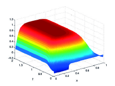
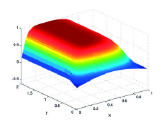
Figure 5.1: FD state $y$ for $y_{\circ}=0.1\operatorname{sgn}(x-0.3)$ (left plot) and $y_{\circ}=0.2\sin{\pi x}$ (right plot) with $u=0$, $(\theta,\rho)=(0.1,11)$ and $\mathcal{N}=99$.

As we see from Figure 5.1, the uncontrolled solutions do not tend to zero for $t\to\infty$, indeed it stabilizes at one.

5.2 POD-NMPC experiments

In our numerical examples we choose $y_{d}\equiv 0,$ i.e., we force the state to be close to zero, and $\lambda=0.01$ in (2.4). A finite horizon open loop strategy does not steer the trajectory to the zero-equilibrium (see Figure 5.2). Therefore, stabilization is not guaranteed by the theory of asymptotic stability. Note that we are not dealing with terminal constraints and the terminal condition of the adjoint equation (4.5) is zero.

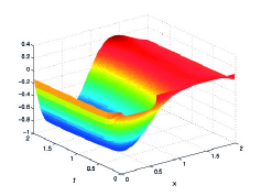
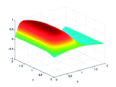
Figure 5.2: Open-loop solution $y$ for $y_{\circ}=0.1\operatorname{sgn}(x-0.3)$, $(\theta,\rho)=(0.1,11)$, $\mathcal{N}=99$, $t_{f}=2$ (left plot) and $y_{\circ}=0.2\sin{\pi x}$, $(\theta,\rho)=(0.1,11)$, $\mathcal{N}=99$, $t_{f}=2$ (right plot).

In our tests, the snapshots are computed taking the uncontrolled system, e.g. $u\equiv 0,$ in (2.1) and the correspondent adjoint equation (4.5). Several hints for the computation of the snapshots in the context of MPC are given in [14]. The nonlinear term is reduced following the Discrete Empirical Interpolation Method (DEIM) which is a method that avoid the evaluation of the full model of the nonlinear part building new basis functions upon the nonlinear term; compare [9] for more details. Note that, in our simulations, the optimal prediction horizon $N$ is always obtained from Theorem 4.6.

Run 5.1 (Unconstrained case with smooth initial data).

The parameters are presented in Table 5.1.

$T$	$\Delta t$	$\Delta x$	$\theta$	$\rho$	$y_{0}(x)$	$u_{a}$	$u_{b}$	$N$	$K$
0.5	0.01	0.01	1	11	$0.2\sin(\pi x)$	$-\infty$	$\infty$	10	2.46

Table 5.1: Run 5.1: Setting for the optimal control problem, minimal stabilizing horizon $N$ and feedback constant $K$.

According to the computation of $\alpha^{N}$ in (3.12) related to the relaxed DPP, the minimal horizon that guarantes asymptotic stability is $N=10$. Even in the POD-NMPC scheme the asymptotic stability is achieved for $N=10$, provided that $\mathsf{Err}(t;\mathfrak{l})\leq 10^{-3}$ for all $t\geq t_{\circ}$. Note that the horizon of the surrogate model is computed by (4.25). In Figure 5.3 we show the controlled state trajectory computed by Algorithm 1 taking $N=3$ and $N=10$.

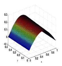
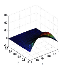
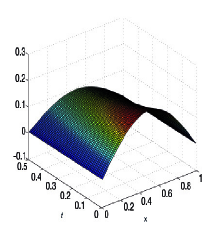
Figure 5.3: Run 5.1: NMPC state with $N=3$ (left plot), with $N=10$ (middle plot) and with $u=-Ky$ (right plot)

As we can see, we do not get a stabilizing feedback for $N=3$, whereas $N=10$ leads to a state trajectory which tends to zero for $t\to\infty$. Note that we plot the solution only on the time interval $[0,0.5]$ in order to have a zoom of the solution. Further, in Figure 5.3 the solution related to $u=-Ky$ is presented. As we can see, the NMPC control stabilized to the origin very soon while the control law $u=-Ky$ requires a larger time horizon. This is due to the fact that MPC stabilizes in an optimal way, in contrast to the control law $u=-Ky$. In Table 5.2 we present the error in $L^{2}(t_{\circ},T;H)$-norm considering the solution coming from the Algorithm 1 as the ’truth’ solution (in our case the finite difference solution denoted by $y^{FD}$). The examples are computed with $\mathsf{Err}(t,\mathfrak{l})\leq 10^{-3}.$

	$\hat{J}$	time	$K$	$\|y^{FD}-y\|_{L^{2}(t_{\circ},T;H)}$
Solution with $u=-Ky$	0.0025		2.46	0.0145
Alg. 1	0.0015	49s
Alg. 2 ($\mathfrak{l}=13,\mathfrak{l}^{DEIM}=15$)	0.0016	18s		0.0047
Alg. 2 ($\mathfrak{l}=3,\mathfrak{l}^{DEIM}=2$)	0.0016	16s		0.0058

Table 5.2: Run 5.1: Evaluation of the cost functional, CPU time, suboptimal solution.

The CPU time for the full-model turns out to be 49 seconds, whereas the POD-suboptimal approximation with only three POD and two DEIM basis functions requires 6 seconds. We can easily observe an impressive speed up factor eight. Moreover the evaluation of the cost functional in the full model and the POD model provides very close values. We have not considered the CPU time in the suboptimal problem since it did not involve a real optimazion problem. As soon as we have computed $K$, within an offline stage, we directly approximate the equation with the control law $u=-Ky$. $\Diamond$

Run 5.2 (Constrained case with smooth initial data).

In contrast to Run 5.1 we choose $u_{a}=-0.3$ and $u_{b}=0.$ As expected, the minimal horizon $N$ increases compared to Run 5.1; see Table 5.3.

$T$	$\Delta t$	$\Delta x$	$\theta$	$\rho$	$y_{0}(x)$	$u_{a}$	$u_{b}$	$N$	$K$
0.5	0.01	0.01	1	11	$0.2\sin(\pi x)$	$-0.3$	$0$	14	1.50

Table 5.3: Run 5.2: Setting for the optimal control problem, minimal stabilizing horizon $N$ and feedback constant $K$.

As one can see from Figure 5.4 the NMPC state with $N=14$ tends faster to zero than the state with $u=-Ky$.

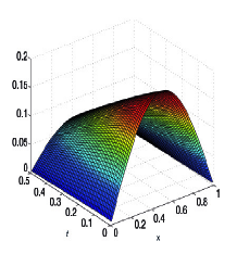
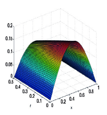
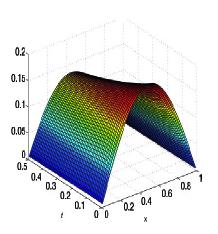
Figure 5.4: Run 5.2: NMPC state with $N=14$ (left plot), POD-NMPC state with $N=14$ (middle plot) and state with $u=-Ky$ (right plot)

The solution coming from the POD model is in the middle of Figure 5.4. Note that $\mathcal{E}(\mathfrak{l}=3)=0.01,\mathcal{E}(\mathfrak{l}=13)=0,$ and $\mathsf{Err}(t;\mathfrak{l})\leq 10^{-3}$ for any $\mathfrak{l}$ and $t\geq t_{\circ}.$ Indeed, Table 5.4 presents the evaluation of the cost functionals for the proposed algorithms and the CPU time which shows that the speed up by the reduced order approach is about 16.

	$\hat{J}$	time	$K$	$\|y^{FD}-y\|_{L^{2}(t_{\circ},T;H)}$
Solution with $u=-Ky$	0.0035		1.50	0.0089
Alg. 1	0.0027	65s
Alg. 2 ($\mathfrak{l}=13$, $\mathfrak{l}^{DEIM}=15$)	0.0032	15s		0.0054
Alg. 2 ($\mathfrak{l}=3$, $\mathfrak{l}^{DEIM}=2$)	0.0033	14s		0.0055

Table 5.4: Run 5.2: Evaluation of the cost functional, CPU times, suboptimal solution.

Note that $K$ in Run 5.2 is smaller compared to Run 5.1 due to the constraint of the control space. Further, the error is presented in Table 5.4. To study the influence of $\mathsf{Err}(t;\mathfrak{l})$ we present in Figure 5.5, on the left, how the optimal prediction horizon $N$ changes according to different tolerance.

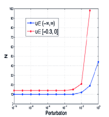
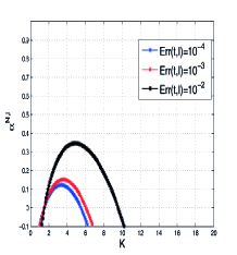
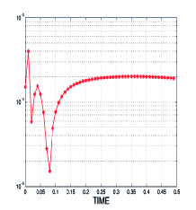
Figure 5.5: Run 5.2: Optimal horizon $N$ and $\alpha^{N,\mathfrak{l}}$ according to different $\mathsf{Err}(t;\mathfrak{l})=10^{-3}$, Influence of the relative error $t\mapsto\mathsf{Err}(t;\mathfrak{l})=10^{-3}$ for $\mathfrak{l}=3$.

The blue line corresponds to the optimal prediction horizon in Run 5.1, and the red one to Run 5.2. It turns out that, as long as $\mathsf{Err}(t;\mathfrak{l})\leq 10^{-3},$ we can work exactly with the same horizon $N$ we had in the full model in both examples. In the middle plot of Figure 5.5 there is a zoom of the function $\alpha$ with different values of $\mathsf{Err}(t;\mathfrak{l})$ with respect to Run 5.2. The right plot of Figure 5.5 shows the relative error $\mathsf{Err}(t;\mathfrak{l})$ for $0\leq t\leq 0.5$ with $\mathfrak{l}=3$. One of the big advantages of feedback control is the stabilization under perturbation of the system. The perturbation of the initial condition is a typical example which comes from many applications in fact, often the measurements may not be correct. For a given noise distribution $\delta=\delta(x)$ we consider a perturbation the following form:

$$y_{0}(x)=\big{(}1+\delta(x)\big{)}y_{\circ}(x)\quad\text{for }x\in\Omega.$$

The perturbation is applied only at every initial condition of the MPC algorithm (see ($\mathbf{P^{\boldsymbol{N}}(}t_{\circ}\mathbf{)}$) in Algorithm 1) and it is random with respect to the spatial variable. The study of the asympotic stability does not change: we can compute the minimal prediction horizon as before. As we can see in Figure 5.6 the POD-NMPC algorithm is able to stabilize with a noise of $|\delta(x)|\leq 30\%$. $\Diamond$

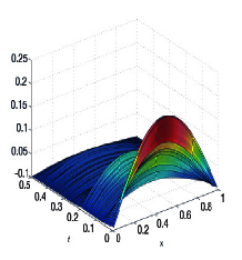
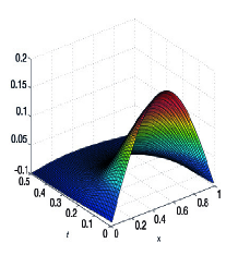
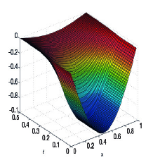
Figure 5.6: Run 5.2: POD-NMPC state with $30\%$ noise (left plot); Run 5.3: NMPC state with $N=30$ (middle plot) and POD-NMPC state with $N=30$, $\mathfrak{l}=\mathfrak{l}^{DEIM}=16$ (right plot).

Run 5.3 (Constrained case with smooth initial data).

Now we decrease the diffusion term and, as a consequence, the prediction horizon $N$ increases; see Table 5.5 and middle plot of Figure 5.6.

$T$	$\Delta t$	$\Delta x$	$\theta$	$\rho$	$y_{0}(x)$	$u_{a}$	$u_{b}$	$N$	$K$
0.5	0.01	0.01	$1/\sqrt{2}$	10	$0.2\sin(\pi x)$	$-1$	$0$	30	5

Table 5.5: Run 5.3: Setting for the optimal control problem.

Even if the horizon is very large, the proposed Algorithm 2 accelerates the approximation of the problem. The decrease of $\theta$ may give some troubles with the POD-model since the domination of the convection term causes a high-variability in the solution, then a few basis functions will not suffice to obtain good surrogate models (see [1, 2]). Note that, in our example, the diffusion term is still relevant such that we can work with only 2 POD basis functions. The CPU time in the full model is $84$ seconds, whereas with a low-rank model, such as $\mathfrak{l}=2$ we obtained the solution in five seconds and an impressive speed up factor of 16. Even with a more accurate POD model we have a very good speed up factor of nine. The evaluation of the cost functional is given in Table 5.6.

	$\hat{J}$	time	$K$	$\|y^{FD}-y\|_{L^{2}(t_{\circ},T;H)}$
Suboptimal solution ($u=-Ky$)	0.0021		5	0.0208
Algorithm 1	0.0016	84s
Algorithm 2 ($\mathfrak{l}=16$, $\mathfrak{l}^{DEIM}=16$)	0.0017	19s		0.0092
Algorithm 2 ($\mathfrak{l}=2$, $\mathfrak{l}^{DEIM}=3$)	0.0018	15s		0.0093

Table 5.6: Run 5.3: Evaluation of the cost functional and CPU time.

In the right plot of Figure 5.6 the POD-NMPC state is plotted for $\mathfrak{l}=16$ POD basis and $\mathfrak{l}^{DEIM}=16$ DEIM ansatz functions. The error between the NMPC state and the POD-MPC state is less than 0.01 . $\Diamond$

Run 5.4 (Constrained case with no-smooth initial data).

In the last test we focus on a different initial condition and different control constraints. The parameters are presented in Table 5.7.

$T$	$\Delta t$	$\Delta x$	$\theta$	$\rho$	$y_{0}(x)$	$u_{a}$	$u_{b}$	$N$	$K$
0.5	0.01	0.01	1/2	5	$0.1\operatorname{sgn}(x-0.3)$	-1	1	43	9.99

Table 5.7: Run 5.4: Setting for the optimal control problem.

The minimal horizon $N$ which ensures asymptotic stability is $N=43$. Table 5.8 emphazises again the performance of the POD-NMPC method with an acceleration 12 times faster than the full model.

	$\hat{J}$	time	$K$	$\|y^{FD}-y\|_{L^{2}(t_{\circ},T;H)}$
Solution with $u=-Ky$	4.7e-4		9.99	0.0060
Alg. 1	4.1e-4	50s
Alg. 2 ($\mathfrak{l}=17$, $\mathfrak{l}^{DEIM}=19$)	4.4e-4	12s		0.0034
Alg. 2 ($\mathfrak{l}=3$, $\mathfrak{l}^{DEIM}=4$)	4.4e-4	14s		0.0035

Table 5.8: Run 5.4: Cost functional, CPU time and suboptimal solution.

The evaluation of the cost functional gives the same order in all the simulation we provide. In Figure 5.7 we present the NMPC state for $N=43$ (left plot), the POD-NMPC state with $N=43$, $\mathfrak{l}=3$, $\mathfrak{l}^{DEIM}=4$ (middle plot) and the increase of the optimal horizon $N$ according to the perturbation $\mathsf{Err}(t;\mathfrak{l})$.

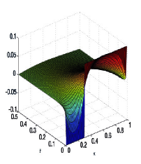
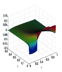
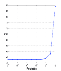
Figure 5.7: Run 5.4: NMPC state with $N=43$ (left plot), POD-NMPC state with $N=43,$ $\mathfrak{l}=17$, $\mathfrak{l}^{DEIM}=19$ (middle plot) and increase of the optimal horizon $N$ according to the perturbation $\mathsf{Err}(t;\mathfrak{l})$ (right plot).

The error between the NMPC state and the POD-MPC state is 0.0035 when $\mathcal{E}(\mathfrak{l}=3)=0.01,$ whereas for $\mathcal{E}(\mathfrak{l}=17)=0$ the error is 0.0034. $\Diamond$

6 Conclusions

We have proposed a new numerical method for optimal control problems which tries to stabilize a one dimensional semilinear parabolic equation by means of Nonlinear MPC. We presented asymptotic stability conditions, where the control space is bounded for a suboptimal problem coming from a particular class of feedback controls.
Since the CPU time of the full dimensional algorithm may increase with the dimension of the prediction horizon, we have presented a deep study of the suboptimal model which comes from POD model reduction. We have given an a-priori error estimate for the computation of the prediction horizon of the suboptimal model. The new reduced model approach turns out to be computationally very efficient with respect to the full dimensional problem. If the approximation quality (4.23) of the reduced-order model is taken into account, stabilization is also guaranteed by our theory. Although the algorithm is applied to a one dimensional problem, the theory is rather general and can be applied to higher dimensional equations, not only with POD model reduction but any (reduced-order) method provided the error term in (4.23) is small for reasonable small $\mathfrak{l}$.

Appendix A Proof of Lemma 3.6

Choosing $u(t)=-Ky(t)$, $\varphi=y(t)$ in (2.3) and using $\int_{\Omega}y(t)^{4}\,\mathrm{d}x\geq 0$, $\int_{\Omega}y_{x}(t)y(t)\,\mathrm{d}x=0$ f.a.a. $t\geq t_{\circ}$ we find

$$\frac{1}{2}\frac{\mathrm{d}}{\mathrm{d}t}\,{\|y(t)\|}^{2}_{H}+\theta\,{\|y(t)\|}_{V}^{2}+(K-\rho)\,{\|y(t)\|}_{H}^{2}\leq 0\quad\text{f.a.a. }t\geq t_{\circ}$$

Hence, (3.8) imply

$$\frac{\mathrm{d}}{\mathrm{d}t}\,{\|y(t)\|}^{2}_{H}\leq-2\bigg{(}\frac{\theta}{C_{V}}+K-\rho\bigg{)}\,{\|y(t)\|}_{H}^{2}=-2\gamma(K)\,{\|y(t)\|}_{H}^{2}\quad\text{f.a.a. }t\geq t_{\circ}.$$

Thus, by Gronwall’s inequality we derive

$${\|y(t)\|}^{2}_{H}\leq e^{-2\gamma(K)(t-t_{\circ})}\,{\|y_{\circ}\|}_{H}^{2}\quad\text{f.a.a. }t\geq t_{\circ}.$$

which gives (3.9). $\Box$

Appendix B Proof of Theorem 4.5

Recall that $H^{\mathfrak{l}}\subset V$ holds. Consequently, $\|\psi_{i}^{H}-\mathcal{P}^{\mathfrak{l}}_{H}\psi_{i}^{H}\|_{V}$ is well-defined for $1\leq i\leq\mathfrak{l}$. First we review a result from [27, Theorem 6.2], which is essential in our proof of Theorem 4.5 for the choice $X=H$: Suppose that $y^{k}\in L^{2}(t_{\circ},t_{\circ}^{N};V)$ for $1\leq k\leq\wp$. Then,

$$\sum_{k=1}^{\wp}\int_{t_{\circ}}^{t_{\circ}^{N}}{\|y^{k}(t)-\mathcal{P}_{H}^{\mathfrak{l}}y^{k}(t)\|}_{V}^{2}\,\mathrm{d}t=\sum_{i=\mathfrak{l}+1}^{d}\lambda_{i}^{H}\,{\|\psi_{i}^{H}-\mathcal{P}^{\mathfrak{l}}_{H}\psi_{i}^{H}\|}_{V}^{2}.$$ (2.1)

Moreover, $\mathcal{P}^{\mathfrak{l}}_{H}y^{k}$ converges to $y^{k}$ in $L^{2}(0,T;V)$ as $\mathfrak{l}$ tends to $\infty$ for each $k\in\{1,\ldots,\wp\}$.

Proof of Theorem 4.5. To derive an error estimate for $\|y-y^{\mathfrak{l}}\|_{\mathbb{Y}^{N}(t_{\circ})}$ we make use of the decomposition

$$y(t)-y^{\mathfrak{l}}(t)=y(t)-\mathcal{P}^{\mathfrak{l}}y(t)+\mathcal{P}^{\mathfrak{l}}y(t)-y^{\mathfrak{l}}(t)=\varrho^{\mathfrak{l}}(t)+\vartheta^{\mathfrak{l}}(t)\text{ f.a.a. }t\in[t_{\circ},t_{\circ}^{N}]$$

with $\varrho^{\mathfrak{l}}(t)=y(t)-\mathcal{P}^{\mathfrak{l}}y(t)\in(X^{\mathfrak{l}})^{\bot}$ and $\vartheta^{\mathfrak{l}}(t)=\mathcal{P}^{\mathfrak{l}}y(t)-y^{\mathfrak{l}}(t)\in X^{\mathfrak{l}}$. Recall that $\mathbb{Y}^{N}(t_{\circ})=W(t_{\circ},t_{\circ}^{N})$ holds. Since $\varrho_{t}^{\mathfrak{l}}(t)\in V$ holds f.a.a. $t\in[t_{\circ},t_{\circ}^{N}]$, we have $\|\varrho_{t}^{\mathfrak{l}}(t)\|_{V^{\prime}}=\|\varrho_{t}^{\mathfrak{l}}(t)\|_{V}$ due to the Riesz theorem [25, p. 43]. Hence it follows from (4.15) and (2.1) that

$${\|\varrho^{\mathfrak{l}}\|}_{\mathbb{Y}^{N}(t_{\circ})}^{2} =\int_{t_{\circ}}^{t_{\circ}^{N}}{\|\varrho^{\mathfrak{l}}(t)\|}_{V}^{2}+{\|\varrho^{\mathfrak{l}}_{t}(t)\|}_{V}^{2}\,\mathrm{d}t$$ (2.2)

$$=\left\{\begin{aligned} &\sum_{i=\mathfrak{l}+1}^{d}\lambda_{i}^{V}&&\text{for }X=V,\\ &\sum_{i=\mathfrak{l}+1}^{d}\lambda_{i}^{H}{\|\psi_{i}^{H}-\mathcal{P}_{H}^{\mathfrak{l}}\psi_{i}^{H}\|}_{V}^{2}&&\text{for }X=H.\end{aligned}\right.$$

Next we estimate $\vartheta^{\mathfrak{l}}(t)$. We infer from $\vartheta^{\mathfrak{l}}(t)=\mathcal{P}^{\mathfrak{l}}y(t)-y^{\mathfrak{l}}(t)$ that

$${\langle\vartheta^{\mathfrak{l}}_{t}(t),\psi\rangle}_{V^{\prime},V}+{\langle\theta\vartheta^{\mathfrak{l}}(t),\psi\rangle}_{V}$$ (2.3)

$$\quad={\langle y_{t}(t)-y^{\mathfrak{l}}_{t}(t)+\mathcal{P}^{\mathfrak{l}}y(t)-y^{\mathfrak{l}}(t),\psi\rangle}_{V^{\prime},V}+\theta\,{\langle\mathcal{P}^{\mathfrak{l}}y(t)-y^{\mathfrak{l}}(t),\psi\rangle}_{V}$$

for all $\psi\in X^{\mathfrak{l}}$ and f.a.a. $t\in[t_{\circ},t_{\circ}^{N}]$. For $X=V$ we have

$${\langle\mathcal{P}^{\mathfrak{l}}_{V}y(t),\psi\rangle}_{V}={\langle y(t),\psi\rangle}_{V}\quad\text{for all }\psi\in X^{\mathfrak{l}}\text{ and f.a.a. }t\in[t_{\circ},t_{\circ}^{N}].$$

Hence, we derive from (2.3), (4.2) and (4.16) that

$${\langle\vartheta^{\mathfrak{l}}_{t}(t),\psi\rangle}_{V^{\prime},V}+{\langle\theta\vartheta^{\mathfrak{l}}(t),\psi\rangle}_{V}$$ (2.4)

$$\quad={\langle\rho(y(t)-y^{\mathfrak{l}}(t))-\rho(y(t)^{3}-y^{\mathfrak{l}}(t)^{3}),\psi\rangle}_{H}+{\langle\mathcal{P}^{\mathfrak{l}}_{V}y_{t}(t)-y_{t}(t),\psi\rangle}_{V^{\prime},V}$$

for all $\psi\in V^{\mathfrak{l}}$ and f.a.a. $t\in[t_{\circ},t_{\circ}^{N}]$. For $s\in[0,1]$ we define the function $\xi^{\mathfrak{l}}(s)=y^{\mathfrak{l}}+s(y-y^{\mathfrak{l}})$. Then it follows from (4.3) and (4.17) that

$${\|\xi^{\mathfrak{l}}(s)\|}_{L^{\infty}(Q^{N})}\leq s\,{\|y\|}_{L^{\infty}(Q^{N})}+(1-s)\,{\|y^{\mathfrak{l}}\|}_{L^{\infty}(Q^{N})}\leq C_{1}\quad\text{for all }s\in[0,1]$$

with a constant $C_{1}>0$ dependent on $y_{\circ}$, $u_{a}$ and $u_{b}$, but independent of $y$, $y^{\mathfrak{l}}$ and $\mathfrak{l}$. By the mean value theorem we obtain

$${\langle y(t)^{3}-y^{\mathfrak{l}}(t)^{3},\psi\rangle}_{H} =\bigg{\langle}\frac{1}{4}\int_{0}^{1}\xi^{\mathfrak{l}}(s;t)^{4}\big{(}y(t)-y^{\mathfrak{l}}(t)\big{)}\,\mathrm{d}s,\psi\bigg{\rangle}_{H}$$

$$\leq C_{2}\,{\|y(t)-y^{\mathfrak{l}}(t)\|}_{H}{\|\psi\|}_{H}\quad\text{for all }\psi\in V^{\mathfrak{l}}$$

with $C_{2}=C_{1}^{4}/4$. We set $C_{3}=\rho(1+C_{2})$. Hence, choosing $\psi=\vartheta^{\mathfrak{l}}(t)\in V^{\mathfrak{l}}$ and utilizing $\theta\geq\theta_{a}>0$ we obtain from $y(t)-y^{\mathfrak{l}}(t)=\varrho^{\mathfrak{l}}(t)+\vartheta^{\mathfrak{l}}(t)$, (2.4), (3.8) and Young’s inequality

$$\frac{1}{2}\frac{\mathrm{d}}{\mathrm{d}t}\,{\|\vartheta^{\mathfrak{l}}(t)\|}_{H}^{2}+\theta_{a}\,{\|\vartheta^{\mathfrak{l}}(t)\|}_{V}^{2}$$

$$\leq C_{3}\,{\|y(t)-y^{\mathfrak{l}}(t)\|}_{H}{\|\vartheta^{\mathfrak{l}}(t)\|}_{H}+{\|\mathcal{P}^{\mathfrak{l}}_{V}y_{t}(t)-y_{t}(t)\|}_{V^{\prime}}{\|\vartheta^{\mathfrak{l}}(t)\|}_{V}$$

$$\leq C_{3}\,\bigg{(}\frac{C_{V}^{2}}{2}\,{\|\varrho^{\mathfrak{l}}(t)\|}_{V}^{2}+\frac{3}{2}\,{\|\vartheta^{\mathfrak{l}}(t)\|}_{H}^{2}\bigg{)}+\frac{1}{2\theta_{a}}{\|\varrho^{\mathfrak{l}}_{t}(t)\|}_{V^{\prime}}^{2}+\frac{\theta_{a}}{2}\,{\|\vartheta^{\mathfrak{l}}(t)\|}_{V}^{2}$$

$$\leq\frac{C_{4}}{2}\,\big{(}{\|\varrho^{\mathfrak{l}}(t)\|}_{V}^{2}+{\|\varrho^{\mathfrak{l}}_{t}(t)\|}_{V}^{2}\big{)}+\frac{3C_{3}}{2}\,{\|\vartheta^{\mathfrak{l}}(t)\|}_{H}^{2}+\frac{\theta_{a}}{2}\,{\|\vartheta^{\mathfrak{l}}(t)\|}_{V}^{2}$$

f.a.a. $t\in[t_{\circ},t_{\circ}^{N}]$ with the constant $C_{4}=\max(C_{3}C_{V}^{2},1/\theta_{a})$. Hence, we have

$$\frac{\mathrm{d}}{\mathrm{d}t}\,{\|\vartheta^{\mathfrak{l}}(t)\|}_{H}^{2}+\theta_{a}\,{\|\vartheta^{\mathfrak{l}}(t)\|}_{V}^{2}\leq C_{5}\,\big{(}{\|\varrho^{\mathfrak{l}}(t)\|}_{V}^{2}+{\|\varrho^{\mathfrak{l}}_{t}(t)\|}_{V}^{2}+{\|\vartheta^{\mathfrak{l}}(t)\|}_{H}^{2}\big{)}$$ (2.5)

for $C_{5}=\max(C_{4},3C_{3})$ and f.a.a. $t\in[t_{\circ},t_{\circ}^{N}]$. By Gronwall’s inequality and (2.2) we derive from (2.5)

$${\|\vartheta^{\mathfrak{l}}(t)\|}_{H}^{2} \leq e^{C_{5}(t-t_{\circ})}\bigg{(}{\|\vartheta^{\mathfrak{l}}(t_{\circ})\|}_{H}^{2}+\int_{t_{\circ}}^{t_{\circ}^{N}}{\|\varrho^{\mathfrak{l}}(s)\|}_{V}^{2}+{\|\varrho^{\mathfrak{l}}_{t}(s)\|}_{V}^{2}\,\mathrm{d}s\bigg{)}$$ (2.6)

$$\leq C_{6}\bigg{(}{\|\vartheta^{\mathfrak{l}}(t_{\circ})\|}_{H}^{2}+\sum_{i=\mathfrak{l}+1}^{\infty}\lambda_{i}^{V}\bigg{)}\quad\text{f.a.a. }t\in[t_{\circ},t_{\circ}^{N}]$$

f.a.a. $t\in[t_{\circ},t_{\circ}^{N}]$ with $C_{6}=e^{C_{5}(t_{\circ}^{N}-t_{\circ})}$. Now we turn to the case $X=H$. We have

$${\langle\mathcal{P}^{\mathfrak{l}}_{H}y(t),\psi\rangle}_{V}={\langle y(t),\psi\rangle}_{V}+{\langle\mathcal{P}^{\mathfrak{l}}_{H}y(t)-y(t),\psi\rangle}_{V}$$

so that (2.3), (4.2) and (4.16) that

$${\langle\vartheta^{\mathfrak{l}}_{t}(t),\psi\rangle}_{V^{\prime},V}+{\langle\theta\vartheta^{\mathfrak{l}}(t),\psi\rangle}_{V}={\langle\rho(y(t)-y^{\mathfrak{l}}(t))-\rho(y(t)^{3}-y^{\mathfrak{l}}(t)^{3}),\psi\rangle}_{H}$$ (2.7)

$$\hskip 85.35826pt+{\langle\mathcal{P}^{\mathfrak{l}}_{H}y(t)-y(t),\psi\rangle}_{V}+{\langle\mathcal{P}^{\mathfrak{l}}_{V}y_{t}(t)-y_{t}(t),\psi\rangle}_{V^{\prime},V}$$

for all $\psi\in H^{\mathfrak{l}}$ and f.a.a. $t\in[t_{\circ},t_{\circ}^{N}]$. Now we proceed analogously as in the case $X=V$ and obtain

$$\frac{1}{2}\frac{\mathrm{d}}{\mathrm{d}t}\,{\|\vartheta^{\mathfrak{l}}(t)\|}_{H}^{2}+\theta_{a}\,{\|\vartheta^{\mathfrak{l}}(t)\|}_{V}^{2}$$

$$\leq\frac{C_{7}}{2}\,\big{(}{\|\varrho^{\mathfrak{l}}(t)\|}_{V}^{2}+{\|\varrho^{\mathfrak{l}}_{t}(t)\|}_{V}^{2}+{\|\vartheta^{\mathfrak{l}}(t)\|}_{H}^{2}\big{)}+\frac{\theta_{a}}{2}\,{\|\vartheta^{\mathfrak{l}}(t)\|}_{V}^{2}$$

f.a.a. $t\in[t_{\circ},t_{\circ}^{N}]$ with the constant $C_{7}=\max(C_{3}C_{V}^{2}+2/\theta_{a},2C_{3})$. Therefore, we derive

$$\frac{\mathrm{d}}{\mathrm{d}t}\,{\|\vartheta^{\mathfrak{l}}(t)\|}_{H}^{2}+\theta_{a}\,{\|\vartheta^{\mathfrak{l}}(t)\|}_{V}^{2}\leq C_{7}\,\big{(}{\|\varrho^{\mathfrak{l}}(t)\|}_{V}^{2}+{\|\varrho^{\mathfrak{l}}_{t}(t)\|}_{V}^{2}+{\|\vartheta^{\mathfrak{l}}(t)\|}_{H}^{2}\big{)};$$ (2.8)

compare (2.5). Utilizing Gronwall’s inequality and (2.2) we infer – instead of (2.6) – that

$${\|\vartheta^{\mathfrak{l}}(t)\|}_{H}^{2}\leq C_{8}\bigg{(}{\|\vartheta^{\mathfrak{l}}(t_{\circ})\|}_{H}^{2}+\sum_{i=\mathfrak{l}+1}^{\infty}\lambda_{i}^{H}\,{\|\psi_{i}^{H}-\mathcal{P}_{H}^{\mathfrak{l}}\psi_{i}^{H}\|}_{V}^{2}\bigg{)}$$ (2.9)

f.a.a. $t\in[t_{\circ},t_{\circ}^{N}]$ with $C_{8}=e^{C_{7}(t_{\circ}^{N}-t_{\circ})}$. We summarize (2.6) and (2.8) in

$${\|\vartheta^{\mathfrak{l}}(t)\|}_{H}^{2}\leq C_{9}\cdot\left\{\begin{aligned} &{\|\vartheta^{\mathfrak{l}}(t_{\circ})\|}_{H}^{2}+\sum_{i=\mathfrak{l}+1}^{d}\lambda_{i}^{V}&&\text{for }X=V,\\ &{\|\vartheta^{\mathfrak{l}}(t_{\circ})\|}_{H}^{2}+\sum_{i=\mathfrak{l}+1}^{d}\lambda_{i}^{H}{\|\psi_{i}^{H}-\mathcal{P}_{H}^{\mathfrak{l}}\psi_{i}^{H}\|}_{V}^{2}&&\text{for }X=H\end{aligned}\right.$$ (2.10)

f.a.a. $t\in[t_{\circ},t_{\circ}^{N}]$ with $C_{9}=\max(C_{6},C_{8})$. Furthermore, (2.5) and (2.8), respectively, imply by integration over $[t_{\circ},t_{\circ}^{N}]$

$${\|\vartheta^{\mathfrak{l}}\|}_{L^{2}(t_{\circ},t_{\circ}^{N};V)}^{2}\leq\frac{1}{\theta_{a}}\,{\|\vartheta^{\mathfrak{l}}(t_{\circ})\|}_{H}^{2}+\frac{C_{10}}{\theta_{a}}\,\big{(}{\|\varrho^{\mathfrak{l}}\|}_{W(t_{\circ},t_{\circ}^{N})}^{2}+{\|\vartheta^{\mathfrak{l}}\|}_{L^{2}(t_{\circ},t_{\circ}^{N};H)}^{2}\big{)}$$ (2.11)

$$\quad\leq C_{11}\cdot\left\{\begin{aligned} &{\|\vartheta^{\mathfrak{l}}(t_{\circ})\|}_{H}^{2}+\sum_{i=\mathfrak{l}+1}^{d}\lambda_{i}^{V}&&\text{for }X=V,\\ &{\|\vartheta^{\mathfrak{l}}(t_{\circ})\|}_{H}^{2}+\sum_{i=\mathfrak{l}+1}^{d}\lambda_{i}^{H}{\|\psi_{i}^{H}-\mathcal{P}_{H}^{\mathfrak{l}}\psi_{i}^{H}\|}_{V}^{2}&&\text{for }X=H\end{aligned}\right.$$

with $C_{10}=\max(C_{5},C_{7})$ and $C_{11}=C_{10}\max(1,(t_{\circ}^{N}-t_{\circ})\max(C_{6},C_{8}))/\theta_{a}$. From estimates (2.10), (2.11), from

$$y(t)^{3}-y^{\mathfrak{l}}(t)^{3}=\big{(}\varrho^{\mathfrak{l}}(t)+\vartheta^{\mathfrak{l}}(t)\big{)}\big{(}y(t)^{2}+y(t)y^{\mathfrak{l}}(t)+y^{\mathfrak{l}}(t)^{2}\big{)}\quad\text{f.a.a. }t\in[t_{\circ},t_{\circ}^{N}]$$

and from the embedding inequalities [11]

$${\|\varphi\|}_{L^{\infty}(\Omega)} \leq C_{\infty}\,{\|\varphi\|}_{V} \text{for all }\varphi\in V,$$

$${\|\varphi\|}_{C([t_{\circ},t_{\circ}^{N}];H)} \leq C_{W}\,{\|\varphi\|}_{W(t_{\circ},t_{\circ}^{N})} \text{for all }\varphi\in W(t_{\circ},t_{\circ}^{N})$$ (2.12)

for two constants $C_{\infty},\,C_{W}>0$ we infer that

$${\|\vartheta^{\mathfrak{l}}\|}_{L^{2}(t_{\circ},t_{\circ}^{N};V^{\prime})}=\sup_{{\|\varphi\|}_{L^{2}(t_{\circ},t_{\circ}^{N};V)}=1}\int_{t_{\circ}}^{t_{\circ}^{N}}{\langle\vartheta^{\mathfrak{l}}(t),\varphi(t)\rangle}_{V^{\prime},V}\,\mathrm{d}t$$

$$\quad\leq\sup_{{\|\varphi\|}_{L^{2}(t_{\circ},t_{\circ}^{N};V)}=1}\int_{t_{\circ}}^{t_{\circ}^{N}}{\langle\rho(y(t)-y^{\mathfrak{l}}(t)),\varphi(t)\rangle}_{H}+{\langle\rho(y(t)^{3}-y^{\mathfrak{l}}(t)^{3}),\varphi(t)\rangle}_{H}\,\mathrm{d}t$$

$$\qquad+\sup_{{\|\varphi\|}_{L^{2}(t_{\circ},t_{\circ}^{N};V)}=1}\int_{t_{\circ}}^{t_{\circ}^{N}}{\langle\mathcal{P}^{\mathfrak{l}}y_{t}(t)-y_{t}(t),\varphi(t)\rangle}_{V^{\prime},V}-{\langle\theta\vartheta^{\mathfrak{l}}(t),\varphi(t)\rangle}_{V}\,\mathrm{d}t$$

$$\quad\leq\rho C_{V}\big{(}{\|\varrho^{\mathfrak{l}}\|}_{L^{2}(t_{\circ},t_{\circ}^{N};H)}+{\|\vartheta^{\mathfrak{l}}\|}_{L^{2}(t_{\circ},t_{\circ}^{N};H)}\big{)}+\theta\,{\|\vartheta^{\mathfrak{l}}\|}_{L^{2}(t_{\circ},t_{\circ}^{N};V)}$$

$$\qquad+C_{7}\,\big{(}{\|\varrho^{\mathfrak{l}}\|}_{L^{\infty}(t_{\circ},t_{\circ}^{N};H)}+{\|\vartheta^{\mathfrak{l}}\|}_{L^{\infty}(t_{\circ},t_{\circ}^{N};H)}\big{)}+{\|\varrho_{t}^{\mathfrak{l}}\|}_{L^{2}(t_{\circ},t_{\circ}^{N};V^{\prime})}$$

where $C_{7}>0$ satisfies $C_{\infty}\,\|y^{2}+yy^{\mathfrak{l}}+(y^{\mathfrak{l}})^{2}\|_{L^{2}(t_{\circ},t_{\circ}^{N};H)}\leq C_{7}$. Hence, there is a constant $C_{8}>0$ depending on $\theta$, $\rho$, $C_{W}$, $C_{9}$, $C_{11}$ such that

$${\|\vartheta^{\mathfrak{l}}\|}_{L^{2}(t_{\circ},t_{\circ}^{N};V^{\prime})}^{2}$$ (2.13)

$$\quad\leq C_{8}\cdot\left\{\begin{aligned} &{\|\vartheta^{\mathfrak{l}}(t_{\circ})\|}_{H}^{2}+\sum_{i=\mathfrak{l}+1}^{d}\lambda_{i}^{V}&&\text{for }X=V,\\ &{\|\vartheta^{\mathfrak{l}}(t_{\circ})\|}_{H}^{2}+\sum_{i=\mathfrak{l}+1}^{d}\lambda_{i}^{H}{\|\psi_{i}^{H}-\mathcal{P}_{H}^{\mathfrak{l}}\psi_{i}^{H}\|}_{V}^{2}&&\text{for }X=H.\end{aligned}\right.$$

Form (2.10), (2.11) and (2.13) we infer the a-priori error estimate of Theorem 4.5, which motivates the use of a POD approximation for our state equation (4.2). $\Box$

References

- [1] A. Alla and M. Falcone. An adaptive POD approximation method for the control of advection-diffusion equations. In Control and Optimization with PDE Constraints, K. Kunisch, K. Bredies, C. Clason, G. von Winckel (eds), International Series of Numerical Mathematics, Vol. 164, Birkhäuser, Basel, pp 1-17, 2013.
- [2] A. Alla and M. Falcone. A Time-Adaptive POD Method for Optimal Control Problems. Proceedings of the 1st IFAC Workshop on Control of Systems Modeled by Partial Differential Equations, pp. 245-250, 2013.
- [3] F. Allgöwer, R. Findeisen, and Z.K. Nagy. Nonlinear model predictive control: from theory to application. J. Chin. Inst. Chem. Engrs., 35:299-315, 2004.
- [4] F. Allgöwer and H. Chen. A quasi-infinite horizon nonlinear model predictive control scheme with guaranteed stability. Automatica, 34:1205-1217, 1998.
- [5] N. Altmüller and L. Grüne. A comparative stability analysis of Neumann and Dirichlet boundary MPC for the heat equation. Proceedings of the 1st IFAC Workshop on Control of Systems Modeled by Partial Differential Equations, pp. 1161-1166, 2013.
- [6] N. Altmüller, L. Grüne, and K. Worthmann. Receding horizon optimal control for the wave equation. Proceedings of the 49th IEEE Conference on Decision and Control, Atlanta, Georgia, 3427 - 3432, 2010.
- [7] M. Bardi and I. Capuzzo-Dolcetta. Optimal Control and Viscosity Solutions of Hamilton-Jacobi-Bellman Equations. Birkhäuser, Basel, 1997.
- [8] T. Cazenave and A. Haraux. An Introduction to Semilinear Evolution Equation. Oxford Science Publications, 1998.
- [9] S. Chaturantabut and D.C. Sorensen. Discrete Empirical Interpolation for NonLinear Model Reduction. SIAM J. Sci. Comput., 32:2737-2764, 2010.
- [10] R. Dautray and J.-L. Lions. Mathematical Analysis and Numerical Methods for Science and Technology. Volume 5: Evolution Problems I. Springer, Berlin, 2000.
- [11] L.C. Evans. Partial Differential Equations. American Math. Society, Providence, Rhode Island, 2008.
- [12] R. Findeisen and F. Allgöwer. An introduction to nonlinear model predictive control. In C.W. Scherer and J.M. Schumacher, editors, Summerschool on The Impact of Optimization in Control. Dutch Institute of Systems and Control, DISC, 2001.
- [13] R. Findeisen and F. Allgöwer. The quasi-infinte horizon approach to nonlinear model predictive control. In A. Zinober and D. Owens, editors, Nonlinear and Adaptive Control, Lecture Notes in Control and Information Sciences. Springer-Verlag, Berlin, 89-105, 2002.
- [14] J. Ghiglieri and S. Ulbrich Optimal Flow Control Based on POD and MPC and an Application to the Cancellation of Tollmien-Schlichting Waves. Submitted, 2012.
- [15] L. Grüne and J. Pannek. Nonlinear Model Predictive Control. Springer London, 2011.
- [16] L. Grüne, J. Panneck, M. Seehafer, and K. Worthmann. Analysis of unconstrained nonlinear MPC schemes with time varying control horizon. SIAM Journal on Control and Optimization, 48:4938 - 4962, 2010.
-
[17]
M. Gubisch and S. Volkwein.
Proper Orthogonal Decomposition for Linear-Quadratic Optimal Control.
Submitted, 2013.
http://kops.ub.uni-konstanz.de/handle/urn:nbn:de:bsz:352-250378 - [18] P. Holmes, J.L. Lumley, G. Berkooz, and C.W. Romley. Turbulence, Coherent Structures, Dynamical Systems and Symmetry. Cambridge Monographs on Mechanics, Cambridge University Press, 2nd edition, 2012.
- [19] K. Ito and K. Kunisch. Receding horizon control for infinite dimensional systems. ESAIM, Control, Optimization and Calculus of Variations, 8:741-760, 2002.
- [20] K. Kunisch and S. Volkwein. Galerkin proper orthogonal decomposition methods for parabolic problems. Numerische Mathematik, 90:117-148, 2001.
- [21] K. Kunisch and S. Volkwein. Galerkin proper orthogonal decomposition methods for a general equation in fluid dynamics. SIAM Journal on Numerical Analysis, 40:492-515, 2002.
- [22] K. Kunisch and S. Volkwein, and L. Xie. HJB-POD based feedback design for the optimal control of evolution problems. SIAM Journal on Applied Dynamical Systems, 3:701-722, 2004.
- [23] G. Pannocchia, J.B. Rawlings, and S.J. Wright. Conditions under which suboptimal nonlinear MPC is inherently robust. In 18th IFAC World Congress, Milan, Italy, Sep. 2011.
- [24] J.B. Rawlings and D.Q. Mayne. Model Predictive Control: Theory and Design. Nob Hill Publishing, LLC, 2009.
- [25] M. Reed and B. Simon. Methods of Modern Mathematical Physics I: Functional Analysis. Academic Press, New York, 1980.
- [26] E.W. Sachs and M. Schu. A-priori error estimates for reduced order models in finance. ESAIM: Mathematical Modelling and Numerical Analysis, 47:449-469, 2013.
- [27] J.R. Singler. New POD expressions, error bounds, and asymptotic results for reduced order models of parabolic PDEs. Submitted, 2013.
- [28] L. Sirovich. Turbulence and the dynamics of coherent structures. Parts I-II. Quarterly of Applied Mathematics, XVL:561-590, 1987.
- [29] F. Tröltzsch. Optimal Control of Partial Differential Equations: Theory, Methods and applications. Graduate Studies in Mathematics, Vol. 112, American Mathematical Society, 2010.
- [30] S. Volkwein. Lagrange-SQP techniques for the control constrained optimal boundary control for the Burgers equation. Computational Optimization and Applications, 26:253:284, 2003.