Dynamic Complexity of Planar 3-connected Graph Isomorphism

Abstract

Dynamic Complexity (as introduced by Patnaik and Immerman [13]) tries to express how hard it is to update the solution to a problem when the input is changed slightly. It considers the changes required to some stored data structure (possibly a massive database) as small quantities of data (or a tuple) are inserted or deleted from the database (or a structure over some vocabulary). The main difference from previous notions of dynamic complexity is that instead of treating the update quantitatively by finding the the time/space trade-offs, it tries to consider the update qualitatively, by finding the complexity class in which the update can be expressed (or made). In this setting, DynFO, or Dynamic First-Order, is one of the smallest and the most natural complexity class (since SQL queries can be expressed in First-Order Logic), and contains those problems whose solutions (or the stored data structure from which the solution can be found) can be updated in First-Order Logic when the data structure undergoes small changes.

Etessami [7] considered the problem of isomorphism in the dynamic setting, and showed that Tree Isomorphism can be decided in DynFO. In this work, we show that isomorphism of Planar 3-connected graphs can be decided in $\textsf{DynFO}^{+}$ (which is DynFO with some polynomial precomputation). We maintain a canonical description of 3-connected Planar graphs by maintaining a database which is accessed and modified by First-Order queries when edges are added to or deleted from the graph. We specifically exploit the ideas of Breadth-First Search and Canonical Breadth-First Search to prove the results. We also introduce a novel method for canonizing a 3-connected planar graph in First-Order Logic from Canonical Breadth-First Search Trees.

1 Introduction

Consider the problem lis(A) of finding the longest increasing subsequence of a sequence (or array) of $n$ numbers A. The “template” dynamic programming polynomial time solution proceeds by subsequently finding and storing lis(A[1:$i$]) - the longest increasing subsequence of numbers from 1 to $i$ that necessarily ends with the $i$’th number. lis(A[1:$i+1$]) is found, given lis(A[1:1]) to lis(A[1:$i$]), by simply finding the maximum sequence formed by possibly appending A[$i+1$] to the largest subsequence from lis(A[1:1]) to lis(A[1:$i$]).

This paradigm of dynamic programming (or incremental thinking), of storing information using polynomial space, and updating it to get the required results, is neatly captured in the Dynamic Complexity framework introduced by Patnaik and Immerman [13]. Broadly, Dynamic Complexity tries to measure or express how hard it is to update some stored information, so that some required query can be answered. For instance, for some graph problem, like reachability, it tries to measure (or express) how hard it is to update some stored information when an edge is inserted or deleted from the graph, so that the required query, like reachability between two vertices $s$ and $t$, can be answered easily from the stored information. Essentially, it asks how hard is one step of induction, or how hard it is to update one step of some recurrence.

This Dynamic Complexity framework (as in [13]) differs from other notions in two ways. For some problem (say a graph theoretic problem like colorability or reachability), the traditional notions of the dynamic complexity try to measure the amount of time and space required to make some update to the problem (like inserting/deleting edges from a graph or inserting/deleting tuples from a database), and the trade-offs between the two. Dynamic Complexity, instead tries to measure (or express) the resources required for an update qualitatively. Hence, it tries to measure an update by the complexity class in which it lies, rather than the explicit time/space requirements. For any static complexity class C, informally, the dynamic complexity class DynC consists of the set of problems, such that any update (to be defined formally later) to the problem can be expressed in the compexity class C. A bit more formally, a language $L$ is in the dynamic complexity class DynC if we can maintain a tuple of relations (say $T$) for deciding the language in C, such that after any insertion or deletion of a tuple to the relations, they can be effectively updated in the complexity class C (updation is required so that even after the insertion/deletion of the tuple, they decide the same language $L$).

Another difference is that it treats the complexity classes in a Descriptive manner (using the language of Finite Model Theory) rather than the standard Turing manner (defined by tapes and movement of pointers). Since Descriptive Complexity tries to measure the hardness of expressing a problem rather than the hardness of finding a solution to the problem, Dynamic Complexity tries to measure how hard it is to express an update to some problem. Though, since either definition - Descriptive or Turing - lead to complexity classes with the same expressive power, any of the definitions remain valid.

Consider the dynamic complexity class DynP (or DynFO(LFP)). Intuitively, it permits storage of a polynomial amount of information (generated in polynomial time), so that (for some problem) the information during any update can be modified in P. Observe that the above problem of lis(A) lies in DynP, since at every stage we stored a polynomial amount of information, and the update step took polynomial time to modify the information.

Although we do not consider relations between static and dynamic complexity classes here, it is worth mentioning that DynP=P (under a suitable notion of a reduction). Hence, unless P=NP, it is not possible to store some polynomial amount of information (generated in polynomial time), so that insertion of a single edge in a graph or a single clause in a 3-SAT expression (over a fixed set of variables), leads to finding whether the graph is 3-colorable or whether the 3-SAT expression is satisfiable. As another illustration, for the NP-complete problem of finding the longest path between any two vertices in an $n$-vertex undirected graph, even if we are given any kind of (polynomial) information, including the longest path between all possible pairs of vertices in the given graph, it is not possible to find the new longest path between any pair of vertices when a single edge is inserted to the graph (unless P=NP). This means that NP-complete problems are even hard to simply update, i.e, even a small update to an NP-complete problem cannot be done in polynomial time. The reader is referred to [9] for complete problems for DynFO and for reductions among problems in the dynamic setting.

Although a dynamic programming solution to any problem is in effect a DynP solution, the class DynP is less interesting since it is essentially same as P. More interesting classes are primarily the dynamic versions of smaller circuit complexity classes inside P, like $\textsf{DynNC}^{1}$, $\textsf{DynTC}^{0}$, etc. The most interesting, and perhaps the smallest dynamic complexity class, is DynFO. Intuitively, DynFO or Dynamic First-Order is the set of problems for which a polynomial sized database of information can be stored to answer the problem query (like reachability), such that after any insertion/deletion of a tuple, the database can be updated using merely a FO query (i.e. in First-Order Logic). A problem being in DynFO means that any updation to the problem is extremely easy in some sense.

Another reason why DynFO is important is because it is closely related to practice. A limitation of static complexity classes is that they are not appropriate for systems where large amounts of data are to be queried. Most real-life problems are dynamic, extending over extremely long periods of time, manipulating stored data. In such systems, it is necessary that small perturbations to massive quantities of data can be computed very fast, instead of processing the data from scratch. Consider for instance, a massive code that is dynamically compiled. We would expect that the compilation, as letters are typed, should be done very fast, since only a small part of the program is modified with every letter. Hence, for huge continually changing databases (or Big-Data), it is not feasible to re-compute a query all over again when a new tuple is inserted or deleted to/from the database. For the problems in DynFO, since an SQL query is essentially a FO Query, an SQL query can update the database without computing everything again. This is very useful in dynamic settings. A nice exposition on DynFO in this respect can be found in [14].

One basic problem considered in this setting is that of Reachability. In [13], it was shown that Undirected Reachability (which is in the static class L), lies in the complexity class DynFO. Note how a simple class like FOL, which does not even contain parity, becomes powerfully expressive in the dynamic setting. Hesse [8] showed that Directed Reachablity lies in $\textsf{DynTC}^{0}$. Also, Dong and Su [6] further showed that Directed Rechability for acyclic graphs lies in DynFO.

The Graph Isomorphism problem (of finding a bijection between the vertex sets of two graphs such that the adjacencies are preserved) has so far been elusive to algorithmic efforts and has not yet yielded a better than subexponential ($2^{o(n)}$) time static algorithm. The general problem is in NP, and also in SPP (Arvind and Kurur [1]). Thus, various special cases have been considered, one important case being restriction to planar graphs. Hopcroft and Wong [10] showed that Planar Graph Isomorphism can be decided in linear time. In a series of works, it was further shown that Tree Isomorphism is in L (Lindell [12]), 3-connected Planar Graph Isomorphism is in L (Datta et. al. [3]) and finally, Planar Graph Isomorphism is in L (Datta et. al. [4]).

Etessami considered the problem of isomorphism in the dynamic setting. It was shown in [7] that Tree Isomorphism can be decided in DynFO.

In this work, we consider a natural extension and show that isomorphism for Planar 3-connected graphs can be decided in DynFO (with some polynomial precomputation). Our method of showing this is different from that in [7]. The main technical tool we employ is that of Canonical Breadth-First Search trees (abbreviated CBFS tree), which were used by Thierauf and Wagner [15] to show that 3-connected Planar Graph Isomorphism lies in UL. We also introduce a novel method for finding the canon of a 3-connected Planar graph from Canonical Breadth-First Search trees in First-Order Logic (FOL). We finally compare the canons of the two graphs to decide on isomorphism.

Our main results are:

1. Breadth-First Search for undirected graphs is in DynFO

2. Isomorphism for Planar 3-connected graphs is in $\textsf{{{DynFO}}}^{+}$

$\textsf{{{DynFO}}}^{+}$ is exactly same as DynFO, except that it allows some polynomial precomputation, which is necessary until enough edges are inserted so that the graph becomes 3-connected. Note that this is the best one can hope for, due to the requirement of 3-connectivity.

In Section 2, we give the preliminary definitions and necessary explanations. In sections 3 and 4, we prove Result 1. In Section 5, we prove Result 2. In Section 6, we introduce a novel method of canonizing a planar 3-connected graph in FOL from Canonical Breadth-First Search trees. In section 7, we conclude with open problems and scope for future work.

2 Preliminaries

I. On Graph Theory:

The reader is referred to [5] for the graph-theoretic definitions in this section.

A graph $G=(V,E)$ is connected if there is a path between any two vertices in $G$. A pair of vertices $u,v\in V$ is a separating pair if $G(V\backslash\{u,v\})$ is not connected. A graph with no separating pairs is 3-connected.

Let $E_{v}$ be the set of edges incident to $v$. A permutation $\pi_{v}$ on $E_{v}$ that has only one cycle is called a rotation. A rotation scheme for a graph G is a set $\pi$ of rotations, $\pi=\{\pi_{v}\ |\ v\in V$ and $\pi_{v}$ is a rotation on $E_{v}\}$. Let $\pi^{c}$ be the set of inverse rotations, $\pi^{c}=\{\pi_{v}^{c}\ |\ v\in V\}$. A rotation scheme $\pi$ describes an embedding of graph $G$ in the plane. $\pi$ is a planar rotation scheme if the embedding is planar.

A planar graph $G$, along with its planar embedding (given by $\pi$) is called a plane graph $G=(G,\pi)$. A plane graph divides the plane into regions. Each such region is called a face.

For 3-connected planar graphs, we shall asssume that $\pi$ is the set of anti-clockwise rotations around each vertex, and $\pi^{c}$ is the set of clockwise rotations around every vertex. Whitney [16] showed that $\pi$ and $\pi^{c}$ are the only two rotations for 3-connected planar graphs.

Two graphs $G=(V_{G},E_{G})$ and $H=(V_{H},E_{H})$ are said to be isomorphic $(G\cong H)$ if there is a bijection $\phi:V_{G}\rightarrow V_{H}$ such that $(u,v)\in E_{G}\Leftrightarrow(\phi(u),\phi(v))\in E_{H}$.

II. On Finite-Model Theory:

Please refer to any text, like [11] for the definitions on Finite-Model Theory.

A vocabulary $\tau$ = $\langle R_{1}^{a_{1}},...,R_{r}^{a_{r}},c_{1},...,c_{s}\rangle$ is a tuple of relation symbols and constant symbols.

A structure $A$ over $\tau$ is a tuple, $A=\langle|A|,R_{1}^{a_{1},A},...,R_{r}^{a_{r},A},c_{1}^{A},...,c_{s}^{A}\rangle$, where $|A|=\{0,1,2,...,n-1\}$ is a fixed size universe of size $||A||=n$.

Let $STRUC(\tau)$ denote all possible structures over $\tau$, then $S\subseteq STRUC(\tau)$ is any complexity theoretic problem. Let $S\subseteq STRUC(\sigma)$ and $T\subseteq STRUC(\tau)$ be two problems, where $\tau$ and $\sigma$ are two vocabularies.

A First-Order (FO) query $I:STRUC(\sigma)\rightarrow STRUC(\tau)$ is a tuple of $r+s+1$ formulas, $\langle\varphi_{0}\ldots\varphi_{r},\psi_{1}\ldots\psi_{s}\rangle$.

For each $A\in STRUC(\sigma)$,

$$I(A)=\langle|I(A)|,\ R_{1}^{a_{1},I(A)}...,R_{r}^{a_{r},I(A)},\ c_{1}^{I}(A),...,c_{s}^{I}(A)\rangle$$

where $|I(A)|=\{\langle b^{1},...,b^{k}\rangle\mid A\models\varphi_{0}(b^{1},...,b_{k})\}$,

$$R_{i}^{I(A)}=\{(\langle b_{1}^{1},...,b_{1}^{k}\rangle,...,\langle b_{a_{i}}^{1},...,b_{a_{i}}^{k}\rangle)\in|I(A)|^{a_{i}}\text{ such that }A\models\varphi_{i}(b_{a_{i}}^{1},...,b_{a_{i}}^{k})\}$$

$$c_{i}^{I(A)}\text{ = the unique }\langle b^{1},...,b^{k}\rangle\in|I(A)|\text{ such that }A\models\psi_{i}(b^{1},...,b^{k})$$

letting the free variables of $\varphi_{i}$ be $x_{1}^{1},...,x_{1}^{k},...,x_{a_{i}}^{1},...,x_{a_{i}}^{k}$, and of $\varphi_{0}$ and $\psi_{j}$’s be $x_{1}^{1},...,x_{1}^{k}$.

We shall refer to the following theorem at certain places, and we make it explicit here, which can be proven using Ehrenfeucht-Fraisse Games [11]:

Theorem 1.

Transitive Closure is not in FOL = uniform $\textsf{AC}^{0}$.

III. On Dynamic Complexity:

Refer to [11] or [13] for the following definition and relevant examples:

Definition 1.

For any static complexity class C, we define its dynamic version, DynC as follows: Let $\rho=\langle R_{1}^{a_{1}},...,R_{s}^{a_{s}},c_{1},...,c_{t}\rangle$, be any vocabulary and $S\subseteq STRUC(\rho)$ be any problem. Let ${\displaystyle R_{n,\rho}=\{ins(i,a^{\prime}),\ del(i,a^{\prime}),\ set(j,a)\ |\ 1\leq i\leq s,\ a^{\prime}\in\{0,...,n-1\}^{a_{i}},\ 1\leq j\leq t\}}$ be the request to insert/delete tuple $a^{\prime}$ into/from the relation $R_{i}$, or set constant $c_{j}$ to $a$.

Let $eval_{n,\rho}:R_{n,\rho}^{*}\ \rightarrow STRUC(\rho)$ be the evaluation of a sequence or stream of requests. Define $S\in\textsf{DynC}$ iff there exists another problem $T\subset STRUC(\tau)$ (over some vocabulary $\tau$) such that $T\in\textsf{C}$ and there exist maps $f$ and $g$:

$$f:R_{n,\rho}^{*}\rightarrow STRUC(\tau),\ g:STRUC(\tau)\times R_{n,\rho}\rightarrow STRUC(\tau)$$

satisfying the following properties:

1. (Correctness) For all $r^{\prime}\in R_{n,\rho}^{*}$, $(eval_{n,\rho}(r^{\prime})\ \in\ S)\Leftrightarrow(f(r^{\prime})\in T)$

2. (Update) For all $s\ \in R_{n,\rho}$, and $r^{\prime}\in R_{n,\rho}^{*}$, $f(r^{\prime}s)=g(f(r^{\prime}),s)$

3. (Bounded Universe) $||f(r^{\prime})||\ =\ ||eval_{n,\rho}(r^{\prime})||^{O(1)}$

4. (Initialization) The functions $g$ and the initial structure $f(\emptyset)$ are computable in C as functions of $n$.

Our main aim is to define the update function $g$ (over some vocabulary $\tau$). If condition (4) is relaxed, to the extent that the initializing function $f$ may be polynomially computable (before any insertion or deletion of tuples begin), the resulting class is $\textsf{DynC}^{+}$, that is DynC with polynomial precomputation.

IV. On $\textsf{DynFO}^{+}$:

Here we shall explain the polynomial precomputation part of Definition 1 above with respect to the problem of 3-connected Planar graph isomorphism.

Condition 4 in the Definition 1 above requires that the function $f$ be computable in the static complexity class C as a function of $n$. Relaxing that condition implies that for static complexity classes C that are contained in $n^{O(1)}$, $f$ may not be computable in C, but is atleast computable efficiently, i.e. polynomially or in FO(LFP).

In the dynamic setting, edges are added (or removed) at every stage. As such, the graph at any stage is either both planar and 3-connected (state A), or is neither planar nor 3-connected nor both (state B). Since we assume the conditions of planarity and 3-connectivity, our relations do not hold in state B, but only in state A.

We shall maintain a tuple of relations for the problem, call it $T$, which need to be populated at every stage, be it A or B. When the edge insertion process begins for the first time, the graph will be empty and in state B. As edges are added and removed from the graph, it will stay in state B until there are sufficient edges to satisfy the constraints of 3-connectivity and planarity, which will put the graph in state A. Uptil now, the computation for relations in T could not be done in FOL, and as such, the relations cannot be maintained in DynFO. Hence, during state B, the relations in T must be maintained using polynomial queries, or queries in FO(LFP). This can easily be done since the problem of Planar Graph Isomorphism itself is in Logspace [4], and we omit its details. Hence, polynomial precomputation is necessary for the function $f$ as in Definition 1 above when the graph is in state B, until it reaches state A. Also, if ever the graph goes into state B during insertions and deletions, we again need to resort to polynomial queries.

Also, since no known algorithm exists in DynFO to decide whether a given graph is 3-connected and planar, even this needs to be done polynomially.

Once the graph is in state A or both planar and 3-connected, we will show the existence of T such that the canonical description of the graph can be maintained in DynFO, i.e. the canonical description can be maintained in FOL for insertions/deletions of edges as long as the graph is in state A.

V. On Conventions:

Throughout this paper, we adopt the following convention: if $R$ is any relation or any of our denotation, $R^{\prime}$ denotes the updated relation, or the denotation in the updated relation. Also, for any query $Q$, $Eq(Q)$ will denote the equivalent query formed by replacing all the $a$’s in $Q$ by $b$’s, and all the $b$’s in $Q$ by $a$’s. For the ease of readability, we shall only write the queries in a high-level form, and leave out their easy translation to the exact form (which quickly turns non-elegant and lengthy).

We may often use a statement of the form $\alpha\leftarrow\beta$, i.e. we are assigning the value of $\beta$ to $\alpha$. In some cases, we can only deal with relations, or sets of tuples and not individual variables. Hence, we do this by creating some temporary relation (say) $temp$, which contains only 1 element, i.e. $\alpha$. Note that $\beta$ may itself be a first-order formula, or a first-order statement whose result is just one element in the universe, i.e. $\alpha$. After that, wherever we need to use $\alpha$, we use $\forall x,\ temp(x)$, and since $temp$ contains only one element, i.e. $\alpha$.

For brevity of expressing relations, we may often use the following short-hand notation, here shown for a relation $R$ of arity 4:

$$R(a_{1},a_{2},\{b_{1},b_{2},...,b_{k}\},a_{4})=\bigwedge_{i=1}^{k}R(a_{1},a_{2},b_{i},a_{4})$$

Moreover, to prevent notational clutter from interfering with the general conceptual flow of the paper, we relegate all queries to the Appendix.

3 Ordering and Arithmetic in DynFO

In this section, we prove that both Ordering and Arithmetic can be done in DynFO. As such, an explicit order on the universe in the structures of the vocabulary is not needed when working in DynFO.

We will need to maintain the running sums of shortest paths in the graph for which we will need the basic arithmetic operations of addition and subtraction. Since transitive closure is not in FOL (see Theorem 1), we cannot add a set of arbitrary numbers in FOL. But we can add a set of k numbers in FOL, where k is a constant.

The crucial thing to note is that arithmetic is only as good as the ordering. By this, we mean that any query for addition or subtraction can be converted to an equivalent query for ordering. For example, querying $4+7$, for addition, is equivalent to querying: the $7$th element in the ordering from the ($4$th element in the ordering from the (least ordered element)).

Also, the build-up of ordering and summations needs to be done only during insertion queries. Moreover, the relations developed in this section hold for both the states A and B as described in the part IV of Preliminaries (2).

The ideas developed here are similar to the ones in [7], specifically that the Ordering can be maintained in DynFO. We essentially show the same thing, except extending the fact that these relations hold even for arbitrarily large graphs.

3.1 Maintaining the Universe in DynFO

One subtle fact that needs to be considered are the universes on which the operators $\forall$ and $\exists$ are going to act. Either we can explicitly maintain the universes on which the operators will act, or we can choose the universes to be the same as the ones for the input. Here we shall explicitly maintain the universe, using a unary relation $U(x)$ which holds if $x$ belongs to the universe. Only previously unknown elements will be allowed to enter the universe. Note that since we are maintaining our own universe, the universe from which the symbols are picked need not have finite size. The universe can grow arbitrarily large, and we will maintain the necessary ordering and summations for it (shown in further sections).

The queries in a high-level form to maintain the Universe, or $U(x)$, during $insert(a,b)$ are as follows (we give these relations to give an idea of the manner in which queries will be expressed throughout):

$U^{\prime}(x)=U(x)\vee(\neg U(a)\wedge x=a)$

$U^{\prime\prime}(x)=U(x)\vee(\neg U(b)\wedge x=b)$

3.2 Ordering in DynFO

To maintain Ordering in DynFO, we shall maintain the relation $O(x,y)$ which will be the transitive closure on the ordering relation, implying $x\leq y$.

The (total) order will be decided on the basis of the first time a specific element in the universe is used as some part of an “insertion” query. This means that the first time some tuple (edge in our case) is added to the graph which contains the specific element, that element will enter the ordering relation.

For instance, when the graph is empty, if the first query is to insert an edge between the vertices numbered $(9,7)$, i.e. $insert(9,7)$, we add 9 < 7 to the ordering, meaning we insert $(9,7)$ in $O$. If the second query is $insert(4,7)$, first we add $4$ to the ordering relation; hence, we add $(9,4)$ and $(7,4)$ to $O$. Since $7$ (the second element of the query) is already present in the ordering relation, we do nothing. If the next query is $insert(4,9)$, we still do nothing since both $4$ and $9$ are in the ordering relation. If the query after that is $insert(4,8)$, since $4$ is already in the ordering relation, we do nothing; but 8 is not in the relation. Hence, we add the following tuples to O: $(9,8)$, $(7,8)$, and $(4,8)$. Also, for each new element, say $8$ in this case, we add $(8,8)$ to the ordering relation to satisfy the equality too. At this juncture, the ordering that we have is: $9<7<4<8$. Note that every number here is treated as a symbol and the symantic value of the number is ignored.

The queries in a high-level form to maintain the ordering, or $O(x,y)$, during $insert(a,b)$ are as follows:

$O^{\prime}(x,y)=O(x,y)\vee(\neg U(a)\wedge y=a)$

$O^{\prime\prime}(x,y)=O^{\prime}(x,y)\vee(\neg U^{\prime}(b)\wedge y=b)$

3.3 Summation in DynFO

We shall use the ordering relation to maintain the summations in DynFO. But to start with the summations, we need a minimum element (or the identity for summation), the $0$th unique element, say $min$, for which the following will hold: $min+min=min$. We shall choose $min$ as the first element that enters the ordering. The relation that we will maintain will be $Sum(t,x,y)$, which would hold for any $t,x$ and $y$ if $t=x+y$. We shall now show that this relation can be maintained in DynFO.

Assume that the ordering due to some sequence of insertions and deletions is as follows: $9<7<4<8<3<5<1<2<6$. Our summations, will satisfy the following invariant: the $i$’th element in the ordering + the $j$’th element in the ordering = $(i+j)$’th element in the ordering. Thus 9 will be the 0’th element in the above example. Hence $7+4=8$, $9+7=7$, $8+5=6$ etc. Also, note that $1+2$ would be the $(6+7)$’th element, or the $13$’th element; But the ordering does not still have the $13$’th element, and as such, this summation does not exist. Hence, by maintaining the summation in DynFO, we will need that our summations remain below the largest ordered element in the ordering relation. We will see that this will suffice for the problem that we have at hand. Moreover, we assume from here onwards that whenever we use some number, like 0 or 1 or any other explicitly in this paper, we mean the 0’th or the 1’th or corresponding element in the ordering.

Once we have the summation relation, the differences between numbers can also be easily maintained. By this, we mean that a query for $t=x-y$ is equivalent to $Sum(x,t,y)$. Hence, we shall not explicitly maintain the difference relation.

The main idea in updating summation is that if we have the list of all the 2-tuples which sum to the maximum element, then this list can be used to create, in FOL, the list of all the 2-tuples which sum to one more than the maximum element.

We insert the elements $a$ and $b$ if they are not present in the universe, and sequentially make the change.

The queries in a high-level form to maintain the summation, or $Sum(t,x,y)$, during $insert(a,b)$, when for the case of $a$ being inserted in the universe are given in A.1.1

From now onwards, we shall freely use the notations $a\leq b$ and $a+b$ whenever necessary, knowing that they can be easily replaced by $O(a,b)$ and $\forall t,\,Sum(t,a,b)$.

We can conclude from this section that:

Theorem 2.

Ordering and Arithmetic can be maintained in DynFO.

4 Breadth-First-Search in DynFO

In this section, we shall show that Breadth-First-Search (abbreviated BFS) for any arbitrary undirected graph lies in DynFO. More specifically, we shall show that there exists a set of relations, such that using those relations, finding the minimum distance between any two points in a graph can be done through FOL, and the set of all the points at a particular distance from a given point can be retrieved through a FO query, in any arbitrary undirected graph. Also, the modification of the relations can be carried out using FOL, during insertion or deletion of edges.

The definitions and terminologies regarding BFS can be found in any standard textbook on algorithms, like [2].

The main idea is to maintain the BFS tree from each vertex in the graph. This idea is important, because it will be extended in the next section. To achieve this, we shall maintain the following relations:

• $Level(v,x,l)$, implying that the vertex $x$ is at level $l$ in the BFS tree of vertex $v$ (A vertex $x$ is said to be at level $l$ in the BFS tree of $v$ if the distance between $x$ and $v$ is $l$);

• $BFSEdge(v,x,y)$, meaning that the edge $(x,y)$ of the graph is in the BFS tree rooted at $v$;

• $Path(v,x,y,z)$ meaning that vertex $z$ is on the path from $x$ to $y$, in BFS tree of $v$. Also

• $Edge(x,y)$ will denote all the edges present in the entire graph.

Note that it is sufficient to maintain the $Level$ relation to query the length of the shortest path between any two vertices. We maintain the $BFSEdge$ and $Path$ relations only if we want the actual shortest path between any two vertices.

These relations form the vocabulary $\tau$ as in Definition 1.

4.1 Maintaining $Edge(x,y)$

Maintaning the edges in the graph is trivial.

During insertion: $Edge^{\prime}(x,y)=Edge(x,y)\vee(x=a\wedge y=b)\vee(x=b\wedge y=a)$

During deletion: $Edge^{\prime}(x,y)=Edge(x,y)\wedge(x\not=a\wedge y\not=b)\wedge(x\not=b\wedge y\not=a)$

4.2 Maintaining $Level(v,x,l)$, $BFSEdge(v,x,y)$, $Path(v,x,y,z)$

We shall first focus on the $Level(v,x,l)$ relation, since it will give us the tools required for the other two relations.

In maintaining this relation, we are effectively maintaining the shortest distances between every pair of vertices. We will need to understand how the various BFS trees behave during insertion and deletion of edges before we write down the queries.

We will use the following notations from this section onwards. Let $path_{v}(\alpha,\beta)$ denote the set of edges in the path from vertex $\alpha$ to $\beta$, in the BFS tree of $v$. Let $|path_{v}(\alpha,\beta)|$ denote its size. Hence $Level(v,x,l)$ means $|path_{v}(v,x)|=l$. Let $level_{v}(x)$ denote the level of vertex $x$ in BFS tree of $v$. Hence, $Level(v,x,l)\Leftrightarrow level_{v}(x)=l$. Also, we shall succinctly denote the edge from $a$ to $b$ by $\{a,b\}$. The vertices which are not connected to $v$ will not appear in any tuple in the BFS-tree of $v$.

Note that any path can be split into two disjoint paths. For instance, $path_{v}(a,b)=path_{v}(a,d)\cup path_{v}(d,b)$ for any vertex $d$ on $path_{v}(a,b)$, simply because there is only one path in a tree between any two vertices.

4.2.1 $insert(a,b)$

Due to the insertion of edge $\{a,b\}$, various paths in many BFS trees will change. We will show that many of the paths do not change, and these can be used to update the shortest paths that do change.

We shall see how to modify level of some vertex $x$ in the BFS tree of some vertex $v$. But before we proceed, we’ll need the following important lemma:

Lemma 1.

After the insertion of an edge $\{a,b\}$, the level of a vertex $x$ cannot change both in the BFS trees of $a$ and $b$.

Proof.

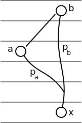
Figure 1: Path invariance during insertion of an edge $\{a,b\}$

(Refer to Figure 1) Before the insertion of $\{a,b\}$, let $p_{a}=path_{a}(a,x)$, and $p_{b}=path_{b}(b,x)$. Without loss of generality, let $|p_{a}|\leq|p_{b}|$. Now we can show that $b$ does not lie on $p_{a}$. If $b$ does lie on $p_{a}$, then $p_{a}=path_{a}(a,x)=path_{a}(a,b)\cup path_{a}(b,x)$, and $|p_{a}|=|path_{a}(a,b)|+|path_{a}(b,x)|$. Since $a$ and $b$ are distinct vertices, $|path_{a}(a,b)|>0$, and since $|path_{b}(b,x)|$ is the shortest path between the vertices $b$ and $x$, $|path_{a}(b,x)|\geq|path_{b}(b,x)|$. Hence, $|p_{a}|=|path_{a}(a,b)|+|path_{a}(b,x)|>|path_{a}(b,x)|\geq|path_{b}(b,x)|=|p_{b}|$ which is a contradiction. Hence, $b$ cannot lie on $p_{a}$.

Since $|p_{a}|\leq|p_{b}|$ and $b$ does not lie on $p_{a}$, the insertion of edge $\{a,b\}$ does not change the shortest distance between $a$ and $x$. If the shortest distance changes, then the new path will be $\{a,b\}\cup path_{b}(b,x)$, and $1+|p_{b}|<|p_{a}|$, which would be a contradiction. A similar thing happens if $|p_{b}|\leq|p_{a}|$. Hence, for every $x$, either $p_{a}$ or $p_{b}$ remains unchanged. ∎

Since the level of vertex $x$ remains invariant in atleast one BFS tree, this fact can be used to modify the level of (and subsequently even the paths to) $x$ using this invariant. This fact will be crucial in the queries that we write next.

To update the $BFSEdge$ and $Path$ relations, since we will create the new shortest path by joining together two different paths, we need to ensure that these paths are disjoint.

Without loss of generality, let $|path_{b}(b,x)|\leq|path_{a}(a,x)|$

Lemma 2.

If any vertex $t$ is on $path_{b}(b,x)$ and on $path_{v}(v,a)$, then the shortest path from $v$ to $x$ does not change after insertion of the edge $\{a,b\}$

Proof.

Consider Figure 2.

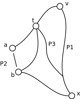
Figure 2: Disjointness of $path_{v}(v,a)$ and $path_{b}(b,x)$

Let $P_{1}=path_{v}(v,x)$. Let $P_{2}$ be the walk formed by the concatenation of $path_{v}(v,a)$, the edge $\{a,b\}$, and $path_{b}(b,x)$ (the walk is a collection of edges, possibly repeated). Let $P_{3}$ be the walk formed by the concatenation of $path_{v}(v,t)$ and $path_{b}(t,x)$. Since the walk $P_{3}$ was present even before the insertion of edge $\{a,b\}$, $|P_{3}|\geq|P_{1}|$. Since $P_{3}$ is a subset of $P_{2}$, $|P_{2}|\geq|P_{3}|$. Hence, $|P_{2}|\geq|P_{1}|$, as required. ∎

The queries during insertion of edge $\{a,b\}$ are as given and illustrated in B.1.1, and illustrated in 9. The correctness of the queries follows from Lemma 1 and Lemma 2.

4.2.2 $delete(a,b)$

Consider now the deletion of some edge $\{a,b\}$ from the graph. If it is present in the BFS tree of some vertex $v$, the removal of the edge splits the tree into two different trees. Let $R_{1}=\{u\ |\ v,u\mbox{ are connected in }V_{G}\backslash\{a,b\}\}$, and $R_{2}=\{u\ |\ u\notin R_{1}\}$. We find the set $PR=\{(p,r)\ |\ p\in R_{1}\wedge r\in R_{2}\wedge Edge(p,r)\}$, where $PR$ is the set of edges in the graph that connect the trees $R_{1}$ and $R_{2}$. The new path to $x$ will be a path from $v$ to $p$ in the BFS-tree of $v$, edge $\{p,r\}$, and path from $r$ to $x$ in the BFS-tree of $r$; and $\{p,r\}$ will be chosen to yield the shortest such path, and we will choose $\{p,r\}$ to be the lexicographically smallest amongst all such edges that yield the shortest path.

The only thing we need to address is the fact that the path from $r$ to $x$ in the BFS tree of $r$ does not pass through the edge $\{a,b\}$.

Lemma 3.

When an edge $\{a,b\}$ separates a set of vertices $R_{2}$ from the BFS tree of $v$, and $r$ and $x$ are vertices belonging to $R_{2}$, then $path_{r}(r,x)$ cannot pass through edge $\{a,b\}$

Proof.

Refer to Figure 3.

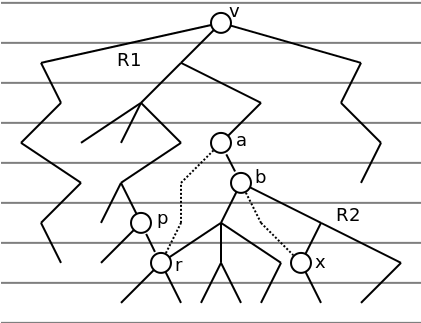
Figure 3: Deletion of edge $\{a,b\}$ and the subsequent changes (the lines represent levels in the BFS tree of vertex $v$)

We prove by contradiction. Let the shortest path from $r$ to $x$ pass through the edge $\{a,b\}$. For any two vertices $s$ and $t$, $|path_{s}(s,t)|=|path_{t}(t,s)|$, though $path_{s}(s,t)$ may not be equal to $path_{t}(t,s)$, since there can be only one value of shortest path in an undirected graph, though any number of such paths. Hence $|path_{r}(r,a)|=|path_{a}(a,r)|=1+|path_{b}(b,r)|=1+|path_{r}(r,b)|$. Also, $|path_{a}(a,x)|=1+|path_{b}(b,x)|$. If $path_{r}(r,x)$ passes through$\{a,b\}$, $|path_{r}(r,x)|=|path_{r}(r,a)|+|path_{a}(a,x)|=2+|path_{r}(r,b)|+|path_{b}(b,x)|$. But $path_{r}(r,b)\cup path_{b}(b,x)$ is a path from $r$ to $x$, and is shorter by atleast $2$ units from our claimed shortest path from $r$ to $x$. Hence, $path_{r}(r,x)$ cannot pass through $\{a,b\}$. ∎

Remark 1.

An important observation is that the above lemma holds only for the “undirected” case. It fails for the directed case, implying that the same relations cannot be used for BFS in directed graphs. To see a simple counter-example, note that there can be a directed edge from $r$ to $a$ in the directed case, and in that case, the shortest path from $r$ to $x$ can pass through $(a,b)$.

Also note that for every vertex $x$ in $R_{1}$, the shortest path from $v$ to $x$ remains the same, since removal of an edge cannot decrease the shortest distance.

The queries during deletion of edge $\{a,b\}$ are given in B.1.2. (Refer to Figure 3 for illustration on selection of edge $\{p,r\}$)

Remark 2.

Note that although we pick the new paths for every vertex in the set $R_{2}$ in parallel, we need to ensure that the paths picked are consistent, i.e. the paths form a tree and no cycle is formed. This is straightforward to see, since if a cycle is formed, it is possible to pick another path for some vertex that came earlier in the lexicographic ordering. Hence, our queries are consistent.

This leads us to the following theorem:

Theorem 3.

Breadth-First-Search for an undirected graph is in DynFO.

Note on the nature of deletion in DynFO:

One thing that is not completely clear about the complexity class DynFO is that somehow maintaining the relations in DynFO during insertion of edges (or tuples) is far easier than during deletion. A case in point is the problem of reachability in directed graphs, for which relations can be maintained that answer the problem query during insertion of edges, but whether there exist relations that can answer the query (reachability in directed graphs) during both insertion and deletion is an open problem. A particular reason for this hardness arising during deletion maybe the fact that we always begin with an empty graph. Hence, we have all the information for some point uptil an edge is inserted, which just adds some new information. But when an edge is deleted, we would need all the information about the graph that is formed from the empty graph by inserting edges upto the point that this (deleted) edge is not inserted, but that may not be possible using only polynomial space. To illustrate what we mean, consider insertion of edges in the sequence - $e_{1},e_{2},e_{3},e_{4},e_{5}$. Now if the edge $e_{3}$ is deleted, the relations do not have enough information, i.e. they do not have the tuples that would have been formed if the edges were instead inserted in the sequence $e_{1},e_{2},e_{4},e_{5}$ to an empty graph. We can try to go past this problem of monotonicity by storing all the information for all the possible sequences of insertion, but that would require storing exponential amount of data, an we would no longer remain in polynomial space, and thus not in DynFO.

Another thing that one may try is to begin with a complete graph instead of an empty graph, and then try the deletion process. This would make the deletion process extremely easy (it would act exactly as a dual of insertion), but to begin with, we would need tuples required for the entire graph. This would itself require either a lot of computation, and would beat the purpose of solving the problem in DynFO, or exponential space, in which case the problem would no longer be in DynFO.

5 3-connected Planar Graph Isomorphism

The ideas and the techniques hitherto developed implied for both the states A and B as stated in part IV of Preliminaries (2). Now onwards, our relations would no longer hold for general graphs, and we restrict ourselves to 3-connected and planar graphs, or state $A$ mentioned therein.

We shall now show how to maintain a canonical description of a 3-connected planar graph in DynFO. To achieve this end, we shall maintain Canonical Breadth-First Search (abbreviated CBFS) trees similar to the ones used by Thierauf and Wagner [15].

5.1 Canonical Breadth-First Search Trees

We shall define CBFS trees here for the sake of completeness. A theorem of Whitney [16] says that 3-connected planar graphs have a unique embedding on the sphere. Intuitively, it states a topological fact that there is one and only one way to order the edges around each vertex if a graph has to remain 3-connected and planar. This fact is used by Thierauf and Wagner to construct the CBFS trees.

Consider a 3-connected planar graph and a vertex $v$ in it. Let $N(v)=\{u:\ Edge(v,u)\}$, that is, $N(v)$ is the set of neighbours of vertex $v$. Let $D(v)=\{0,1,2,...,d_{v}-1\}$ where $d_{v}=|N(v)|$, the degree of the vertex $v$. Consider a permutation $\pi_{v}:N(v)\rightarrow D(v)$, such that for some $v_{1},v_{2}\in N(v)$, if $(v,v_{2})$ is $i$’th edge encountered while moving anti-clockwise from the edge $(v,v_{1})$, then $\pi_{v}(v_{2})=(\pi_{v}(v_{1})+i)$ mod $d_{v}$. Also, as defined in the part I of Preliminaries (2), $\pi=\{\pi_{v}\ |\ v\in V_{G}\}$, and $\pi^{c}=\{\pi_{v}^{c}\ |\ v\in V_{G}\}$.

We now define the Canonical Breath-First Search method. We need a designated vertex and an edge to begin with. Let $v$ be the vertex, and $v_{e}$ be another vertex such that $(v,v_{e})$ is the designated edge. The Canonical BFS tree thus formed will be designated as $[v,v_{e}]$. Informally, we sequentially add the edges starting from $(v,v_{e})$, and then moving from $v_{e}$ towards other vertices as per the rotation $\pi_{v}$. For every other vertex $u$, we consider the edges according to $\pi_{u}$, beginning with the edge $(u,u_{p})$, where $u_{p}$ is the parent edge of $u$ in the CBFS tree.

Formally, the pseudocode for $[v,v_{e}]$, according to some $\pi$ is as described in C.1.

Conider figure 4. If we had to perform BFS starting from vertex $u$ as per the numbering around every vertex as shown, the sequence of vertices visited around $u$ would be $x,v,w$. We would then start with $x,$ and the sequence would be $w,y,u$, but since $w$ and $u$ are already visited, we just visit $y$.

The way the numbering around every vertex is chosen given the starting edge $(u,x)$ is as follows: We first number vertices around $u$, and hence the vertices $x,v,w$ get the numbers $0,1,2$ (or $1,2,3$) around $u$. Next, for every vertex in the queue, we give its parent the number $0$, and give increasing numbers to the remaining vertices in anti-clockwise order. Hence, the numbering around $x$ would be $u,w,y$ with the numbers $0,1,2$. The resulting numbering is as shown in Figure 6.

Figure 4: Canonical Breadth-First Search Method for some anti-clockwise embedding, starting from $u$

We maintain a CBFS tree, denoted by $[v,v_{e}]$, from each vertex $v$ in the graph, for each edge $(v,v_{e})$ used as the starting embedding edge. This set of CBFS trees will help us in maintaining the necessary relations, during insertions and deletions, for isomorphism.

We need to slightly modify our previous conventions as used in the case of BFS trees, since now the CBFS trees depend not only on the vertices, but also on the chosen edge. Let $path_{v,v_{e}}(\alpha,\beta)$ denote the path from vertex $\alpha$ to $\beta$, in the CBFS tree $[v,v_{e}]$. The other notations remain same.

Let Least Common Ancestor (LCA) of $x$ and $y$, $lca_{v,v_{e}}(x,y)$, denote that vertex $d$ which is on $path_{v,v_{e}}(v,a)$ and $path_{v,v_{e}}(v,x)$ and whose level is maximum amongst all such vertices.

Denote the embedded number of vertex $x$ around vertex $u$ by $emnum_{u}(x)$, i.e. $emnum_{u}(x)=\pi_{u}(x)$. Let $parent_{v,v_{e}}(u,u_{p})$ be true if $u_{p}$ is the parent of $u$ in $[v,v_{e}]$. Denote by $emnum_{v,v_{e}}(u,x)=(\pi_{u}(x)-\pi_{u}(u_{p}))$ mod $d_{u}$, the embedded number of some vertex $x$ around $u$ in $[v,v_{e}]$ if $u_{p}$ (the parent of $u$ in $[v,v_{e}]$) has been assigned the number $0$ (or the minimum embedding number).

Since the embedding $\pi$ is unique, given a vertex and an edge incident on it, the entire CBFS tree is fixed. As such, given $v,v_{e}$, the length of the shortest path to a vertex $x$ is fixed. The actual path is decided by the following definition.

Definition 2.

Let $<_{c}$ denote a canonical ordering on paths. Let $P_{1}=path_{v,v_{e}}(v,x_{1})$ and $P_{2}=path_{v,v_{e}}(v,x_{2})$. Let $d=lca_{v,v_{e}}(x_{1},x_{2})$, $d_{1}$ a vertex on $P_{1}$ and $d_{2}$ a vertex on $P_{2}$, and $(d,d_{1})$ and $(d,d_{2})$ edges in the graph.

Then $P_{1}<_{c}P_{2}$ if:

• $|P_{1}|<|P_{2}|$ or

• $|P_{1}|=|P_{2}|$ and $emnum_{v,v_{e}}(d,d_{1})<emnum_{v,v_{e}}(d,d_{2})$
  

We shall now see how to maintain the CBFS trees $[v,v_{e}]$.

We maintain the following relations:

• $Emb(v,x,n_{x})$, meaning that the vertex $x$ is in the neighbourhood of $v$, and the edge $(v,x)$ around $v$ has the embedded number $n_{x}$;

• $Face(f,x,y,z)$, meaning that the vertex $z$ is in the anti-clockwise path from vertex $x$ to vertex $y$, around the face labelled $f$.

  Two things need to be said here. Since the number of faces in a planar graph with $n$ vertices can be more than $n$, we should label the face with a 2-tuple instead of a single symbol; but we do not do this since it adds unnecessary technicality without adding any new insight. If required, all the queries can be maintained for the faces labelled as two tuples $f=(f_{1},f_{2})$.

  Also, we maintain the transitive closure of edges around each face, instead of simply the edges that constitute each face, since the splitting and merging of faces cannot be maintained in DynFO by just maintaining the set of edges. This will become clear later in further sections that maintain the $Face$ relation;

• $Level(v,x,l)$, meaning that the vertex $x$ is at level $l$ in the BFS tree of $v$. This is exactly as in the general case.

• $CBFSEdges(v,v_{e},s,t)$, where $(s,t)$ is an edge in the CBFS tree $[v,v_{e}]$

• $CPath(v,v_{e},x,y,z)$ denoting that $z$ is on the path from $x$ to $y$ in $[v,v_{e}]$

5.2 Maintaining $Emb(v,x,n_{x})$ and $Face(f,x,y,z)$

These two relations define the embedding of the graph in the plane. Before proceeding, the following lemmas are required. Note that these lemmas will also be required for maintaining other relations as mentioned above. We further assume throughout in this section that the embedded numbering is the anti-clockwise one, and note that the same relations that we maintain for the anti-clockwise embedding can be maintained for the clockwise embedding.

Lemma 4.

In a 3-connected planar graph $G$, two distinct vertices not connected by an edge cannot both lie on two distinct faces unless $G$ is a cycle.

Proof.

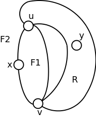
Figure 5: Two distinct vertices can lie on atmost 1 face in a 3-connected planar graph

(Refer to Figure 5) We prove by contradiction. Assume there exists such a pair of vertices $(u,v)$. We show that $(u,v)$ forms a separating pair. Consider the face $F_{1}$, the outer face $F_{2}$ and the region $R$ representing the remaining graph. Consider a vertex $x$ on a path from $u$ to $v$ and another vertex $y$ in $R$. Since the graph is 3-connected, there exist 3 distinct paths between $x$ and $y$, by Menger’s theorem. Since $x$ lies on $F_{1}$ and $F_{2}$, the path from $x$ to $y$ must pass through atleast one of these faces, by Jordan’s Curve theorem. But that will split faces $F_{1}$ or $F_{2}$ into two distinct regions. As such, any path from $x$ to $y$ must pass through $u$ or $v$, making $(u,v)$ a separating pair. The other case is when the region $R$ is empty, which makes G a cycle. ∎

As a corrollary to the above theorem, we get:

Corollary 1.

In a 3-connected planar graph $G$, two distinct vertices when connected by an edge splits one face into two new faces, creating exactly $1$ new face.

Now, due to the above theorem, we can update the $Emb$ and the $Face$ relations.

5.2.1 $insert(a,b)$

Any edge $\{a,b\}$ that is inserted lies on a particular face, say $f$. Consider the edges from vertex $a$. Since $a$ lies on the face $f$, exactly two edges from $a$ will lie on the boundary of $f$. Let these two edges, considered anti-clockwise be $e_{1}$ and $e_{2}$, having the embedded numbering $n_{1}$ and $n_{2}$, respectively. Note that $n_{2}=(n_{1}+1)$ mod $d_{a}$, where $d_{a}$ is the degree of $a$. This is because if this was not so, there would be some other edge in the anti-clockwise direction between $e_{1}$ and $e_{2}$, which would mean either we have selected a wrong face or the wrong edges $e_{1}$ and $e_{2}$.

Hence, when we insert the new edge $\{a,b\}$, we can give $\{a,b\}$ the embedded number $n_{2}$, and all the other edges around $a$ which have an embedded number more than $n_{2}$, can be incremented by $1$. Similarly we do this for $b$.

The queries in a high-level form during insertion are given in C.2.1. An illustration of the queries is given in Figure 10.

5.2.2 $delete(a,b)$

Since we are in state A as mentioned in the Preliminaries part IV, we expect the graph to be 3-connected and planar once the edge $(a,b)$ is removed. Hence by the converse of Lemma 4 above, exactly two faces will get merged. As such, our queries now will be the exact opposite to those for insertion.

The queries in a high-level form during deletion are given in C.2.2.

5.2.3 Rotating and flipping the Embedding

We will show how to rotate or flip the embedding of the graph in FOL if required, as it will be necessary for further sections.

The type of rotation that we will accomplish in this section is as follows: In any given CBFS tree $[v,v_{e}]$, for every vertex $x$, we rotate the embedding around $x$ until its parent gets the least embedding number, number $0$ (that is the $0$’th number in the ordering). For the root vertex $v$ which has no parent, we give $v_{e}$ the least embedding number.

This scheme is like a’normal’ form for ordering the edges around any vertex, or ’normalizing’ the embedding. We show in this section that this can be done in FOL. Also, flipping the ordering from anti-clockwise to clockwise is (very easily) in FOL.

We shall create the following relation: $Emb_{p}(v,v_{e},t,x,n_{x})$, which will mean that in the CBFS tree $[v,v_{e}]$, for some vertex $t$, if the parent of $t$ is $t_{p}$, and if the edge $(t,t_{p})$ (or the vertex $t_{p}$) is given the embedded number $0$, then the edge $(t,x)$ (or the vertex $x$) gets the embedded number $n_{x}$.

Note that our relation $Emb$ was independent of any particular CBFS tree, since it depended only on the structure of the 3-connected planar graph and not on any CBFS tree we chose. But $Emb_{p}$ depends on the chosen CBFS tree. Another thing to note is that we do not maintain the relation $Emb_{p}$ in our vocabulary $\tau$, since it can be easily created in FOL from the rest of the relations whenever required.

We create the relation $Emb_{p}$ in the following manner. In every CBFS tree $[v,v_{e}]$, for every vertex $t$, we find the degree ($d_{t}$) and the parent ($t_{p}$) of $t$, and the embedded number $n_{p}$ of $t_{p}$. Then for every vertex $x$ in the neighbourhood of $t$ with embedded numbering $n_{x}$, we do $n_{x}=(n_{x}-n_{p})$ mod $d_{t}$. Refer to Figure 6 for an illustration.

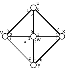
Figure 6: The CBFS tree of $[u,x]$ with the normalized rotated embedding

We also create the relation $Emb_{f}$ which will contain the flipped or the clockwise embedding $\pi^{c}$.

The queries in a high-level form for rotating and flipping the embedding are given in C.2.3.

A note said throughout in the manuscript is necessary to repeat here. Though the parent of $v$ is null in $[v,v_{e}]$, we allow the parent of $v$ to be $v_{e}$, so as to keep the queries neater. If this convention is not required, then the special case of the parent of $v$ can be handled easily by modifying the queries.

This shows that the embedding can be flipped and normalized in FOL. We conclude the following:

Theorem 4.

The embedding of a 3-connected planar graph can be maintained, normalized and flipped in DynFO.

5.3 Maintaining $CBFSEdges(v,v_{e},s,t)$ and $CPath(v,v_{e},x,y,z)$

In this section, we show how to maintain the final two relations via insertions and deletions of tuples that will help us to decide the isomorphism of two graphs. The relations are almost completely similar to the ones used for Breadth-First Search in the previous section. The only difference which arises is due to the uniqueness of the paths in Canonical Breadth-First Search Trees. We do not rewrite the $Level(v,x,l)$ since it will be exactly similar to the general BFS case.

5.3.1 $insert(a,b)$

The CBFS tree is unique if the path to every vertex $x$ from the root vertex $v$ is uniquely defined. How shall we choose the unique path? First, we consider the paths with the shortest length. This is exactly same as in Breadth-First Search seen in the previous section. But unlike BFS, where we chose the shortest path arbitrarily (that is by lexicographic ordering during insertion/deletion), we will very precisely choose one of the paths from the set of shortest paths, by Definition 2. Intuitively, Definition 2 chooses the path based on its orientation according to the embedding $\pi$.

An important observation from Definition 2 is the following: Distance has preference over Orientation. This means that if there are two paths $P_{1}$ and $P_{2}$ from $v$ to $x$ in $[v,v_{e}]$ (due to the insertion of an edge which created a cycle in the tree $[v,v_{e}]$), though $P_{2}<_{c}P_{1}$, the path $P_{1}$ will be chosen if $|P_{1}|<|P_{2}|$ irrespective of the canonical ordering $<_{c}$.

Consider some $[v,v_{e}]$. During insertion of $\{a,b\}$, let the old path (from $v$ to some $x$) be $P_{1}$ and assume that the new path $P_{2}$ passes through $(a,b)$. If $|P_{1}|<|P_{2}|$ or $|P_{1}|=|P_{2}|\wedge P_{1}<_{c}P_{2}$, the path to $x$ does not change, and all the edges and tuples to $x$ in the old relations will belong to the new relations. If $|P_{2}|<|P_{1}|$ or $|P_{1}|=|P_{2}|\wedge P_{2}<_{c}P_{1}$, the path to $x$ changes. In this case, the new path will be from $v$ to $a$ in $[v,v_{e}]$, the edge $\{a,b\}$ (from $a$ to $b$), and the path from $b$ to $x$ in $[b,b_{e}]$. The way we choose $b_{e}$ is as follows (Refer to Figure 7 for an illustration): We find the set of vertices $C$ that are adjacent to $b$ and are at $level_{v}(b)+1$. Since $a$ will be the parent of $b$ in $[v,v_{e}]^{\prime}$, we rotate the embedding around $b$ until $a$ gets the value $0$, and the choose $b_{e}$ to be the vertex in $C$ that gets the least embedding number.

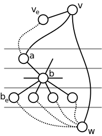
Figure 7: Choosing the vertex $b_{e}$ on the new path from $v$ to $w$

To check for the condition $P_{1}<_{c}P_{2}$, we do the following (Refer to Figure 8): We create the set $Emb_{p}$ so that the parent of each vertex has the least embedding number. Let the path $P_{a}$ denote the path from $v$ to $a$, which will be a subset of $P_{2}$. We choose the vertex which is the least common ancestor of $a$ and $x$, say $d=lca_{a,x}$, and normalize the embedding so that $d_{p}$, the parent of $d$, gets the embedding number $0$. Existence of $lca_{a,x}$ is guaranteed since $v$ lies on both $P_{1}$ and $P_{a}$. Now consider the edge $e_{1}=(lca_{a,x},d_{1})$ on $P_{1}$ and $e_{2}=(lca_{a,x},d_{2})$ on $P_{2}$. Since the embedding is normalized, we see which edge gets the smaller embedding number around the vertex $lca_{a,x}$. The path on which that edge lies will be the lesser ordered path according to $<_{c}$. It is nice to pause here for a moment and observe that this was possible since the embedding was ’normalized’, otherwise it would not have been possible.

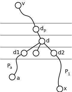
Figure 8: Illustrating $P_{a}<_{c}P_{1}$ by considering $d=lca_{a,x}$, $d_{1}$, and $d_{2}$

One more thing needs to be shown. In Lemma 1, we proved that for any vertex $x$, its level cannot change both in the BFS trees of $a$ and $b$. In the previous case of BFS, as per our algorithm, the level not being changed implied the path not being changed. But that is not the case in CBFS trees. In CBFS trees, the level not changing may still imply that the path changes (due to the $<_{c}$ ordering on paths). Hence, it may be possible that though the level of the vertex $x$ changes in only one of the CBFS trees, its actual path changes in both the CBFS trees. We need to show that this is not possible. And the reason this is necessary is because (just like the previous case) the updation of the path will depend on one specific path to vertex $x$ in the CBFS tree of $a$ or $b$ which has not changed.

Lemma 5.

After the insertion of edge $\{a,b\}$, the path to any vertex $x$, cannot change in both the CBFS trees $[a,a_{e}]$ and $[b,b_{e}]$, for all $a_{e},b_{e}$.

Proof.

Before the insertion of $\{a,b\}$, let $p_{a}=path_{a,a_{e}}(a,x)$, and $p_{b,b_{e}}=path_{b,b_{e}}(b,x)$. Without loss of generality, let $|p_{a}|\leq|p_{b}|$. It suffices to show that after the insertion of $\{a,b\}$, the path from $a$ to $x$, $p^{\prime}_{a,a_{e}}(a,x)$, is the same as $p_{a,a_{e}}(a,x)$. As seen in Lemma 1, $|p{}_{a,a_{e}}(a,x)|=|p^{\prime}_{a,a_{e}}(a,x)|\leq|p^{\prime}_{b,b_{e}}(b,x)|$. If the actual path changes, i.e. $p^{\prime}_{a,a_{e}}(a,x)\not=p_{a,a_{e}}(a,x)$, then $|p^{\prime}_{a,a_{e}}(a,x)|=1+|p^{\prime}_{a,a_{e}}(b,x)|\geq 1+|p^{\prime}_{b,b_{e}}(b,x)|\geq 1+|p_{a,a_{e}}(a,x)|>|p_{a,a_{e}}(a,x)|$ which is a contradiction. ∎

The queries in a high-level form to maintain $CBFSEdges$ and $CPath$ during insertion are given in C.3.1.

5.3.2 $delete(a,b)$

For the deletion operation, we choose the edge from $PR_{min}$ based on the $<_{c}$ relation. Note that when some edge $\{a,b\}$ is deleted, the path to some vertex $x$ in $[v,v_{e}]$ cannot change if $\{a,b\}$ does not lie on the path. Other things remain exactly similar to the general case. The queries are given in C.3.2.

6 Canonization and Isomorphism Testing

In [15], the 3-connected planar graph is canonized after performing Canonical BFS by using Depth-First Search (DFS). Performing DFS or any method that employs computing the transitive closure in any manner cannot be used here since it would not be possible in FOL, and most of the known methods of canonization seem to require computing the transitive closure. Note that a canon is required for condition 1 in Definition 1 to hold. What we seek is a method to canonize the graph, which depends only on the properties of vertices that can be inferred globally.

To achieve this, we shall label each vertex with a vector. Though the label will not be succinct now, it will be possible to create it in FOL.

Essentially, the canon for a vertex $x$ in some CBFS tree $[v,v_{e}]$ will be a set of tuples $(l,h)$ of the levels and (normalized) embedding numbers of ancestors of $x$.

Definition 3.

Let canon for each vertex $x$ in $[v,v_{e}]$ be represented by $Canon_{v,v_{e}}(x)$. Then,

$${\displaystyle Canon_{v,v_{e}}(x)=\{(l,h):\;\exists q,q_{p},\ C\ \wedge\ L\ \wedge\ P\ \wedge\ H\}}$$

where,

• ${\displaystyle C:\ CPath(v,v_{e},v,x,q),}$

• ${\displaystyle L:\ l=level_{v}(q)}$,

• ${\displaystyle P:\ parent_{v,v_{e}}(q,q_{p})}$,

• ${\displaystyle H:\ h=emnum_{v,v_{e}}(q_{p},q)}$
  

Lemma 6.

For any CBFS tree $[v,v_{e}]$, for any two vertices $x$ and $y$, $x=y\Leftrightarrow Canon(x)=Canon(y)$

Proof.

If two vertices are same, they have the same canon. If they are different, it suffices to show that the canons necessarily differ at one point. Let $d=lca_{v,v_{e}}(x,y)$. Since $d$ is the least common ancestor, the path to $x$ and $y$ splits at $d$. From Definition 2, $(d,d_{x})$ and $(d,d_{y})$ are distinct edges, and they have a different embedding number. Hence the canons for $x$ and $y$ are necessarily different at the level of $d_{x}$ and $d_{y}$. ∎

It is now easy to canonize each of the CBFS trees in FOL. Once each vertex has a canon, each edge is also uniquely numbered. The main idea is this: A canon will in itself encode all the necessary properties of the vertex, and the set of canons of all vertices become the signature of the graph, preserving edges. The main advantage of Definition 3 is that the canon of the graph can be generated in FOL. It’s worthwhile to observe how this neatly beats the otherwise inevitable computation of transitive closure (Theorem 1) to canonize the graph.

Hence, two 3-connected planar graphs $G$ and $H$ are isomorphic if and only if for some CBFS tree $[g,g_{e}]$ of $G$, there is a CBFS tree $[h,h_{e}]$, such that:

• $\forall x\exists y,\;(x\in G\wedge y\in H\wedge(Canon(x)=Canon(y)))$ and

• $\forall x_{1},x_{2},\;((Edge(x_{1},x_{2})\in G)\Leftrightarrow(Edge(Canon(x_{1}),Canon(x_{2}))\in H))$

$H$ implies either $H$ with the embedding $\rho$ or $H$ with flipped embedding $\rho^{-1}$. It is evident that if the graphs are isomorphic, there will be some CBFS tree in $G$ and $H$ whose canons will be equivalent in the above sense. If the graphs are not isomorphic, no canon of any CBFS tree could be equivalent, since it would then directly give a bijection between the vertices of the graph that preserves the edges, which would be a contradiction.

Since we still need to precompute all the relations before the condition of 3-connectivity is reached, isomorphism of $G$ and $H$ is in $\textsf{{{{DynFO}}}}^{+}$. This brings us to the main conclusion of this section:

Theorem 5.

3-connected planar graph isomorphism is in $\textsf{{{{DynFO}}}}^{+}$

7 Conclusions

We have proven that Breadth-First Search for undirected graphs can be performed in DynFO and isomorphism for Planar 3-connected graphs can be decided in $\textsf{{{{DynFO}}}}^{+}$. A natural extension is to show that Planar Graph Isomorphism is in DynFO. Though even parallel algorithms for this problem are known [4], the ideas cannot be directly employed because of myriad problems arising due to automorphisms of the bi/tri-connected component trees (which are used in [4]), and various subroutines that require computing the transitive closure. In spite of these shortcomings, we strongly believe that Planar Graph Isomorphism is in DynFO, though the exact nature of the queries still remains open.

8 Acknowledgements

The author sincerely thanks Samir Datta for fruitful discussions and critical comments on all topics ranging from the problem statement to the preparation of the final manuscript.

Appendix A Arithmetic

A.1 Relations: Sum

A.1.1 $insert(a,b)$

Updating the relation $Sum$ during insertion:

• A tuple $(t,x,y)$ belongs to $Sum^{\prime}$ if:
  
  {case in which there is no element in the universe}
  $t=x=y=a\ \wedge\ \neg U(a)\wedge\forall u(O^{\prime}(a,u)$
  OR
  
  {adding the relation $a+0=a$}
  $min\leftarrow min:\ \forall u,\,U(u)\Rightarrow O(min,u)$
  $t=a\wedge((x=a\wedge y=min)\vee(x=min\wedge y=a))$
  OR
  
  $max\leftarrow max:$$\forall u,\,U(u)\Rightarrow O(u,max)$
  {$max$ is the maximum element. Note that if $a$ is a new element inserted in the universe, $max+1=a$}
  $Sum(t,x,y)\vee(t=a\wedge(Sum(max,x-1,y)\vee Sum(max,x,y-1)))$
  

(Back to Section 3.3)

Appendix B Breadth-First Search

B.1 Relations: Level, BFSEdge, BFSPath

B.1.1 $insert(a,b)$

The relations $Level$, $BFSEdge$, and $BFSPath$ are updated during insertion a follows: {The queries are illustrated in Figure 9}

• A tuple $(v,x,l)$ belongs to $Level^{\prime}$, if:
  ${\displaystyle l_{old}\leftarrow level_{v}(x)}$ {$l_{old}\leftarrow\infty$ if there is no $l_{old}$ such that $Level(v,x,l_{old})$ holds}
  IF $level_{a}(x)\leq level_{b}(x)$: $\alpha\leftarrow b,$ $\beta\leftarrow a$; ELSE: $\alpha\leftarrow a,$ $\beta\leftarrow b$
  $l_{new}\leftarrow level_{v}(\alpha)+1+level_{\beta}(x)$
  $l=\min(l_{old},l_{new})$
  

• A tuple $(v,x,y)$ belongs to $BFSEdge^{\prime}$, if:
  $\exists w$ such that
  $l_{old}\leftarrow level_{v}(w)$, $l_{new}\leftarrow level^{\prime}_{v}(w)$,
  IF $level_{a}(w)\leq level_{b}(w)$: $\alpha\leftarrow b,$ $\beta\leftarrow a$; ELSE: $\alpha\leftarrow a,$ $\beta\leftarrow b$
  
  {the level of $w$ did not change and $\{x,y\}$ was on a path from $v$ to $w$}
  $l_{new}=l_{old}$ and $Path(v,v,w,\{x,y\})\wedge BFSEdge(v,x,y)$
  OR
  
  {the level of $w$ changed and $\{x,y\}$ lies on the new path}
  $l_{new}<l_{old}$ and
  $(Path(v,v,\alpha,\{x,y\})\wedge BFSEdge(v,x,y))$ {Path from $v$ to $\alpha$}
  $\vee(Path(\beta,\beta,w,\{x,y\})\wedge BFSEdge(\beta,x,y))$ {Path from $\beta$ to $w$}
  $\vee(x=a\wedge y=b)$$\vee(x=b\wedge y=a)$ {$\{x,y\}$ is the edge $\{a,b\}$}
  

• A tuple $(v,x,y,z)$ belongs to $Path^{\prime}$, if:
  $\exists w$ such that
  $l_{old}\leftarrow level_{v}(w)$, $l_{new}\leftarrow level^{\prime}_{v}(w)$,
  IF $level_{a}(w)\leq level_{b}(w)$: $\alpha\leftarrow b,$ $\beta\leftarrow a$; ELSE: $\alpha\leftarrow a,$ $\beta\leftarrow b$
  
  {the level of $w$ did not change and $\{x,y\}$ was on a path from $v$ to $w$}
  $l_{new}=l_{old}$ and $Path(v,v,w,\{x,y,z\})\wedge Path(v,x,y,z)$
  OR
  
  {the level of $w$ changed, and the vertices $x,y,z$ lie on the new path}
  $l_{new}<l_{old}$ and
  $(Path(v,v,\alpha,\{x,y,z\})\wedge Path(v,x,y,z))$ {All on the path from $v$ to $\alpha$}
  $\vee(Path(\beta,\beta,w,\{x,y,z\})\wedge Path(\beta,x,y,z))$ {All on the path from $\beta$ to $w$}
  $\vee(Path(v,v,\alpha,\{x\})\wedge Path(\beta,\beta,w,\{y,z\})\wedge Path(\beta,\beta,y,z))$ {$x$ on $path_{v}(v,\alpha)$ and $y,z$ on $path_{\beta}(\beta,w)$}
  $\vee(Path(v,v,\alpha,\{x,z\})\wedge Path(v,v,z,x)\wedge Path(\beta,\beta,w,y))$ {$x,z$ on $path_{v}(v,\alpha)$ and $y$ on $path_{\beta}(\beta,w)$}
  
  

  

  Figure 9: $BFSEdge$ and $Path$ during insertion of edge $\{a,b\}$

(Back to Section 4.2.1)

B.1.2 $delete(a,b)$

The relations $Level$, $BFSEdge$, and $BFSPath$ are updated during deletion are as follows (Refer to Figure 3 for illustration of relations used):

• $R_{2}(v,x)=BFSEdge(v,a,b)\wedge Path(v,v,x,\{a,b\})$
  $R_{1}(v,y)=\neg R_{2}(v,y)$
  $PR(v,s,t)=R_{1}(v,s)\wedge R_{2}(v,t)\wedge Edge(s,t)$ {All edges connecting $R_{1}$ and $R_{2}$}
  $l_{min}(v,w)\leftarrow\min\{level_{v}(s)+1+level_{t}(w):\;PR(v,s,t)\}$ {Length of the new shortest path from $v$ to $w$}
  $PR_{min}(v,w,s,t)=R_{2}(v,w)\wedge PR(v,s,t)\wedge(level_{v}(s)+1+level_{t}(w)=l_{min}(v,w))$ {Set of edges that lead to the shortest path}
  $PR_{lex,min}(v,w,s,t)=PR_{min}(v,w,s,t)\wedge(s\leq t)\wedge(\forall p,q,\;PR_{min}(v,w,p,q)\Rightarrow(s<p)\vee((s=p)\wedge(t\leq q)))$
  {Choosing the lexicographically smallest edge. $PR_{lex,min}$ is the set of new edges that will be added. The queries are now exactly similar to insertion of edges}

• A tuple $(v,x,l)$ belongs to $Level^{\prime}$ if:
  
  {$\{a,b\}$ did not belong to $v$’s BFS tree}
  $\neg BFSEdge(v,a,b)\wedge Level(v,x,l)$
  OR
  $BFSEdge(v,a,b)\wedge l=l_{min}(v,x)$
  

• A tuple $(v,x,y)$ belongs to $BFSEdge^{\prime}$ if:
  $\exists w$ such that
  
  {$\{a,b\}$ was not and $\{x,y\}$ was on the path from $v$ to $w$}
  $\neg Path(v,v,w,\{a,b\})\wedge Path(v,v,w,\{x,y\})\wedge BFSEdge(v,x,y)$
  OR
  
  {$\{x,y\}$ lies on the new path from $v$ to $w$}
  $p,r\leftarrow PR_{lex,min}(v,w,p,r)$
  $(Path(v,v,w,\{a,b\})\wedge Path(v,v,p,\{x,y\})\wedge BFSEdge(v,x,y))$ {edge $\{x,y\}$ is on $path_{v}(v,p)$}
  $\vee(Path(r,r,w,\{x,y\})\wedge BFSEdge(r,x,y))$ {edge $\{x,y\}$ is on $path_{r}(r,w)$}
  $\vee((x=p)\wedge(y=r))\vee((x=r)\wedge(y=p))$ {$\{x,y\}$ is the edge $\{p,r\}$}
  

• A tuple $(v,x,y,z)$ belongs to $Path^{\prime}$ if:
  $\exists w$ such that
  
  {path from $v$ to $w$ is unchanged, and $z$ is on path from $x$ to $y$ in BFS tree of $v$}
  $\neg Path(v,v,w,\{a,b\})\wedge Path(v,v,w,\{x,y,z\})\wedge Path(v,x,y,z)$
  OR
  
  {$\{x,y,z\}$ lies on the new path from $v$ to $w$}
  $p,r\leftarrow PR_{lex,min}(v,w,p,r)$
  $(Path(v,v,w,\{a,b\})\wedge Path(v,v,p,\{x,y,z\})\wedge Path(v,x,y,z))$ {All of $x,y,z$ on the path from $v$ to $p$}
  $\vee(Path(r,r,w,\{x,y,z\})\wedge Path(r,x,y,z))$ {All of $x,y,z$ on the path from $r$ to $w$}
  $\vee(Path(v,v,p,\{x\})\wedge Path(r,r,w,\{y,z\})\wedge Path(r,r,y,z))$ {$x$ on $path_{v}(v,p)$ and $y,z$ on $path_{r}(r,w)$}
  $\vee(Path(v,v,p,\{x,z\})\wedge Path(v,v,z,x)\wedge Path(r,r,w,y))$ {$x,z$ on $path_{v}(v,p)$ and $y$ on $path_{r}(r,w)$}
  

(Back to Section 4.2.2)

Appendix C Canonical Breadth-First Search

C.1 Canonical Breadth-First Search Method

$Queue\leftarrow null$;

$Enqueue(v)$;

Add $(v,v_{e})$ to the CBFS tree;

WHILE $!Queue.empty()$

$u\leftarrow Dequeue()$;

$u_{p}\leftarrow u.parent()$;

{where $v.parent()$ is let to be $v_{e}$ for ease of code, though $v$’s parent is actually $null$}

$k\leftarrow\pi_{u}(u_{p})$;

$k\leftarrow(k+1)$ mod $d_{u}$;

$u^{\prime}\leftarrow\pi_{u}^{-1}(k)$;

WHILE $u^{\prime}\not=u_{p}$

IF $u^{\prime}$ is not visited

Add $(u,u^{\prime})$ to the CBFS tree;

Mark $u^{\prime}$ as visited;

$Enqueue(u^{\prime})$;

$k\leftarrow(k+1)$ mod $d_{u}$;

$u^{\prime}\leftarrow\pi_{u}^{-1}(k)$;

Algorithm 1 Canonical Breadth-First-Search Method for $(v,v_{e})$

(Back to Section 5.1)

C.2 Relations: Emb, Face

C.2.1 $insert(a,b)$

Updating the relations $Emb$ and $Face$ during insertion. {Refer to Figure 10 for an illustration and intuition for the following queries}

• $f_{ab}\leftarrow Face(f_{ab},a,b,b)$ {Face on which both $a$ and $b$ lie}
  $a_{2}\leftarrow Edge(a,a_{2})\wedge(\forall z,Face(f_{ab},a_{2},a,z)\Rightarrow z=a\vee z=a_{2})$
  $b_{2}\leftarrow Edge(b,b_{2})\wedge(\forall z,Face(f_{ab},b_{2},b,z)\Rightarrow z=b\vee z=b_{2})$
  $n_{a_{2}}\leftarrow Emb(a,a_{2},n_{a_{2}})$
  $n_{b_{2}}\leftarrow Emb(b,b_{2},n_{b_{2}})$
  

• A tuple $(v,x,n_{x})$ belongs to $Emb^{\prime}$ if:
  
  {$v$ is not affected by the insertion of $\{a,b\}$}
  $(v\not=a)\wedge(v\not=b)\wedge Emb(v,x,n_{x})$
  OR
  
  {the tuple has the new embedding number given by $a$ to $b$ or $b$ to $a$}
  $(v,x,n_{x})=(a,b,n_{a_{2}})\vee(b,a,n_{b_{2}})$
  OR
  
  {the tuple represents a vertex around $a$ or $b$ whose embedding number has not changed}
  $((v=a)\wedge Emb(v,x,n_{x})\wedge(n_{x}<n_{a_{2}}))$
  $\vee((v=b)\wedge Emb(v,x,n_{x})\wedge(n_{x}<n_{b_{2}}))$
  OR
  
  {the tuple represents a vertex around $a$ or $b$ whose embedding number has increased by 1}
  $((v=a)\wedge Emb(v,x,n_{x}-1)\wedge(n_{x}\geq n_{a_{2}}))$
  $\vee((v=b)\wedge Emb(v,x,n_{x}-1)\wedge(n_{x}\geq n_{b_{2}}))$
  

• A tuple $(f,x,y,z)$ belongs to $Face^{\prime}$ if:
  
  {the face was not the one on which both $a$ and $b$ were there}
  $f\not=f_{ab}\wedge Face(f,x,y,z)$
  OR
  
  {the face is split into 2 faces}
  $S_{1}(z)=Face(f_{ab},a,b,z)$ {Splitting all vertices into 2 sets, for each new face}
  $S_{2}(z)=Face(f_{ab},b,a,z)$
  $f_{p}\leftarrow f_{ab}$ {Name for the first face}
  $F(u)=$$\forall x,y,z,\neg Face(u,x,y,z)$
  $f_{q}\leftarrow F(f_{q})\wedge\forall x,F_{q}(x)\Rightarrow f_{q}\leq x$ {choosing the lexicographically smallest available label}
  $(f=f_{p}\wedge S_{1}(\{x,y,z\}))\vee(f=f_{q}\wedge S_{2}(\{x,y,z\}))$
  

  

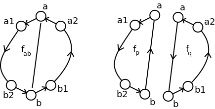
  Figure 10: Splitting (during insertion) and Merging (during deletion) of face(s)

(Back to Section 5.2.1)

C.2.2 $delete(a,b)$

Updating the relations $Emb$ and $Face$ during deletion. {Refer to Figure 10 for an illustration and intuition for the following queries}

• $f_{p}=Face(f_{p},a,b,b)\wedge(\forall x,Face(f_{p},b,a,x)\Rightarrow x=a\vee x=b)$
  $f_{q}=Face(f_{q},a,b,b)\wedge(\forall x,Face(f_{q},a,b,x)\Rightarrow x=a\vee x=b)$ {Finding the two faces on which the edge $\{a,b\}$ lies}
  $f_{ab}=\min(f_{p},f_{q})$ {Name for the new combined face}
  $n_{a}\leftarrow Emb(b,a,n_{a})$
  $n_{b}\leftarrow Emb(a,b,n_{b})$
  

• A tuple $(v,x,n_{x})$ belongs to $Emb^{\prime}$ if:
  
  {$v$ is not affected by the deletion of $\{a,b\}$}
  $(v\not=a)\wedge(v\not=b)\wedge Emb(v,x,n_{x})$
  OR
  
  {the tuple represents a vertex around $a$ or $b$ whose embedding number has not changed}
  $((v=a)\wedge Emb(v,x,n_{x})\wedge(n_{x}<n_{b}))$
  $\vee((v=b)\wedge Emb(v,x,n_{x})\wedge(n_{x}<n_{a}))$
  OR
  
  {the tuple represents a vertex around $a$ or $b$ whose embedding number has decreased by 1}
  $((v=a)\wedge Emb(v,x,n_{x}+1)\wedge(n_{x}>n_{b}))$
  $\vee((v=b)\wedge Emb(v,x,n_{x}+1)\wedge(n_{x}>n_{a}))$
  

• A tuple $(f,x,y,z)$ belongs to $Face^{\prime}$ if:
  
  {every tuple in the old relation}
  $(f\not=f_{p}\wedge f\not=f_{q}\wedge Face(f,x,y,z))$
  $\vee(f=f_{ab}\wedge(Face(f_{p},x,y,z)\vee Face(f_{q},x,y,z)))$ {transferring all tuples of $f_{p}$ and $f_{q}$ to $f_{ab}$}
  OR
  
  {the tuple forms paths between vertices from one face to those in the other}
  $(f=f_{ab}\wedge Face(f_{p},a,x,x)\wedge Face(f_{q},b,y,z))$ {$x$ in $f_{p}$, $y,z$ in $f_{q}$}
  $\vee(f=f_{ab}\wedge Face(f_{q},b,x,x)\wedge Face(f_{p},a,y,z))$ {$x$ in $f_{q}$, $y,z$ in $f_{p}$}
  $\vee(f=f_{ab}\wedge Face(f_{p},a,z,x)\wedge Face(f_{q},b,y,y))$ {$x,z$ in $f_{p}$, $y$ in $f_{q}$}
  $\vee(f=f_{ab}\wedge Face(f_{q},b,z,x)\wedge Face(f_{p},a,y,y))$ {$x,z$ in $f_{q}$, $y$ in $f_{p}$}
  $\vee(f=f_{ab}\wedge Face(f_{p},a,z,x)\wedge Face(f_{q},b,y,y))$ {$x,z$ in $f_{p}$, $y$ in $f_{q}$}
  $\vee(f=f_{ab}\wedge Face(f_{p},a,x,x)\wedge Face(f_{q},b,z,z)\wedge Face(f_{p},x,y,b))$ {$x$ in $f_{p}$, $z$ in $f_{q}$, $y$ in $f_{p}$}
  $\vee(f=f_{ab}\wedge Face(f_{q},b,x,x)\wedge Face(f_{p},a,z,z)\wedge Face(f_{q},x,y,a))$ {$x$ in $f_{q}$, $z$ in $f_{p}$, $y$ in $f_{q}$}
  

(Back to Section 5.2.2)

C.2.3 Rotating and Flipping the Embedding

Queries to rotate and flip the embedding in FOL.

• {$Deg(v,d_{v})$ holds if the degree of vertex $v$ is $d_{v}$}
  $Deg(v,d_{v})=(\forall u,Edge(v,u)\Rightarrow\exists n_{u},Emb(v,u,n_{u})\wedge(n_{u}<d_{v}))\wedge\exists u,n_{u},Edge(v,u)\wedge Emb(v,u,n_{u})\wedge(n_{u}+1=d_{v})$
  

• {$Parent(v,v_{e},x_{p},x)$ denotes that in $[v,v_{e}]$, vertex $x_{p}$ is the parent of vertex $x$ }
  $Parent(v,v_{e},x_{p},x)=\exists l_{p},l,Level(v,x_{p},l_{p})\wedge Level(v,x,l)\wedge(l_{p}+1=l)\wedge CBFSEdges(v,v_{e},x_{p},x)$
  

• {$EmbPar(v,v_{e},x,n_{p})$ denotes that the embedding number of $x$’s parent in $[v,v_{e}]$ is $n_{p}$}
  $EmbPar(v,v_{e},x,n_{p})=\exists x_{p},Parent(v,v_{e},x_{p},x)\wedge Emb(x,x_{p},n_{p})$
  $Emb_{p}(v,v_{e},t,x,n{}_{x})=Edge(x,t)\wedge\exists n_{p},d_{t},n_{old},Deg(t,d_{t})\wedge EmbPar(v,v_{e},t,n_{p})\wedge Emb(t,x,n_{old})$
  $\wedge(n_{old}\geq n_{p}\Rightarrow n{}_{x}=n_{old}-n_{p})\wedge(n_{old}<n_{p}\Rightarrow n{}_{x}=n_{old}+d_{x}-n_{p})$
  $Emb_{f}(v,x,n{}_{x})=\exists n_{old},d_{v},Emb(v,x,n_{old})\wedge Deg(v,d_{v})\wedge(n{}_{x}=d_{v}-1-n_{old})$
  
  (Back to Section 5.2.3)

C.3 Relations: CBFSEdges, CBFSPath

C.3.1 $insert(a,b)$

Updating the relations $CBFSEdges$ and $CBFSPath$ during insertion.

• $l_{old}\leftarrow level_{v}(w)$, $l_{new}\leftarrow level{}_{v}(a)+1+level_{b}(w)$, IF $level_{a}(w)\leq level_{b}(w)$: $\alpha\leftarrow b,$ $\beta\leftarrow a$; ELSE: $\alpha\leftarrow a,$ $\beta\leftarrow b$
  $d\leftarrow lca_{v,v_{e}}(w,a)$
  $d_{1}\leftarrow CPath(v,v_{e},d,w,d_{1})\wedge CBFSEdges(v,v_{e},d,d_{1})$
  $d_{2}\leftarrow CPath(v,v_{e},d,a,d_{2})\wedge CBFSEdges(v,v_{e},d,d_{2})$
  $n_{1}\leftarrow emnum^{\prime}_{v,v_{e}}(d,d_{1})$
  $n_{2}\leftarrow emnum^{\prime}_{v,v_{e}}(d,d_{2})$
  $C(z)=(level^{\prime}_{v}(z)=level^{\prime}_{v}(\beta)+1)\wedge Edge(\beta,z)$
  $\beta_{e}\leftarrow\min\{emnum^{\prime}_{v,v_{e}}(\beta,z):C(z)\}$
  

• A tuple $(v,v_{e},x,y)$ belongs to $CBFSEdges^{\prime}$, if
  $\exists w$ such that
  
  {$|P_{1}|<|P_{2}|$ or $|P_{1}|=|P_{2}|\wedge P_{1}<_{c}P_{2}$, and $\{x,y\}$ was on $|P_{1}|$}
  $(l_{old}<l_{new})\vee(l_{old}=l_{new}\wedge n_{1}<n_{2})$ and $CPath(v,v_{e},v,w,\{x,y\})\wedge CBFSEdges(v,v_{e},x,y)$
  OR
  
  {$|P_{2}|<|P_{1}|$ or $|P_{1}|=|P_{2}|\wedge P_{2}<_{c}P_{1}$, and $\{x,y\}$ is on $|P_{2}|$}
  $(l_{old}>l_{new})\vee(l_{old}=l_{new}\wedge n_{1}>n_{2})$ and
  $(CPath(v,v_{e},v,\alpha,\{x,y\})\wedge CBFSEdges(v,v_{e},x,y))$ {Path from $v$ to $\alpha$}
  $\vee(CPath(\beta,\beta_{e},\beta,w,\{x,y\})\wedge CBFSEdges(\beta,\beta_{e},x,y))$ {Path from $\beta$ to $w$}
  $\vee(x=a\wedge y=b)$$\vee(x=b\wedge y=a)$ {$\{x,y\}$ is the edge $\{a,b\}$}
  

• A tuple $(v,x,y,z)$ belongs to $CPath^{\prime}$, if
  $\exists w$ such that
  
  {$|P_{1}|<|P_{2}|$ or $|P_{1}|=|P_{2}|\wedge P_{1}<_{c}P_{2}$, and $\{x,y,z\}$ were on $|P_{1}|$}
  $(l_{old}<l_{new})\vee(l_{old}=l_{new}\wedge n_{1}<n_{2})$ and $CPath(v,v_{e},v,w,\{x,y,z\})\wedge CBFSEdges(v,v_{e},x,y,z)$
  OR
  
  {$|P_{2}|<|P_{1}|$ or $|P_{1}|=|P_{2}|\wedge P_{2}<_{c}P_{1}$, and $\{x,y,z\}$ are on $|P_{2}|$}
  $(l_{old}>l_{new})\vee(l_{old}=l_{new}\wedge n_{1}>n_{2})$ and
  $(CPath(v,v_{e},v,\alpha,\{x,y,z\})\wedge CPath(v,v_{e},x,y,z))$ {All on the path from $v$ to $\alpha$}
  $\vee(CPath(\beta,\beta_{e},w,\{x,y,z\})\wedge CPath(\beta,\beta_{e},x,y,z))$ {All on the path from $\beta$ to $w$}
  $\vee(CPath(v,v_{e},v,\alpha,\{x\})\wedge CPath(\beta,\beta_{e},\beta,w,\{y,z\})\wedge CPath(\beta,\beta_{e},\beta,y,z))$ {$x$ on $path_{v,v_{e}}(v,\alpha)$ and $y,z$ on $path_{\beta,\beta_{e}}(\beta,w)$}
  $\vee(CPath(v,v_{e},v,\alpha,\{x,z\})\wedge CPath(v,v_{e},v,z,x)\wedge CPath(\beta,\beta_{e},\beta,w,y))$ {$x,z$ on $path_{v,v_{e}}(v,\alpha)$ and $y$ on $path_{\beta,\beta_{e}}(\beta,w)$}
  

(Back to Section 5.3.1)

C.3.2 $delete(a,b)$

• $R_{2}(v,v_{e},x)=CBFSEdges(v,v_{e},a,b)\wedge CPath(v,v_{e}v,x,\{a,b\})$
  $R_{1}(v,v_{e},y)=\neg R_{2}(v,v_{e},y)$
  $PR(v,v_{e}s,t)=R_{1}(v,v_{e},s)\wedge R_{2}(v,v_{e},t)\wedge Edge(s,t)$ {All edges connecting $R_{1}$ and $R_{2}$}
  $l_{min}(v,w)\leftarrow\min\{level_{v}(s)+1+level_{t}(w):\;\bigcup_{v_{e}}PR(v,v_{e},s,t)\}$ {Length of the new shortest path from $v$ to $w$}
  $PR_{min}(v,v_{e},w,s,t)=R_{2}(v,v_{e},w)\wedge PR(v,v_{e},s,t)\wedge(level_{v}(s)+1+level_{t}(w)=l_{min}(v,w))$ {Set of edges that lead to the shortest path}
  $PR_{<,min}(v,v_{e},w,s,t)=PR_{min}(v,v_{e},w,s,t)\wedge$
  $(\forall p,q,\;PR_{min}(v,w,p,q)\Rightarrow(path_{v,v_{e}}(v,s)<_{c}path_{v,v_{e}}(v,p))\vee(s=p\wedge emnum_{v,v_{e}}(s,t)\leq emnum_{v,v_{e}}(s,q)))$
  {$PR_{<,min}$ is the set of new edges that will be added. The queries are now similar to insertion of edges}
  

• A tuple $(v,v_{e},x,y)$ belongs to $CBFSEdges^{\prime}$, if
  $\exists w$ such that
  
  {$\{a,b\}$ was not on $path_{v,v_{e}}(v,w)$, and $\{x,y\}$ was on $path_{v,v_{e}}(v,w)$}
  $\neg CPath(v,v_{e},v,w,\{a,b\})\wedge CPath(v,v,w,\{s,t\})\wedge CBFSEdges(v,s,t)$
  OR
  
  {$\{x,y\}$ lies on the new path from $v$ to $w$}
  $s,t\leftarrow PR_{<,min}(v,v_{e},w,s,t)$
  $C(z)=(level^{\prime}_{v}(z)=level^{\prime}_{v}(t)+1)\wedge Edge(t,z)$
  $t_{e}\leftarrow\min\{emnum^{\prime}_{v,v_{e}}(t,z):C(z)\}$
  $(CPath(v,v_{e},v,w,\{a,b\})\wedge CPath(v,v_{e},v,s,\{x,y\})\wedge CBFSEdges(v,v_{e},x,y))$ {edge $\{x,y\}$ is on $path_{v,v_{e}}(v,s)$}
  $\vee(CPath(t,t_{e},t,w,\{s,t\})\wedge CBFSEdges(t,t_{e},x,y))$ {edge $\{x,y\}$ is on $path_{t,t_{e}}(t,w)$}
  $\vee((x=s)\wedge(y=t))\vee((x=t)\wedge(y=s))$ {$\{x,y\}$ is the edge $\{s,t\}$}
  

• A tuple $(v,v_{e},x,y,z)$ belongs to $CPath^{\prime}$, if
  $\exists w$ such that
  
  {path from $v$ to $w$ is unchanged, and $z$ is on path from $x$ to $y$ in $[v,v_{e}]$}
  $\neg CPath(v,v_{e},v,w,\{a,b\})\wedge CPath(v,v_{e},v,w,\{x,y,z\})\wedge CPath(v,v_{e},x,y,z)$
  OR
  
  {$\{x,y,z\}$ lies on the new path from $v$ to $w$}
  $s,t\leftarrow PR_{<,min}(v,w,s,t)$
  $C(z)=(level^{\prime}_{v}(z)=level^{\prime}_{v}(t)+1)\wedge Edge(t,z)$
  $t_{e}\leftarrow\min\{emnum^{\prime}_{v,v_{e}}(t,z):C(z)\}$
  $(CPath(v,v_{e},v,w,\{a,b\})\wedge CPath(v,v_{e},v,s,\{x,y,z\})\wedge CPath(v,v_{e},x,y,z))$ {All of $x,y,z$ on $path_{v,v_{e}}(v,s)$}
  $\vee(CPath(t,t_{e},t,w,\{x,y,z\})\wedge CPath(t,t_{e},x,y,z))$ {All of $x,y,z$ on $path_{t,t_{e}}(t,w)$}
  $\vee(CPath(v,v_{e},v,s,\{x\})\wedge CPath(t,t_{e},t,w,\{y,z\})\wedge CPath(t,t_{e},t,y,z))$ {$x$ on $path_{v,v_{e}}(v,s)$ and $y,z$ on $path_{t,t_{e}}(t,w)$}
  $\vee(CPath(v,v_{e},v,s,\{x,z\})\wedge CPath(v,v_{e},v,z,x)\wedge CPath(t,t_{e},t,w,y))$ {$x,z$ on $path_{v,v_{e}}(v,s)$ and $y$ on $path_{t,t_{e}}(t,w)$}
  

(Back to Section 5.3.2)

References

- [1] Vikraman Arvind and Piyush P Kurur. Graph isomorphism is in spp. In Foundations of Computer Science, 2002. Proceedings. The 43rd Annual IEEE Symposium on, pages 743–750. IEEE, 2002.
- [2] Thomas H. Cormen, Clifford Stein, Ronald L. Rivest, and Charles E. Leiserson. Introduction to Algorithms. McGraw-Hill Higher Education, 2nd edition, 2001.
- [3] Samir Datta, Nutan Limaye, and Prajakta Nimbhorkar. 3-connected planar graph isomorphism is in log-space. arXiv preprint arXiv:0806.1041, 2008.
- [4] Samir Datta, Nutan Limaye, Prajakta Nimbhorkar, Thomas Thierauf, and Fabian Wagner. Planar graph isomorphism is in log-space. In Computational Complexity, 2009. CCC’09. 24th Annual IEEE Conference on, pages 203–214. IEEE, 2009.
- [5] Reinhard Diestel. Graph theory. 2005, 2005.
- [6] GZ Dong and JW Su. Incremental and decremental evaluation of transitive closure by first-order queries. Information and Computation, 120(1):101–106, 1995.
- [7] Kousha Etessami. Dynamic tree isomorphism via first-order updates to a relational database. In Proceedings of the seventeenth ACM SIGACT-SIGMOD-SIGART symposium on Principles of database systems, pages 235–243. ACM, 1998.
- [8] William Hesse. The dynamic complexity of transitive closure is in dyntc0. In In Proceedings of the 8th International Conference on Database Theory (2001. Citeseer, 2002.
- [9] WILLIAM M HESSE. Dynamic computational complexity. Computer Science, 2003.
- [10] John E Hopcroft and Jin-Kue Wong. Linear time algorithm for isomorphism of planar graphs (preliminary report). In Proceedings of the sixth annual ACM symposium on Theory of computing, pages 172–184. ACM, 1974.
- [11] Neil Immerman. Descriptive complexity. Springer, 1999.
- [12] Steven Lindell. A logspace algorithm for tree canonization. In Proceedings of the twenty-fourth annual ACM symposium on Theory of computing, pages 400–404. ACM, 1992.
- [13] Sushant Patnaik and Neil Immerman. Dyn-fo (preliminary version): a parallel, dynamic complexity class. In Proceedings of the thirteenth ACM SIGACT-SIGMOD-SIGART symposium on Principles of database systems, pages 210–221. ACM, 1994.
- [14] Thomas Schwentick. Perspectives of dynamic complexity. In Logic, Language, Information, and Computation, pages 33–33. Springer, 2013.
- [15] Thomas Thierauf and Fabian Wagner. The isomorphism problem for planar 3-connected graphs is in unambiguous logspace. Theory of Computing Systems, 47(3):655–673, 2010.
- [16] H. Whitney. A set of topological invariants for graphs. American Journal of Mathematics, 55(1):231–235, 1933.