Uncertainty Measures and Limiting Distributions for Filament Estimation
Abstract
A filament is a high density, connected region in a point cloud. There are several methods for estimating filaments but these methods do not provide any measure of uncertainty. We give a definition for the uncertainty of estimated filaments and we study statistical properties of the estimated filaments. We show how to estimate the uncertainty measures and we construct confidence sets based on a bootstrapping technique. We apply our methods to astronomy data and earthquake data.
category:
G.3 PROBABILITY AND STATISTICS Multivariate statistics, Nonparametric statisticskeywords:
filaments, ridges, density estimation, manifold learning1 Introduction
A filament is a one-dimensional, smooth, connected structure embedded in a multi-dimensional space. Filaments arise in many applications. For example, matter in the universe tends to concentrate near filaments that comprise what is known as the cosmic-web [Bond et al. (1996)], and the structure of that web can serve as a tracer for estimating fundamental cosmological constants. Other examples include neurofilaments and blood-vessel networks in neuroscience [Lalonde and Strazielle (2003)], fault lines in seismology [USGS (2003)], and landmark paths in computer vision [Hile et al. (2009)].
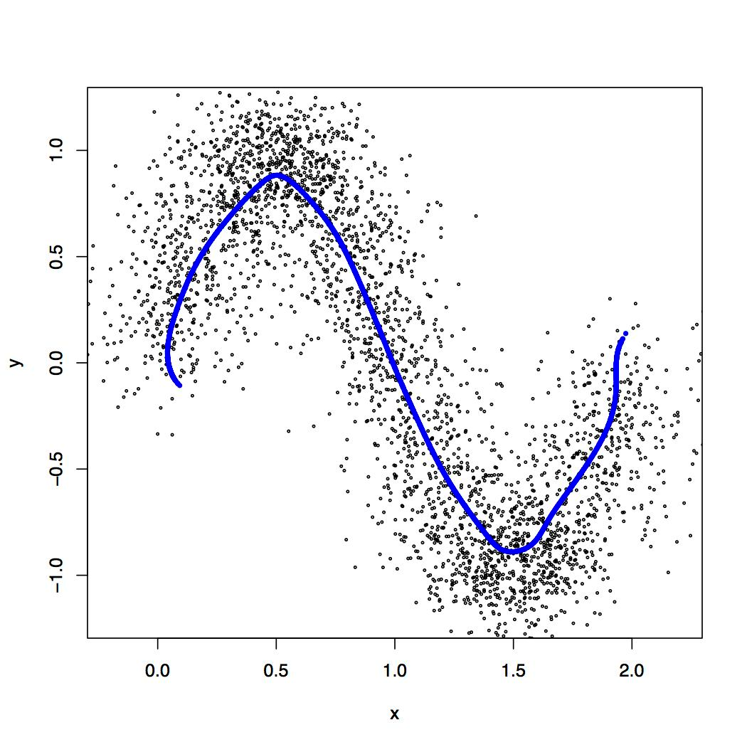
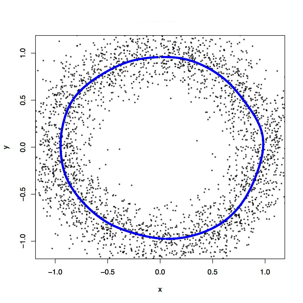
Consider point-cloud data in , drawn independently from a density with compact support. We define the filaments of the data distribution as the ridges of the probability density function . (See Section 2.1 for details.) There are several alternative ways to formally define filaments [Eberly (1996)], but the definition we use has several useful statistical properties [Genovese et al. (2012d)]. Figure 1 shows two simple examples of point cloud data sets and the filaments estimated by our method.
The problem of estimating filaments has been studied in several fields and a variety of methods have been developed, including parametric [Stoica et al. (2007), Stoica et al. (2008)]; nonparametric [Genovese et al. (2012b), Genovese et al. (2012a), Genovese et al. (2012c)]; gradient based [Genovese et al. (2012d), Sousbie (2011), Novikov et al. (2006)]; and topological [Dey (2006), Lee (1999), Cheng et al. (2005), Aanjaneya et al. (2012), Lecci et al. (2013)].
While all these methods provide filament estimates, none provide an assessment of the estimate’s uncertainty. That filament estimates are random sets is a significant challenge in constructing valid uncertainty measures [Molchanov (2005)]. In this paper, we introduce a local uncertainty measure for filament estimates. We characterize the asymptotic distribution of estimated filaments and use it to derive consistent estimates of the local uncertainty measure and to construct valid confidence sets for the filament based on bootstrap resampling. Our main results are as follows:
-
•
We show that if the data distribution is smooth, so are the estimated filaments (Theorem 1).
- •
-
•
We construct valid and consistent, bootstrap confidence sets for the local uncertainty, and thus pointwise confidence sets for the filament (Theorem 6).
We apply our methods to point cloud data from examples in Astronomy and Seismology and demonstrate that they yield useful confidence sets.
2 Background
2.1 Density Ridges
Let be random sample from a distribution with compact support in that has density . Let and denote the gradient and Hessian, respectively, of . We begin by defining the ridges of , as defined in [Genovese et al. (2012d), Ozertem and Erdogmus (2011), Eberly (1996)]. While there are many possible definitions of ridges, this definition gives stability in the underlying density, estimability at a good rate of convergence, and fast reconstruction algorithms, as described in [Genovese et al. (2012d)]. In the rest of this paper, the filaments to be estimated are just the one-dimensional ridges of .
A mode of the density – where the gradient is zero and all the eigenvalues of are negative – can be viewed as a zero-dimensional ridge. Ridges of dimension generalize this to the zeros of a projected gradient where the smallest eigenvalues of are negative. In particular for ,
| (1) |
where
| (2) |
is the projected gradient. Here, the matrix is defined as for eigenvectors of corresponding to eigenvalues Because one-dimensional ridges are the primary concern of this paper, we will refer to in (1) as the “ridges” of .
Intuitively, at points on the ridge, the gradient is the same as the largest eigenvector and the density curves downward sharply in directions orthogonal to that. When is smooth and the eigengap is positive, the ridges have the all essential properties of filaments. That is, decomposes into a set of smooth curve-like structures with high density and connectivity. can also be characterized through Morse theory [Guest (2001)] as the collection of -critical-points along with the local maxima, also known as the set of 1-ascending manifolds with their local-maxima limit points [Sousbie (2011)].
2.2 Ridge Estimation
We estimate the ridge in three steps: density estimation, thresholding, and ascent. First, we estimate from from the data . Here, we use the well-known kernel density estimator (KDE) defined by
| (3) |
where the kernel is a smooth, symmetric density function such as a Gaussian and is the bandwidth which controls the smoothness of the estimator. Because ridge estimation can tolerate a fair degree of oversmoothing (as shown in [Genovese et al. (2012d)]), we select by a simple rule that tends to oversmooth somewhat, the multivariate Silverman’s rule [Silverman (1986)]. Under weak conditions, this estimator is consistent; specifically, as . (We say that converges in probability to , written if, for every , as .)
Second, we threshold the estimated density to eliminate low-probability regions and the spurious ridges produced in by random fluctuations. Here, we remove points with estimated density less than for a user-chosen threshold .
Finally, for a set of points above the density threshold, we follow the ascent lines of the projected gradient to the ridge, which is the the subspace constrainted mean shift (SCMS) algorithm [Ozertem and Erdogmus (2011)]. This procedure can be viewed as estimating the ridge by applying the Ridge operator to :
| (4) |
Note that is a random set.
2.3 Bootstrapping and Smooth Bootstrapping
The bootstrap [Efron (1979)] is a statistical method for assessing the variability of an estimator. Let be a random sample from a distribution and let be some functional of to be estimated, such as the mean of the distribution or (in our case) the ridge set of its density. Given some procedure for estimating we estimate the variability of by resampling from the original data.
Specifically, we draw a bootstrap sample independently and with replacement from the set of observed data points and compute the estimate using the bootstrap sample as if it were the data set.
This process is repeated times, yielding bootstrap samples and corresponding estimates . The variability in these estimates is then used to assess the variability in the original estimate . For instance, if is a scalar, the variance of is estimated by
where . Under suitable conditions, it can be shown that this bootstrap variance estimates – and confidence sets produced from it – are consistent.
The smooth bootstrap is a variant of the bootstrap that can be useful in function estimation problems where the same procedure is used except the bootstrap sample is drawn from the estimated density instead of the original data. We use both variants below.
3 Methods
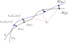
We measure the local uncertainty in a filament (ridge) estimator by the expected distance between a specified point in the original filament and the estimated filament:
| (5) |
where is the distance function:
| (6) |
The local uncertainty measure can be understood as the expected dispersion for a given point in the original filament to the estimated filament based on sample with size . The theoretical analysis of is given in theorem 5.
3.1 Estimating Local Uncertainty
Because is defined in terms unknown distribution and the unknown filament set , it must be estimated. We use bootstrap resampling to do this, defining an estimate of local uncertainty on the estimated filaments. For each of bootstrap samples, , we compute the kernel density estimator , the ridge estimate , and the divergence for all . We estimate by
| (7) |
for each , where the expectation is from the (known) bootstrap distribution. Algorithm 1 provides pseudo-code for this procedure, and Theorem 6 shows that the estimate is consistent under smooth bootstrapping.
3.2 Pointwise Confidence Sets
Confidence sets provide another useful assessment of uncertainty. A confidence set is a random set computed from the data that contains an unknown quantity with at least probability . We can construct a pointwise confidence set for filaments from the distance function (6). For each point , let be the quantile value of from the bootstrap. Then, define
| (8) |
This confidence set capture the local uncertainty: for a point with low (high) local uncertainty, the associated radius is small (large). But note that the confidence set attains coverage around each point; the coverage of the entire filament set is lower. That is, we can have high probability to cover each point but the probability to simultaneously cover all points (the whole filament set) might be lower.
4 Theoretical analysis
For the filament set , we assume that it can be decomposed into a finite partition
such that each is a one dimensional manifold. Such a partition can be constructed by the equation of traversal in page 56 of [Eberly (1996)]. For each , we can parametrize it by a function from the equation of traversal mentioned with suitable scaling.
For simplicity, in the following proofs we assume that the filament set is a single so that we can construct the parametrization easily. All theorems and lemmas we prove can be applied to the whole filament set by repeating the process for each individual .
4.1 Smoothness of Density Ridges
To study the properties of the uncertainty estimator, we first need to establish some results about the smoothness of the filament. The following theorem provides conditions for smoothness of the filaments. Let denote the collection of times continuously differentiable functions.
Theorem 1 (Smoothness of Filaments)
Let be a parameterization of filament set , and for , let be an open set containing . If is and the eigengap for , then is for .
Theorem 1 says that filaments from a smooth density will be smooth. Moreover, estimated filaments from the KDE will be smooth if the kernel function is smooth. In particular, if we use Gaussian kernel, which is , then the corresponding filaments will be as well.
4.2 Frenet Frame

In the arguments that follow, it is useful to have a well-defined “moving” coordinate system along a smooth curve. Let be an arc-length parametrization for a curve with . The Frenet frame [Kuhnel (2002)] along is a smooth family of orthogonal bases at
such that determines the direction of the curve. The other basis elements are called the curvature vectors and can be determined by a Gram-Schmidt construction.
Assume the density is . We can construct a Frenet frame for each point on the filaments. Let be the Frenet frame of such that
where is the th derivative of the and is the inner product of vector . An important fact is that the basis element is , . Frenet frames are widely used in dynamical systems because they provide a unique and continuous frame to describe trajectories.
4.3 Normal space and distance measure
The reach of , denoted by , is the smallest real number such that each has a unique projection onto [Federer (1959)].
We define the normal space of by
| (9) |
Note that since we have second derivative of exists and finite, the reach will be bounded from below.
Finally, define the Hausdorff distance between two subsets of by
| (10) |
where and .
4.4 Local uncertainty
Let the estimated filament be the ridge of KDE. We assume the following:
-
(K1)
The kernel is .
-
(K2)
The kernel satisfies condition in page 5 of [Gine and Guillou (2002)].
-
(P1)
The true density is in .
-
(P2)
The ridges of have positive reach.
-
(P3)
The ridges of are closed. For example, Figure 1-(b).
(K1) and (K2) are very mild assumptions on the kernel function. For instance, Gaussain kernels satisfy both. (P1-P3) are assumptions on the true density. (P1) is a smoothness condition. (P2) is a smoothness assumption on the ridge. (P3) is included to avoid boundary bias when estimating the filament near endpoints.
Now we introduce some norms and semi-norms characterizing the smoothness of the density . A vector of non-negative integers is called a multi-index with and corresponding derivative operator
where is often written as . For , define
| (11) |
When , we have the infinity norm of ; for , these are semi-norms. We also define
| (12) |
It is easy to verify that this is a norm. Next we recall a theorem in [Genovese et al. (2012d)] which establish the link of Hausdorff distance between with the metric between density.
Theorem 2 (Theorem 6 in [Genovese et al. (2012d)])
Under conditions in [Genovese et al. (2012d)], as is sufficiently small , we have
This theorem tells us that we have convergence in Hausdorff distance for estimated filaments.
Lemma 3 (Local parametrization)
For the estimated filament , define and . Assume (K1), (K2), (P1), (P2). If , then, when is sufficiently small,
-
1.
is a singleton for all except in a set containing the boundaries with .
-
2.
for not at the boundary of filaments.
-
3.
If in addition (P3) holds, then .
Claim 1 follows because the Hausdorff distance is less than . This will be true since by Theorem 2, the Hausdorff distance is contolled by , and we have a stronger convergence assumption. The only exception is points near the boundaries of since can be shorter than in this case. But this can only occur in the set with length less than Hausdorff distance. Claim 2 follows from the fact that the normal space for and will be asymptotically the same. If we assume (P3), then has no boundary, so that is an empty set.
Note that Claim 2 gives us the validity of approximation for via . So the limiting bahavior of local uncertainty will be the same as . In the following, we will study the limiting distributions for .
We define the subspace derivative by , which in turn gives the subspace gradient
and the subspace Hessian
Then we have the following theorem on local uncertainty, where denotes convergence in distribution.
Theorem 4 (Local uncertainty theorem)
Assume (K1),(K2),(P1),(P2). If , then
where
for all with .
Theorem 4 states the asymptotic behavior of which is asymptotically equivalent to local uncertainty. is the bias component and is the stochastic variation component in which the parameter controls the amount of varitaion. The contents in parameters and link the geometry of the local density function with the local uncertainty.
Remarks:
-
•
Note that is a sufficient condition for up to the fourth derivative uniform convergence. The uniform convegence in these derivative along with (P2) and theorem 1 ensures the reach of will converge to the condition number of .
By theorem 4 and claim 2 in lemma 3, we know the asymptotic distribution of local uncertainty . So we have the following theorem on local uncertainty measure.
Theorem 5
Define the local uncertatiny measure by
where ranges over all points in . Assume that (K1), (K2), (P1), and (P2) hold. If then
for all with .
4.5 Bootstrapping Result
For the bootstrapping result, we assume (P3) for convenience. Note that if we do not assume (P3), the result still holds for points not close to terminals. Let be a sequence of densities satisfying (P1). We want to study the local uncertainty of the associated filaments. So we work on the random sample generated from and use the random sample to build estimated filaments for filaments of . Define as the a parametrization for the filaments and associated normal space of . Then we have the following convergence theorem for a sequence of densities converging to .
Theorem 6
Assume that (P1–3) hold. Let be a sequence of probability densities that satisfy (P1), (P2), and as .
If is sufficiently small, we can find a bijection such that
-
1.
.
-
2.
.
-
3.
.
-
4.
.
In particular, if we use with , then the above result holds with high probability.
Note that the local uncertainty measure has unknown support and unknown parameters given in theorem 5. Claim 1 shows the convergence in support while claim 3,4 prove the consistency of the parameters controlling uncertainties. This theorem states that if we have a sequence of densities converging to a limiting density, then the local uncertainty will converge in a sense.
Remarks:
-
•
Notice that need not be the same as . The latter one lives in the normal space of but the former need only be a continuously bijective mapping. The projection that maps to the point is one choice of .
-
•
The last result holds immediately from Lemma 8 as we pick . The bandwidth in this case will ensure uniform convergence in probability up to the forth derivative which is sufficient to the condition.
5 Examples
We apply our methods to two datasets, one from astronomy and one from seismology. In both cases, we use an isotropic Gaussian kernel for the KDE and threshold using . We use a uniform grid over each sample as initial points in the ascent step for running SCMS. We compare the result from bootstrapping and smooth bootstrapping based on 100 bootstrap samples to estimate uncertainty.
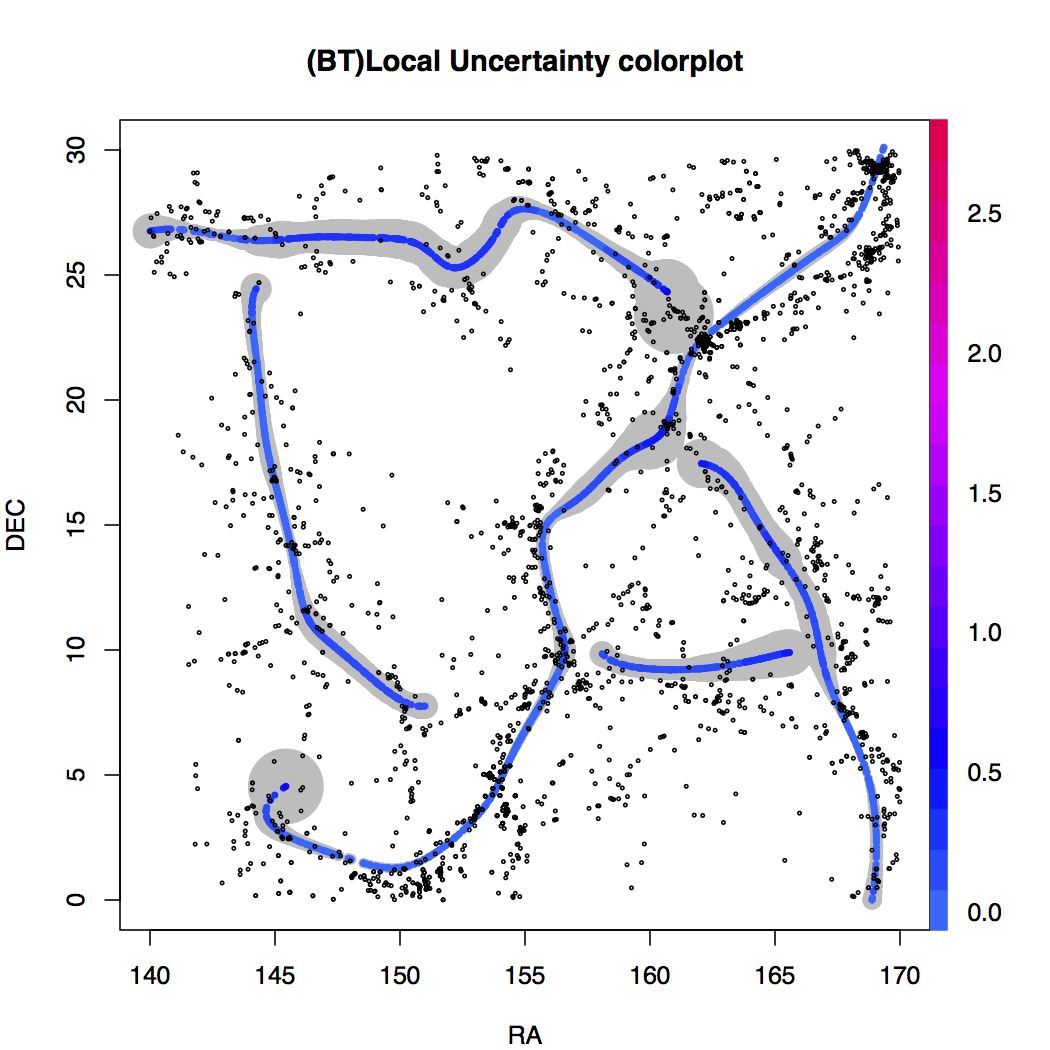
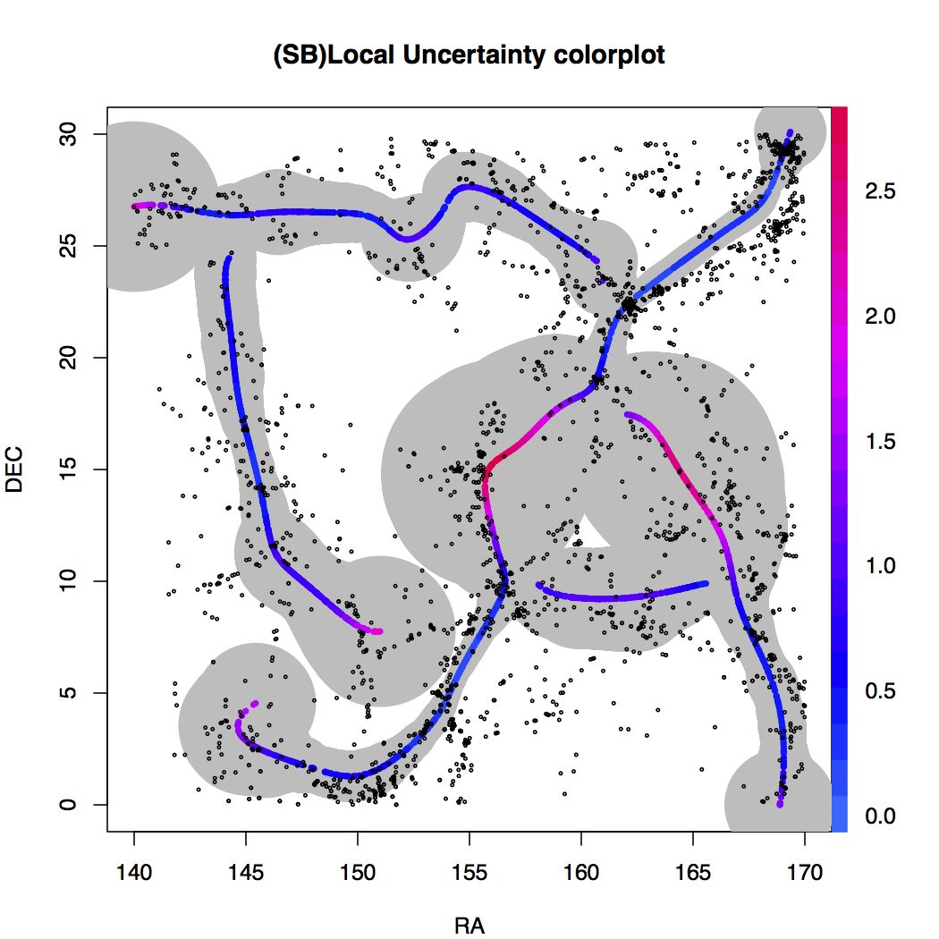
Astronomy Data. The data come from Sloan Digit Sky Survey(SDSS) Data Release(DR) 9. 111The SDSS dataset http://www.sdss3.org/dr9/ In this dataset, each point is a galaxy and is characterized by three features (z, ra, dec). z is the redshift value, a measurement of the distance form that galaxy to us. ra is right ascesion, the latitude of the sky. dec is declination, the longitude of the sky.
We restrict ourselves to z=0.0450.050 which is a slice of data on the z coordinate that consists of galaxies. We selected values in (ra, dec)=(0 30, 140 170). The bandwidth is 2.41.
Figure 6 displays the local uncertainty measures with pointwise confidence sets. The red color indicates higher local uncertainty while the blue color stands for lower uncertianty. Bootstrapping shows a very small local uncertainty and very narrow pointwise confidence sets. Smooth bootstapping yields a loose confidence sets but it shows a clear pattern of local uncertainty which can be explained by our theorems.
From Figure 6, we identify four cases associated with high local uncertainty: high curvature of the filament, flat density near filaments, terminals (boundaries) of filaments, and intersecting of filaments. For the points near curved filaments, we can see uncertainty increases in every case. This can be explained by theorem 4. The curvature is related to the third derivative of density from the definition of ridges. From theorem 4, we know the bias in filament estimation is proportional to the third derivative. So the estimation for highly curved filaments tends to have a systematic bias in filament estimation and our uncertainty measure captures this bias successfully.
For the case of a flat density, by theorem 4, we know both the bias and variance of local uncertainty is proportional to the inverse of the Hessian. A flat density has a very small Hessian matrix and thus the inverse will be huge; this raises the uncertainty. Though our theorem can not be applied to terminals of filaments, we can still explain the high uncertianty. Points near terminals suffer from boundary bias in density estimation. This leads to an increase in the uncertainty. For regions near connections, the eigengap will approach which causes instability of the ridge since our definition of ridge requires . All cases with high local uncertainty can be explained by our theoretical result. So the data analysis is consistent with our theory.
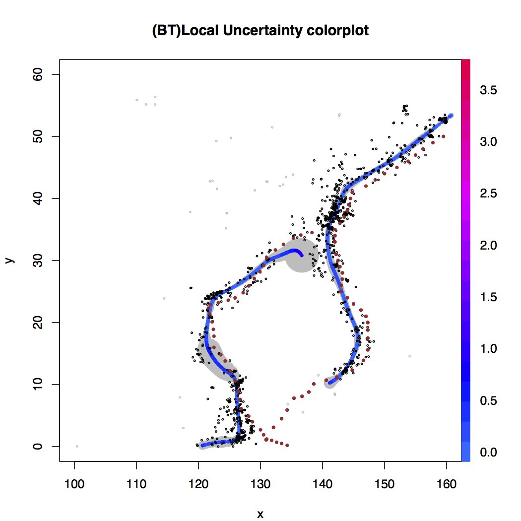
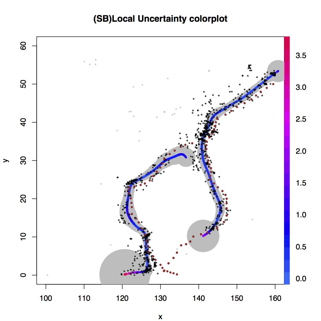
Earthquake Data. We also apply our technique to data from the U.S. Geological Survey 222The USGS dataset http://earthquake.usgs.gov/earthquakes/search/ that locates earthquakes hat occur in region between longitude , latitude and in dates between 01/01/2013 to 09/30/2013. We are particularly interested in detecting plate boundaries, which see a high incidence of earthquakes. We pre-process the data to remove a cluster of earthquakes that are irrelevant to the plate boundary. For this data, we only consider those filaments with density larger than of the maximum of the density. Because the noise level is small, we adjust the KDE bandwidth to times the Silverman rule ().
Figure 7 displays the estimated filaments and pointwise confidence sets. The Figure shows the true plate boundaries from Nuvel data set 333Nuvel data set http://www.earthbyte.org/ as brown points. As can be seen in the Figure, smooth bootstrapping has better coverage over the plate boundary. We notice the bad coverage in the bottom part; this is reasonable since the boundary bias and lack of data cause trouble in estimation and uncertainty measures. We also identify some parts of filaments with high local uncertainty. The filaments with high uncertainty can be explained by theorem 4. The data analysis again support our theoretical result.
In both Figure 6, 7, we see a clear picture on the uncertainty assessment for filament estimation. In data from two or three dimension, we can visualize uncertainties in estimation of filaments with different colors or confidence regions. That is, we can display estimation and the uncertainty in the same plot.
6 Discussion and Future Work
In this paper, we define a local uncertainty measure for filament estimation and study its theoretical properties. We apply bootstrap resampling to estimate local uncertainty measures and construct confidence sets, and we prove that both are consistent and data analysis also supports our result. Our method provides one way to numerically quantify the uncertainty for estimating filaments. We also visualize uncertatiny measures with estimated filaments in the same plot; this can be one easy way to show estimation and the uncertainty simultaneously.
Our approach has no constraints on the dimension of the data so it can be extended to data from higher dimension (although the confidence sets will be larger). Our definition of local uncertainty and our estimation method can be applied to other geometric estimation algorithms, which we will investigate in the future.
Appendix A Proofs
Proof A.1 ( of Theorem 1).
For the ridge set , it is a collection of solutions to as the eigengap . But is a orthonormal basis. So the solution to is equal to the solution to . Now . Hence, implicit function theorem tells us that the differentiablilty of a local graph is the same as when . Now since the local graph is parametrized by one variable, we can reparametrize it by a curve . And the differentiability of the curve is the same as .
From a slight modification from theorem 3 in [Genovese et al. (2012d)], the th order derivative of depends on th order derivative of density if the eigengap . Hence, if the density is and we consider an open set with , then we have is on so the result follows.
To prove theorem 4, we need the following lemmas:
Lemma 7.
Let be KDE for . Assume our kernel satisfies (K1), (K2). If . Then admits an asymptotic normal distribution by
| (13) |
where
| (14) | ||||
| (15) |
is the kernel used and is a constant of kernel.
Proof A.2.
For KDE ,
| (16) |
Hence for ,
Notice that each is independent and identically distributed.
We will show that satisfies conditions for Lyapounov’s condition so that we have Central Limit Theorem (CLT) result for it. WLOG, we consider the third moment and focus on partial derivative over a direction, say , we want
| (17) |
where .
This is equivalent to show
| (18) |
Now we put an upper bound on (18), then we have
We assume that for all . Therefore by Taylor expansion over density and take the first order, we have
As a result, Lyapounov’s condition is satisfied and this holds for all ; so we have CLT for .
By multivariate CLT we have
where is the identity matrix of dimension .
By theorem 4 in [Chacón et al. (2011)], we have
Therefore, as and ,
Now since so tends to 0 and multiply in both side, we get
This completes the proof.
Lemma 8.
([Gine and Guillou (2002)]; version of [Genovese et al. (2012d)])
Assume (K1), (P1) and the kernel function satisfies conditions in [Gine and Guillou (2002)]. Then we have
| (19) |
Lemma 9.
For a density , let be its filaments. For any points on , let the Hessian at be with eigenvectors and eigenvalues . Consider any subspace spanned by a basis with be the normal vector for . Then a sufficient and necessary condition for be a local mode of constrained in is
| (20) |
A sufficient condition for (20) is
| (21) |
Proof A.3.
Let the Hessian of density at be with eigenvectors and associated eigenvalues . Consider any subspace spanned by a basis with be the normal vector for
For any on the ridge, we have . is the mode constrained in the subspace if is negative definite. By spectral decomposition, we can write
where and is a diagonal matrix of eigenvalues. So this matrix will be negative definite if and only if all its diagonoal elements are negative.
That is, the sufficient and necessary condition is
| (22) |
We explicitly derive the form of (22) and consider the sufficient and necessary condition:
So we prove the first condition.
To see the sufficient condition, we note that by definition, . So for each ,
This implies that for each ,
Note that we use the fact since and ’s are basis.
Since both and are basis, we have
for all . Then we further have
for each .
Putting altogether, we have
for all
So a sufficient condition is
Proof A.4 ( of Theorem 4).
By definition of and the nature of ridge, is the local mode of in the subspace spanned by near . By lemma 9, will also the local mode of in the subspace spanned by near once the two filamnets are closed enough and the local direction of filaments are also closed. This will be shown in 2. of theorem 6.
Hence, we have
Now applying Taylor expansion for near , we have
where is the projected Hessian of KDE while , for some .
Accordingly,
| (23) |
By lemma 8 with and we pick a suitable , we have
which implies
and will converge to . Consequently,
This implies
| (24) |
since is non-singular.
Hence, for the subspace case:
| (25) |
Now since always lays in the subspace , we have
Proof A.5 ( of Theorem 6).
1. By assumption, the ridges for and have positive conditioning number. We can apply theorem 6. in Genovese et. al. (2012) so that and will be asymptotically topological homotopy. So we can always find a continuous bijective mapping to map every point on to . We define be such a map on each point of . Since the Hausdorff distance converge to , the associated mapping can be picked such that each pair has distance less than Hausdorff distance. So the result follows.
2. Recall that filaments are solutions to
The direction of ridge () depends on up to third derivative at points on the filaments. From 1., we know that the location of will converge to and we have the uniform convergence up to the third derivative by assumptions. Hence, by uniformly convergence and both are , we have convergence in the tangent line at each point of filaments. So this implies the inner product to be 1.
3. From theorem 4, . By assumption, we have uniform convergence up to third derivative and by 2. we have convergence in subspace. So from will unifromly converge to that from .
4. Similar to 3.
References
- [1]
- Aanjaneya et al. (2012) Mridul Aanjaneya, Frederic Chazal, Daniel Chen, Marc Glisse, Leonidas Guibas, and Dmitriy Morozov. 2012. Metric graph reconstruction from noisy data. International Journal of Computational Geometry and and Applications (2012).
- Bond et al. (1996) J. R. Bond, L. Kofman, and D. Pogosyan. 1996. How filaments of galaxies are woven into the cosmic web. Nature (1996).
- Chacón et al. (2011) J.E. Chacón, T. Duong, and M.P Wand. 2011. Asymptotics for general multivariate kernel density derivative estimators. Statistica Sinica (2011).
- Cheng et al. (2005) S.-W. Cheng, S. Funke, M. Golin, P. Kumar, S.-H. Poon, and E. Ramos. 2005. Curve reconstruction from noisy samples. In Computational Geometry 31.
- Dey (2006) T. Dey. 2006. Curve and Surface Reconstruction: Algorithms with Mathematical Analysis. Cambridge University Press.
- Eberly (1996) David Eberly. 1996. Ridges in Image and Data Analysis. Springer.
- Efron (1979) B. Efron. 1979. Bootstrap Methods: Another Look at the Jackknife. Annals of Statistics 7, 1 (1979), 1–26.
- Federer (1959) H. Federer. 1959. Curvature measures. Trans. Am. Math. Soc 93 (1959).
- Genovese et al. (2012a) Christopher R. Genovese, Marco Perone-Pacifico, Isabella Verdinelli, and Larry Wasserman. 2012a. The geometry of nonparametric filament estimation. J. Amer. Statist. Assoc. (2012).
- Genovese et al. (2012b) Christopher R. Genovese, Marco Perone-Pacifico, Isabella Verdinelli, and Larry Wasserman. 2012b. Manifold estimation and singular deconvolution under hausdorff loss. The Annals of Statistics (2012).
- Genovese et al. (2012c) Christopher R. Genovese, Marco Perone-Pacifico, Isabella Verdinelli, and Larry Wasserman. 2012c. Minimax manifold estimation. Journal of Machine Learning Research (2012).
- Genovese et al. (2012d) Christopher R. Genovese, Marco Perone-Pacifico, Isabella Verdinelli, and Larry Wasserman. 2012d. Nonparametric ridge estimation. arXiv:1212.5156v1 (2012).
- Gine and Guillou (2002) E. Gine and A Guillou. 2002. Rates of strong uniform consistency for multivariate kernel density estimators. In Annales de l’Institut Henri Poincare (B) Probability and Statistics (2002).
- Guest (2001) Martin A. Guest. 2001. Morse theory in the 1990’s. arXiv:math/0104155v1 (2001).
- Hile et al. (2009) Harlan Hile, Radek Grzeszczuk, Alan Liu, Ramakrishna Vedantham, Jana Košecka, and Gaetano Borriello. 2009. Landmark-Based Pedestrian Navigation with Enhanced Spatial Reasoning. Lecture Notes in Computer Science 5538 (2009).
- Kuhnel (2002) Wolfgang Kuhnel. 2002. Differential geometry: curves-surfaces-manifolds. Vol. 16. student mathematical library.
- Lalonde and Strazielle (2003) R. Lalonde and C. Strazielle. 2003. Neurobehavioral characteristics of mice with modified intermediate filament genes. Rev Neurosci (2003).
- Lecci et al. (2013) Fabrizio Lecci, Alessandro Rinaldo, and Larry Wasserman. 2013. Statistical Analysis of Metric Graph Reconstruction. arXiv:1305.1212 (2013).
- Lee (1999) I.-K. Lee. 1999. Curve reconstruction from unorganized points.. In Computer Aided Geometric Design 17.
- Molchanov (2005) I. Molchanov. 2005. Theory of random sets. Springer-Verlag London Ltd.
- Novikov et al. (2006) D. Novikov, S. Colombi, and O. Dore. 2006. Skeleton as a probe of the cosmic web: the two-dimensional case. Mon. Not. R. Astron. Soc. (2006).
- Ozertem and Erdogmus (2011) Umut Ozertem and Deniz Erdogmus. 2011. Locally Defined Principal Curves and Surfaces. Journal of Machine Learning Research (2011).
- Silverman (1986) B. W Silverman. 1986. Density Estimation for Statistics and Data Analysis. Chapman and Hall.
- Sousbie (2011) T. Sousbie. 2011. The persistent cosmic web and its filamentary structure – I. Theory and implementation. Mon. Not. R. Astron. Soc. (2011).
- Stoica et al. (2007) R. Stoica, V. Martinez, and E. Saar. 2007. A three-dimensional object point process for detection of cosmic filaments. Appl. Statist. (2007).
- Stoica et al. (2008) R. S. Stoica, V. J. Mart́ınez, J. Mateu, and E. Saar. 2008. Detection of cosmic filaments using the Candy model. A. and A. (2008).
- USGS (2003) USGS. 2003. Where are the Fault Lines in the United States East of the Rocky Mountains?