Blind Identification via Lifting

Abstract

Blind system identification is known to be an ill-posed problem and without further assumptions, no unique solution is at hand. In this contribution, we are concerned with the task of identifying an ARX model from only output measurements. We phrase this as a constrained rank minimization problem and present a relaxed convex formulation to approximate its solution. To make the problem well posed we assume that the sought input lies in some known linear subspace.

1 Introduction

Consider an auto-regressive exogenous input (ARX) model

$$y(t)- a_{1}y(t-1)-\cdots-a_{n_{a}}y(t-n_{a})$$

$$= {b}_{1}u(t-n_{k}-1)+\cdots+{b}_{n_{b}}u(t-n_{k}-n_{b})$$ (1)

with input $u\in{\mathbb{R}}$ and output $y\in{\mathbb{R}}$. Estimation of this type of model is one of the most common tasks in system identification and a very well studied problem, see for instance Ljung (1999). The common setting is that $\{(y(t),u(t))\}_{t=1}^{N}$ is given and the summed residuals

$$\sum_{t=n}^{N}\left(y(t)-\sum_{k_{1}=1}^{n_{b}}{b}_{k_{1}}u(t-k_{1}-n_{k})-\sum_{k_{2}=1}^{n_{a}}a_{k_{2}}y(t-k_{2})\right)^{2}$$

where $n=\max(n_{a},n_{k}+n_{b})+1$, is minimized to obtain an estimate for $a_{1},\dots,a_{n_{a}},{b}_{1},\dots,{b}_{n_{b}}$. This estimate is often referred to as the least squares (LS) estimate.

In this paper we study the more complicated problem of estimating an ARX model from solely outputs $\{y(t)\}_{t=1}^{N}$. This is an ill-posed problem and it is easy to see that under no further assumptions, it would be impossible to uniquely determine $a_{1},\dots,a_{n_{a}},{b}_{1},\dots,{b}_{n_{b}}$. We will here therefore study this problem under the assumption that the stacked inputs belong to some known subspace. The input could for example be:

• known to change only at a set of discrete times due to a discrete controller or

• known to be band-limited and therefore well represented by the projection on the first discrete Fourier transform basis vectors.

It should be noticed that this assumption is not enough to uniquely determine the input or the ARX model. Specifically, we will not be able to decide the input or the ARX coefficients ${b}_{1},\dots,{b}_{n_{b}}$ more than up to a multiplicative scalar. It should be stressed that this is not a limitation of the method that we propose but an inherent limitation of the system identification problem since the sought quantities always appear as products. To uniquely determine the input and the ARX coefficients ${b}_{1},\dots,{b}_{n_{b}}$, further knowledge is needed.

The main contribution of the paper is a novel method for ARX model identification from only output measurements. The method takes the form of a convex optimization problem and gives a computationally flexible framework for handling different types of measurement noises, constraints, etc.

2 Background

Blind system identifican (BSI) has a broad application area and has been applied in fields such as data communications, speech recognition and seismic signal processing, see for instance Abed-Meraim et al. (1997). Common for the type of modeling problems that BSI has been applied to is that the input is difficult, costly or impossible to measure. In for example exploration seismology, the physical properties of the earth are explored by studying the response of an excitation (often a charge of dynamite). The excitation is often difficult to measure and the modeling problem therefore a BSI problem, see e.g., Zerva et al. (1999).

Many methods have been proposed to solve the BSI problem throughout the years. We give a short overview here but refer the interested reader to Abed-Meraim et al. (1997); Hua (2002), for a more extensive and complete review.

The maximum likelihood (ML) approach to BSI aims at finding the ML estimate of the model and input. The resulting non-convex optimization problem is often treated by alternating between optimizing with respect to the input and the system model. See Abed-Meraim and Moulines (1994). The channel subspace (CS) methods to BSI indirectly determine the sought finite impulse response (FIR) model by estimating the nullspace of the Sylvester matrix associated with the FIR model to be identified. This is done by an eigen decomposition of a matrix derived from the outputs. See for instance Abed-Meraim et al. (2006). The method proposed in Zerva et al. (2000) works under the assumption that two or more output series are available and that these were generated by the same input. See also Van Vaerenbergh et al. (2013). The methods proposed in Sato (1975); Tong et al. (1991) assume that the input consists of independent and identically (iid) distributed random variables and considers the autocorrelation of the output to decide a FIR model and the unknown input.

A number of approaches consider the blind identification problem of Hammerstein systems under the assumption that the input is piecewise constant. Sun et al. (1999); Bai et al. (2010); Bai and Fu (2002); Wang et al. (2007, 2009, 2010). Our approach assumes that the input belongs to some known subspace. Piecewise constant signal can be represented using the subspace assumption used here. However, we note that we are not restricted to piecewise constant signals, and our approach is significantly different. Also, we consider the blind identification of ARX models while the blind identification problem of Hammerstein systems is considered in Sun et al. (1999); Bai et al. (2010); Bai and Fu (2002); Wang et al. (2007, 2009, 2010).

The related problem of blind deconvolution have been studied in a number of contributions. In particular, see the very interesting paper by Ahmed et al. (2012) for a solution where the signals to be recovered are assumed to be in some known subspaces. The development presented in Ahmed et al. (2012) has similarities to the approach presented in this paper and was done in parellel to our work. Note that only FIR models are discussed in Ahmed et al. (2012) and that the analysis does not apply.

3 Problem Formulation

Given the sequence of outputs $\{y(t)\}_{t=1}^{N}\in{\mathbb{R}}$, find an estimate for $a_{1},\dots,a_{n_{a}},{b}_{1},\dots,{b}_{n_{b}}\in{\mathbb{R}}$ and $u(t)\in{\mathbb{R}},t=1,\dots,N,$ such that

$$y(t)- a_{1}y(t-1)-\cdots-a_{n_{a}}y(t-n_{a})$$

$$= {b}_{1}u(t-n_{k}-1)+\cdots+{b}_{n_{b}}u(t-n_{k}-n_{b})+w(t),$$

for $t=n,\dots,N$, where $n=\max(n_{a},n_{k}+n_{b})+1$, and $w(t),\,t=n,\dots,N$, some unknown zero mean noise. We will for simplicity assume that $n_{a},n_{b},n_{k},$ are known. To make the problem well posed, we will seek an input in a given subspace of ${\mathbb{R}}^{N}$.

4 Notation and Assumptions

We will use $y$ to denote the output and $u$ the input. We will for simplicity only consider single input single output (SISO) systems, however with some extra bookkeeping also MIMO systems could be treated. We will assume that $N$ measurements of $y$ are available and stack them in the vector ${\bf y}$, i.e.,

$${\bf y}=\begin{bmatrix}{y}(1)&\dots&{y}(N)\end{bmatrix}^{\mathsf{T}}.$$ (2)

We also introduce ${\bf u}$, $\eta$, ${\bf a}$ and ${\bf b}$ as

$${\bf u}= \begin{bmatrix}u(1)&\dots&u(N)\end{bmatrix}^{\mathsf{T}},$$ (3)

$${\eta}= \begin{bmatrix}\eta(1)&\dots&\eta(N)\end{bmatrix}^{\mathsf{T}},$$ (4)

$${\bf a}= \begin{bmatrix}a_{1}&\dots&a_{n_{a}}\end{bmatrix}^{\mathsf{T}},$$ (5)

$${\bf b}= \begin{bmatrix}{b}_{1}&\dots&{b}_{n_{b}}\end{bmatrix}^{\mathsf{T}}.$$ (6)

We will use ${\bf y}(i)$ to denote the $i$th element of ${\bf y}$. To pick out a subvector of ${\bf y}$ consisting of the $i$th to the $j$th element we will use the notation ${\bf y}(i:j)$ and similarly for picking out a subvector of ${\bf u}$, ${\bf a}$ and ${\bf b}$. To pick out a submatrix consisting of the $i$th to the $j$th rows of ${\bf X}$ we use the notation ${\bf X}(i:j,:)$. We will use normal font to represent scalars and bold for vectors and matrices. $\|\cdot\|_{0}$ is the zero (quasi) norm which returns the number of nonzero elements of its argument and $\|\cdot\|_{*}$ the nuclear norm returning the sum of the singular values.

We will assume that it is known that the sought input, ${\bf u}$, lies in some known subspace. We can hence write

$${\bf u}={\bf D}{\bf x}$$ (7)

for some known $N\times m$-matrix ${\bf D}$ and an unknown vector ${\bf x}\in{\mathbb{R}}^{m}$. It is assumed that $m\leq N$.

5 Blind Identification via Lifting

Consider the noise free setting where $w(t)=0,\,t=n,\dots,N.$ We can formulate the problem of finding an input and the ARX coefficients as the feasibility problem

$$\text{find}_{\begin{array}[]{cc}u(t),\,t=1,\dots,N,\\ a_{1},\dots,a_{n_{a}},{b}_{1},\dots,{b}_{n_{b}}\end{array}}\quad$$ (8c)

$${\mbox{subj. to}}\quad y(t)- \sum_{k_{2}=1}^{n_{a}}a_{k_{2}}y(t-k_{2})$$

$$= \sum_{k_{1}=1}^{n_{b}}{b}_{k_{1}}u(t-n_{k}-k_{1}),\quad t=n,\dots,N.$$ (8d)

Note that the $\{a_{k}\}_{k=1}^{n_{a}}$, $\{{b}_{k}\}_{k=1}^{n_{b}}$, and $\{u(t)\}_{t=1}^{N}$ are unknown. The problem is therefore non-convex.

Introduce ${\bf X}={\bf x}{\bf b}^{\mathsf{T}}\in{\mathbb{R}}^{m\times n_{b}}$ and note that (7) gives that ${\bf D}{\bf X}={\bf D}{\bf x}{\bf b}^{\mathsf{T}}={\bf u}{\bf b}^{\mathsf{T}}$. Since ${\bf u}{\bf b}^{\mathsf{T}}$ contains all products $u(i)b_{j},\,i=1,\dots,N,\,j=1,\dots,n_{b}$, the sum

$$\sum_{k_{1}=1}^{n_{b}}{b}_{k_{1}}u(t-n_{k}-k_{1})$$ (9)

can be realized by summing appropriate entries of ${\bf D}{\bf X}$. Problem (8) can now be reformulated as

$$\text{find}_{{\bf X},{\bf a}}\quad$$ (10a)

$${\mbox{subj. to}}\quad y(t) -\sum_{k_{2}=1}^{n_{a}}a_{k_{2}}y(t-k_{2})$$

$$=\sum_{k_{1}=1}^{n_{b}}({\bf D}{\bf X})(t-n_{k}-k_{1},k_{1}),\;t=n,\dots,N,$$ (10b)

$$\quad rank({\bf X}) =1.$$ (10c)

Note that we need to require that $rank({\bf X})=1$ to not lose the possibility to decompose ${\bf X}$ as ${\bf X}={\bf x}{\bf b}^{\mathsf{T}}$. The problem (10) is equivalent to (8) in the following sense. Assume that (10), has a unique solution ${\bf X}^{*}$, then ${\bf X}^{*}$ must satisfy ${\bf X}^{*}={\bf x}^{*}({\bf b}^{*})^{\mathsf{T}}$, with ${\bf x}^{*}$ and ${\bf b}^{*}$ solving (8). Extracting the rank 1 component of ${\bf X}^{*}$, using e.g., singular value decomposition, we can hence decide both ${\bf x}^{*}$ (and ${\bf u}^{*}={\bf D}{\bf x}^{*}$) and ${\bf b}^{*}$ up to a multiplicative scalar (note that we can never do better with the information at hand, not even if we would be able to solve (8)). The estimates of ${\bf a}$ will be identical for both problems (if the estimates are unique).

The technique of introducing the matrix ${\bf X}$ to avoid products between ${\bf x}$ and ${\bf b}$ is well known in optimization and referred to as lifting (Shor, 1987; Lovász and Schrijver, 1991; Nesterov, 1998; Goemans and Williamson, 1995).

Problem (10) is a non-convex optimization problem and not easier to solve than (8). To get an optimization problem we can solve, we remove the rank constraint and instead minimize the rank. Since the rank of a matrix is not a convex function, we replace the rank with a convex heuristic. Here we choose the nuclear norm, but other heuristics are also available (see for instance Fazel et al. (2001)). We then obtain the convex program

$$\min_{{\bf X},{\bf a}}\quad\|{\bf X}\|_{*}$$ (11a)

$${\mbox{subj. to}}\quad y(t)- \sum_{k_{2}=1}^{n_{a}}a_{k_{2}}y(t-k_{2})$$

$$= \sum_{k_{1}=1}^{n_{b}}({\bf D}{\bf X})(t-n_{k}-k_{1},k_{1}),\;t=n,\dots,N,$$ (11b)

which we refer to as blind identification via lifting (BIL).

Last, in the noisy setting we have to tolerate some nonzero modeling error. If the noise $e$ is known to be bounded, say that $|e(t)|\leq\epsilon$, we suggest to use

$$\min_{{\bf X},{\bf a},{\bf\eta}}\quad\|{\bf X}\|_{*}$$ (12a)

$${\mbox{subj. to}}\quad y(t)- \sum_{k_{2}=1}^{n_{a}}a_{k_{2}}y(t-k_{2})$$

$$= \sum_{k_{1}=1}^{n_{b}}({\bf D}{\bf X})(t-n_{k}-k_{1},k_{1})+\eta(t),$$ (12b)

$$|\eta(t)|\leq \epsilon,\quad t=n,\dots,N,$$ (12c)

and if the noise is Gaussian,

$$\min_{{\bf X},{\bf a},{\bf\eta}}\quad\|{\bf X}\|_{*}+ \lambda\|{\bf\eta}\|_{2}^{2}$$ (13a)

$${\mbox{subj. to}}\quad y(t)- \sum_{k_{2}=1}^{n_{a}}a_{k_{2}}y(t-k_{2})$$

$$= \sum_{k_{1}=1}^{n_{b}}({\bf D}{\bf X})(t-n_{k}-k_{1},k_{1})+\eta(t),$$ (13b)

$$t= n,\dots,N.$$ (13c)

In the latter case, we see $\lambda>0$ as a design parameter and seek the largest $\lambda$ such that ${\bf X}$ becomes rank 1.

6 Analysis

The number of optimization variables in (8) is essentially $n_{a}+n_{b}+m$, under the assumption that ${\bf u}={\bf D}{\bf x}$. We can hence not expect a reliable identification result from fewer than $n_{a}+n_{b}+m$ measurements. One may wonder how many measurements that are needed. Using that the constraint (11b) of BIL is linear in ${\bf X}$, we have the following result:

Theorem 1 (Guaranteed Recovery using BIL)

Consider the noise free blind ARX identification problem (8) and assume that it has a unique solution (up to a multiplicative scalar). Let the row vector $d_{i}\in{\mathbb{R}}^{m}$ be the $i$:th row of ${\bf D}$. If ${\bf A}=$

$${\tiny\left[\begin{smallmatrix}d_{n-n_{k}-1}&d_{n-n_{k}-2}&\dots&d_{n-n_{k}-n_{b}}&y(n-1)&\dots&y(n-n_{a})\\ d_{n-n_{k}}&d_{n-n_{k}-1}&\dots&d_{n-n_{k}-n_{b}+1}&y(n)&\dots&y(n-n_{a}+1)\\ \vdots&&\ddots&\vdots&\vdots&&\vdots\\ d_{n-n_{k}-2+n_{b}}&\ldots&&d_{n-n_{k}-1}&y(n+n_{b}-2)&\dots&y(n-n_{a}+n_{b}-1)\\ \vdots&&&\vdots&\vdots&&\vdots\\ d_{N-n_{k}-1}&d_{N-n_{k}-2}&\ldots&d_{N-n_{k}-n_{b}}&y(N-1)&\dots&y(N-n_{a})\end{smallmatrix}\right]}$$

has full column rank, then the ARX model and input solving (8) are recovered, up to a multiplicative scalar, by BIL.

From assumption, (8) has a unique solution. Form ${\bf X}^{*}$ by multiplying the solutions, ${\bf x}^{*}$ and ${\bf b}^{*}$, of (8). That is, ${\bf X}^{*}={\bf x}^{*}({\bf b}^{*})^{\mathsf{T}}$. Let $a_{1}^{*},\dots,a_{n_{a}}^{*}$ denote the corresponding values for $a_{1},\dots,a_{n_{a}}$ that solve (8) and define $\theta^{*}$ as

$$\theta^{*}=\begin{bmatrix}{\bf X}^{*}(:,1)^{\mathsf{T}}&{\bf X}^{*}(:,2)^{\mathsf{T}}&\dots&{\bf X}^{*}(:,n_{b})^{\mathsf{T}}&-a^{*}_{1}&\dots&-a^{*}_{n_{a}}\end{bmatrix}^{\mathsf{T}}.$$

We must have that

$$\begin{bmatrix}y(n)&y(n+1)&\dots&y(N)\end{bmatrix}^{\mathsf{T}}={\bf A}\theta^{*}.$$ (14)

Note that the pair ${\bf X}^{*}$ and ${\bf a}^{*}$ is a feasible solution to (11). Since the solution to (14) must be unique since ${\bf A}$ has full column rank, we must have that BIL gives $\theta^{*}$. ∎ Note that if the linear constraints of (11) alone give the solution of BIL, no optimization is necessary. Seeking the matrix ${\bf X}$ that gives the minimum nuclear norm is only of interest if we have too few measurements for the constraints to uniquely define the solution but more measurements than $n_{a}+n_{b}+m$.

The noisy case is harder to analyze and we leave the analysis as future work.

7 Computing $\lambda^{\text{{min}}}$

In the noisy version (13) of BIL, the design parameter $\lambda$ has to be chosen. Since $\lambda$ regulates the tradeoff between the nuclear norm and the squared norm of the estimated noise $\eta$, it is natural to seek the largest $\lambda$ such that the estimate ${\bf X}$ is rank 1. In seeking this $\lambda$, the value for $\lambda^{\text{{min}}}$ may come handy. $\lambda^{\text{{min}}}$ is defined as the largest $\lambda$ such that ${\bf X}=0$ in BIL. Since the estimate for ${\bf X}$ will stay the same for all $\lambda\leq\lambda^{\text{{min}}}$, we should limit our search of $\lambda$ to be within $[\lambda^{\text{{min}}}\,\infty]$. One may for example start with $\lambda=\lambda^{\text{{min}}}$ and then successively increase $\lambda$ as long as $rank({\bf X})=1$.

Theorem 2 (Computing $\lambda_{\text{min}}$)

Consider the optimization problem given in (13). There exists a $\lambda$, denoted $\lambda^{\text{min}}$, such that whenever $\lambda\leq\lambda^{\text{min}}$, solving (13) results in ${\bf X}=0$. $\lambda^{\text{min}}$ is given by:

$$1/\lambda^{\text{min}}=\operatorname*{arg\,min}_{{\bf V}\in{\mathbb{R}}^{m\times n_{b}}}\quad \|{\bf V}\|$$ (15a)

subj. to $$0={\bf V}(i,j)-2\sum_{t=n}^{N}\bigg{(}y(t)$$

$$-\sum_{k_{2}=1}^{n_{a}} \hat{a}_{k_{2}}y(t-k_{2})\bigg{)}{\bf D}(t-n_{k}-j,i),$$ (15b)

$$i=1,\dots,m,\,j=1,\dots,n_{b},$$ (15c)

with

$$\{\hat{a}_{1},\dots,\hat{a}_{n_{a}}\}=\operatorname*{arg\,min}_{{\bf a}}\sum_{t=n}^{N}\bigg{(}y(t)-\sum_{k_{2}=1}^{n_{a}}a_{k_{2}}y(t-k_{2})\bigg{)}^{2}.$$ (16)

The noisy version of BIL can be rewritten to take the form

$$\min_{{\bf X},{\bf a}} \quad\|{\bf X}\|_{*}+\lambda\sum_{t=n}^{N}\bigg{(}y(t)$$

$$- \sum_{k_{2}=1}^{n_{a}}a_{k_{2}}y(t-k_{2})-\sum_{k_{1}=1}^{n_{b}}({\bf D}{\bf X})(t-n_{k}-k_{1},k_{1})\bigg{)}^{2}.$$ (17)

The nuclear norm is not differentiable and it follows that for ${\bf X}=0$ to be a valid solution, zero needs to be in the subdifferential of the objective with respect to ${\bf X}$ evaluated at ${\bf X}=0$ (see e.g.,  Bertsekas et al. (2003, Prop. 4.7.2)). The subdifferential of the objective of (17) at ${\bf X}=0$ and ${\bf a}=\hat{\bf a}$ with respect to the $(i,j)$th element of ${\bf X}$ can be shown equal to

$${\bf V}(i,j)-2\lambda\sum_{t=n}^{N}\bigg{(}y(t)-\sum_{k_{2}=1}^{n_{a}} \hat{a}_{k_{2}}y(t-k_{2})\bigg{)}{\bf D}(t-n_{k}-j,i).$$ (18)

We further have that $\|{\bf V}\|\leq 1$ from the subdifferential of the nuclear norm (see for instance Watson (1992) or Recht et al. (2010)). $\|\cdot\|$ is here the operator norm (the largest singular value). To find $\lambda_{\text{min}}$ we could now consider the optimization problem

$$\max_{{\bf V}\in{\mathbb{R}}^{m\times n_{b}},\lambda}\quad \lambda$$ (19a)

subj. to $$0={\bf V}(i,j)-2\lambda\sum_{t=n}^{N}\bigg{(}y(t)$$

$$-\sum_{k_{2}=1}^{n_{a}} \hat{a}_{k_{2}}y(t-k_{2})\bigg{)}{\bf D}(t-n_{k}-j,i),$$ (19b)

$$i=1,\dots,m,\,j=1,\dots,n_{b},$$ (19c)

$$\|{\bf V} \|\leq 1,$$ (19d)

which can be shown equivalent to (15). ∎

$\lambda_{\text{min}}$ was also numerically verified.

8 Solution Algorithms and Software

Many standard methods of convex optimization can be used to solve problem (11), (12) and (13). Systems such as CVX (Grant and Boyd, 2010, 2008) or YALMIP (Löfberg, 2004) can readily handle the nuclear norm. For large scale problems, the alternating direction method of multipliers (ADMM, see e.g., Bertsekas and Tsitsiklis (1997); Boyd et al. (2011)) is an attractive choice and we have previously shown that ADMM can be very efficient on similar problems Ohlsson et al. (2013). Code for solving (11), (12) and (13) will be made available on http://www.rt.isy.liu.se/~ohlsson/code.html

9 Numerical Illustration

Consider the system given in the diagram below.

Here the values $x$ were generated by independently sampling from a unit Gaussian and the noise $e$ by independently sampling from a uniform distribution between $-\epsilon/2$ and $\epsilon/2$. The ZOH (zero-order hold) block holds the input to the ARX system constant for 6 consecutive samples. We can therefore express ${\bf u}$ in terms of ${\bf x}$ as

$${\bf u}=\begin{bmatrix}\mathbbm{1}_{6\times 1}&\mathbb{0}_{6\times 1}&\mathbb{0}_{6\times 1}&\dots&\mathbb{0}_{6\times 1}\\ \mathbb{0}_{6\times 1}&\mathbbm{1}_{6\times 1}&\mathbb{0}_{6\times 1}&\dots&\mathbb{0}_{6\times 1}\\ \vdots&&\ddots&&\vdots\\ \mathbb{0}_{6\times 1}&\dots&&\mathbbm{1}_{6\times 1}&\mathbb{0}_{6\times 1}\\ \mathbb{0}_{6\times 1}&\dots&&\mathbb{0}_{6\times 1}&\mathbbm{1}_{6\times 1}\end{bmatrix}{\bf x}.$$ (20)

We identify the matrix in the relation between ${\bf u}$ and ${\bf x}$ as ${\bf D}$. The ARX coefficients used were

$$a_{1}=-0.3,\,b_{3}=1,\,b_{2}=2,\,b_{1}=3.$$ (21)

Figure 1 shows the output $y$ for $\epsilon=5$.

If the noisy version of BIL (12) is used to estimate ${\bf u}$ and an ARX model, we get the input-estimate given in Figure 2 and the ARX coefficients:

$$a_{1}=-0.21,\,b_{3}=0.91,\,b_{2}=1.80,\,b_{1}=2.7.$$ (22)

It is interesting to notice that if we instead would be given the true input ${\bf u}$ and only estimated the ARX coefficients by minimizing the squared residuals between the output ${\bf y}$ and the predicted output, we would have got the estimates:

$$a_{1}=-0.30,\,b_{3}=0.88,\,b_{2}=2.39,\,b_{1}=2.85.$$ (23)

As seen, these estimates are not that much better than what BIL is providing (see (22)). Remember that BIL is only given the $y$-measurements and not the inputs ${\bf u}$. It is therefore quite remarkable that the estimates of BIL is comparable to those given in (23).

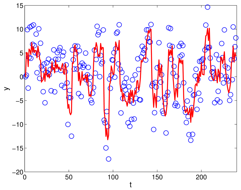
Figure 1: The noise free (solid line) and noisy outputs (circles).

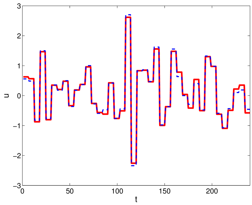
Figure 2: The estimated (dashed line) and the true input ${\bf u}$ (solid line).

To further study the robustness of BIL we carried out a Monte Carlo simulation. In the simulation, the noise level $\epsilon$ was varied between 0 and 5. For each noise level, 100 trials were carried out with different noise and input realizations. The true ARX model was kept fixed (the same as above). The results are summarized in Figure 3.

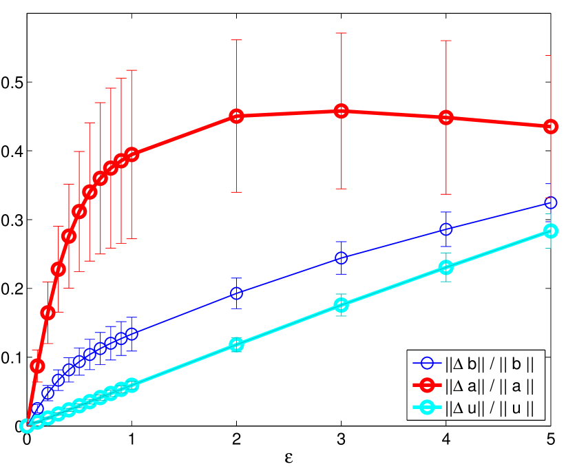
Figure 3: The relative errors along with their 0.5 standard deviation error bounds for varying noise levels.

The setup of above example does not give that ${\bf A}$ has full column rank. Nevertheless, a perfect result was obtained in the noise free case. It can however be verified that if ${\bf D}$ is instead generated by independently sampling each element from a unit Gaussian distribution (everything else unchanged), the resulting ${\bf A}$ has full column rank.

10 Conclusion

This paper presented a novel framework for blind system identification of ARX model. The framework uses the fact that the problem can be rewritten as a rank minimization problem. A convex relaxation is presented to approximate the sought ARX parameters and the unknown inputs.

References

- Abed-Meraim and Moulines (1994) K. Abed-Meraim and E. Moulines. A maximum likelihood solution to blind identification of multichannel FIR filters. In EUSIPCO, pages 1011–1015, 1994.
- Abed-Meraim et al. (1997) K. Abed-Meraim, Wanzhi Qiu, and Y. Hua. Blind system identification. Proceedings of the IEEE, 85(8):1310–1322, 1997.
- Abed-Meraim et al. (2006) K. Abed-Meraim, P. Loubaton, and E. Moulines. A subspace algorithm for certain blind identification problems. IEEE Transansactions on Information Theory, 43(2):499–511, September 2006.
- Ahmed et al. (2012) A. Ahmed, B. Recht, and J. Romberg. Blind deconvolution using convex programming. CoRR, abs/1211.5608, 2012.
- Bai and Fu (2002) E.-W. Bai and Minyue Fu. A blind approach to Hammerstein model identification. IEEE Transactions on Signal Processing, 50(7):1610–1619, 2002.
- Bai et al. (2010) E.-W. Bai, Q. Li, and S. Dasgupta. Blind identifiability of IIR systems. Automatica, 38(1):181–184, 2010.
- Bertsekas and Tsitsiklis (1997) D. P. Bertsekas and J. N. Tsitsiklis. Parallel and Distributed Computation: Numerical Methods. Athena Scientific, 1997.
- Bertsekas et al. (2003) D. P. Bertsekas, A. Nedic, and A. E. Ozdaglar. Convex Analysis and Optimization. Athena Scientific, 2003.
- Boyd et al. (2011) S. Boyd, N. Parikh, E. Chu, B. Peleato, and J. Eckstein. Distributed optimization and statistical learning via the alternating direction method of multipliers. Foundations and Trends in Machine Learning, 2011.
- Fazel et al. (2001) M. Fazel, H. Hindi, and S. P. Boyd. A rank minimization heuristic with application to minimum order system approximation. In Proceedings of the 2001 American Control Conference, pages 4734–4739, 2001.
- Goemans and Williamson (1995) M. X. Goemans and D. P. Williamson. Improved approximation algorithms for maximum cut and satisfiability problems using semidefinite programming. J. ACM, 42(6):1115–1145, November 1995.
- Grant and Boyd (2008) M. Grant and S. Boyd. Graph implementations for nonsmooth convex programs. In V. D. Blondel, S. Boyd, and H. Kimura, editors, Recent Advances in Learning and Control, Lecture Notes in Control and Information Sciences, pages 95–110. Springer-Verlag, 2008. http://stanford.edu/~boyd/graph_dcp.html.
- Grant and Boyd (2010) M. Grant and S. Boyd. CVX: Matlab software for disciplined convex programming, version 1.21. http://cvxr.com/cvx, August 2010.
- Hua (2002) Y. Hua. Blind methods of system identification. Circuits, Systems and Signal Processing, 21(1):91–108, 2002. ISSN 0278-081X.
- Ljung (1999) L. Ljung. System Identification — Theory for the User. Prentice-Hall, Upper Saddle River, N.J., 2nd edition, 1999.
- Löfberg (2004) J. Löfberg. YALMIP: A toolbox for modeling and optimization in MATLAB. In Proceedings of the CACSD Conference, Taipei, Taiwan, 2004. URL http://control.ee.ethz.ch/~joloef/yalmip.php.
- Lovász and Schrijver (1991) L. Lovász and A. Schrijver. Cones of matrices and set-functions and 0-1 optimization. SIAM Journal on Optimization, 1:166–190, 1991.
- Nesterov (1998) Y. Nesterov. Semidefinite relaxation and nonconvex quadratic optimization. Optimization Methods & Software, 9:141–160, 1998.
- Ohlsson et al. (2013) H. Ohlsson, A. Y. Yang, R. Dong, M. Verhaegen, and S. S. Sastry. Quadratic basis pursuit. CoRR, abs/1301.7002, 2013.
- Recht et al. (2010) B. Recht, M. Fazel, and P. Parrilo. Guaranteed minimum-rank solutions of linear matrix equations via nuclear norm minimization. SIAM Review, 52(3):471–501, 2010.
- Sato (1975) Y. Sato. A method of self-recovering equalization for multilevel amplitude-modulation systems. IEEE Transactions on Communications, 23(6):679–682, 1975.
- Shor (1987) N.Z. Shor. Quadratic optimization problems. Soviet Journal of Computer and Systems Sciences, 25:1–11, 1987.
- Sun et al. (1999) L. Sun, W. Liu, and A. Sano. Identification of a dynamical system with input nonlinearity. IEE Proceedings – Control Theory and Applications, 146(1):41–51, 1999.
- Tong et al. (1991) L. Tong, G. Xu, and T. Kailath. A new approach to blind identification and equalization of multipath channels. In 1991 Conference Record of the Twenty-Fifth Asilomar Conference on Signals, Systems and Computers, volume 2, pages 856–860, 1991.
- Van Vaerenbergh et al. (2013) S. Van Vaerenbergh, J. Vía, and I. Santamaría. Blind identification of SIMO Wiener systems based on kernel canonical correlation analysis. IEEE Transactions on Signal Processing, 61(9):2219–2230, 2013.
- Wang et al. (2007) J. Wang, A. Sano, D. Shook, T. Chen, and B. Huang. A blind approach to closed-loop identification of Hammerstein systems. International Journal of Control, 80(2):302–313, 2007.
- Wang et al. (2009) J. Wang, A. Sano, T. Chen, and B. Huang. Identification of Hammerstein systems without explicit parameterisation of non-linearity. International Journal of Control, 82(5):937–952, 2009.
- Wang et al. (2010) J. Wang, A. Sano, T. Chen, and B. Huang. A blind approach to identification of Hammerstein systems. In F. Giri and E.-W. Bai, editors, Block-oriented Nonlinear System Identification, volume 404 of Lecture Notes in Control and Information Sciences, pages 293–312. Springer London, 2010.
- Watson (1992) G.A. Watson. Characterization of the subdifferential of some matrix norms. Linear Algebra and its Applications, 170(0):33–45, 1992. ISSN 0024-3795.
- Zerva et al. (1999) A. Zerva, A.P. Petropulu, and P.-Y. Bard. Blind deconvolution methodology for site-response evaluation exclusively from ground-surface seismic recordings. Soil Dynamics and Earthquake Engineering, 18(1):47–57, 1999.
- Zerva et al. (2000) A. Zerva, A.P. Petropulu, and P.-Y. Bard. Blind system identification. In Proceedings of the 8th ASCE Joint Specialty Conference on Probabilistic Mechanics and Structural Reliability, PMC2000, University of Notre Dame, Indiana, USA, 2000.