The MICE Grand Challenge Lightcone Simulation II:
Halo and Galaxy catalogues

Abstract

This is the second in a series of three papers in which we present an end-to-end simulation from the MICE collaboration, the MICE Grand Challenge (MICE-GC) run. The N-body contains about 70 billion dark-matter particles in a $(3\,h^{-1}\,{\rm Gpc})^{3}$ comoving volume spanning 5 orders of magnitude in dynamical range. Here we introduce the halo and galaxy catalogues built upon it, both in a wide ($5000\,{\rm deg}^{2}$) and deep ($z<1.4$) lightcone and in several comoving snapshots. Halos were resolved down to few $10^{11}\,h^{-1}\,{\rm M_{\odot}}$. This allowed us to model galaxies down to absolute magnitude M${}_{r}<-18.9$. We used a new hybrid Halo Occupation Distribution and Abundance Matching technique for galaxy assignment. The catalogue includes the Spectral Energy Distributions of all galaxies. We describe a variety of halo and galaxy clustering applications. We discuss how mass resolution effects can bias the large scale $2$-pt clustering amplitude of poorly resolved halos at the $\lesssim 5\%$ level, and their $3$-pt correlation function. We find a characteristic scale dependent bias of $\lesssim 6\%$ across the BAO feature for halos well above $M_{\star}\sim 10^{12}\,h^{-1}\,{\rm M_{\odot}}$ and for LRG like galaxies. For halos well below $M_{\star}$ the scale dependence at $100\,h^{-1}\,{\rm Mpc}$ is $\lesssim 2\%$. Lastly we discuss the validity of the large-scale Kaiser limit across redshift and departures from it towards nonlinear scales. We make the current version of the lightcone halo and galaxy catalogue (MICECATv1.0) publicly available through a dedicated web portal, http://cosmohub.pic.es, to help develop and exploit the new generation of astronomical surveys.

1 Introduction

Over the past two decades our understanding of the Universe has improved dramatically, in good part thanks to ground-breaking observational campaigns (Riess et al., 1998; Perlmutter et al., 1999; Bennett et al., 2003; Cole et al., 2005; Tegmark et al., 2004). Although very successful this effort has opened the window to yet larger challenges that remain unresolved. For instance deciphering the reason for the late time acceleration of the Universe, what can result in totally new forms of energy or in the need to re-formulate Einstein’s theory of gravity. There is also a need to shed light into the nature of dark-matter and the neutrino sector, and of a better understanding of the galaxy formation process.

The community has responded to these challenges with a multi-probe approach consisting of several observational tests carried on independently or combined. From cluster abundance and weak lensing studies to large scale galaxy clustering including the baryon acoustic oscillations and redshift space distortions (WiggleZ, BOSS, CFHTLenS, DES, Euclid, DESI) in addition to state-of-the-art supernovae and CMB experiments (Planck Collaboration et al., 2014; Astier et al., 2006) and deep surveys such as GAMMA or PAU, among many others.

Run			$N_{{\rm part}}$	$L_{{\rm box}}/\,h^{-1}\,{\rm Mpc}$	$PMGrid$	$m_{p}/(10^{10}\,h^{-1}\,{\rm M_{\odot}})$	$l_{{\rm soft}}/\,h^{-1}\,{\rm Kpc}$	$z_{{\rm i}}$	$Max.TimeStep$
MICE-GC			$4096^{3}$	$3072$	$4096$	$2.93$	$50$	$100$	$0.02$
MICE-IR			$2048^{3}$	$3072$	$2048$	$23.42$	$50$	$50$	$0.01$
MICE-SHV			$2048^{3}$	$7680$	$2048$	$366$	$50$	$150$	$0.03$

Table 1: Description of the MICE N-body simulations. $N_{{\rm part}}$ denotes number of particles, $L_{{\rm box}}$ is the box-size, $PMGrid$ gives the size of the Particle-Mesh grid used for the large-scale forces computed with FFTs, $m_{p}$ gives the particle mass, $l_{soft}$ is the softening length, and $z_{in}$ is the initial redshift of the simulation. All simulations had initial conditions generated using the Zeldovich Approximation. Max. Timestep is the initial global time-stepping used, which is of order $1\%$ of the Hubble time (i.e, $d\log a=0.01$, being $a$ the scale factor). The number of global timesteps to complete the runs were $N_{steps}\lower 2.15277pt\hbox{$\;\buildrel>\over{\sim}\;$}2000$ in all cases. Their cosmological parameters were kept constant throughout the runs (see text for details).

Mag Limit		N. of Galaxies	Sat. Fraction	$\langle M^{all}_{h}\rangle$	$\langle M^{cen}_{h}\rangle$	$M^{cen}_{h,\rm min}$	Red Cen. [%]	Red Sat. [%]
$M_{r}<-19$		$1.92\times 10^{8}$	$0.23$	$1.0\times 10^{12}$	$6.35\times 10^{11}$	$2.23\times 10^{11}$	$35$	$77$
$M_{r}<-20$		$8.01\times 10^{7}$	$0.25$	$2.38\times 10^{12}$	$1.57\times 10^{12}$	$6.04\times 10^{11}$	$46$	$80$
$M_{r}<-21$		$1.42\times 10^{7}$	$0.24$	$8.29\times 10^{12}$	$6.74\times 10^{12}$	$1.94\times 10^{12}$	$62$	$87$
$M_{r}<-22$		$2.3\times 10^{5}$	$0.13$	$5.62\times 10^{13}$	$5.5\times 10^{13}$	$7.94\times 10^{12}$	$85$	$98$

Table 2: Some basic properties of the MICE lightcone galaxy catalogue that we make publicly available with this series of papers. The catalogue subtends one octant of the full sky and reaches $z=1.4$ with no simulation box repetition. It is absolute magnitude limited in the r-band, $M_{r}>-18.9$ (corresponding to $M_{h}>2\times 10^{11}\,h^{-1}\,{\rm M_{\odot}}$). The table lists the number of galaxies, satellite fraction, and mean host halo mass for all galaxies (“central+satellites”) and “centrals only” above some magnitude limits. Also listed is the minimum host halo mass for centrals and the fraction of red centrals and red satellites (w.r.t. all centrals and all satellites above the given $M_{r}$ cut).

The task ahead is nonetheless very hard because these datasets will have an unprecedented level of precision, and thus require ourselves to match it with well suited analysis tools. In this regard, large and complex simulations are becoming a fundamental ingredient to develop the science and to properly interpret the results (e.g. see Fig. 2 in Fosalba et al. (2013)).

This paper is the second in a series of three in which we present a state-of-the-art end-to-end simulation composed of several steps, with a strong focus in matching observational constrains and a galaxy catalogue in the lightcone as an end-product. This was built upon a new N-body simulation developed by the MICE collaboration, the MICE Grand Challenge run (MICE-GC), that includes about 70 billion dark-matter particles in a box of about $3\,h^{-1}\,{\rm Gpc}$ aside. Details of the N-body run are given in Table 1 and in the companion Paper I (Fosalba et al., 2013). The N-body set up was a compromise between sampling the largest volume possible without repetition, e.g. the one of the ongoing DES survey (The Dark Energy Survey Collaboration, 2005), while maintaining a high mass resolution, of $\sim 10^{10}\,h^{-1}\,{\rm M_{\odot}}$ (necessary to reach the observed magnitude limits of current and some future observations). The MICE-GC N-body run is introduced in Paper I, with an elaborated discussion of the resulting dark-matter clustering properties and the comparison with lower resolution runs.

Next we built halo and galaxy catalogues both in comoving and lightcone outputs. By construction the galaxy catalogue matches observed luminosity functions, color distributions and clustering as a function of luminosity and color at low-$z$ (Blanton et al., 2003; Blanton et al., 2005; Zehavi et al., 2011). Galaxy properties are then evolved into the past-lightcone using evolutionary models. Some properties of the resulting lightcone galaxy catalogue are given in Table 2. Note that we also built galaxy catalogues for the comoving outputs, which are very useful for some concrete studies. The discussion of the halo and galaxy catalogue construction, their properties and their potential in terms of clustering studies are the subject of this paper (Paper II).

Lastly we used the dark-matter distribution in the lightcone discussed in Paper I to build all sky lensing potentials and hence add lensing properties to the galaxies such as shear and kappa values, magnified luminosities and positions, and ongoing work with intrinsic alignments. The details of this procedure, its validation and applications are the subject of the companion Paper III (Fosalba et al., 2015).

We make the first version of the MICE-GC lightcone galaxy and halo catalogue (MICECAT v1.0) publicly available at the dedicated web portal http://cosmohub.pic.es, with the hope that can be of value to help develop the science, the design and the exploitation of new wide-area cosmological surveys.

In this paper, besides the catalogue validation, we study three concrete issues: (1) how the halo clustering on large-scales depends on the mass resolution of the underlying N-body simulation for fixed halo mass samples (2) the halo and galaxy clustering from small scales to very large ones with a focus on scale dependent bias and cross-correlation coefficients (3) limitations of the Kaiser limit in Redshift Space and in particular the impact of satellite galaxies in the multipole moments of the anisotropic clustering.

This paper is organized as follows: Section 2 presents the MICE-GC catalogue of friend-of-friends halos, the mass function determined from the comoving and lightcone outputs, as well as some clustering properties. Section 3 describes the galaxy mocks built upon the MICE-GC halos and their properties. In particular, we show predictions from the galaxy mock for the clustering and color distribution compared to observations at high-$z$ where these properties were not matched by construction. In Sec. 4 we discuss mass resolution effects in 2 and 3 point halo clustering statistics. In Sec. 5 we investigate the scale dependence of bias for several halo and galaxy samples. In Sec. 6 we turn into redshift space and study the applicability of the large-scale Kaiser limit in the lightcone, and the generation of non-trivial multipole moments due to satellite motions within halos. Finally, Sec. 7 describes our public catalogue release and Sec. 8 summarizes our main results and conclusions.

2 Halo Catalogues

One of the fundamental data products of the MICE-GC simulation are halo catalogues, which we have built out of both, comoving and lightcone dark-matter outputs subtending the full sky.

We identified halos using a Friend-of-Friend (FOF) algorithm with a standard linking length of 0.2 (in units of the mean inter-particle distance) both for the comoving outputs and the lightcone (as the mean matter density is independent of redshift). We used a FoF code built upon the one publicly available at www-hpcc.astro.washington.edu, with some concrete improvements needed to handle large amount of data in due time (each MICE-GC output is about 1TB of data).

The resulting halo catalogues contain basic halo information as well as positions and velocities of all the particles forming each halo. This allowed us to measure also halo 3D shapes and angular momentum. This is a key ingredient for a number of further applications, but in particular it will permit to incorporate intrinsic alignments in the lensing catalogues discussed in the companion Paper III.

In what follows we validate the abundance and clustering of the MICE-GC halo catalogues. In Sec. 4 we go one step further and compare the clustering results with those of previous runs to investigate mass resolution effects in halo bias.

2.1 Mass function

Figure 1: Mass Function in MICE at $z=0$. Black symbols show the halo abundance in the Grand Challenge run while red symbols correspond to the intermediate simulation with the same cosmology but 8 times worse mass resolution ($m_{p}=2.9\times 10^{10}\,h^{-1}\,{\rm M_{\odot}}$ vs. $m_{p}=2.3\times 10^{11}\,h^{-1}\,{\rm M_{\odot}}$). The dashed line results from a fit to a series of MICE simulations (Crocce et al. 2010). Abundances are depicted relative to the Sheth and Tormen model and error-bars were estimated using jack-knife resampling.

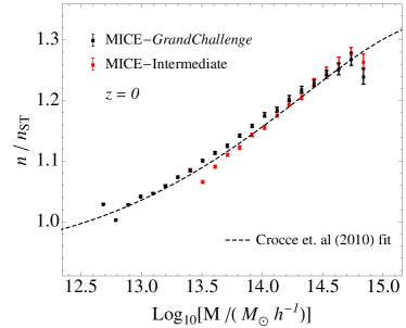
Let us begin by looking at the halo abundance. The halo finder in MICE-GC yields about 172 million FoF halos with 20 or more particles in the comoving output at $z=0$, and about 74 millions in each octant of the full sky lightcone up to $z=1.4$ (these numbers rise to 350 million and 157 millions respectively if we instead consider 10 or more particles, as we do in Sec. 3). Figure 1 shows the measured halo mass function at $z=0$ in MICE-GC compared to both the one measured in MICE-IR and the numerical fit to a large set of MICE simulations from Crocce et al. (2010) (we depict the ratio to the well known Sheth & Tormen (1999) mass function to highlight details). For each simulation, we only show a mass-range in which halos are well sampled containing $\sim 150$ or more particles. At the high-mass end, were halos are very well sampled in both MICE-GC and MICE-IR, both mass functions agree very well. Towards the regime of $M/(\,h^{-1}\,{\rm M_{\odot}})\sim 10^{13.5}$ to $10^{14}$ MICE-GC has a slightly larger halo abundance, by $\sim 2\%$ (a trend that continues to lower mass, not shown in Fig. 1). Within $2\%$ the fit from Crocce et al. (2010) reproduces the shape of the MICE-GC mass function.

We note that in defining our halo masses we have accounted for the Warren correction for discrete halo sampling, unless otherwise stated (Warren et al. (2006); Crocce et al. (2010); Bhattacharya et al. (2011) and ref. therein). This means that $M_{h}=n_{h}m_{p}(1-n_{h}^{-0.6})$, with $m_{p}$ being the particle mass and $n_{h}$ the corresponding number of particles in halo. This brings the shape of both mass functions into a much better agreement across the mass range shown in Fig. 1. In addition MICE-IR have been corrected for transients as described in Crocce et al. (2010) (this correction is negligible for $M/(\,h^{-1}\,{\rm M_{\odot}})\sim 10^{13.5}$ and $\sim 5\%$ by $M/(\,h^{-1}\,{\rm M_{\odot}})\sim 10^{15}$). Lastly we have also accounted for the fact that the initial transfer function in MICE-IR was EH instead of CAMB, see Fig. 5 in Paper I (this introduces a $\lesssim 1\%$ correction, depending on halo mass).

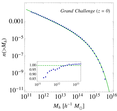
Later we will argue that one possible way of reaching fainter magnitudes when building galaxy mock catalogues is by using poorly resolved structures (halos of $\gtrsim 10$ particles). It is then interesting to investigate the abundance of these objects. Figure 2 shows the cumulative mass function measured in MICE-GC down to 10 particle halos ($M_{h}=2.2\times 10^{11}\,h^{-1}\,{\rm M_{\odot}}$) compared to the model prediction using the Crocce et al. (2010) fit . The cumulative abundance is $10\%-15\%$ lower than the prediction at this limit, but it goes to within $5\%$ for halos with $\sim$ 40 particles already.

Figure 2: Cumulative mass function measured in MICE-GC down to the extreme regime of poorly resolved halos with 10 or more particles. The inset panel show the ratio to the prediction for this quantity using the fit from Crocce et al. (2010), which is depicted by a solid green line in the main panel.

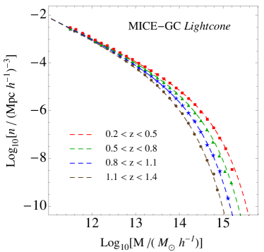
In turn the redshift evolution of the MICE-GC halo abundance is shown in Fig. 3, with the halo mass function measured in the lightcone for several consecutive redshifts bins, as detailed in the inset labels. The evolution is in good agreement with the fit from Crocce et al. (2010), which does not assume universality. Notice how $M_{\star}$ (roughly the mass beyond which the abundance is exponentially suppressed) decreases with redshift, as expected in hierarchical clustering (e.g. Cooray & Sheth (2002)).

Figure 3: Halo abundance as a function of redshift in the MICE-GC lightcone for several consecutive redshift bins. The theory model shown, from Crocce et al. 2010, does not assume universality.

2.2 Halo Clustering at large scales

2.2.1 Power Spectrum: Clustering amplitude at $z=0$

We now discuss some basic characterization and validation of the halo clustering in the comoving snapshot at $z=0$, with a more in depth analysis postponed to Secs. 5 and 6.

Figure 4: Large-scale halo and galaxy (auto) power spectrum in the MICE-GC comoving output at $z=0$ (over a smooth broad-band power, without shot-noise correction). We display three self corresponding magnitude and mass threshold samples. For a given halo mass threshold we select the corresponding magnitude limited galaxy sample from the mean “halo mass - central galaxy luminosity” relation. We then consider both “centrals only” or “central+satellites” in each sample. The dashed black line corresponds to the clustering of dark matter. The figure shows that the large volume and good mass-resolution in MICE-GC allows to study large-scale clustering from anti-biased or un-biased samples to highly biased ones, with percent level error-bars at BAO scales. In addition notice how in general satellite galaxies increase the clustering amplitude above the “centrals only” without introducing noticeable extra scale-dependence.

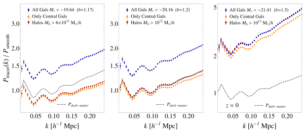
The combination of large volume and good mass resolution of MICE-GC allows to study with high precision a range of quite different halo samples in terms of clustering, from anti-biased and un-biased to highly biased ones. The red symbols in Fig. 4 show the $z=0$ halo-halo power spectrum for 3 such samples in MICE-GC ($b_{h}=0.95,1$ and $1.5$ in left, middle and right panel respectively), and how precise they trace the BAO feature. The black dashed line corresponds to the measured dark-matter clustering, which on these scales agrees with perturbation theory predictions (RPT, Crocce & Scoccimarro (2008)) and numerical fits (Takahashi et al., 2012; Heitmann et al., 2014) to $2\%$ or better, see Paper I. All measured spectra in Fig. 4 have been divided by a smooth broad-band power to highlight narrow band features, and are not corrected by shot-noise. Reported error bars assume the FKP approximation (Feldman et al., 1994): $\sigma_{P_{k}}=\sqrt{N_{m}(k)/2}(P_{k}+1/\bar{n})$, where $N_{m}$ is the number of Fourier modes used to measure the band-power $P_{k}$ and ${\bar{n}}$ the tracer comoving number density.

One basic validation is the comparison of the bias measured from $P_{hh}/P_{mm}$ to the prediction using the peak background split argument (PBS) (Bardeen et al., 1986; Cole & Kaiser, 1989), employing the mass function fit to MICE runs from Crocce et al. (2010) as input to the PBS formulas (following Eq. (23) in Manera et al. (2010)). For the samples in Fig. 4 we find,

$${\rm Halo\,Sample\ \ \ \ \ \ \ } {\rm b_{measured}} {\rm bias_{PBS}}$$

$$\ \ \ \ M_{h}/(\,h^{-1}\,{\rm M_{\odot}})>6\times 10^{11} 0.948\pm 0.002 \ \ 0.93$$

$$M_{h}/(\,h^{-1}\,{\rm M_{\odot}})>10^{12} 1.002\pm 0.002 \ \ 0.98$$

$$M_{h}/(\,h^{-1}\,{\rm M_{\odot}})>10^{13} 1.546\pm 0.009 \ \ 1.4$$

Figure 5: Symbols show the 2-point correlation function $\xi(r)$ (scaled by $r^{2}$) in FoF halos (with 20-50 particles) for three redshift bins in the lightcone (in real space). Dashed lines are the corresponding DM smoothed linear theory predictions (which resemble non-linear predictions). Notice how halo biasing for constant mass is roughly degenerate with growth, yielding a constant clustering amplitude.

The reported measured bias and errors were obtained from combining $P_{hh}$ and $P_{mm}$ into Eqs. (16) and (17) of Smith et al. (2007) for the first $10$ $k$-bins at the largest scales ($0.05<k/\,h\,{\rm Mpc}^{-1}<0.06$). The PBS prediction agree at the $10\%$ level for the most massive sample, in agreement with previous studies (Manera et al., 2010; Tinker et al., 2010). For $b\sim 1$ samples the matching improves to $\sim 2\%$. To our knowledge the performance of PBS in this low biasing regime has not been explored before.

2.2.2 Correlation Function: Halo Bias in the lightcone

We next explore how the clustering evolves with redshift using the lightcone halo catalogue (see also Sec. 6.1).

Figure 5 shows the effect of halo bias on the 2-point correlation at BAO scales, for a sample of FoF halos with masses $6\times 10^{11}<M_{h}/(\,h^{-1}\,{\rm M_{\odot}})<1.5\times 10^{12}$ (more than 20 particles and less than 50 particles). We can see how the main effect of halo biasing with redshift (for constant halo mass) is to change the amplitude of the correlations in a way that is roughly degenerate with the linear growth in the dark-matter (DM) distribution. The linear bias $b_{1}$, defined as the square root of the ratio of the halo correlation to the corresponding DM correlation is about $b\simeq 0.9$ for the lower redshift and $b\simeq 1.5$ for the largest one. These values result in halo clustering amplitudes that are quite similar at different redshifts (i.e. $b\propto 1/D(z)$), in contrast to the corresponding DM results shown in solid lines. Note that the BAO peak can be well detected despite the bias. We leave for Sec. 5 a more detailed study of scale dependent bias across the BAO scales.

Lastly we note that the binning used in Fig. 5 (and later in Fig. 12) is rather broad to make the figure less crowded and reduce the covariance between data-points, but we have checked that a narrower binning does not change the results.

3 Galaxy Catalog

3.1 Catalog construction and basic properties

We have built galaxy mock catalogues from both lightcone and comoving outputs, starting from the corresponding halo catalogues discussed in the previous section. These mocks are generated to provide a tool to design, understand and analyze cosmological surveys such as PAU, DES and Euclid.

We have used a new hybrid technique that combines halo occupation distribution (HOD; e.g. Jing et al. (1998); Scoccimarro et al. (2001); Berlind & Weinberg (2002)) and halo abundance matching (HAM; e.g. Vale & Ostriker (2004); Tasitsiomi et al. (2004); Conroy et al. (2006)) prescriptions. We do not intend to reproduce the details of the catalogue generation here, but just to present some validation results to give an idea of how the mocks compare to observations and therefore provide a glimpse of their possible use. The galaxy assignment method is described in full detail in Carretero et al. (2015). Further details regarding redshift evolution of galaxy properties will be given in Castander et al. (2014), in preparation.

We stress however that our galaxy catalogue is not intended to reproduce one given galaxy population, as typically needed for spectroscopic surveys (e.g. the CMASS sample for BOSS in Manera et al. (2013) and White et al. (2014)). In that sense our scope is larger and more complex as we aim to reproduce the abundance and clustering across luminosity and color space, and its evolution with redshift (i.e. luminosity functions, color-magnitude diagrams, clustering as a function of color and magnitude cuts, and more).

In order to generate the galaxy catalogue, we assume that halos are populated by central and satellite galaxies. We assume that all halos have one central galaxy and a number of satellites given by an HOD prescription, which determines the mean number of satellite galaxies as a function of the halo mass. We assign luminosities to the central galaxies with a halo mass-luminosity relation computed with HAM techniques, matching the abundances of the galaxy luminosity function and the halo mass function. We need to introduce scatter in this relation in order to fit the galaxy clustering at bright luminosities. We then populate the halos with the number of satellites given by the HOD parameters that fit the resulting 2-point projected correlation function of galaxies to observations. We assign luminosities to the satellites to preserve the observed galaxy luminosity function and the dependence of clustering with luminosity, imposing the additional constraint that the luminosity of satellites in a given halo cannot exceed the luminosity of the central galaxy by more than 5% (Carretero et al., 2015).

Central galaxies are placed at the halo center of mass. Satellite galaxies are positioned into the halos following a triaxial NFW profile with fixed axis ratios (e.g. Jing & Suto (2002)). In order to fit clustering observations as a function of luminosity on small scales (one-halo regime) we need to concentrate satellite galaxies more than the standard dark-matter distribution relation given in Bullock et al. (2001). Hence we employ a concentration parameter in each axis given by the relation in Bullock et al. (2001) with slight changes depending on galaxy luminosities (Carretero et al., 2015). Similar conclusions are found in Watson et al. (2012).

Central galaxies are assigned the center of mass velocity of the host halo. In turn, we assume that satellite galaxies have in addition a virial motion on top of the bulk halo velocity (Sheth & Diaferio, 2001). We assume that the halos are virialized and that the satellites velocities within the halo have a velocity dispersion given by the halo mass (Bryan & Norman, 1998). We assign velocities to the satellite galaxies drawing each component of the velocity vector from three independent Gaussian distribution of dispersion $1/\sqrt{3}$ of the global velocity dispersion of the halo. We discuss the impact of this assumption on anisotropic clustering measurements in Sec. 6.3.

Figure 6: Scatter plot of apparent magnitudes, $i_{AB}$, versus redshifts for a random set of galaxies in our mock catalog. There are missing faint galaxies at low redshift because the sample is limited in absolute magnitude. At $z\simeq 1$ the catalog is complete to $i_{AB}\sim 24$, while at $z\simeq 0.5$ is complete only to $i_{AB}\sim 22$.

Lastly we assign spectral energy distributions to the galaxies with a recipe that preserves the observed color-magnitude diagram and the clustering as a function of color.

The method has been tuned to match observational constraints from SDSS at low redshift where they are more stringent (detailed further below). We nevertheless apply the same method throughout the lightcone at all redshifts with slight modifications. In order to reproduce the observed galaxy properties at higher redshifts, we impose evolutionary corrections to the galaxy colors and obtain a final spectral energy distribution (SED) resampling from the COSMOS catalogue of Ilbert et al. (2009) galaxies with compatible luminosity and (g-r) color at the given redshift. Once each galaxy has a SED assigned, we can compute any desired magnitude to compare to observations.

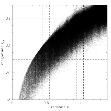
One feature of the current version of the galaxy mock catalogue presented in this paper is that it is absolute magnitude limited. This is inherited from the fact that is generated from a parent halo catalogue that is mass limited. Current cosmological imaging surveys are normally apparent magnitude limited down to faint magnitudes. The version of the catalogue that is now made public is complete down to $i<24$ for redshifts $z\gtrsim 0.9$. For lower redshifts the catalog is complete only to brighter magnitudes as illustrated by Fig. 6.

In order to overcome this incompleteness at low z we have started populating sub-resolved halos (thanks to the fact that at the resolution limit of MICE-GC the halo bias has a weak dependence with mass) yielding catalogues which are complete to observed magnitudes $i\sim 24$ (for all $z<1.4$). This additional work, more focused on modeling faint galaxy populations at low redshift, will be presented in a follow up paper.

Figure 7: Contour plots for the (g-r) vs. (r-i) color distribution in the COSMOS sample (red) and the MICE galaxy mock (blue), for galaxies at z$<$0.8 (top panel) and between 0.8$<$z$<$1.4 (bottom panel). Notice that these distributions are not matched by construction in our mock but rather are the result of stellar evolution models used to populate halos in the past lightcone.

By construction our catalogue reproduces the local observational constraints provided by the Sloan Digital Sky Survey (SDSS, York et al. (2000)). We reproduce the local luminosity function (Blanton et al., 2003) and color distributions (Blanton et al., 2003; Blanton et al., 2005). The method has also been adjusted to match the clustering as a function of luminosity and color following observational constraints from the SDSS (Zehavi et al., 2011). Hence, we now present a comparison of the photometric and clustering properties of the galaxy catalogue to observations at higher redshift where the method has not been tuned.

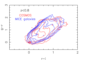
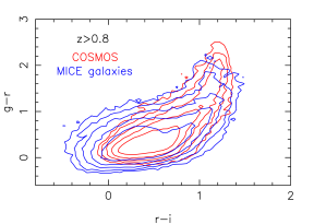
As an example of such comparison, Fig. 7 shows the contour plots of the (g-r) vs. (r-i) color distribution of the COSMOS catalogue of Ilbert et al. (2009) and our mock catalogue. The COSMOS data has been cut in absolute magnitude, $M_{V}<-19.0$, and redshift, $z<1.4$, to expand the same ranges as the MICE catalogue. On the top panel we present the galaxies at $z<0.8$, where the overall color-color distribution of our mock is a reasonable fit to observations. On the bottom panel we show the distribution of galaxies at $0.8<z<1.4$. In this case our catalogue is also an acceptable fit to observations albeit slightly over-producing blue galaxies.

Figure 8: Angular two point correlation function of the COSMOS (black dots and error bars) and MICE-GC catalogues (red solid line) at redshift $z=1.0$ for a magnitude limited sample $17<i_{AB}<24$. We also plot the MICE dark matter angular correlation function (blue dashed line) for comparison. In this plot, the MICE correlation has been computed in an area sixty times that of the COSMOS catalogue using the same mask. Given the larger area of the MICE catalogue and to avoid overcrowding the plot, we do not show the MICE error bars.

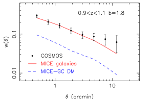
Turning to clustering properties, in Fig. 8 we compare the two point angular correlation function of the COSMOS catalogue (black dots and error bars) to our mock catalogue (red solid line) at redshift $z=1.0$. In both catalogues, we have selected all galaxies in the redshift range $0.9<z<1.1$ and galaxy magnitude $17.0<i<24$. The value of the correlation amplitude is very similar, except at scales larger than 5 arc-minutes, where the COSMOS amplitude is larger than the catalogue (although at the 1-$\sigma$ level). The COSMOS field presents an overdensity at $z\sim 0.9$ in its redshift distribution and is observed to have somewhat larger clustering amplitude than other fields (Skibba et al., 2014). For comparison we also calculate the dark matter two point angular correlation function (blue dashed line), from which one can infer the bias of the sample to be $b\sim 1.8$ at these scales.

Figure 9: Top Panel: Angular two point correlation function of the COSMOS (circles with jack-knife errorbars) at photometric redshift $0.45<z<75$ and for a galaxy sample with $17.5<i_{AB}<22.5$. Triangles with errorbars correspond to the mean and dispersion of 50 COSMOS like MICE-GC catalogues. We use the same magnitude and photo-z limits for MICE as in COSMOS. The redshift distribution of galaxies is shown in the inset for both COSMOS (continuous) and MICE (dashed), with $\langle z\rangle=0.61$. We also plot the DM prediction for MICE as different lines, as indicated in the top label. Bottom Panel: Measured galaxy bias for COSMOS (circles) and MICE (triangles).

In the top panel of Fig. 9 we show the corresponding results for a redshift slice of $0.45<z<75$. Here we restrict both samples to brighter galaxies $17.5<i_{AB}<22.5$, so that both are complete (see Fig. 6). The COSMOS photo-z errors are also much smaller for these brighter galaxies, so the comparison is more direct. We also include the DM linear prediction (dotted), the non-linear DM prediction (continuous) and the prediction including the finite area correction (dashed line) resulting from the integral constrain in the COSMOS area (of about $1.4\,{\rm deg}^{2}$). We have simulated the COSMOS sample with 50 separate MICE-GC regions of equal size, same magnitude limit ($17.5<i<22.5$) and same redshifts distribution (shown in the inset). The COSMOS data and the MICE-GC catalog agree remarkably well. In the bottom panel we also show the effective galaxy bias $b$ estimated as $b(\theta)=\sqrt{w_{GAL}(\theta)/w_{DM}(\theta)}$, the ratio of the galaxy to non-linear DM prediction. The results are quite consistent between MICE-GC and COSMOS, despite the fact that MICE galaxy catalog was not built to match clustering by construction at these redshifts.

As a further validation we have compared the clustering in our catalogue to the one in the CMASS sample of the SDSS-III BOSS survey, on BAO scales. Note that this test is quite more challenging than before as it involves both a magnitude and a color selection of galaxies evolved in the past light-cone. We built a MICE-CMASS sample by applying the same selection for luminous red galaxies described in Eqs.(1-6) in Anderson et al. (2012). In the current version of the MICE-GC catalogue there is no evolution of the luminosity function beyond the one of the underlying mass function. Before doing a combined color and luminosity cut is important to account for this evolution . Hence we first correct the absolute magnitudes according to a functional fit derived by abundance matching between the evolving galaxy luminosity function and the halo mass function, which was not included in the MICECAT v1.0 release, $M_{r}^{evolved}=M_{r}+0.92*(atan(1.5*z)-0.149)$, and then impose the criteria $17.5<i<19.9$. Next we impose the color selection $d_{\perp}>0.46$ and $i<20.13+1.6(d_{\perp}-0.8$ where $d_{\perp}=r-i-(g-r)/8.0)$. Note that these values are slightly different than the ones used in CMASS (Anderson et al. (2012)). This is due to our galaxies being slightly bluer in this region of color space. The resulting catalogue has about the same number of galaxies ($\sim 445000$, if normalized to the $5000\,{\rm deg^{2}}$ of MICE-GC) and a very similar redshift distribution as the BOSS-CMASS, starting at $z\sim 0.4$ and falling off by $z\sim 0.7$. This is shown in Fig. 10. We then apply the redshift selection $0.43<z<0.7$, as done in Anderson et al. (2012).

Figure 10: A MICE-GC luminous red galaxy (LRG) sample. Solid black line (labeled MICE-CMASS) is the redshift distribution for an LRG sample in the MICE-GC catalogue following the color and magnitude selection criteria as the SDSS-III BOSS CMASS sample in Anderson et al. (2012). Filled dots is the actual distribution from CMASS-DR10. After the color selection the redshift distribution of MICE-CMASS matches very well CMASS-DR10. Dashed line corresponds to a sample selected only in absolute luminosity such as to yield the same clustering as DR10 (see Fig. 11) and the same total number of objects.

Figure 11: Quadrupole and Monopole correlation functions for the CMASS samples built from the MICE-GC lightcone catalogue, see Fig. 10. MICE-CMASS is shown in solid black while the actual CMASS DR10 measurements with filled symbols. The overall shape and BAO position is well traced by MICE-CMASS, while the bias is $\sim 10\%$ higher (see text for details). Dashed line corresponds to a $M_{r}<-21.2$ sample in MICE-GC, that compares better at the clustering level.

We next measured the monopole and quadrupole correlation functions, focusing on large BAO scales. This is shown in Fig. 11 that compares our clustering estimate in the BOSS CMASS-DR10 sample with the one over the CMASS selection of MICE galaxies. Both the shape and BAO scale are quite well reproduced by our catalogue. While the relative linear bias of MICE-CMASS is $\sim 10\%$ higher than the one in CMASS-DR10, both in monopole and quadrupole. There are several factors that can contribute to this small discrepancy. First, the MICE cosmology is different from the one in BOSS. Second, we have fixed HOD parameters to clustering at $z\sim 0$, so we do not expect a perfect match at higher redshift. This probably needs some HOD evolution other than the evolution in halo properties (for example in the mass-luminosity scatter which we apply always after the same luminosity threshold across redshift). Third, MICE-CMASS has $27\%$ satellites which is a factor of 3 times larger than BOSS predictions (Tojeiro et al., 2012). As we fixed the total galaxy abundance, a lower satellite fraction requires including more central galaxies, which by construction have smaller halo mass and therefore smaller bias. The mean halo mass in MICE-CMASS is $M_{h}=3.3\times 10^{13}\,h^{-1}\,{\rm M_{\odot}}$ which is a factor $2$ times higher than that expected in BOSS-CMASS. Such increase of a factor of 2 in halo mass can yield a $\sim 10\%$ increase in halo bias, in agreement with our findings. An alternative sample can be based on a simple absolute luminosity selection tuned such as to match the CMASS clustering rather than the redshift distribution. We found that we needed to cut MICE-GC to $M_{r}<-21.2$, which turns out very close to the actual minimum luminosity of BOSS-CMASS galaxies. After the luminosity selection we dilute MICE-GC to have the same number of objects as BOSS-CMASS. The redshift distribution is shown by a dashed line in Fig. 10, while the clustering in Fig. 11. The later agrees very well with CMASS-DR10 although there is no color selection imposed.

Although we have shown some concrete examples, the overall comparison between photometric and clustering properties of our catalogue to observations is good. This validates our approach in constructing the galaxy mock catalogue where we have applied stellar evolutionary corrections to the colors of the galaxies to construct the mock catalogue in the lightcone extrapolating the other low redshift recipes to higher redshifts. We have also discussed a simple implementation for evolution in galaxy luminosity, particularly relevant for narrow magnitude range selections.

3.2 Galaxy Clustering vs. Halo Clustering

The HOD prescription described above and used to populate the MICE-GC simulation with galaxies is based on matching the observed luminosity function and the small scale galaxy clustering ($r\lesssim 30\,h^{-1}\,{\rm Mpc}$). In this section we investigate what it implies for the clustering of galaxies on large-scales, in particular how this compares to the halo clustering already discussed.

Figure 4 has three panels corresponding to the power spectrum of anti-biased, unbiased and highly biased halo samples discussed in Sec. 2.2.1. In each panel we now include the clustering of galaxies brighter than the luminosity set by the corresponding mass-luminosity relation from the HOD+HAM prescription. We divide the (magnitude limited) galaxy sample into centrals only (orange symbols) and central+satellites (blue symbols). The left-most panel shows that faint central galaxies have almost the same clustering as their host halos. This is because the mass-luminosity relation at this regime is one-to-one (and the clustering is dominated by the most abundant galaxies). The addition of satellites boost the clustering signal because faint satellites can live in massive halos. On the other end bright central galaxies (right most panel) have less clustering strength than their corresponding halos from the mean halo mass - central luminosity relation. This is due to the scatter in $L_{cen}=L(M_{h})$, for fixed mass. Hence, a sample of centrals with $L>L_{\star}=L(M_{\star})$ has galaxies residing in halos with $M<M_{\star}$, what determines the (smaller) galaxy bias. Again adding the satellites boost the signal, in this particular case to match that of the halos (right panel of Fig. 4).

Figure 12: Galaxy 3D monopole correlation function in the lightcone (open circles) for three redshift bins and a magnitude limited sample $r<24$ (to compare with Fig. 5). Dashed lines are the corresponding linear theory predictions for dark-matter in real-space, while solid lines include linear bias and redshift space distortions. The modeling, where bias has been obtained from real space measurements, agrees well with the galaxy monopole. In this case the bias evolves stronger than the growth such that the galaxy clustering amplitude increases with $z$, contrary to the case of halos.

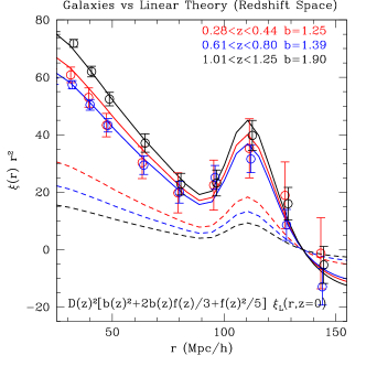
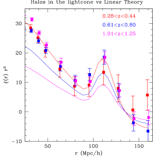
Lastly we turn to the evolution of clustering in the lightcone (see also Sec. 6.1). Figure 12 shows the monopole 3D correlation function measured at BAO scales in 3 redshift bins, for a magnitude limited galaxy sample ($r<24$) extracted from one octant of the MICE lightcone catalogue in redshift space. The dashed lines are the linear theory predictions for the corresponding dark-matter clustering in real-space at the given redshift. In turn the solid lines are the linear modeling for biasing and redshift space distortions (i.e. the Kaiser effect, Kaiser (1984), discussed in Sec. 6.1 in more detailed), angle averaged and evaluated at the mean of each redshift bin, see Eq. (10). The bias used in the modeling, and shown in the inset top-right labels, was obtained from the ratio of the two point correlation of galaxies to DM in real space. As we can see, the bias evolves quite strongly with redshift such that the clustering amplitude is largest for higher $z$ (where dark-matter clustering is weaker). This is because we have selected a magnitude limited sample, hosted by halos of increasing mass as we increase the redshift. This can be compared with Fig. 5 that has the corresponding study with halos of fixed mass showing a clustering amplitude that is roughly independent of redshift, meaning $b(z)\sim D(z)^{-1}$. Overall the linear modeling and the clustering measurements agree quite well on large scales in the lightcone provided with the larger statistical error bars (although more realistic from an observational point of view) compared to a comoving output, as we investigate in Sec. 5. The largest differences, still at the $1-\sigma$ level, are found at $0.28<z<0.44$ where sampling variance is largest and nonlinear effects strongest.

4 Resolution Effects in Halo Bias

Figure 13: Mass resolution effects in large-scale halo bias. Solid magenta lines correspond to the cross-correlation bias $b_{\rm X}=P_{hm}/P_{mm}$ measured in the MICE-GC run ($m_{p}=2.9\times 10^{10}\,h^{-1}\,{\rm M_{\odot}}$), while solid blue to the one measured in MICE-IR ($m_{p}=2.3\times 10^{11}\,h^{-1}\,{\rm M_{\odot}}$) at $z=0.5$. By default masses were corrected for finite halo sampling (Warren et al. 2006). The corresponding results for halo samples with the naive definition of mass $M_{h}=m_{p}n_{p}$ is depicted by the dashed lines in each panel.

In Paper I we studied how the matter distribution, in particular the clustering, depends on the simulation mass resolution. In this section we now extend that study to halo bias derived from both 2-pt and 3-pt clustering.

4.1 Results for 2-point correlations

Let us start with the 2-pt clustering in Fourier Space. In order to avoid noise due to low halo densities we look at the bias through the cross-correlation with the matter field, i.e.

$$b_{X}\equiv P_{hm}/P_{mm}$$ (1)

where $P_{hm}$ and $P_{mm}$ are the halo-matter and matter-matter power spectra respectively.

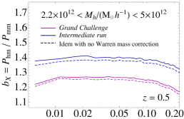
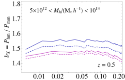
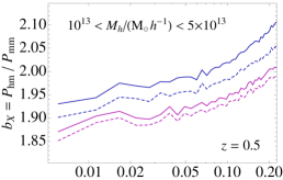
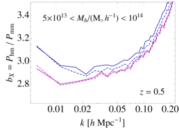
Figure 13 shows the large scale bias for different halo samples at $z=0.5$ selected by halo mass from simulations with different particle mass resolutions (MICE-GC and MICE-IR). We show $2.2\times 10^{12}<M_{h}/(\,h^{-1}\,{\rm M_{\odot}})<5\times 10^{12}$, $5\times 10^{12}<M_{h}/(\,h^{-1}\,{\rm M_{\odot}})<10^{13}$, $10^{13}<M_{h}/(\,h^{-1}\,{\rm M_{\odot}})<5\times 10^{13}$ and $M_{h}/(\,h^{-1}\,{\rm M_{\odot}})>10^{14}$, from top to bottom. In each panel MICE-GC measurements are depicted with solid magenta lines for samples in which halo masses have been corrected for finite sampling prior to selection (following the discussion in Sec  2.1), or with magenta dashed lines otherwise (here halo masses are defined simply as $m_{p}n_{p}$). Similarly for MICE-IR we use solid blue lines for “Warren” corrected masses, and dashed otherwise. In all cases the bias asymptotically approaches a scale independent value (although at progressively large scales with increasing halo mass, as expected) but with some slight differences depending on the simulation and halo mass range.

The top panel shows an extreme case of very poorly resolved halos (or “groups”), formed by 10 or more particles (up to 20). At this mass scale, MICE-GC halos have 80 to 170 particles. Even such extreme scenario yields quite reasonable clustering, with bias miss-estimated by $\sim 10\%$. Notice that we find higher clustering amplitude in the lower resolution simulation. We attribute this to the fact that poorly resolved halos are found preferentially closer of big halos and large structures in the low resolution run, that is in regions of high density. In turn low density regions are not as well resolved as in MICE-GC. This then biases up their clustering amplitude compared to the same mass halos in MICE-GC.

Doing the next step down in resolution, that is, comparing the clustering of $10$-particle halos in MICE-GC to theory predictions yield similar or even better results, with differences at the $5\%-10\%$ level (see Fig. 5 in Carretero et al. (2015)).

As pointed in the introduction, the next generation surveys will reach very faint magnitudes, challenging the resolution limit of current state-of-the-art simulations. Hence different approaches are being proposed to improve on mass resolution in approximated ways (Angulo et al., 2014). This panel intends to highlight one such approach which is simply to consider samples of very poorly resolved halos as long as one is interested in a halo mass scale $M_{h}<few\times 10^{12}\,h^{-1}\,{\rm M_{\odot}}$ where $b\lesssim 1$. At this scale halo bias becomes very weakly dependent on mass (e.g. Fig 5 in Carretero et al. (2015)). Thus for clustering measurements we can make a large error in the halo mass and still obtain accurate results. We should stress that we make this comment with the concrete goal of producing galaxy mock catalogues for data analysis. And is mainly relevant for completeness at low z because a galaxy catalog is typically limited in apparent magnitude therefore at high redshifts the galaxies are quite luminous and reside only in high mass halos. In turn error in the mass function (because of possible errors in halo mass) are automatically corrected by the calibration to low redshift galaxy luminosity with the SAM. The actual HOD parameters will be different than in a high resolution run, but the galaxy distribution will be quite similar. This is why we believe that halos with small number of particles can give results which are similar to those in higher resolution simulations

For the next mass bin in Fig. 13 MICE-IR halos have $\sim 20-50$ particles (as opposed to $170$ to $350$ in MICE-GC). The large-scale bias in MICE-IR is higher by $\sim 5\%$ if masses have been corrected or $3\%$ otherwise (see top panel in Fig. 13). The effect diminishes in the intermediate mass range at the middle panel (with $50$ to $200$ particles in MICE-IR halos) to $4\%$ and $2\%$ roughly. For well sampled halos ($M_{h}/(\,h^{-1}\,{\rm M_{\odot}})>5\times 10^{13}$, bottom panel) the bias recovered from MICE-IR is compatible within $\sim 1\%$ to the one from MICE-GC. For low number of particles per halo, the “Warren” correction seems to introduce a mass shift too large, that translates into artificial bias differences. A slight modification such as the one proposed in Bhattacharya et al. (2011) might alleviate this issue.

In summary the bias differences found between the different resolutions is within $3\%$ or better for well resolved halo masses, more standard in the literature, and up to $10\%$, for poorly resolved ones formed by as low as 10 particles. Similar conclusions were reached studying other redshifts. Hence this kind of effect can then be of importance for studies of accuracy in halo bias modeling, for instance the stated accuracy of peak-background split approach is $\lesssim 10\%$ (Manera et al., 2010; Tinker et al., 2010; Manera & Gaztañaga, 2011), not far from the effects purely dependent on simulation parameters discussed above.

4.2 Results for 3-points correlations

A further quantity of interest on top of the linear large-scale bias discussed above is the second order bias $b_{2}$ that naturally appears at the leading order in higher order correlations (Fry & Gaztanaga, 1993).

On large enough scales, where the fluctuations in the density field are smoothed so that the matter density contrast is of order unity or smaller, one can assume a general non-linear (but local and deterministic) relation between the density contrast in the distribution of halos $\delta_{h}$ and dark matter $\delta_{m}$ that can be expanded in a Taylor series

$$\delta_{h}=\sum_{k=0}^{\infty}\frac{b_{k}}{k!}\delta^{k}_{m}=b_{0}+b_{1}\delta_{m}+\frac{b_{2}}{2}\delta^{2}_{m}+\cdots,$$ (2)

where the $k=0$ term comes from the requirement that $<\delta_{h}>=0$. Within this local bias model, at scales where $\xi(r)\equiv\langle\delta_{m}^{2}(r)\rangle<1$, we can write the biased (halo or galaxy) two and three point functions to the leading order in $\xi$ (Fry & Gaztanaga, 1993; Frieman & Gaztanaga, 1994)

$$\xi^{h}(r) \simeq ~{}b_{1}^{2}~{}\xi(r)$$

$$\zeta^{h}(r_{12},r_{23},r_{13}) \simeq b_{1}^{3}\zeta(r_{12},r_{23},r_{13})+$$ (3)

$$+\,b_{1}^{2}b_{2}\left(\xi(r_{12})\xi(r_{13}\right)+{\rm cyc})$$

where $\zeta$ is the matter 3-pt function, which is ${\mathcal{O}}(\xi^{2})$ for Gaussian initial conditions. From the above we obtain the reduced 3-point function $Q_{3}$ (Groth & Peebles, 1977) defined as:

$$Q_{3}\equiv\frac{\zeta(r_{12},r_{23},r_{13})}{\xi(r_{12})\xi(r_{23})+\xi(r_{12})\xi(r_{13})+\xi(r_{23})\xi(r_{13})}$$ (4)

such that

$$Q_{3}^{h}\simeq{1\over{b_{1}}}~{}\left(Q_{3}+c_{2}\right)$$ (5)

where $c_{2}\equiv b_{2}/b_{1}$, and the $\simeq$ sign indicates that this is the leading order contribution in the expansion given by Eq. (2) above. In the local bias model we can use $Q_{3}$ as measured in the DM field to fit $Q_{3}^{h}$ from halos, and obtain an estimate of $b_{1}$ and $c_{2}$, that could be used to break the full degeneracy of $b_{1}$ and growth in $\xi(r)$.

Figure 14: Reduced 3-point function in Eq. (4), for halos above $1.83\times 10^{13}\,h^{-1}\,{\rm M_{\odot}}$ measured in simulations with different particle mass resolutions (as labeled). We include $Q_{3}$ measured in the dark-matter and $Q_{3}/b_{1}$ corresponding to a local bias model (with $b_{1}$ estimated from 2-pt functions as in Sec. 5). The dotted line corresponds to the no-wiggle EH power spectrum. The imprint of the BAO feature in $Q_{3}$ is clearly significant at $r_{12}\approx 110\,h^{-1}\,{\rm Mpc}$.

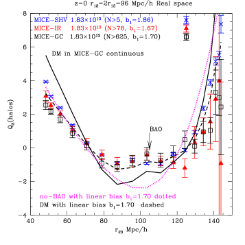
Figure 14 shows a comparison of $Q^{h}_{3}$ in halos of mass $M_{h}>1.83\times 10^{13}\,h^{-1}\,{\rm M_{\odot}}$ (without Warren correction) from simulations with different mass resolution, as detailed in Table 1: MICE-GC in black squares, MICE-IR with red triangles and MICE-SHV with blue crosses. The simulation with intermediate resolution has 8 times less particles per halo than the one with higher resolution, while the lowest resolution has 125 fewer particles. Notice that in the later case we are using as few as $5$ particles per halo as threshold and yet $Q_{3}$ has a very reasonable shape. In addition to the measured $Q^{h}_{3}$ we include $Q_{3}$ for the dark-matter in MICE-GC (solid black) and a linearly biased version $Q_{3}/b_{1}$ (dashed black), see Eq. (5). The dotted magenta is a similar estimate but assuming a theory $Q_{3}$ derived from a power spectrum with no wiggles. The figure focuses on large scales ($r_{12}=2r_{13}=96\,h^{-1}\,{\rm Mpc}$) and the BAO peak is clearly detected at $r_{23}\approx 110\,h^{-1}\,{\rm Mpc}$.

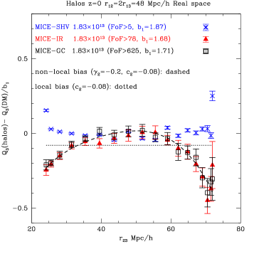
The differences between MICE-GC and MICE-IR are marginal, with derived linear bias values that agree at the percent level as found in Sec. 4.1 for well resolved halos. In turn MICE-SHV yield larger differences showing that such a low resolution is inappropriate for percent level accuracy studies. One subtlety is that even at the level of dark-matter there are some differences among these simulations, as discussed in Paper I. Figure 15 shows the effect of resolution on nonlinear bias by plotting $Q^{h}_{3}-Q^{dm}_{3}/b_{1}$ where both $Q_{3}^{h}$ and $Q^{dm}_{3}\equiv Q_{3}$ are measured in each given run. Thus we subtract the linear bias which also has some resolution coming effects coming from the DM. Moreover we focus on smaller scales, $r_{12}=2r_{13}=48\,h^{-1}\,{\rm Mpc}$. In Fig. 15 the local bias model corresponds to an horizontal line set by the non-linear bias $c_{2}$ while the non-local model of Chan et al. (2012) is given by the dashed black line. For isosceles triangles ($r_{23}=48\,h^{-1}\,{\rm Mpc}$) all three simulations agree, but for collapsed and elongated shapes MICE-SHV exceeds considerably the other two runs. In fact, while MICE-GC and MICE-IR track well the non local model clearly deviating from a horizontal line, MICE-SHV seems to be consistent with it for $c_{2}\sim 0$ (in addition to $\gamma_{2}=0$). Further work regarding higher order halo bias in MICE-GC computed with different methods can be found in Hoffmann et al. (2015).

Figure 15: Amplitude of the reduced 3-point function relative to the dark matter one measured in each run. Note how MICE-GC and MICE-IR agree with each other and with the non-local model. In turn, the MICE-SHV yield differences of few percent and seems to follow the local model (dotted line)

Figure 16: Halo bias in MICE-GC for 3 different mass threshold samples (as labeled). The shaded regions indicates a $1\%$ around the mean value measured at $r>30\,h^{-1}\,{\rm Mpc}$. For an $M_{\star}$-like sample the bias from halo-matter correlations (red symbols) is very close to scale-independent from small to large scales. At small scales ($r\lesssim 20\,h^{-1}\,{\rm Mpc}$) there is a clear trend of the clustering with increasing halo mass (with $b_{hm}\equiv\xi_{hm}/\xi_{mm}$ being smaller, similar and larger than the large-scale value). Across the BAO region there is slight clustering decrement ($\sim 2\%$) at $100\,h^{-1}\,{\rm Mpc}$ for the least massive halos and a clustering excess of $\sim 4-5\%$ at the BAO peak position (marked with a vertical arrow) for the most massive ones. For clarity error bars are only displayed for bias derived from $\xi_{hh}$.

5 Halo and Galaxy Bias from small to large (BAO) scales

As recalled in the introduction, one of the most interesting aspects of the MICE-GC run and its derived products is the combination of large volume and good mass resolution. In this section we profit from these by looking in detail at the scale dependence of halo and galaxy bias in configuration space, from small scales relevant for full-shape fitting (Sánchez et al., 2009, 2013, 2014) to large scales tracing the BAO feature (Anderson et al. (2012) and references therein).

In Fig. 16 we show the halo bias from two point correlation functions for three “mass threshold” halo samples, $M_{h}/(\,h^{-1}\,{\rm M_{\odot}})>5\times 10^{11},5\times 10^{12}$ and $7\times 10^{13}$. These samples were selected to have low, mid and high bias (top to bottom panels respectively). On the one hand Fig. 16 focuses on the comparison of the bias from the halo cross-correlation signal with dark-matter ($b=\xi_{hm}/\xi_{mm}$, red line) versus the one from halo auto-correlation ($b=(\xi_{hh}/\xi_{mm})^{1/2}$, blue line). On the other hand the panels split the bias measurement into small scales (shown with logarithmic binning) and large-scales (shown with linear binning). This is useful to determine on what scales the cross-correlation coefficient $r_{cc}\equiv\xi_{hm}/\sqrt{\xi_{mm}\xi_{hh}}$ departs from unity, a point that is typically linked to the brake-down of a local and deterministic biasing (Tegmark & Peebles, 1998; Dekel & Lahav, 1999). In each panel the filled region shows $1\%$ of the mean linear bias defined as the error weighted average over scales $s\geq 30\,h^{-1}\,{\rm Mpc}$. Defined in this way we find $b_{1}=0.95,1.28$ and $2.43$ (top to bottom). Both, Figs. 16 and 18, correspond to comoving catalogues at $z=0$. Error bars in those figures were obtained using jack-knife resampling with ${\rm njk}=64$ regions (measuring the bias in each region and the mean and variance weighted by ${\rm njk}-1$ afterwards).

Overall the halo bias is remarkably close to scale independent within few percent from large scales down to $15-20\,\,h^{-1}\,{\rm Mpc}$, with the cross correlation coefficient $r_{cc}$ being close to unity on this regime. On the largest scales there are however some residual effects worth highlighting.

For the least massive halos there seems to be a decrement of clustering amplitude around $100\,h^{-1}\,{\rm Mpc}$, although with a marginal amplitude of about $2\%$. As we increase the sample mass to $M_{h}\;\raise 1.29167pt\hbox{$>$\kern-7.5pt\raise-4.73611pt\hbox{$\sim$}}\;M_{\star}$ (see middle panel) the bias is consistent with linear bias almost within $1\%$. However for masses considerably above $M_{\star}$ (such as $M_{h}\geq 7\times 10^{10}\,h^{-1}\,{\rm M_{\odot}}$ as shown in the bottom panel of Fig. 16) we find an excess of clustering of $4\%-5\%$ precisely at the BAO peak ($r\approx 110\,h^{-1}\,{\rm Mpc}$ for our cosmology). This excess clustering increases with increasing mass, for $M_{h}\gtrsim 10^{14}\,h^{-1}\,{\rm M_{\odot}}$ is separately shown in Fig. 17. This pattern has been discussed by Desjacques et al. (2010) in the context of peak biasing and attributed for the most part to first order effects in Lagrangian Space, but more work is needed to characterize this as a function of mass and redshift.

At scales smaller than $20\,h^{-1}\,{\rm Mpc}$ the bias becomes steadily scale dependent due to nonlinear gravitational effects ($b_{2}$ terms in the language of PT) , again with an interesting dependence with mass since $b_{2}$ changes sign from negative to positive across the three halo samples shown (top to bottom respectively). Notice that this is the expected behavior for $b_{2}$ given the values of the linear bias $b_{1}$ at large scales (Cooray & Sheth, 2002).

At these scales the cross-correlation coefficient also departs from unity by up to $10\%$ at $r=5\,h^{-1}\,{\rm Mpc}$ (see also Sato & Matsubara (2013)). This is compatible with the emergence of nonlinear bias on these scales but might also signal a stochastic relation between halos and mass.

Figure 17: Scale dependence in bias across the BAO feature for a cluster mass scale halo sample. The sample is selected from the comoving output at $z=0$. Shaded regions as in Fig. 16. Error bars are only displayed for bias derived from halo auto-correlation for clarity, as in Fig. 16

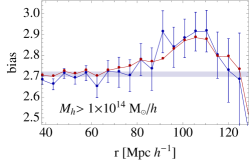
We next turn to investigate similar issues in the galaxy catalogue. Fig. 18 shows the galaxy bias from galaxy-mass cross correlations (red line) and from galaxy-galaxy auto-correlations for two distinctive samples. The top panel focuses on one faint magnitude limited sample ($M_{r}<-20.16$), already discussed in Sec. 2.2.1, for which the corresponding halo mass from the HOD+HAM mass-luminosity relation is $M_{h}\sim 10^{12}\,h^{-1}\,{\rm M_{\odot}}$. Bottom panel corresponds to a Luminous Red Galaxy sample defined through a bright absolute luminosity cut ($M_{r}<-21$) and one color cut $(g-r)>0.8$ (rest-frame colors). Both samples includes all galaxies, making no distinction between centrals and satellites, and hence populate in a non-trivial way a range of halo masses.

Figure 18: Scale dependence in galaxy bias for two samples in the MICE-GC comoving catalogue at $z=0$. Top panel correspond to an absolute magnitude limited sample ($M_{r}<-20.16$). Bottom panel to an LRG-like sample ($M_{r}<-21$ and $g-r>0.8$). The shaded region correspond to $1\%$ around the mean bias for $r>30\,h^{-1}\,{\rm Mpc}$. The panels show trends resembling those present for halo clustering. The $M_{r}<-20.16$ galaxies show a remarkably flat bias for $r>20\,h^{-1}\,{\rm Mpc}$ while the LRGs have a scale dependent feature across the BAO region of order $4-6\%$. Stronger nonlinear effects show up at smaller scales (for $r<20\,h^{-1}\,{\rm Mpc}$) but, contrary to the case of halos or centrals only shown in Fig. 16, the cross correlation coefficient remains close to unity down to $\sim{\rm few}\,h^{-1}\,{\rm Mpc}$ scales

The magnitude limited sample shows a bias remarkably close to scale independent across BAO scales and down to $r\sim 20\,h^{-1}\,{\rm Mpc}$, where nonlinear effects increase the clustering above the linear value. Notably the cross-correlation coefficients remains tightly close to unity all the way to $r\sim 5\,h^{-1}\,{\rm Mpc}$, a clear and remarkable difference with respect to the halos in Fig. 16. In a follow up work we will explore to what extent this depends on the satellite profiles or the halo exclusion. But for instance notice that our satellite galaxies do not necessarily follow the distribution of matter as we place them using a pre-determined profile.

Turning to the LRG sample in the bottom panel of Fig. 18 we find a clear scale dependent bias across the BAO feature, with an excess power at the BAO peak of about $5\%$ and a small $2\%$ deep at $80<r/(\,h^{-1}\,{\rm Mpc})<100$. A more detailed characterization of these effects as well as an interpretation from the theory point of view is left for further work. We note however that this kind of scale dependent residuals across BAO scales is relevant for an accurate calibration of the standard ruler test. We also note that our results are in qualitative agreement with other work in the literature (e.g. Angulo et al. (2014); Mehta et al. (2011); Padmanabhan & White (2009)).

6 Redshift Space Distortions

In this section we will discuss the properties of our galaxy catalogue in redshift space, which is a measure of how galaxy velocities are assigned.

6.1 Kaiser Limit and bias in the Lightcone

In the large-scale linear regime and in the plane-parallel approximation (where galaxies are taken to be sufficiently far away from the observer that the displacements induced by peculiar velocities are effectively parallel), the distortion caused by coherent infall velocities takes a particularly simple form in Fourier space (Kaiser, 1984):

$$\delta^{(s)}(k,\mu)=(1+f\mu^{2})\delta_{m}(k)$$ (6)

where $\mu$ is the cosine of the angle between $k$ and the line-of-sight, the superscript $s$ indicates redshift space, and $f(z)$ is given by,

$$f(z)\equiv\frac{d\;ln\;D}{d\;ln\;a}.$$ (7)

The second term in Eq. (6) is caused by radial peculiar velocities. If we assume that galaxy fluctuations are linearly biased by a factor $b$ relative to the underlying matter density $\delta_{m}$ (i.e. $\delta_{G}=b\,\delta_{m}$) but velocities are unbiased, then

$$\delta^{(s)}_{G}(k,\mu)=(b+f\mu^{2})\delta_{m}(k)$$ (8)

where $\delta^{(s)}_{G}$ are the measured galaxy fluctuations in redshift space. We then have an anisotropic power spectrum:

$$P^{(s)}_{gg}(k,\mu)=<(\delta^{(s)}_{G}(k))^{2}>=(b+f\mu^{2})^{2}P_{mm}(k)$$ (9)

where $P_{mm}(k)=<\delta^{2}_{m}(k)>$ is the real space matter power spectrum. This can be Fourier transformed and averaged over angles to obtain the monopole correlation function:

$$\xi_{gg} \equiv \xi_{\ell=0,gg}=K_{\ell=0}(z)~{}\xi_{mm}$$

$$\indent K_{\ell=0}(z) \equiv b(z)^{2}+\frac{2}{3}b(z)f(z)+\frac{1}{5}f(z)^{2}b(z)^{2}$$ (10)

where $\xi_{mm}$ is the matter correlation function at redshift $z$ (i.e. in linear theory $\xi_{mm}=D^{2}(z)\xi_{\rm L}(r,z=0)$) and we have defined $K_{0}(z)$ to be the monopole “linear Kaiser” factor.

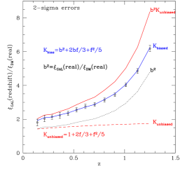
Figure 19 shows the ratio $\xi_{gg}/\xi_{mm}$ measured in the MICE-GC galaxy lightcone catalogue (error weighted averaged on scales $r>30\,h\,{\rm Mpc}^{-1}$) for an apparent magnitude limited sample ($r<24$). We compare it to the linear Kaiser factor $K$, where we use $b(z)$ as measured in real space and $f(z)$ given by the MICE cosmology. Note how both $b(z)$ and $f(z)$ change with redshift and that the predictions depend strongly on both ($b$ or $f$ alone cannot account for the observed variations, as indicated by red and dotted lines). There is an excellent agreement with the linear Kaiser model (in blue) for all redshifts and for the concrete bias evolution that results from cutting galaxies to $r<24$. On the one hand this serves as an excellent validation of the large-scale bulk galaxy velocities in the catalogue (which in turn are based on halo velocities). On the other hand, it means that both bias $b(z)$ and $f(z)$ can be constrained from observations using this simple modeling.

6.2 RSD for Central and Satellite Galaxies

In the previous section we showed that the Kaiser limit is a good model to describe the large-scale ($s\geq 30\,h^{-1}\,{\rm Mpc}$) clustering amplitude of the monopole correlation function and its lightcone evolution, provided with the bias as a function of redshift. In this section we investigate the break down of this large-scale limit due to the departure from purely bulk motions, in particular the impact of satellite galaxies.

We will focus on the multipole moments of the anisotropic galaxy power spectrum in redshift space,

$$P^{(s)}_{gg,\ell}(k)=\frac{2\ell+1}{2}\int_{-1}^{1}P^{(s)}_{gg}(k,\mu)L_{\ell}(\mu)d\mu$$ (11)

with $L_{\ell}$ being the Legendre polynomials. On large scales we can assume the “linear” relation in Eq. (9) and obtain the corresponding Kaiser limits : $P^{(s)}_{gg,\ell}(k)=K_{\ell}(b,f)P_{mm}(k)$, where $K_{0}$ is given in Eq. (10) and,

$$\indent\indent K_{2}(b,f) \equiv \frac{4}{3}bf+\frac{4}{7}f^{2}$$

$$K_{4}(b,f) \equiv \frac{8}{35}f^{2}$$ (12)

Figure 20 shows the first three moments, monopole ($\ell=0$), quadrupole ($\ell=2$) and hexadecapole ($\ell=4$) for the magnitude limited sample of galaxies discussed in Sec. 3.2, i.e. $M_{r}<-20.16$, in the comoving catalogue at $z=0$. In the mean, this luminosity corresponds to halos more massive than $10^{12}\,h^{-1}\,{\rm M_{\odot}}$. In order to understand what is the impact in the anisotropy of large-scale fluctuations from the motion of satellite galaxies inside halos we split the sample into “centrals only” (i.e. bulk motion of halos only), shown by red filled dots, and “all galaxies” (central plus satellites) shown by blue empty triangles. For this sample the satellite fraction is $24\%$. The corresponding multipole spectra for dark-matter is shown by dashed black lines.

Figure 19: Ratio of galaxy monopole 3D correlations in redshift space to the matter correlation in real space (points with errors), see Eq. (10). Dashed line shows the unbiased Kaiser prediction, while dotted line shows the bias measured in real space averaging over scales $s\geq 30\,h^{-1}\,{\rm Mpc}$. The blue line corresponds to the linear Kaiser model in Eq. (10) with this measured bias. This correspond to $r<24$ galaxies in the MICE-GC lightcone catalogue.

On the largest scales the Kaiser limit (shown in short-dashed) is reached for both the “centrals only” sample and the “central+satellites”, although in a more limited range of scales for the later. Notice that the large-scale bias of these two samples is slightly different ($b_{cen}=0.98$ and $b_{cen+sat}=1.2$) because of the scatter in the mass-luminosity relation discussed in Sec. 3.2. Hence the different Kaiser asymptotics in the monopole and quadrupole panels of Fig. 20 (while $K_{4}$ does not depend on bias). In turn, at $k<0.05\,h\,{\rm Mpc}^{-1}$ sampling variance dominates the hexadecapole results, despite the large simulation size. For reference we show the corresponding cosmic variance error assuming the multipole moments in redshift space to be Gaussian random fields (e.g. Taruya et al. (2009) and references therein).

Figure 20: The first 3 multipole power spectra for a magnitude limited galaxy sample ($M_{r}<-20.16$) at $z=0$. In each panel the corresponding $P_{\ell}$ has been divided by the measured (non-linear) matter power spectrum. The figure shows the case for central galaxies only, or the full sample (cen+sat) as well as the corresponding dark-matter. Hence it stresses the significant impact of satellite galaxies into the anisotropic clustering, basically by adding velocity dispersion. Notice how in all cases the Kaiser limit (short dashed line) is reached but only for the largest scales.

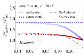
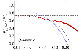
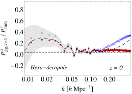
This is in contrast to the monopole or quadrupole, which can be measured to much smaller $k$, and results from the stronger dependence in the shape ($\mu^{4}$).

In order to investigate departures from the Kaiser limit we fit the following model to our monopole and quadrupole measurements (Scoccimarro, 2004),

$$P^{(s)}(k,\mu)=\left[b^{2}P_{\delta\delta}+2bf\mu^{2}P_{\delta\theta}+f^{2}\mu^{4}P_{\theta\theta}\right]\times{\rm e}^{-(k\mu f\sigma_{v})^{2}}$$ (13)

where we take $b$ to be the large-scale linear bias measured in real space (i.e. with a fixed value), $f=0.46$ for our cosmology at $z=0$ and $\sigma_{v}$ is a nuisance parameter related to (1D) velocity dispersion. In Eq. (13) $P_{XY}$ are the nonlinear density ($\delta$) and velocity divergence ($\theta$) auto and cross power spectra which we compute using MPTbreeze (Crocce et al., 2012). We stress that Eq. (13) is not expected to give accurate results but it is useful to hint on departures from the simplest linear Kaiser model discussed before.

From the monopole and quadrupole in Fig. 20 we find the best-fit to be $\sigma_{v}=6\,h^{-1}\,{\rm Mpc}$ for dark matter (equivalent to $600\,{\rm km/s}$), very close to the linear value

$$\sigma_{v,\rm Lin}=\left(\frac{4\pi}{3}\int P_{Lin}(q)dq\right)^{1/2}=6.15\,h^{-1}\,{\rm Mpc},$$ (14)

in agreement with Taruya et al. (2010). The “centrals” only sample (or halos) yields a smaller value $\sigma_{v}^{cen}=3\,h^{-1}\,{\rm Mpc}$ characteristic of a more coherent bulk motion. In turn the inclusion of satellite galaxies leads to virialized motions closer to those of dark matter, with a best-fit $\sigma_{v}^{all}=8.5\,h^{-1}\,{\rm Mpc}$.

6.3 Changing the velocity dispersion of satellite galaxies

As we discussed in Sec. 3.1 the spatial distribution of satellite galaxies is set by observational constraints from projected clustering (Carretero et al., 2015). However equivalent observational constraints for the distribution of satellite velocities are not that well stablished, hence our choice arises from well known results using hydrodynamical simulations (Bryan & Norman, 1998). In this section we study quantitatively how this assumption impact the anisotropic clustering.

Our procedure is to give the satellite galaxies the bulk motion of the halo plus an additional virial motion that follows a Gaussian distribution (in each axis) with a velocity dispersion $\sigma_{vir}=\langle v_{vir}^{2}\rangle\propto M^{2/3}_{h}$ (Sheth & Diaferio, 2001), so $v=v_{h}+v_{vir}$ where $v_{h}$ is the halo center of mass velocity (also the one of the central galaxy).

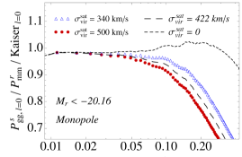
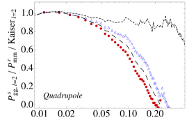
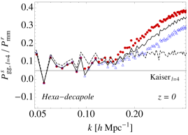
For the magnitude limited sample $M_{r}<-20.16$ discussed in Sec. 6 the velocity dispersion of satellites is $422\,{\rm Km\,sec^{-1}}$ (the distribution is narrower than a Gaussian, because it arises from a range of halo masses) while the satellite fraction is $\sim 30\%$. In Fig. 21 we show how the monopole, quadrupole and hexadecapole change when the satellite velocity dispersion is changed by $\pm 20\%$ keeping the bulk motion of the halos unaltered. As expected increasing the satellite velocity dispersion to $500\,{\rm km/s}$ induces more FoG effects (from satellite-central correlations in different halos) and a stronger scale dependent suppression of power. The monopole is suppressed at the $5\%$ level on scales $k\sim 0.15\,h\,{\rm Mpc}^{-1}$ compared to the fiducial case, while the quadrupole is more affected ($20\%$ at the same scale). In turn the hexa-decapole is too noisy on these scales, but the impact is clearly stronger. Reducing the satellite velocity dispersion to $340\,{\rm km/sec}$ (i.e. by $20\%$ less w.r.t the fiducial) has the opposite effects. We have done a more extreme case in which all satellites move with the bulk motion of the halo (setting $v_{vir}=0$). This is shown by short-dashed lines in Fig. 21. The result is that the anisotropic clustering in this case is well described by the simple linear Kaiser effect down to smaller scales.

Overall we find that satellite galaxies give a significant contribution to the anisotropic clustering through nonlinear redshift space distortions even on quite large-scales (see also Hikage & Yamamoto (2013); Masaki et al. (2013); Nishimichi & Oka (2014) for the case of LRG’s), yielding velocity dispersion effects similar (or larger) to those of dark-matter.

Figure 21: Change in the first 3 multipole power spectra for a magnitude limited galaxy sample ($M_{r}<-20.16$) when the virialized motion of satellite galaxies within the host halos is changed by $\sim\pm 20\%$. We normalized the measurements by the corresponding Kaiser prediction and the measured dark matter spectrum. The short dashed line corresponds to the extreme case where all satellite galaxies move with the bulk motion of their host halos.

7 Public Galaxy Catalogue Release

Together with this series of papers we make a first public data release of the current version of the MICE-GC lightcone catalogue (MICECAT v1.0). The halo and galaxy catalogue can be obtained at http://cosmohub.pic.es, a dedicated database portal hosted by Port d’Informació Científica (PIC). It corresponds to one octant of the full sky ($5000\,{\rm deg}^{2}$) from $z=0$ to $z=1.4$. In the current version (v1.0) galaxies are limited in absolute magnitude to $M_{r}<-18.9$ and halos in mass to $M_{h}>2.2\times 10^{11}\,h^{-1}\,{\rm M_{\odot}}$. Among other properties we provide angular positions and observed redshifts for all galaxies, flags to central/satellite distinctions, host halo masses, peculiar velocities, comoving distances, observed magnitudes (and magnitude errors) in several bands for surveys such as SDSS, DES and VISTA. Besides, we provide the SED template and dust extinction assigned to each galaxy which rely on the template library of Ilbert et al. (2009). These SEDs were used to generate the observed magnitudes. We also provide lensing information for each galaxy such as shear and convergence, as well as magnified magnitudes and angular positions (described in Paper III). Lastly we provide photometric redshift errors and error distributions based on a photometric template code.

The web-portal is set up to facilitate the download of the data, either the full compressed catalogue or by querying particular regions of the sky or data columns.

8 Conclusions

We have presented the MICE-GC halo and galaxy catalogues built upon one the largest N-body runs completed to date: the MICE Grand Challenge lightcone simulation. This N-body run contains about 70 billion particles in a 3 $\,h^{-1}\,{\rm Gpc}$ periodic box, a unique combination of large volume and fine mass resolution sampling 5 orders of magnitude in dynamical range.

We identify bound structures using a Friends-of-Friends algorithm with linking length $b=0.2$. Halos were resolved down to few times $10^{11}\,h^{-1}\,{\rm M_{\odot}}$ with a total of about $157$ million identified in each octant of the full sky lightcone up to $z=1.4$. A similar procedure was followed in several comoving outputs. We then populated the dark-matter halos with galaxies following a hybrid HOD and HAM scheme, matching the luminosity, color distributions and projected clustering properties (as a function of luminosity and g-r color) of SDSS galaxies at low-$z$. Lastly galaxy properties were evolved into the past lightcone using stellar evolution models. In all, this resulted in a catalogue limited in absolute magnitude to $M_{r}<-18.9$ and containing $\sim 2\times 10^{8}$ galaxies (considering only one octant of the full sky and $z<1.4$).

We have performed several validation tests of the catalogues, with the following main conclusions,

• Halo Catalogue: We showed that the halo mass function at $z=0$ agrees at the $1\%-2\%$ level with the Crocce et al. (2010) fit for well resolved halos (similarly for other comoving redshifts and the lightcone, were the fit does not assume universality). The cumulative abundance of groups with as low as 10 particles is up to $15\%$ below the model prediction using the Crocce et al. (2010) fit (which is a numerical fit calibrated to higher-resolution runs). In turn, the MICE-GC resolution and volume allow us to study halo clustering with good precision for samples with a broad range of linear bias values, even $b\lesssim 1$. The PBS prediction for this low bias sample agrees at the $2\%$ level with the bias measured from $P_{hm}/P_{mm}$, a better performance than for massive objects (Manera et al., 2010). We note that this regime of low-bias was not well explored previously and deserves a more detailed analysis for more robust conclusions about the performance of PBS. Lastly, halos in the lightcone presented an almost constant clustering amplitude, i.e. degenerate with the growth factor evolution, for constant mass samples. Instead, galaxies selected above an apparent luminosity threshold show a clustering amplitude that increases with redshift.
  

• Galaxy Catalogue: Starting from fits at low redshift and implementing evolutionary corrections to galaxies and resampling SEDs from COSMOS (Ilbert et al., 2009), we were able to predict the color distributions and clustering properties of higher-redshift galaxy populations ($0.8<z<1.4$). In particular, MICE and COSMOS galaxies have very similar color-color distributions at low-$z$, whereas the MICE sample is slightly bluer at higher redshifts, as depicted by Fig. 7. As for the clustering, MICE mock galaxies match very well the shape of the angular correlation function of COSMOS galaxies at $z=0.6$ for a sample brighter than $i_{AB}<22.5$. A similar match is found at $z=1$ for galaxies with $i_{AB}<24$, except for the rise in clustering strength in COSMOS at angular scales larger than 5 arc minutes, which we attribute to the known excess of clustering power in the COSMOS field (Skibba et al., 2014). Compared to the dark matter the galaxy clustering of these samples is consistent with a simple linear bias model with $b\sim 1.16$ and $b\sim 1.8$ respectively, for scales $\theta\gtrsim$ 1 arc minute (see Figs. 8 and 9). We also built a sample resembling the DR10-BOSS CMASS sample of LRGs which implied doing a magnitude and color selection over MICE-GC galaxies. The resulting redshift distribution and clustering (monopole and quadrupole) were in good agreement with the corresponding measurements in DR10.

We have then explored some concrete applications for these catalogues. The main findings in this regard are as follows:

• We have studied how the large-scale halo clustering depends on the mass resolution of the underlying N-body simulation. We focused first in the halo-matter cross-power spectrum which is a robust measure of halo clustering against shot noise. Using this estimator we find the bias to be up to $5\%$ larger for halos resolved with $20-50$ particles in our MICE-IR run than for the corresponding sample in MICE-GC (a factor of 8 more particles), and $10\%$ for $10-20$ particle halos. The exact value depends on whether halo masses are corrected for discreteness following Warren et al. (2006) or not (for poorly resolved halos the applicability of this correction is unclear and makes the effect worse). For well resolved halos we find no significant difference between MICE-IR and MICE-GC large scale clustering. Although we concentrated in the comoving output at $z=0.5$ we have reached similar conclusions at $z=0$.
  

• We also looked into this effect in higher order statistics by measuring the reduced 3-point function, $Q_{3}$, of massive halos $M_{h}\geq 1.83\times 10^{13}\,h^{-1}\,{\rm M_{\odot}}$ (sampled with $N_{p}\geq 625$ in MICE-GC, $N_{p}\geq 78$ particles in MICE-IR and only $5$ particles in MICE-SHV) at $z=0$. Mass resolution effects for this halo resolution do not affect the shape of the 3-point function unless we use extremely low resolution as for MICE-SHV. Although the MICE-SHV halos yield the correct shape for $Q_{3}$ there are few percent level differences. For smaller scales MICE-GC and MICE-IR deviate clearly from the simple local model and track well the non-local prediction from Chan et al. (2012), see Fig. 14.
  

• We investigated scale dependent bias from small (few $\,h^{-1}\,{\rm Mpc}$) to large BAO scales (up to $\sim 130\,h^{-1}\,{\rm Mpc}$) in the two-point correlation function of halos and galaxies at $z=0$. We focused on three halo mass threshold samples, $M_{h}/(\,h^{-1}\,{\rm M_{\odot}})\geq 5\times 10^{11},5\times 10^{12}$ and $7\times 10^{13}$, and found the bias to be remarkably close to scale independent (within $2\%$) for scales $20\lesssim r/(\,h^{-1}\,{\rm Mpc})\lesssim 80$. For the intermediate mass scale (roughly $M_{\star}$ halos) the bias is flat also across the BAO. However for more massive halos we find an excess of clustering at BAO scales of $\sim 5\%$, while for less massive objects we instead find an almost marginal decrement of clustering amplitude of $\sim 3\%-4\%$ at $80\lesssim r/(\,h^{-1}\,{\rm Mpc})\lesssim 110$. Stronger nonlinear effects show up at scales of $r<20\,h^{-1}\,{\rm Mpc}$ together with departures of the cross-correlation coefficient $r_{cc}$ from unity. We then investigated how this translates to the clustering of galaxies, which as a non-trivial combination of the one of halos through the HOD. For a faint luminosity cut $M_{r}<20.16$, corresponding to an $L_{\rm cen}=L_{\rm cen}(M_{h})$ relation of $M_{h}\sim 10^{12}\,h^{-1}\,{\rm M_{\odot}}$, we find the bias to be constant with scale for $r>20\,h^{-1}\,{\rm Mpc}$. In turn, for an LRG type selection (bright $M_{r}<-21$ and red $g-r>0.8$ galaxies) we again find a non-trivial scale dependent bias across the BAO feature of about $6\%-8\%$. For galaxies, we find the cross-correlation coefficient close to unity down to few $\,h^{-1}\,{\rm Mpc}$. Overall these are relevant conclusions for standard ruler tests that aims to extract distance-redshift relations from galaxy clustering (as they impact the observed BAO feature) or for modeling the full-shape of the correlation function. We leave a more detailed analysis for follow-up work.
  

• Lastly we studied galaxy clustering in redshift space, a testing ground for galaxy peculiar velocities. Using the lightcone we find the averaged amplitude of the monopole correlation function on scales $r>30\,h^{-1}\,{\rm Mpc}$ to be very consistent with the linear Kaiser model (with an input bias from real-space measurements). This was true across all redshifts sampled in the lightcone ($z<1.4$) which is a non-trivial test of both $b(z)$ and $f(z)$. We next looked into departures from the linear Kaiser model in the multipole moments of the galaxy anisotropic power spectrum at the $z=0$ snapshot. While on large scales all multipoles agree with the Kaiser limit there are departures already at $k\sim 0.05\,h\,{\rm Mpc}^{-1}$. Notably the satellite galaxies make the anisotropic clustering stronger, in the sense of increasing Finger-of-God effects to reach (or surpass) those of dark-matter.
  

  In a series of three papers we introduce in detail the MICE-GC mock galaxy catalogue, the ending product of an elaborated step-by-step process that puts together dark-matter, halos, galaxies and lensing, with a strong observational angle. The success of the largest ongoing and future cosmological surveys is based upon our ability to develop suitable simulations for their analysis and science. We make our catalogue publicly available, with the aim of contributing to the community wide effort in shaping the upcoming era of precision cosmology.

References

- Anderson et al. (2012) Anderson L., Aubourg E., Bailey S., Bizyaev D., Blanton M., Bolton A. S., Brinkmann J., Brownstein J. R., Burden A., et al., 2012, MNRAS , 427, 3435
- Angulo et al. (2014) Angulo R. E., Baugh C. M., Frenk C. S., Lacey C. G., 2014, MNRAS , 442, 3256
- Angulo et al. (2014) Angulo R. E., White S. D. M., Springel V., Henriques B., 2014, MNRAS , 442, 2131
- Astier et al. (2006) Astier P., Guy J., Regnault N., Pain R., Aubourg E., Balam D., Basa S., Carlberg R. G., Fabbro S., Fouchez D., et al., 2006, A&A , 447, 31
- Bardeen et al. (1986) Bardeen J. M., Bond J. R., Kaiser N., Szalay A. S., 1986, Astrophys. J. , 304, 15
- Bennett et al. (2003) Bennett C. L., Halpern M., Hinshaw G., Jarosik N., Kogut A., Limon M., Meyer S. S., Page L., Spergel D. N., Tucker G. S., et al., 2003, Astrophys. J. Suppl. , 148, 1
- Berlind & Weinberg (2002) Berlind A. A., Weinberg D. H., 2002, Astrophys. J. , 575, 587
- Bhattacharya et al. (2011) Bhattacharya S., Heitmann K., White M., Lukić Z., Wagner C., Habib S., 2011, Astrophys. J. , 732, 122
- Blanton et al. (2003) Blanton M. R., Hogg D. W., Bahcall N. A., Baldry I. K., Brinkmann J., Csabai I., Eisenstein D., Fukugita M., Gunn J. E., Ivezić Ž., et al., 2003, Astrophys. J. , 594, 186
- Blanton et al. (2003) Blanton M. R., Hogg D. W., Bahcall N. A., Brinkmann J., Britton M., Connolly A. J., Csabai I., Fukugita M., Loveday J., Meiksin A., et al., 2003, Astrophys. J. , 592, 819
- Blanton et al. (2005) Blanton M. R., Schlegel D. J., Strauss M. A., Brinkmann J., Finkbeiner D., Fukugita M., Gunn J. E., Hogg D. W., Ivezić Ž., Knapp G. R., Lupton R. H., Munn J. A., Schneider D. P., Tegmark M., Zehavi I., 2005, AJ, 129, 2562
- Bryan & Norman (1998) Bryan G. L., Norman M. L., 1998, Astrophys. J. , 495, 80
- Bullock et al. (2001) Bullock J. S., Kolatt T. S., Sigad Y., Somerville R. S., Kravtsov A. V., Klypin A. A., Primack J. R., Dekel A., 2001, MNRAS , 321, 559
- Carretero et al. (2015) Carretero J., Castander F. J., Gaztañaga E., Crocce M., Fosalba P., 2015, MNRAS , 447, 646
- Chan et al. (2012) Chan K. C., Scoccimarro R., Sheth R. K., 2012, Phys. Rev. D , 85, 083509
- Cole & Kaiser (1989) Cole S., Kaiser N., 1989, MNRAS , 237, 1127
- Cole et al. (2005) Cole S., Percival W. J., Peacock J. A., Norberg P., Baugh C. M., Frenk C. S., Baldry I., Bland-Hawthorn J., Bridges T., Cannon R., et al., 2005, MNRAS , 362, 505
- Conroy et al. (2006) Conroy C., Wechsler R. H., Kravtsov A. V., 2006, Astrophys. J. , 647, 201
- Cooray & Sheth (2002) Cooray A., Sheth R., 2002, Phys. Rep. , 372, 1
- Crocce et al. (2010) Crocce M., Fosalba P., Castander F. J., Gaztañaga E., 2010, MNRAS , 403, 1353
- Crocce & Scoccimarro (2008) Crocce M., Scoccimarro R., 2008, Phys. Rev. D , 77, 023533
- Crocce et al. (2012) Crocce M., Scoccimarro R., Bernardeau F., 2012, MNRAS , 427, 2537
- Dekel & Lahav (1999) Dekel A., Lahav O., 1999, Astrophys. J. , 520, 24
- Desjacques et al. (2010) Desjacques V., Crocce M., Scoccimarro R., Sheth R. K., 2010, Phys. Rev. D , 82, 103529
- Feldman et al. (1994) Feldman H. A., Kaiser N., Peacock J. A., 1994, Astrophys. J. , 426, 23
- Fosalba et al. (2013) Fosalba P., Crocce M., Gaztanaga E., Castander F. J., 2013, ArXiv e-prints astro-ph/1312.1707
- Fosalba et al. (2015) Fosalba P., Gaztañaga E., Castander F. J., Crocce M., 2015, MNRAS , 447, 1319
- Frieman & Gaztanaga (1994) Frieman J. A., Gaztanaga E., 1994, Astrophys. J. , 425, 392
- Fry & Gaztanaga (1993) Fry J. N., Gaztanaga E., 1993, Astrophys. J. , 413, 447
- Groth & Peebles (1977) Groth E. J., Peebles P. J. E., 1977, Astrophys. J. , 217, 385
- Heitmann et al. (2014) Heitmann K., Lawrence E., Kwan J., Habib S., Higdon D., 2014, Astrophys. J. , 780, 111
- Hikage & Yamamoto (2013) Hikage C., Yamamoto K., 2013, JCAP , 8, 19
- Hoffmann et al. (2015) Hoffmann K., Bel J., Gaztañaga E., Crocce M., Fosalba P., Castander F. J., 2015, MNRAS , 447, 1724
- Ilbert et al. (2009) Ilbert O., Capak P., Salvato M., Aussel H., McCracken H. J., Sanders D. B., Scoville N., Kartaltepe J., Arnouts S., Le Floc’h E., et. al., 2009, Astrophys. J. , 690, 1236
- Jing et al. (1998) Jing Y. P., Mo H. J., Boerner G., 1998, Astrophys. J. , 494, 1
- Jing & Suto (2002) Jing Y. P., Suto Y., 2002, Astrophys. J. , 574, 538
- Kaiser (1984) Kaiser N., 1984, Astrophys. J. , 282, 374
- Lukić et al. (2009) Lukić Z., Reed D., Habib S., Heitmann K., 2009, Astrophys. J. , 692, 217
- Manera & Gaztañaga (2011) Manera M., Gaztañaga E., 2011, MNRAS , 415, 383
- Manera et al. (2013) Manera M., Scoccimarro R., Percival W. J., Samushia L., McBride C. K., Ross A. J., Sheth R. K., White M., Reid B. A., Sánchez A. G., et al., 2013, MNRAS , 428, 1036
- Manera et al. (2010) Manera M., Sheth R. K., Scoccimarro R., 2010, MNRAS , 402, 589
- Masaki et al. (2013) Masaki S., Hikage C., Takada M., Spergel D. N., Sugiyama N., 2013, MNRAS , 433, 3506
- Mehta et al. (2011) Mehta K. T., Seo H.-J., Eckel J., Eisenstein D. J., Metchnik M., Pinto P., Xu X., 2011, Astrophys. J. , 734, 94
- Nishimichi & Oka (2014) Nishimichi T., Oka A., 2014, MNRAS , 444, 1400
- Padmanabhan & White (2009) Padmanabhan N., White M., 2009, Phys. Rev. D , 80, 063508
- Perlmutter et al. (1999) Perlmutter S., Aldering G., Goldhaber G., Knop R. A., Nugent P., Castro P. G., Deustua S., Fabbro S., Goobar A., Groom D. E., Supernova Cosmology Project 1999, Astrophys. J. , 517, 565
- Planck Collaboration et al. (2014) Planck Collaboration Ade P. A. R., Aghanim N., Armitage-Caplan C., Arnaud M., Ashdown M., Atrio-Barandela F., Aumont J., Baccigalupi C., Banday A. J., et al., 2014, A&A , 571, A16
- Riess et al. (1998) Riess A. G., Filippenko A. V., Challis P., Clocchiatti A., Diercks A., Garnavich P. M., Gilliland R. L., Hogan C. J., Jha S., Kirshner R. P., et al., 1998, Astronom. J. , 116, 1009
- Sánchez et al. (2009) Sánchez A. G., Crocce M., Cabré A., Baugh C. M., Gaztañaga E., 2009, MNRAS , 400, 1643
- Sánchez et al. (2013) Sánchez A. G., Kazin E. A., Beutler F., Chuang C.-H., Cuesta A. J., Eisenstein D. J., Manera M., Montesano F., Nichol R. C., Padmanabhan N., et al., 2013, MNRAS , 433, 1202
- Sánchez et al. (2014) Sánchez A. G., Montesano F., Kazin E. A., Aubourg E., Beutler F., Brinkmann J., Brownstein J. R., Cuesta A. J., Dawson K. S., Eisenstein D. J., et al., 2014, MNRAS , 440, 2692
- Sato & Matsubara (2013) Sato M., Matsubara T., 2013, Phys. Rev. D , 87, 123523
- Scoccimarro (2004) Scoccimarro R., 2004, Phys. Rev. D , 70, 083007
- Scoccimarro et al. (2001) Scoccimarro R., Sheth R. K., Hui L., Jain B., 2001, Astrophys. J. , 546, 20
- Sheth & Diaferio (2001) Sheth R. K., Diaferio A., 2001, MNRAS , 322, 901
- Sheth & Tormen (1999) Sheth R. K., Tormen G., 1999, MNRAS , 308, 119
- Skibba et al. (2014) Skibba R. A., Smith M. S. M., Coil A. L., Moustakas J., Aird J., Blanton M. R., Bray A. D., Cool R. J., Eisenstein D. J., Mendez A. J., Wong K. C., Zhu G., 2014, Astrophys. J. , 784, 128
- Smith et al. (2007) Smith R. E., Scoccimarro R., Sheth R. K., 2007, Phys. Rev. D , 75, 063512
- Takahashi et al. (2012) Takahashi R., Sato M., Nishimichi T., Taruya A., Oguri M., 2012, Astrophys. J. , 761, 152
- Taruya et al. (2010) Taruya A., Nishimichi T., Saito S., 2010, Phys. Rev. D , 82, 063522
- Taruya et al. (2009) Taruya A., Nishimichi T., Saito S., Hiramatsu T., 2009, Phys. Rev. D , 80, 123503
- Tasitsiomi et al. (2004) Tasitsiomi A., Kravtsov A. V., Wechsler R. H., Primack J. R., 2004, Astrophys. J. , 614, 533
- Tegmark & Peebles (1998) Tegmark M., Peebles P. J. E., 1998, Astrophys. J. Lett. , 500, L79
- Tegmark et al. (2004) Tegmark M., Strauss M. A., Blanton M. R., Abazajian K., Dodelson S., Sandvik H., Wang X., Weinberg D. H., Zehavi I., Bahcall N. A., et al., 2004, Phys. Rev. D , 69, 103501
- The Dark Energy Survey Collaboration (2005) The Dark Energy Survey Collaboration 2005, ArXiv e-prints astro-ph/0510346
- Tinker et al. (2010) Tinker J. L., Robertson B. E., Kravtsov A. V., Klypin A., Warren M. S., Yepes G., Gottlöber S., 2010, Astrophys. J. , 724, 878
- Tojeiro et al. (2012) Tojeiro R., Percival W. J., Wake D. A., Maraston C., Skibba R. A., Zehavi I., Ross A. J., Brinkmann J., Conroy C., Guo H., et al., 2012, MNRAS , 424, 136
- Vale & Ostriker (2004) Vale A., Ostriker J. P., 2004, MNRAS , 353, 189
- Warren et al. (2006) Warren M. S., Abazajian K., Holz D. E., Teodoro L., 2006, Astrophys. J. , 646, 881
- Watson et al. (2012) Watson D. F., Berlind A. A., McBride C. K., Hogg D. W., Jiang T., 2012, Astrophys. J. , 749, 83
- White et al. (2014) White M., Tinker J. L., McBride C. K., 2014, MNRAS , 437, 2594
- York et al. (2000) York D. G., Adelman J., Anderson Jr. J. E., Anderson S. F., Annis J., Bahcall N. A., Bakken J. A., Barkhouser R., Bastian S., Berman E., et al. 2000, AJ, 120, 1579
- Zehavi et al. (2011) Zehavi I., Zheng Z., Weinberg D. H., Blanton M. R., Bahcall N. A., Berlind A. A., Brinkmann J., Frieman J. A., Gunn J. E., Lupton R. H., et al., 2011, Astrophys. J. , 736, 59