Charge and spin current in a quasi-one-dimensional quantum wire with spin-orbit coupling

Abstract

We show that Rashba spin-orbit coupling may result in an energy gap in the spectrum of electrons in a two-mode quantum wire if a suitable confining potential is chosen. This leads to a dip in the conductance and a spike in the spin current at the corresponding position of the Fermi level. Therefore one may control the charge and spin currents by means of electrostatic gates without using magnetic field or magnetic materials.

I Introduction

Spintronics, or spin electronics, involves the study of active control and manipulation of spin degrees of freedom in solid-state systems and is a rapidly growing field of science.Zutic04 The key purpose of these studies is the generation, control, and manipulation of spin-polarized currents. A useful tool for achieving this goal is the spin-orbit interaction, which couples the spin of an electron with its spatial motion in a presence of a certain asymmetry of the conductor. For example, Rashba spin-orbit interaction is due to a lack of inversion symmetry in semiconductor heterostructures such as InAs or GaAs.Rashba60 The advantage of this type of interaction is that it can be tuned by means of electrostatic gates.Nitta97 ; Engels97

In truly single-mode quantum channels, spin-orbit interaction alone neither changes the electric current nor results in a spin current if no magnetic field or magnetic materials are involved. In this case, spin-orbit interaction does not change the energy-band topology and can be simply eliminated from the Hamiltonian by means of a unitary transform.Levitov03

A prototypical scheme of a spin field-effect transistor based on Rashba interaction and single-mode ballistic channel with ferromagnetic electrodes was proposed by Datta and DasDatta90 more than two decades ago. Recently, such a device was experimentally realized.Koo09

The current in a single-mode quantum channel also depends on the spin-orbit interaction if a magnetic field is applied parallel to the channel or normally to the plane of the heterostructure (i.e. in the direction of Rashba field).Pershin04 The interplay of the spin-orbit interaction with magnetic field significantly modifies the band structure and produces an energy gap in the spectrum together with additional subband extrema. This results in a decrease in the charge current and a net spin current as the Fermi level passes through the gap. These effects were recently experimentally observed by Quay et al.Quay10

Many authors studied spin and charge transport in multimode quantum channels in the absence of magnetic field or magnetic ordering. Governale and ZülickeGovernale02 considered a long channel with parabolic confinement potential and took into account the mixing of different transverse-quantization subbands by the spin-orbit interaction. This mixing results in an asymmetric distortion of the dispersion curves but does not open any gaps in the spectrum. As a consequence, the spin-orbit interaction in a presence of voltage drop across the channel results in a spin accumulation inside the channel but does not lead to a spin current or deviations from the standard conductance quantization. There is also a number of numerical calculations of the spin current,Eto05 ; Zhai07 ; Liu07 ; Zhai08 but these papers deal with stepwise constrictions and the results are obscured by the interference effects. A more realistic geometry of a saddle-point contact in two-dimensional potential landscape was considered in Ref. Sablikov10, , but the Rashba interaction was taken into account there as a perturbation. In Refs. Sanchez06, and Gelabert10, , a quasi-one-dimensional wire with localized region of Rashba interaction was considered and nonzero spin current was predicted for sufficiently sharp boundaries of the region. Unusual trajectories were revealed by Silvestrov and MishchenkoSilvestrov06 within the quasiclassical approach to exist near these regions. However in all the above papers, the spin current and the deviations from perfect conductance quantization are related with the mixing of subbands in the transition areas between the quantum contact and reservoirs by spin-orbit interaction and crucially depend on the geometry and properties of these regions. It is hard to see any general regularities concerning the magnitude of the effect.

In this paper, we propose a mechanism of spin current generation that relies on the energy band structure deep in the wire rather than on the reflection effects in the transition areas and leads to 100% spin-polarized current at definite positions of the Fermi level. This mechanism is reminiscent of the one in Ref. Pershin04, but requires no magnetic field.

II The model

Consider a quasi-one-dimensional conducting channel formed in two-dimensional electron gas by means of electrostatic gates. The transition between the reservoirs and the channel is assumed to be adiabatic, and the length of the channel is much larger than that of the transition regions. We assume that the Rashba spin-orbit interaction is present in the channel but absent in the reservoirs, so the spin current through the system is well-defined. The Hamiltonian of the system is of the form

$$\hat{H}=\frac{\hat{p}^{2}_{x}}{2m}+\frac{\hat{p}^{2}_{z}}{2m}+U(x,z)\\ +\frac{\alpha(x)}{\hbar}\left(\hat{p}_{x}\hat{\sigma}_{z}-\hat{p}_{z}\hat{\sigma}_{x}\right)-\frac{i}{2}\,\frac{\partial\alpha}{\partial x}\,\hat{\sigma}_{z},$$ (1)

where $U(x,z)$ is the confining potential and $\alpha(x)$ is the parameter of spin-orbit coupling. Both quantities are smooth functions of the longitudinal coordinate $x$ that are constant almost throughout the whole length of channel and vanish in the reservoirs. It is now straightforward to make use of the adiabatic approximation and introduce a complete set of of eigenfunctions $\varphi_{n}(x,z)$ and eigenenergies $\varepsilon_{n}$ corresponding to the transverse motion of electrons in the $z$ direction. This leads to a set of coupled equations of the form

$$\left[\frac{\hat{p}_{x}^{2}}{2m}+\frac{\alpha(x)}{\hbar}\,\hat{\sigma}_{z}\,\hat{p}_{x}-\frac{i}{2}\,\frac{d\alpha}{dx}\,\hat{\sigma}_{z}+\varepsilon_{m}\right]\bar{\psi}_{m}(x)\\ -\frac{\alpha(x)}{\hbar}\,\hat{\sigma}_{x}\sum_{n}\langle m|p_{z}|n\rangle\,\bar{\psi}_{n}(x)=\varepsilon\,\bar{\psi}_{m}(x)$$ (2)

for the spinors $\bar{\psi}_{n}=(u_{n},\,v_{n})^{T}$ that describe the longitudinal dependence of the spin-up and spin-down amplitudes of wave-function in the $n$-th transverse quantum mode.

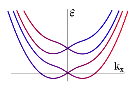
Figure 1: Dispersion curves for the two lowest subbands of a quantum wire with spin-orbit interaction and parabolic transverse confinement. The dispersion curves are distorted by level crossing but exhibit no local maxima.The color of the curve designates the dominant spin projection.

If the matrix elements of transverse momentum between different modes $\varphi_{m}$ and $\varphi_{n}$ were zero, the twofold spin degeneracy of these modes would be lifted by the spin-orbit interaction and one should see two sets of parabolic dispersion curves shifted along the $k_{x}$ axis that would correspond to the two possible projections of spin on the $z$ axis. The curves of each set would have minima at $k_{x}=\pm 2m\alpha/\hbar^{2}$ and intersect without affecting each other.

Nonzero matrix elements $\langle m|p_{z}|n\rangle$ result in anticrossing of the dispersion curves with different $n$ and spin projection and lead to an asymmetric distortion of them (see Fig. 1). However this does not give rise to new maxima and minima in these curves for the case of standard parabolic confining potential.Moroz99 The reason is that the levels of transverse quantization are evenly spaced and it is impossible to isolate a pair of them with a small separation. In other words, the vertical separation of anticrossing curves is too large as compared with their horizontal shifts.

The failure of the approximate two-band model that predicts a nonmonotonic behavior of the curves may be understood as follows. In the absence of band mixing, the two curves corresponding to two subsequent transverse-quantization levels and different spin projection would cross at $k_{x}=\Delta\varepsilon/2\alpha$, where $\Delta\varepsilon=\varepsilon_{n+1}-\varepsilon_{n}$. To form a maximum, the crossing branches of these curves should have different signs of slope $k_{x}+2m\alpha/\hbar^{2}>0$ and $k_{x}-2m\alpha/\hbar^{2}<0$ at the intersection point, which results in a condition $\Delta\varepsilon<4m\alpha^{2}/\hbar^{2}$. On the other hand, the band mixing term $\alpha\langle n+1|p_{z}|n\rangle/\hbar$ would lead to the splitting of the curves at the crossing point of the order of $\Omega\sim\sqrt{m\Delta\varepsilon}\,\alpha/\hbar$. The two-band model is justified only if $\Omega\ll\Delta\varepsilon$, i.e. $\Delta\varepsilon\gg m\alpha^{2}/\hbar^{2}$, which is incompatible with the previous condition. Exact calculationsGovernale02 show that all the dispersion curves have only one minimum and hence the dependence of the conductance of the channel on the Fermi energy exhibits only the conventional $2e^{2}/h$ steps, while the spin current is absent.

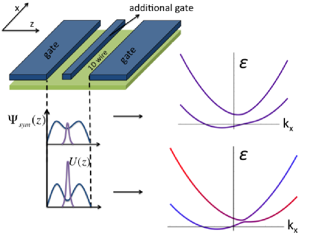
Figure 2: The system under consideration. The current flows in the $x$ direction, and the negative voltage at the additional middle gate changes the confining potential from one-well to a double-well shape. As the negative voltage increases, a maximum appears in the lower dispersion curve.

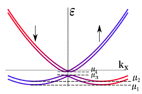
Figure 3: Dispersion curves for a pair of closely spaced energy levels with small matrix element of transverse momentum in a quantum wire with spin-orbit interaction. The level crossing results in appearance of local maxima in the lower curves.

Things become different if the confinement is nonparabolic. Consider, e. g., the system in which $U(z)$ has the shape of a double potential well. Such a potential may be formed by means of a negatively biased central gate on top of the quantum wire (see Fig. 2). In the case of a high impenetrable barrier between the wells, each of them would possess the same set of energy levels, so the levels of the whole system would be doubly degenerate. A finite tunneling through the barrier lifts the degeneracy, and therefore one gets a set of pairs of levels with very small spacings inside the pair. In this case, the two-band model is justified and taking into account only the two lowest levels, one obtains the following expression for the resulting dispersion curves

$$\varepsilon=\frac{\hbar k_{x}^{2}}{2m}+\frac{\varepsilon_{1}+\varepsilon_{2}}{2}\\ \pm\frac{1}{2}\sqrt{(\varepsilon_{2}-\varepsilon_{1}\pm 2\alpha k_{x})^{2}+4|p_{12}|^{2}\alpha^{2}/\hbar^{2}},$$ (3)

where $p_{12}=\langle 1|p_{z}|2\rangle$. The upper sign at $2\alpha k_{x}$ under the square root corresponds to the mixture of $|1\uparrow\rangle$ and $|2\downarrow\rangle$ states, and the lower sign corresponds to the mixture of $|1\downarrow\rangle$ and $|2\uparrow\rangle$ states. The two pairs of the resulting curves are symmetric with respect to $k_{x}=0$. The lower dispersion curve may have one or two minima as a function of $k_{x}$ depending on the relations between $\Delta\varepsilon=\varepsilon_{2}-\varepsilon_{1}$, $p_{12}$, and $\alpha$ (see Fig. 3). The upper minimum disappears by merging with the local maximum, i. e. when the points where $d\varepsilon/dk_{x}=0$ and $d^{2}\varepsilon/dk_{x}^{2}=0$ coincide. Therefore it follows from Eq. (3) that the second minimum exists if

$$\left|\frac{\hbar p_{12}}{m\alpha}\right|^{2/3}+\left(\frac{\hbar^{2}\Delta\varepsilon}{2m\alpha^{2}}\right)^{2/3}<1.$$ (4)

Apparently one can meet this condition by making the overlap of the wave functions in the two wells sufficiently small. For example, if a square quantum well with infinitely high external walls is symmetrically cut by a $\delta$-like barrier in the middle, both $\Delta\varepsilon$ and $|p_{12}|$ are inversely proportional to the effective strength of the barrier $k_{0}$.

III The conductance

The existence of a local maximum in the lower pair of the dispersion curves leads to significant changes in the conductance of the wire. If the Fermi level lies between the lower and upper minima $\mu_{1}$ and $\mu_{2}$ in the dispersion curves (see Fig. 3), it intersects two branches with positive (negative) group velocity that correspond to the two different spin projections in the $z$ direction, and the conductance is $2e^{2}/h$, while the spin current is absent. If the Fermi level lies between the upper minimum $\mu_{2}$ and the local maximum $\mu_{3}$ in the lower curves or above the minimum in the two upper dispersion curves $\mu_{4}$, it intersect two branches with positive (negative) group velocity and one spin projection and two branches with positive (negative) group velocity with the other spin projection. This results in the $4e^{2}/h$ conductance and yields no spin current. However if the Fermi level falls within the gap between the local maximum $\mu_{3}$ in the lower curves and the minimum $\mu_{4}$ in the upper curves, it intersect two branches with positive group velocities and one spin projection and two branches with negative velocities and the other spin projection. Therefore in the case of a sufficiently long wire the conductance exhibits a dip to $2e^{2}/h$ where the current is 100% spin polarized.

To calculate the current through the wire, we use the Landauer - Büttiker formulaButtiker85 for the zero-temperature total electric conductance

$$G=\frac{e^{2}}{h}\sum\limits_{n_{L},n_{R},\sigma_{L},\sigma_{R}}|t_{n_{R}\sigma_{R},n_{L}\sigma_{L}}|^{2}$$ (5)

where $t_{n_{R}\sigma_{R},n_{L}\sigma_{L}}$ are the transmission amplitudes from the state in transverse mode $n_{L}$ with spin projection $\sigma_{L}$ in the left lead to the state in the mode $n_{R}$ with spin projection $\sigma_{R}$ in the right lead. The spin conductance $G_{z}^{s}=I_{s}/V$ with respect to the $z$ axis is given byZhai05

$$G_{z}^{s}=-\frac{e}{4\pi}\sum\limits_{n_{L},n_{R},\sigma_{L}}\bigl{(}t^{*}_{n_{R}\uparrow,n_{L}\sigma_{L}}t_{n_{R}\uparrow,n_{L}\sigma_{L}}\\ -t^{*}_{n_{R}\downarrow,n_{L}\sigma_{L}}t_{n_{R}\downarrow,n_{L}\sigma_{L}}\bigr{)}.$$ (6)

In general, the transmission amplitudes $t_{n_{R}\sigma_{R},n_{L}\sigma_{L}}$ can be calculated only numerically. Analytical results may be obtained for the particular case of strong and nearly constant spin-orbit interaction if one neglects the reflection from the boundary regions where the interaction and the confining potential vanish. This is possible if both quantities go to zero in the leads sufficiently smoothly. To make this evident, we perform a unitary transformation of the Hamiltonian with matrixLevitov03

$$\hat{S}(x)=\exp[-i\,\hat{\sigma}_{z}\,\xi(x)/2],$$

$$\xi(x)=\frac{2m}{\hbar^{2}}\int_{-\infty}^{x}dx^{\prime}\,\alpha(x^{\prime}),$$ (7)

which eliminates the term linear in $\hat{p}_{x}$ in it and brings Eqs. (2) to the form

$$\frac{d^{2}\bar{\psi}_{1}}{dx^{2}} +(m^{2}\alpha^{2}\,\hbar^{-4}+\Delta k_{1}^{2})\,\bar{\psi}_{1}$$

$$= -2m\alpha(x)\,p_{12}\,\hbar^{-3}\left(\hat{\sigma}_{x}\,\cos\xi-\hat{\sigma}_{y}\sin\xi\right)\,\bar{\psi}_{2},$$ (8a)

$$\frac{d^{2}\bar{\psi}_{2}}{dx^{2}} +(m^{2}\alpha^{2}\,\hbar^{-4}+\Delta k_{2}^{2})\,\bar{\psi}_{2}$$

$$= -2m\alpha(x)\,p_{12}^{*}\,\hbar^{-3}\left(\hat{\sigma}_{x}\,\cos\xi-\hat{\sigma}_{y}\sin\xi\right)\,\bar{\psi}_{1},$$ (8b)

where $\Delta k^{2}_{1,2}=2m\,(\varepsilon-\varepsilon_{1,2})/\hbar^{2}$. Even though $\alpha$ and $U$ are smooth functions of $x$, the right-hand sides of equations (8) contains rapidly oscillating functions $\cos\xi$ and $\sin\xi$ that lead to interband scattering. These equations are similar to those of mechanical parametric resonanceLL and can be solved in a similar way. If the detuning in both bands is small and the interband coupling is weak, i. e. $\Delta k^{2}_{1,2}\ll m^{2}\alpha^{2}/\hbar^{4}$ and $|p_{12}|\ll m\alpha/\hbar$, the coupled components of the wave function may be presented in the form

$$u_{1}=A_{1}(x)\,e^{i\xi/2}+B_{1}\,e^{-i\xi/2},$$ (9a)

$$v_{2}=C_{2}(x)\,e^{i\xi/2}+D_{2}\,e^{-i\xi/2},$$ (9b)

where $A_{1}$, $B_{1}$, $C_{2}$, and $D_{2}$ are amplitudes that slowly vary on the scale of $\hbar^{2}/(m\alpha)$. Substituting Eqs. (9b) into (8), neglecting the second derivatives of slowly varying quantities and collecting the terms proportional to $\exp(\pm i\xi/2)$ leads to a system of first-order equations

$$\frac{2im\alpha}{\hbar^{2}}\,\frac{dA_{1}}{dx} =-\Delta k_{1}^{2}\,A_{1}-\frac{2m\alpha p_{12}}{\hbar^{3}}\,D_{2},$$ (10a)

$$\frac{2im\alpha}{\hbar^{2}}\,\frac{dB_{1}}{dx} =\Delta k_{1}^{2}\,B_{1},$$ (10b)

$$\frac{2im\alpha}{\hbar^{2}}\,\frac{dC_{2}}{dx} =-\Delta k_{2}^{2}\,C_{2},$$ (10c)

$$\frac{2im\alpha}{\hbar^{2}}\,\frac{dD_{2}}{dx} =\Delta k_{2}^{2}\,D_{2}+\frac{2m\alpha p_{12}^{*}}{\hbar^{3}}\,A_{1}.$$ (10d)

While the standalone Eqs. (10b) and (10c) have purely oscillating solutions for any choice of parameters, the solutions of coupled equations (10a) and (10d) may exponentially grow or decay. If we assume them to be proportional to $e^{sx}$, one easily finds the roots of characteristic equations of system (10a) - (10d)

$$s_{1,2}=i\hbar^{2}\,\frac{\Delta k_{1}^{2}-\Delta k_{2}^{2}}{4m\alpha}\pm\kappa,$$

$$\kappa= \sqrt{\left|\frac{p_{12}}{\hbar}\right|^{2}-\hbar^{4}\left(\frac{\Delta k_{1}^{2}+\Delta k_{2}^{2}}{4m\alpha}\right)^{2}}.$$ (11)

Solving Eqs. (10a) - (10d) and similar equations for $u_{2}$ and $v_{1}$ results in the transmission amplitudes from the left to the right

$$|t_{1\uparrow,1\uparrow}|^{2}=|t_{2\uparrow,2\uparrow}|^{2}\\ =\frac{16m^{2}\alpha^{2}|p_{12}|^{2}-\hbar^{6}\,(\Delta k_{1}^{2}+\Delta k_{2}^{2})^{2}}{16m^{2}\alpha^{2}|p_{12}|^{2}\,\cosh^{2}(\kappa L)-\hbar^{6}\,(\Delta k_{1}^{2}+\Delta k_{2}^{2})^{2}}$$ (12)

with $|t_{1\downarrow,1\downarrow}|^{2}=|t_{2\downarrow,2\downarrow}|^{2}=1$ and zero spin-mixing or band-mixing transmission amplitudes. A substitution of these amplitudes into Eqs. (5) and (6) suggests that the electric conductance as a function of the Fermi energy has a dip at the second quantization plateau, which corresponds to a spike in the spin current. This is due to blocking of the current from the left to the right for spin-up electrons inside the gap in the spectrum. In the strong-interaction approximation, the dip is centered at $\varepsilon=(\varepsilon_{1}+\varepsilon_{2})/2$ and has a width $\Omega=2\alpha|p_{12}|/\hbar$.

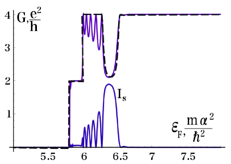
Figure 4: The dependence of normalized conductance and spin current on the Fermi energy. The upper and lower solid curves present $G(\varepsilon)$ and $I_{s}$ numerically calculated for $|p_{12}|=0.08m\alpha/\hbar$, $\Delta\varepsilon=0.32m\alpha^{2}/\hbar^{2}$, and $L=20\hbar^{2}/m\alpha$. The dashed curve shows $G(\varepsilon)$ calculated by means of Eq. (12).

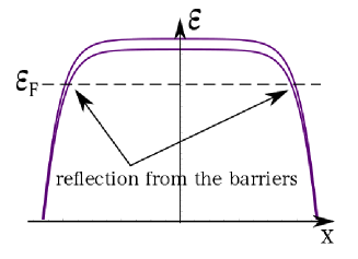
Figure 5: Spatial dependence of the gap in the spectrum. The lower curve shows the position of the maximum in the lower dispersion curve, and the upper curve shows the position of the minimum in the upper one. Electrons experience partial reflections at the points where the Fermi level crosses the gap in the spectrum.

Figure 4 shows the calculated electric conductance and spin current for $|p_{12}|=0.08m\alpha/\hbar$, $\Delta\varepsilon=0.32m\alpha^{2}/\hbar^{2}$, and $L=20\hbar^{2}/m\alpha$.estimate Solid lines show the values obtained by a numerical solution of Eqs. (8) with account taken of spatial variations of $\varepsilon_{1,2}$ and $\alpha$, and the dashed line shows analytical results calculated by means of Eq. (12). Both the numerically calculated conductance and spin current exhibit an oscillatory behavior as the Fermi level approaches the spectrum gap from below. This behavior is explained by quantum interference effects that arise due to the reflections of electrons from the ceiling of the allowed band at the edges of the wire where it goes down (see Fig. 5). The amplitude of the oscillations increases as the gap is approached because the reflection amplitude increases.

IV Conclusion

We have shown that Rashba spin-orbit interaction may open additional gaps in the spectrum of a multichannel quantum wire if the transverse confining potential is chosen appropriately. This happens if the energy levels of transverse quantization come in pairs and the matrix elements of transverse momentum between the corresponding states is sufficiently small. In this case, the conductance of the wire exhibits a dip and the spin current exhibits a spike inside the gap. If the contact is sufficiently long, the conductance in the dip drops from $4e^{2}/h$ to $2e^{2}/h$ and the current is fully spin-polarized in the transverse in-plane direction. This effect may be used for designing an all-electrical spin transistor. By applying a negative voltage to the middle longitudinal gate, one may increase the degree of spin polarization of the current from zero to 100% if the Fermi level is adjusted appropriately.

One of the main advantages of using electric bias for spin control is the ability to make it time-dependent. This can lead to non-trivial effects in the transport.Sadreev13 In the future, it would be of interest to study the effects of time-periodic bias in our model.

- (1) I. Z̆utić, J. Fabian, and S. Das Sarma, Rev. Mod. Phys. 76, 323 (2004).
- (2) E. I. Rashba, Fiz. Tverd. Tela (Leningrad) 2, 1224 (1960) [Sov. Phys. Solid State 2, 1109 (1960)].
- (3) J. Nitta, T. Akazaki, H. Takayanagi, and T. Enoki, Phys. Rev. Lett. 78, 1335 (1997).
- (4) G. Engels, J. Lange, Th. Schäpers, and H. Lüth, Phys. Rev. B 55, R1958 (1997).
- (5) L. S. Levitov and E. I. Rashba, Phys. Rev. B 67 115324 (2003).
- (6) S. Datta and B. Das, Appl. Phys. Lett. 56, 665 (1990).
- (7) H. C. Koo, J. H. Kwon, J. Eom, J. Chang, S. H. Han, and M. Johnson, Science 325, 1515 (2009).
- (8) Y. V. Pershin, J. A. Nesteroff, and V. Privman, Phys. Rev. B 69, 121306 (2004).
- (9) C. H. L. Quay, T. L. Hughes, J. A. Sulpizio, L. N. Pfeiffer, K. W. Baldwin, K. W. West, D. Goldhaber-Gordon and R. de Picciotto, Nature Physics 6, 336 (2010).
- (10) M. Governale and U. Zülicke, Phys. Rev. B 66,073311 (2002); Solid State Commun. 131, 581 (2004).
- (11) M. Eto, T. Hayashi, and Y. Kurotani, J. Phys. Soc. Jpn. 74, 1934 (2005).
- (12) F. Zhai and H. Q. Xu, Phys. Rev. B 76, 035306 (2007).
- (13) J.-F. Liu, Zh.-Ch. Zhong, L. Chen, D. Li, Ch. Zhang, and Zh. Ma, Phys. Rev. B 76, 195304 (2007).
- (14) F. Zhai, K. Chang, and H. Q. Xu, Appl. Phys. Lett. 92, 102111 (2008).
- (15) V. A. Sablikov, Phys. Rev. B 82, 115301 (2010).
- (16) D. Sánchez and L. Serra, Phys. Rev. B 74, 153313 (2006).
- (17) M. M. Gelabert, L. Serra, D. Sánchez, and R. López, Phys. Rev. B 81, 165317 (2010).
- (18) P. G. Silvestrov and E. G. Mishchenko, Phys. Rev. B 74, 165301 (2006).
- (19) The existence of maxima in the dispersion curves was predicted by A. V. Moroz and C. H. W. Barnes, Phys. Rev. B 60, 14272 (1999). However subsequent papers of other authorsGovernale02 found no maxima in them.
- (20) M. Büttiker, Y. Imry, R. Landauer, and S. Pinhas, Phys. Rev. B 31, 6207 (1985).
- (21) F. Zhai and H. Q. Xu, Phys. Rev. Lett. 94, 246601 (2005).
- (22) L.D. Landau, E.M. Lifshitz Mechanics. Vol. 1 (3rd ed.). Butterworth-Heinemann (1976).
- (23) This corresponds to nm in AlGaAs/GaAs heterostructures with eVcm and to nm in InAs quantum wells with eVcm.
- (24) Almas F. Sadreev and E. Ya. Sherman, Phys. Rev. B 88, 115302 (2013).