Critical behaviour in the QCD Anderson transition

Abstract:

We study the Anderson-type localisation-delocalisation transition found previously in the QCD Dirac spectrum at high temperature. Using high statistics QCD simulations with $N_{f}=2+1$ flavours of staggered quarks, we discuss how the change in the spectral statistics depends on the volume, the temperature and the lattice spacing, and we speculate on the possible universality of the transition from Poisson to Wigner-Dyson in the spectral statistics. Moreover, we show that the transition is a genuine phase transition: at the mobility edge, separating localised and delocalised modes, quantities characterising the spectral statistics become non-analytic in the thermodynamic limit. Using finite size scaling we also determine the critical exponent of the correlation length, and we speculate on possible extensions of the universality of Anderson transitions.

1 Introduction

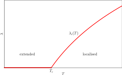
Figure 1: Schematic phase diagram of the 3D Anderson model (left) and QCD (right) in the disorder/eigenvalue plane.

It is well known that the properties of the low-lying modes of the Dirac operator are intimately related to the behaviour of QCD under chiral symmetry transformations, as clearly exemplified by the Banks-Casher relation [1]. In particular, it has been realised in recent years that their localisation properties change completely across the chiral transition/crossover. While below the critical temperature $T_{c}$ all the eigenmodes are delocalised, it has been shown [2, 3, 4, 5] that above $T_{c}$ the low-lying ones, up to some critical point $\lambda_{c}$, become localised; modes above $\lambda_{c}$ remain delocalised. Initially the evidence for this was mainly obtained in the quenched approximation and/or for the $SU(2)$ gauge group, but recently this scenario has been demonstrated in full QCD [5], by studying the spectrum of the staggered Dirac operator in numerical simulations of lattice QCD with $N_{f}=2+1$ flavours of quarks at physical masses [6]. An improved study, with much higher statistics and larger lattice volumes, has been presented at this conference [7].

The presence of a transition from localised to delocalised modes in the spectrum, as the one found in QCD above $T_{c}$, is a well known phenomenon in condensed matter physics, and it represents the main feature of the celebrated Anderson model [8] in three dimensions. The Anderson model aims at a description of electrons in a “dirty” conductor, by mimicking the effect of impurities through random interactions. In its lattice version, the model is obtained by adding a random on-site potential to the usual tight-binding Hamiltonian,

$$H=\sum_{n}\varepsilon_{n}|n\rangle\langle n|+\sum_{n}\sum_{\mu=1}^{3}|n+\hat{\mu}\rangle\langle n|+|n\rangle\langle n+\hat{\mu}|\,,$$ (1)

where $|n\rangle$ denotes a state localised on the lattice site $n$, and $\varepsilon_{n}$ are random variables drawn from some distribution, whose width $W$ measures the amount of disorder, i.e., of impurities in the system. The phase diagram of this model is sketched in Fig. 1. While for $W=0$ all the eigenmodes are delocalised, localised modes appear at the band edge as soon as the random interaction is switched on. The critical energy $E_{c}$ separating localised and delocalised modes is called “mobility edge”, and its value depends on the amount of disorder, $E_{c}=E_{c}(W)$. As $W$ increases, $E_{c}$ moves towards the center of the band, and above a critical disorder $W_{c}$ all the modes become localised. From the physical point of view, this signals a transition of the system from metal to insulator.

In Fig. 1 we also sketch a schematic phase diagram for QCD. Here the role of disorder is played by the temperature, while the energy is replaced by the eigenvalue of the Dirac operator. Localised modes are present in the low end of the spectrum above $T_{c}$, up to the “mobility edge” $\lambda_{c}(T)$. Around the critical temperature $\lambda_{c}$ vanishes [5], and below $T_{c}$ all the modes are extended.

In both models, localised modes appear where the spectral density is small. One then expects that they are not easily mixed by the fluctuations of the random interaction, which in turn suggests that the corresponding eigenvalues are statistically independent, obeying Poisson statistics. On the other hand, eigenmodes remain extended in the region of large spectral density also in the presence of disorder, and so one expects them to be basically freely mixed by fluctuations. The corresponding eigenvalues are then expected to obey the Wigner-Dyson statistics of Random Matrix Theory (RMT). This connection between localisation of eigenmodes and eigenvalue statistics provides a convenient way to detect the localisation/delocalisation transition and study its critical properties.

The transition from Poisson to RMT behaviour in the local spectral statistics is most simply studied by means of the so-called unfolded level spacing distribution (ULSD). Unfolding consists essentially in a local rescaling of the eigenvalues to have unit spectral density throughout the spectrum. The ULSD gives the probability distribution of the difference between two consecutive eigenvalues of the Dirac operator normalised by the local average level spacing. The ULSD is known analytically for both kinds of behaviour: in the case of Poisson statistics it is a simple exponential, while in the case of RMT statistics it is very precisely approximated by the so-called “Wigner surmise” for the appropriate symmetry class, which for QCD is the unitary class,

$$P_{\rm Poisson}(s)=e^{-s}\,,\qquad P_{\rm RMT}(s)=\frac{32}{\pi^{2}}s^{2}e^{-\frac{4}{\pi}s^{2}}\,.$$ (2)

Rather than using the full distribution to characterise the local spectral statistics, it is more practical to consider a single parameter of the ULSD. Any such quantity, having different values for Poisson and RMT statistics, can be used to detect the Poisson/RMT transition. In our study, we used the integrated ULSD and the second moment of the ULSD,

$$I_{\lambda}=\int_{0}^{s_{0}}ds\,P_{\lambda}(s)\,,\quad s_{0}\simeq 0.508\,,\qquad\langle s^{2}\rangle_{\lambda}=\int_{0}^{\infty}ds\,P_{\lambda}(s)\,s^{2}\,,$$ (3)

defined locally in the spectrum. The choice of $s_{0}$ was made in order to maximise the difference between the Poisson and RMT predictions, namely $I_{\rm Poisson}\simeq 0.398$ and $I_{\rm RMT}\simeq 0.117$; as for the second moment, the predictions are $\langle s^{2}\rangle_{\rm Poisson}=2$ and $\langle s^{2}\rangle_{\rm RMT}=3\pi/8$.

2 Numerical results

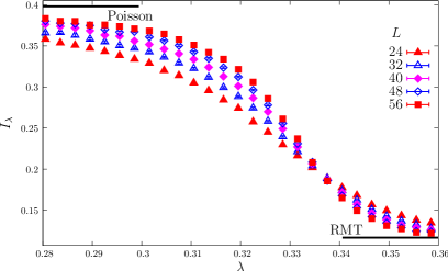
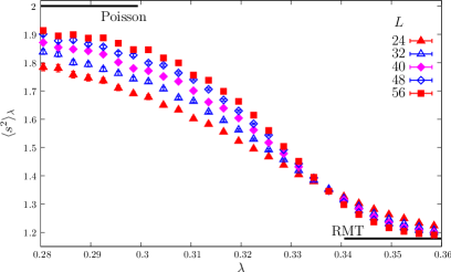
Figure 2: Integrated ULSD (left) and second moment of the ULSD (right), computed locally along the spectrum, for several lattice sizes. Here $\Delta\lambda=3\cdot 10^{-3}$.

The results presented here are based on simulations of lattice QCD using a Symanzik-improved gauge action and $2+1$ flavours of stout smeared staggered fermions, with quark masses at physical values [6]. We used a lattice of fixed temporal extension $N_{t}=4$ at $\beta=3.75$, corresponding to lattice spacing $a=0.125~{}{\rm fm}$ and physical temperature $T=394~{}{\rm MeV}\simeq 2.6T_{c}$. For different choices of spatial size $L=24,28,32,36,40,44,48,56$ in lattice units, we collected large statistics for eigenvalues and eigenvectors of the staggered Dirac operator in the relevant spectral range - see Ref. [7] for more details. Here and in the following the eigenvalues $\lambda$ are expressed in lattice units. Unfolding was done by ordering all the eigenvalues obtained on all the configurations (for a given volume) according to their magnitude, and replacing them by their rank order divided by the total number of configurations. We then computed locally the integrated ULSD and the second moment of the ULSD, by dividing the spectrum in small bins of size $\Delta\lambda$, computing the observables in each bin, and assigning the resulting value to the average value of $\lambda$ in each bin. We used several values for $\Delta\lambda$, ranging from $1\cdot 10^{-3}$ to $6\cdot 10^{-3}$.

In Fig. 2 we show the integrated ULSD $I_{\lambda}$ and the second moment of the ULSD $\langle s^{2}\rangle_{\lambda}$, for several values of the spatial volume. A transition from Poisson to RMT is clearly visible, and moreover it gets sharper and sharper as the volume of the lattice is increased. This suggests that the transition becomes a true phase transition in the thermodynamic limit.

3 Finite size scaling

To check if the Poisson/RMT transition in the spectral statistics (i.e., the localisation/delocalisation transition) is a genuine, Anderson-type phase transition, we have performed a finite size scaling analysis, along the lines of Refs. [11, 12, 13]. The Anderson transition is a second-order phase transition, with the characteristic length of the system $\xi_{\infty}$ diverging at the critical point $\lambda_{c}$ like $\xi_{\infty}(\lambda)\sim|\lambda-\lambda_{c}|^{-\nu}$. To determine the critical exponent $\nu$ and the critical point $\lambda_{c}$, one picks a dimensionless quantity $Q(\lambda,L)$, measuring some local statistical properties of the spectrum, and having different thermodynamic limits on the two sides of the transition (and possibly at the critical point), i.e.,

$$\lim_{L\to\infty}Q(\lambda,L)=\left\{\begin{aligned} &Q_{\rm Poisson}&&&&\lambda<\lambda_{c}&&&&\text{(localised)}\,,\\ &Q_{c}&&&&\lambda=\lambda_{c}&&&&\text{(critical)}\,,\\ &Q_{\rm RMT}&&&&\lambda>\lambda_{c}&&&&\text{(delocalised)}\,.\end{aligned}\right.$$ (4)

As the notation suggests, $Q(\lambda,L)$ is computed on a lattice of linear size $L$. For large enough volume, and close to the critical point, finite size scaling suggests that the dependence of $Q$ on $L$ is of the form $Q(\lambda,L)=f(L/\xi_{\infty}(\lambda))$. As $Q(\lambda,L)$ is analytic in $\lambda$ for any finite $L$, we must have

$$Q(\lambda,L)=F(L^{1/\nu}(\lambda-\lambda_{c}))\,,$$ (5)

with $F$ analytic. Here we have assumed that corrections to one-parameter scaling can be neglected.

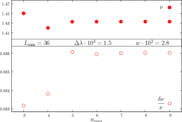
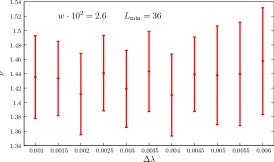
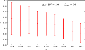
Figure 3: Dependence of the fitted value of $\nu$ and corresponding relative error as a function of the number of terms $n_{\rm max}$, in the case of $L_{\rm min}=36$, $\Delta\lambda\cdot 10^{3}=1.5$ and $w\cdot 10^{2}=2.8$ (left). Dependence of the fitted value of $\nu$ on the bin size $\Delta\lambda$ for the smallest fitting range (center) and on the width $w$ of the fitting range for the smallest bin size (right). Here $L_{\rm min}=36$.

If one determines $\lambda_{c}$ and $\nu$ correctly, the numerical data for $Q(\lambda,L)$ obtained for different lattice sizes should collapse on a single curve, when plotted against the scaling variable $L^{1/\nu}(\lambda-\lambda_{c})$. We then proceeded as follows: expanding the scaling function $F$ in powers of $\lambda-\lambda_{c}$, one gets

$$Q(\lambda,L)=\sum_{n=0}^{\infty}F_{n}\,L^{n/\nu}(\lambda-\lambda_{c})^{n}\,.$$ (6)

By truncating the series to some $n_{\rm max}$ and performing a fit to the numerical data, using several volumes at a time, one can then determine $\nu$ and $\lambda_{c}$, together with the first few coefficients $F_{n}$. For our purposes, the best quantity turned out to be the integrated ULSD $I_{\lambda}$. Our fitter was based on the MINUIT library [9]. Statistical errors were determined by means of a jackknife analysis. To check for finite size effects, we repeated the fit using only data from lattices of size $L\geq L_{\rm min}$ for increasing $L_{\rm min}$.

Systematic effects due to the truncation of the series for the scaling function, Eq. (6), are controlled by including more and more terms in the series, and checking how the results change. In order to circumvent the numerical instability of polynomial fits of large order, we resorted to the technique of constrained fits [10]. The basic idea of constrained fits is to use the available information to constrain the values of the fitting parameters. In our case, they are needed only to avoid that the polynomial coefficients of higher order take unphysical values. One then checks the convergence of the resulting parameters and of the corresponding errors as the number of terms is increased. After convergence, the resulting errors include both statistical effects and systematic effects due to truncation [10].

To set the constraints, we shift and rescale $F$ as follows, $\tilde{F}(x)=(F(x)-F_{\rm RMT})/(F_{\rm Poisson}-F_{\rm RMT})$, so that $\tilde{F}$ interpolates between 1 (localised/Poisson region) and 0 (delocalised/RMT region). The data indicate that $\tilde{F}$ changes rapidly, monotonically and almost linearly between 1 and 0 over a range $\delta x$. Any reasonable definition of $\delta x$ has then to satisfy $1+\tilde{F}_{1}\delta x\simeq 0$. Moreover, $\delta x$ provides a reasonable estimate of the radius of convergence $\rho$ of the series. Furthermore, it is known that $(\tilde{F}_{n+1}/\tilde{F}_{n})\rho\to 1$ as $n\to\infty$, and so we expect $\tilde{F}_{n}\rho^{n}\sim 1$ (at least for large $n$). One then finds that $\tilde{F}_{n}/(-\tilde{F}_{1})^{n}$ is expected to be of order 1. This constraint was imposed rather loosely, by asking $\tilde{F}_{n}/(-\tilde{F}_{1})^{n}$ to be distributed according to a Gaussian of zero mean and width $\sigma=10$ for $n\geq 4$. We did not impose any constraint on the coefficients $F_{n}$ with $n<4$, as well as on $\nu$ and $\lambda_{c}$. The results of the constrained fits converge rather rapidly as $n_{\rm max}$ is increased, see Fig. 3. We went as far as $n_{\rm max}=9$, and we used the corresponding results for the following analyses.

The effects of the choice of bin size and fitting range were checked by varying the bin size $\Delta\lambda$ and the width $w$ of the fitting range, which was centered approximately at the critical point. The results show a slight tendency of $\nu$ to decrease as $\Delta\lambda$ is decreased, but it is rather stable for $\Delta\lambda\cdot 10^{3}\lesssim 3$. There is also a slight tendency of $\nu$ to increase as $w$ is decreased, becoming rather stable for $w\cdot 10^{2}\lesssim 3$. See Fig. 3. To quote a single value for $\nu$, we averaged the central values obtained for $1\leq\Delta\lambda\cdot 10^{3}\leq 3$ and $2.6\leq w\cdot 10^{2}\leq 3$. As the error is also rather stable within these ranges, we quote its average as the final error on $\nu$ for each choice of $L_{\rm min}$. We have checked that other prescriptions (e.g., extrapolating to vanishing $w$ and/or $\Delta\lambda$, or changing – within reasonable bounds – the ranges of $w$ and $\Delta\lambda$ over which the final average is performed) give consistent results within the errors.

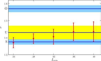
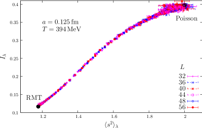
Figure 4: Dependence of the fitted value of $\nu$, averaged over $2.6\leq w\cdot 10^{2}\leq 3.0$ and $1.0\leq\Delta\lambda\cdot 10^{3}\leq 3.0$, on $L_{\rm min}$. The values of $\nu$ obtained in the three symmetry classes of the 3D Anderson model (symplectic, $\nu_{\rm S}=1.375(16)$ [16], unitary $\nu_{\rm U}=1.43(4)$ [14] and orthogonal $\nu_{\rm O}=1.57(2)$ [15]) are shown for comparison together with their errors (left). Plot of $I_{\lambda}$ against $\langle s^{2}\rangle_{\lambda}$ for several lattice sizes (right).

Concerning finite size effects, the fitted value of $\nu$ increases with $L_{\rm min}$, stabilising around $L_{\rm min}=36$, see Fig. 4. This signals that our smallest volumes are still too small for one-parameter scaling to work, and that finite size corrections are still important there. On the other hand, as the difference between the values obtained with $L_{\rm min}=36$ and $L_{\rm min}=40$ is much smaller than the statistical error, one-parameter scaling works fine for our largest volumes.

The value for the critical point $\lambda_{c}\simeq 0.336$ was obtained through the same procedure described above. As a function of $L_{\rm min}$, the fitted value of $\lambda_{c}$ shows no systematic dependence, and different choices of $L_{\rm min}$ give consistent values within the errors.

Our result for the critical exponent $\nu=1.43(6)$ is compatible with the result obtained for the three-dimensional unitary Anderson model $\nu_{\rm U}=1.43(4)$ [14]. This strongly suggests that the transition found in the spectrum of the Dirac operator above $T_{c}$ is a true Anderson-type phase transition, belonging to the same universality class of the three-dimensional unitary Anderson model.

4 Shape analysis

From the point of view of random matrix models, Fig. 2 shows that the local spectral statistics along the spectrum are described by one-parameter families of models, with spectral statistics interpolating between Poisson and Wigner-Dyson along some path in the space of probability distributions. To check if the appropriate one-parameter family depends on the size of the lattice, one can simply plot a couple of parameters of the ULSD against each other (thus projecting the path onto a two-dimensional plane in the space of probability distributions): if points are seen to collapse on a single curve, irrespectively of $L$, then the intermediate ULSDs lie on a universal path in the space of probability distributions [17].

In Fig. 4 we show $I_{\lambda}$ and $\langle s^{2}\rangle_{\lambda}$ plotted against each other for several volumes, and we see that they indeed lie on a single curve. As $L$ is increased, points corresponding to a given value of $\lambda$ flow towards the Poisson or RMT “fixed points”, while flowing away from an unstable fixed point corresponding to $\lambda_{c}$, where a different universality class for the spectral statistics is expected. Similar plots made by changing $T$ and/or $a$ are compatible with a similar universality of the path, but statistical errors are still too large to reach a definitive conclusion.

The transition from Poisson to Wigner-Dyson behaviour in finite volume is therefore expected to be described by a universal one-parameter family of random matrix models [18]. Comparing with analogous results for the Anderson model, it turns out that the spectral statistics at the critical point in the two models are compatible [18].

References

- [1] T. Banks and A. Casher, Nucl. Phys. B 169 103 (1980).
- [2] A.M. García-García and J.C. Osborn, Phys. Rev. D 75 034503 (2007) [hep-lat/0611019].
- [3] T.G. Kovács, Phys. Rev. Lett. 104 031601 (2010) [arXiv:0906.5373 [hep-lat]].
- [4] T.G. Kovács and F. Pittler, Phys. Rev. Lett. 105 192001 (2010) [arXiv:1006.1205 [hep-lat]].
- [5] T.G. Kovács and F. Pittler, Phys. Rev. D 86 114515 (2012) [arXiv:1208.3475 [hep-lat]].
- [6] Y. Aoki, Z. Fodor, S. D. Katz and K. K. Szabó, JHEP 0601, 089 (2006) [hep-lat/0510084]; S. Borsányi, G. Endrődi, Z. Fodor, A. Jakovác, S. D. Katz, S. Krieg, C. Ratti and K. K. Szabó, JHEP 1011, 077 (2010) [arXiv:1007.2580 [hep-lat]].
- [7] M. Giordano, T.G. Kovács and F. Pittler, PoS LATTICE 2013 212 (2013) [arXiv:1311.1770 [hep-lat]].
- [8] P.W. Anderson, Phys. Rev. 109 1492 (1958).
- [9] F. James and M. Roos, Comput. Phys. Commun. 10 343 (1975).
- [10] G. P. Lepage, B. Clark, C. T. H. Davies, K. Hornbostel, P. B. Mackenzie, C. Morningstar and H. Trottier, Nucl. Phys. Proc. Suppl. 106 12 (2002) [hep-lat/0110175].
- [11] E. Hofstetter and M. Schreiber, Phys. Rev. B 49 14726 (1994).
- [12] B.I. Shklovskii, B. Shapiro, B.R. Sears, P. Lambrianides and H.B. Shore, Phys. Rev. B 47 11487 (1993).
- [13] F. Siringo and G. Piccitto, J. Phys. A 31 5981 (1998).
- [14] K. Slevin and T. Ohtsuki, Phys. Rev. Lett. 78 4083 (1997). [cond-mat/9704192 [cond-mat.dis-nn]].
- [15] K. Slevin and T. Ohtsuki, Phys. Rev. Lett. 82 382 (1999) [cond-mat/9812065 [cond-mat.dis-nn]].
- [16] Y. Asada, K. Slevin and T. Ohtsuki, J. Phys. Soc. Jpn. 74 supplement 238 (2005) [cond-mat/0410190 [cond-mat.dis-nn]].
- [17] I. Varga, E. Hofstetter, M. Schreiber and J. Pipek, Phys. Rev. B 52 7783 (1995) [cond-mat/9407058] .
- [18] S.M. Nishigaki, M. Giordano, T.G. Kovács and F. Pittler, PoS LATTICE 2013, 018 (2013).