On the role of the chaotic velocity in relativistic kinetic theory

Abstract

In this paper we revisit the concept of chaotic velocity within the context of relativistic kinetic theory. Its importance as the key ingredient which allows to clearly distinguish convective and dissipative effects is discussed to some detail. Also, by addressing the case of the two component mixture, the relevance of the barycentric comoving frame is established and thus the convenience for the introduction of peculiar velocities for each species. The fact that the decomposition of molecular velocity in systematic and peculiar components does not alter the covariance of the theory is emphasized. Moreover, we show that within an equivalent decomposition into space-like and time-like tensors, based on a generalization of the relative velocity concept, the Lorentz factor for the chaotic velocity can be expressed explicitly as an invariant quantity. This idea, based on Ellis’ theorem, allows to foresee a natural generalization to the general relativistic case.

1 Introduction

The concept of chaotic velocity was introduced in non-relativistic kinetic theory since its early developments Brush (1, 2). Its importance in the formulation of the theory, as well as its connection with the corresponding phenomenology, resides in the fact that it allows to separate mechanic and thermodynamic effects. Moreover, the heat flux was defined by Clausius Brush (1) as the flow of energy arising from the purely chaotic component of the motion. Eventhough the chaotic velocity is a standard tool in the non relativistic formalism, it has been mostly ignored in the relativistic case. The first work recognizing its value and the need to include it in the relativistic formulation in order to clearly define dissipative fluxes was written by Sandoval and García-Colín Sandoval physica A 2000 (3). In that work, Lorentz transformations were introduced with the purpose of extracting the peculiar component from the molecular velocity. Such idea was carried further in several publications, in particular Ref. Garcia Perciante 2012 (4) formulates a covariant kinetic theory in terms of hydrodynamic and chaotic velocities in the framework of special relativity. Also, Ref. Garcia-Perciante Chaotic Velocity (5) includes a somehow thorough discussion and conceptual explanation of such a decomposition.
In this work we review the arguments presented in the references cited above and provide with two additional contributions. First, we explicitly show how the introduction of Lorentz transformations and the use of the Lorentz factor $\gamma$ for one particle evaluated in the comoving frame of the fluid as the key variable, preserve the covariance of the theory. The use of such factor allows to express all variables and fluxes in a similar way to the non-relativistic case. The particular case of a binary mixture is addressed, in which the chaotic velocity of the species plays a critical role as well as the system moving with the barycentric velocity. Secondly, we show how by introducing the concept of relative velocity, proposed in a different context by Ellis ellis articulo (6, 7), one is able to split the hydrodynamic velocity into two components in such a way that the space-like part permits the expression of the $\gamma$ factor in a covariant way for a general metric.
The structure of this paper is as follows. In the second section we make a brief review of what is the meaning and implications of the use of the chaotic velocity in non-relativistic kinetic theory. The third section addresses the introduction of the chaotic velocity in special relativity and discusses the case of the binary mixture. The decomposition in terms of a space-like relative velocity is introduced in the fourth section as a suitable alternative for extending the concept to the framework of general relativity. The last section includes concluding remarks and perspectives.

2 The chaotic velocity in non-relativistic kinetic theory

As mentioned above, the importance of chaotic velocity, also known as peculiar or thermal velocity, in non relativistic kinetic theory is due to the fact that it allows one to separate diffusive and convective effects. The relevance of this property can be appreciated by considering for example the heat flux, which is the energy flux due to the molecular nature of matter. By introducing such concept when analyzing energy transport, mechanical contributions arising from the motion of the system as a whole become separated from those related to thermal agitation.

To illustrate the point we review the discussion in Ref. Garcia Perciante 2012 (4) and Chapman (8) by starting with the non relativistic Boltzmann equation for a simple gas in the absence of external forces, this is

$$\frac{\partial f}{\partial t}+\vec{v}\cdot\nabla f=J\left(ff^{\prime}\right).$$ (1)

Here $f=f\left(\vec{r},\vec{v},t\right)$ is the distribution function per particle, $\vec{v}$ is the velocity of one particle with mass $m$, as measured by an observer in the laboratory frame. The term on the right hand side accounts for the variations in the distribution function due to particle collisions. From Eq. (1) one can obtain the balance equations by using the standard method, that is, by multiplying it by the collisional invariants, namely the mass, momentum and energy, and then integrating over velocity space Chapman (8). This process leads to the definitions, with the help of the local equilibrium assumption, of the thermodynamic local variables as well as the corresponding fluxes as averages over the distribution function. For these definitions to be in accordance with the phenomenology and the physical interpretation of such quantities, it is crucial to introduce the decomposition

$$\vec{v}=\vec{c}+\vec{u},$$ (2)

where $\vec{u}$ and $\vec{c}$ are the hydrodynamic and chaotic velocities respectively. The procedure is standard and leads to the following definitions for the state variables particle density, hydrodynamic velocity and internal energy

$$n\left(\vec{r},t\right)=\int fd\vec{v},$$ (3)

$$\vec{u}\left(\vec{r},t\right)=\frac{1}{n}\int\vec{v}fd\vec{v},$$ (4)

and

$$ne\left(\vec{r},t\right)=\frac{1}{2}m\int c^{2}fd\vec{c},$$ (5)

respectively. Notice how the internal energy arises solely from the chaotic component of the velocity. The total energy is given by

$$\frac{1}{2}m\int v^{2}fd\vec{c}=\frac{1}{2}mnu^{2}+ne,$$ (6)

where Eq. (2) has been introduced for $\vec{v}$ and use has been made of the fact that, in view of Eq. (4), $\int\vec{c}fd\vec{c}=0$. Regarding the fluxes one has, firstly for the stress tensor

$$\overleftrightarrow{\tau}\left(\vec{r},t\right)=m\int\vec{v}\vec{v}fd\vec{c}=m\int\vec{c}\vec{c}fd\vec{c}+\rho\vec{u}\vec{u},$$ (7)

where $\rho=mn$. Note that the first term on the right hand side of Eq. (7) refers strictly to the chaotic velocity $\vec{c}$ and not the molecular one $\vec{v}$. From this term, both the hydrostatic pressure part as well as the one related with viscous dissipation will arise. Due to the use of Eq. (2) the contribution of the hydrodynamic velocity $\vec{u}$ to the stress tensor is driven to the convective term $\rho\vec{u}\vec{u}$. Secondly, from the energy balance equation, which is given by

$$\rho\frac{de}{dt}+\nabla\cdot\vec{J}_{q}+\left(\overleftrightarrow{\tau}^{k}\right):\nabla\vec{u}=0,$$ (8)

one identifies the heat flux

$$\vec{J}_{q}\left(\vec{r},t\right)=\frac{1}{2}m\int c^{2}\vec{c}fd\vec{c},$$ (9)

and the tensor associated with the viscosity

$$\overleftrightarrow{\tau}^{k}\left(\vec{r},t\right)=m\int\vec{c}\vec{c}fd\vec{v},$$ (10)

which appear as dissipative fluxes in such an equation. We know from thermostatics that the internal energy is defined with no contributions from the motion of the system as a whole. Equation (8) is clearly consistent with this, since in it internal energy is dissipated only by the heat flux $\vec{J}_{q}$ and the viscous contribution $\overleftrightarrow{\tau}^{k}$ which only depend on the chaotic velocity.

Having reviewed these definitions, it is clear that the decomposition given by Eq. (2) is crucial for the physical interpretation of the different contributions to fluxes and thermodynamic variables. Notice that the separation of chaotic and hydrodynamic velocities within the molecular one can also be interpreted as a change of reference frame. This idea permits the extension to the framework of special relativity which will be the focus of the next section. This interpretation is discussed in Ref. Garcia-Perciante Chaotic Velocity (5) for the simple fluid, we repeat the argument here in order to generalize it to the fluid mixture.

For the simple fluid, the molecular velocity $\vec{v}$ is the velocity of the molecule as measured in a laboratory frame while the hydrodynamic velocity $\vec{u}$ is the field of velocities that defines the motion of the fluid with respect to it. The chaotic velocity $\vec{c}$ is thus clearly the velocity of the particles measured in a comoving frame which is at rest with respect to the fluid element. In other words, an observer in a locality on this comoving frame will observe the fluid at rest in average and only measure the peculiar velocity of the molecules. These ideas are illustrated in Fig. 1 where $\bar{S}$ is the comoving frame, in which an observer will measure as the molecular velocity of some particle only the chaotic component $\vec{c}$. On the other hand an observer in the $S$ frame will measure for the same particle its corresponding Galilean transformed velocity, i.e. $\vec{v}=\vec{c}+\vec{u}$.

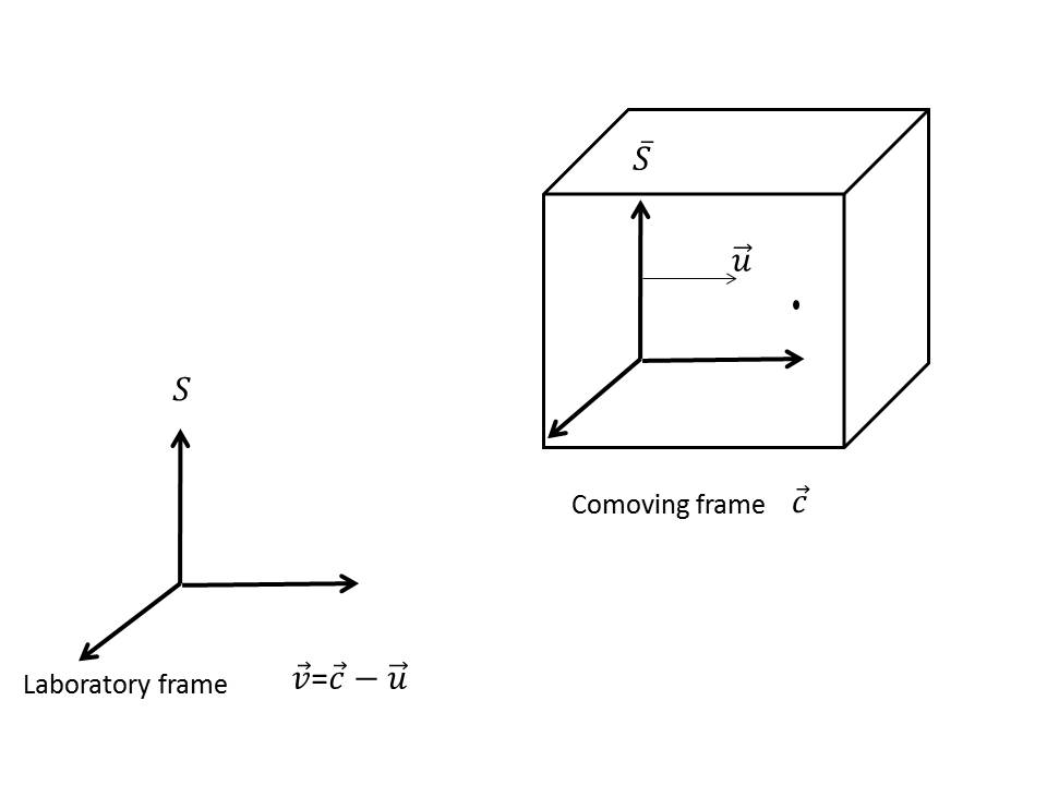
Figure 1: Comoving frame $\bar{S}$ moving with velocity $\vec{u}$ respect to the laboratory frame $S$. The chaotic velocity is $\vec{c}$.

An observer in the $S$ frame will obtain in his measurements not only the dissipative effects driven from the molecular nature of the fluid but also those convective contributions that arise form the motion of the fluid as one big mechanical object. On the other hand, one observer in the comoving frame will only measure the thermal effects. This frame is convenient when we are interested in the evaluation of thermodynamic properties because it leads in a very natural way to the conceptualization of thermodynamics from the kinetic theory point of view.

For the case of mixtures, the concept of chaotic velocity has another feature which underlines its importance. In such a case, the definition is given by

$$\vec{c}_{i}=\vec{v}_{i}-\vec{u}.$$ (11)

Here the subindex $i$ denotes the velocity for the $i$-th species in the gas ($i=\left\{1,...,M\right\}$) with $M$ constituents and $\vec{u}\left(\vec{r},t\right)$ is the barycentric velocity of the gas defined by

$$n\vec{u}=\sum_{i=1}^{M}n_{i}\vec{u}_{i},$$ (12)

being $n_{i}\left(\vec{r},t\right)=\int f_{i}d\vec{v}_{i}$ and $\vec{u}_{i}\left(\vec{r},t\right)=\frac{1}{n_{i}}\int\vec{v}_{i}f_{i}d\vec{v}_{i}$ the density and the hydrodynamic velocity for the species $i$ respectively. Here we have $\left\{n_{1},...,n_{M},\vec{u},e\right\}$ as local thermodynamic state variables. The distribution function per particle $f_{i}$ for the constituent $i$ is the solution of the Boltzmann equation for the species $i$. In the case of a mixture with $M$ components we have a set of $M$ Boltzmann equations, one per species, and all of them coupled by the collisional terms. The details of corresponding formalism can be found in Chapter 6 of Ref Ferziger (9).

In the case of mixtures, the chaotic velocity plays crucial role, not only because of the arguments discussed above, but also because it helps to establish the diffusion of one species into the other. The dissipative mass flux for the species $i$ is defined by

$$\vec{J}_{i}\left(\vec{r},t\right)=\frac{1}{n_{i}}\int\vec{c}_{i}fd\vec{c}_{i},$$ (13)

and the relation

$$\sum_{i}\vec{J}_{i}=\vec{0},$$ (14)

is a consequence of the definition (11). This last argument is what actually gives sense to the idea of diffusion in mixtures from the kinetic theory point of view. In the next section we will show how these ideas are incorporated into relativistic kinetic theory while preserving the covariance of the theory.

3 The chaotic velocity in special relativistic kinetic theory

Relativistic kinetic theory has been under development since 1911, when the first proposal for an equilibrium distribution function was presented JUTTNER (10). The theory underwent a slow but steady development and many relevant sources can be cited. The reader is referred to the classical textbooks in Refs. Groot-Leewen-Weert (11, 12) which abridge most of the work done in this direction. However, reviewing the literature one can conclude that the concept of chaotic velocity has been ignored up to this century. As mentioned above, this absence was first pointed out in Ref. Sandoval physica A 2000 (3) where Lorentz transformations where firstly introduced, a subsequent work rounded the idea Garcia Perciante 2012 (4) which is currently being applied with success in different frameworks (see for example Refs. Garcia-Perciante Mendez Heat conduction … revisited (13, 14, 15, 16)). In this section we show how the chaotic velocity is introduced in special relativistic kinetic theory by considering Lorentz transformations as a direct generalization of the Galilean ones used in the previous section both for the single component gas as well as for the mixture. Some details of this formalism can be found in Ref. Moratto Thesis (17).

Following a procedure analogous to the one described in the previous section, one starts form the relativistic Boltzmann equation, given by

$$v^{\alpha}f_{,\alpha}=J\left(ff^{\prime}\right).$$ (15)

Multiplying Eq. (15) by the collisional invariants and integrating over velocity space one obtains conservation equations for two fluxes, the particle flux and the energy momentum tensor are given by

$$N^{\mu}=\int v^{\mu}fdv^{*},$$ (16)

and

$$T^{\mu\nu}=\int v^{\mu}v^{\nu}fdv^{*},$$ (17)

respectively. Here $dv^{*}$ is the invariant volume element CERCIGNANI (12). At this point, the introduction of the chaotic velocity is desirable in order to distinguish, in a similar fashion as in the non-relativistic case, the different components in each of these tensors. The corresponding calculation together with a thorough discussion can be found in Ref. Garcia Perciante 2012 (4). Here we discuss in depth the transformation and the definition of the relevant variable as well as its invariance. Let $U^{\mu}$ be the hydrodynamic four-velocity of the gas defined by

$$U^{\mu}=\frac{dx^{\mu}}{d\tau},$$ (18)

where $x^{\mu}$ is the four-position of the volume element of the gas, as measured in a laboratory frame, and $\tau$ is the proper time. Thus, $U^{\mu}$ is the four velocity of the fluid with respect the laboratory inertial frame. The metric in this context is given by

$$ds^{2}=dx^{2}+dy^{2}+dz^{2}-c^{2}dt^{2},$$ (19)

in correspondence with Minkowski’s metric. The components of $U^{\mu}$ are thus

$$U^{\mu}=\gamma_{u}\left(\vec{u},c\right),$$ (20)

where $\gamma_{u}$ is the Lorentz factor, given by

$$\gamma_{u}=\frac{1}{\sqrt{1-\frac{u^{2}}{c^{2}}}},$$ (21)

with $u^{2}=\vec{u}\cdot\vec{u}$. We can also define another four-velocity, namely the four-velocity for one particle as observed in the laboratory frame

$$v^{\mu}=\gamma_{v}\left(\vec{v},c\right),$$ (22)

where clearly $\gamma_{v}=\left(1-v^{2}/c^{2}\right)^{-1/2}$ with $v^{2}=\vec{v}\cdot\vec{v}$. It is also important to underline that both four-velocities, $U^{\mu}$ and $v^{\mu}$ are time-like vectors, i.e.

$$U^{\mu}U_{\mu} < 0,$$ (23)

$$v^{\mu}v_{\mu} < 0,$$ (24)

and it is always possible to find a frame of reference in which the world line of any of these vectors has only a temporal component Moller (18). For example, for the vector $U^{\mu}$ it is always possible to find a frame of reference in which

$$U^{\mu}=\left[\vec{0},c\right].$$ (25)

Then, for every inertial frame the invariant constructed with the scalar contraction of the two four-velocities in question $U^{\mu}$ and $v^{\mu}$ reads

$$U^{\alpha}v_{\alpha}=\gamma_{u}\gamma_{v}\vec{u}\cdot\vec{v}-\gamma_{u}\gamma_{v}c^{2}.$$ (26)

In particular, if we choose the frame defined by equation (25), the invariant (26) reads

$$U^{\alpha}v_{\alpha}=-\gamma_{k}c^{2},$$ (27)

where $\gamma_{k}$ is the Lorentz factor evaluated with the velocity of the particle in such frame, whose magnitude we denote by $k$. This quantity is, by its definition given in Eq. (27), an invariant. Notice that this variable is also proportional to the particles’ kinetic energy measured in the comoving frame. Because of this, it will be present in the integrals for various thermodynamic quantities and it is thus worthwhile to point out that once evaluated in the comoving frame, this factor is a Lorentz invariant in a similar way as the rest mass and proper time are.

The frame defined by Eq. (25) is of great conceptual importance. In this framework it is identified as the comoving frame, in a similar way as was conceived in the non-relativistic case. Then, by following the discussion of the last section, through the consideration of variables and fluxes in this frame is how one can isolate the dissipative effects from the total quantities which also include the convective ones.

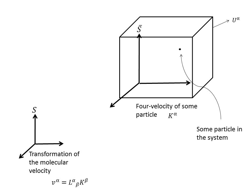
Figure 2: Comoving frame $\bar{S}$ moving with four-velocity $U^{\mu}$ respect to the laboratory frame $S$. The chaotic four-velocity is $K^{\alpha}$.

Figure 2 shows this frame in relation with the laboratory frame where

$$L_{\text{ }\beta}^{\alpha}=\frac{\partial\overline{x}^{\alpha}}{\partial x^{\beta}}$$ (28)

is a Lorentz boost to the frame $\bar{S}$. Also, we have introduced the particle four-velocity, as measured in the comoving frame $K^{\alpha}$, in order to have a distinct notation for the chaotic velocity as in the non-relativistic formalism. The relation between $K^{\alpha}$ and $v^{\alpha}$ is clearly given by

$$v^{\alpha}=L_{\text{ }\beta}^{\alpha}K^{\beta}.$$ (29)

Equation (29) plays the role of Eq. (2). With these definitions, one is able to write state variables and thermodynamic fluxes as averages over chaotic quantities. For example for the internal energy and heat flux one has

$$ne=mc^{2}\int\gamma_{k}^{2}fdK^{*},$$ (30)

and

$$q^{\beta}=mc^{2}L_{\beta}^{\mu}\int\gamma_{k}K^{\beta}fdK^{*}.$$ (31)

It is important to point out that these definitions are similar in structure as the ones in the non-relativistic case and highlight the physical nature of the corresponding quantities: the internal energy as the average of the chaotic kinetic energy and the heat flux as the flux of such quantity, measured in the comoving frame where mechanical effects are not present. Notice that the heat flux definition includes a Lorentz transformation. The deduction of these formulas can be found to detail in Ref. Garcia Perciante 2012 (4). What we want to point out here is the covariance of both quantities. Indeed, the internal energy is an invariant, it does not depend on the observer and is thus calculated in the comoving frame where it is the average of the kinetic energy of the particles. On the other hand, the heat flux is a tensor and thus transforms, in this case in a contravariant way. Indeed, Eq. (31) can be rewritten as $q^{\nu}=L_{\mu}^{\nu}Q^{\nu}$ where $Q^{\nu}$ is the heat flux as defined by Clausius Brush (1).

For the case of mixtures, the concept of chaotic velocity allows, as in the previous section, for a clear definition of the diffusive fluxes. As before, the comoving frame is replaced by the frame moving with the barycentric velocity and chaotic velocities for each species can be found by considering a Lorentz boost from the laboratory frame to it. The fact that the species have different averages for chaotic velocities gives rise, as before, to what we understand as diffusive fluxes. To clarify this idea we consider some definitions from the relativistic kinetic theory for mixtures Val-3 (16, 19). The particle four-flow is defined by

$$N_{(i)}^{\alpha}\equiv m_{(i)}\int v_{(i)}^{\alpha}f_{(i)}dv_{(i)}^{*}$$ (32)

for the $(i)$-th component of the gas, $m_{(i)}$ is the rest mass of some particle of the species $(i)$ and $f_{(i)}$ the corresponding solution of the Boltzmann equation. The total particle flow, that is, the flow with the contribution of the $M$ species will be

$$N^{\alpha}=\sum_{(i)=1}^{M}N_{(i)}^{\alpha}.$$ (33)

We can introduce the idea of chaotic velocity for the mixture in the following way

$$v_{(i)}^{\alpha}=L_{\beta}^{\alpha}K_{(i)}^{\beta},$$ (34)

where the Lorentz transformation $L_{\beta}^{\alpha}$ is constructed with the barycentric velocity $U^{\alpha}$ defined by

$$nU^{\alpha}=\sum_{(i)=1}^{M}n_{(i)}U_{(i)}^{\alpha}$$ (35)

with

$$n_{(i)}U_{(i)}^{\alpha}=\int v_{(i)}^{\alpha}f_{(i)}dv_{(i)}^{*}.$$ (36)

By introducing Eq. (34) in Eq. (32), we obtain a flow of particles evaluated in the comoving frame, which is the diffusion of one species into the fluid, since it does not involve convective effects. Thus, we have for the diffusive flux

$$J_{(i)}^{\mu}=m_{(i)}\int K_{(i)}^{\mu}f_{(i)}dK_{(i)}^{*}.$$ (37)

Equation (37) satisfies the relation

$$\sum_{(i)=1}^{M}J_{(i)}^{\mu}=\left(\vec{0},n\right),$$ (38)

where

$$n=\sum_{(i)}^{M}n_{(i)}.$$ (39)

We can see from Eqs. (37) and (38) that the diffusion has the same properties and physical meaning than in the non-relativistic case. This argument reinforces the importance of the use of chaotic velocity, Eq (34). These elements are valid only in special relativity, some ideas regarding the general relativistic generalization are explored in the next section.

4 The chaotic velocity in general coordinates

In this section, the kinetic energy introduced before will be expressed as an invariant representing the chaotic part of the particles’ energy for a general metric tensor, allowing for an extension to curved space-times. In order to accomplish this task, we recall a theorem given by G. Ellis which proposes one very particular relation between four-velocities in order to introduce a relative velocity in a covariant fashion ellis articulo (6, 7). Indeed, it is straightforward to show that given two time-like four-vectors $\left\{v^{\mu},U^{\mu}\right\}$, it is possible to find one space-like four-vector $S^{\mu}$ such that

$$v^{\mu}=\eta\left(U^{\mu}+S^{\mu}\right)$$ (40)

with

$$S^{\mu}U_{\mu}=0,$$ (41)

and

$$\eta=\frac{1}{\sqrt{1-\frac{S_{\nu}S^{\nu}}{c^{2}}}}.$$ (42)

For the sake of clarity, we recall that while a time-like four-vector has the properties described in the previous section, a space-like vector $S^{\mu}$ satisfies

$$S_{\nu}S^{\nu}>0,$$ (43)

and it is always possible to find a reference frame in which the temporal component of $S^{\mu}$ is zero, that is

$$S^{\mu}=\left[\vec{s},0\right].$$ (44)

This theorem is valid in general but in this case we associate $v^{\mu}$ with the molecular four-velocity and $U^{\mu}$ with the barycentric or hydrodynamic four-velocity, both being time-like since $v^{\mu}v_{\mu}=U^{\mu}U_{\mu}=-c^{2}$.

Equation (40) is valid in any frame and, since $U^{\mu}$ is time-like, it is possible to evaluate it where $U^{\mu}=\left[\vec{0},c\right]$ which is precisely the fluid’s comoving frame.

$$v_{\text{CM}}^{\alpha}=\eta\left(\left[\vec{0},c\right]+S_{\text{CM}}^{\alpha}\right),$$ (45)

Now, in the special relativistic case addressed in the previous section, the molecular velocity in the comoving frame is $K^{\alpha}$. Also, since $S^{\mu}$ is orthogonal to $U^{\mu}$ (Eq. (41)), in the comoving frame it only has temporal components such that we have

$$K^{\alpha}=\eta\left(\left[\vec{0},c\right]+\left[\vec{s},0\right]\right),$$ (46)

which, since $K^{\alpha}=\gamma_{k}\left[\vec{k},c\right]$ yields $\gamma_{k}=\eta$ and $\vec{s}=\vec{k}$. One concludes that in special relativity the $\gamma_{k}$ factor, which is proportional to the chaotic energy and is thus required as a variable in order to express thermodynamic quantities, can be written in general as

$$\gamma_{k}=\frac{1}{\sqrt{1-\frac{S_{\nu}S^{\nu}}{c^{2}}}},$$ (47)

where $S^{\mu}$ is given by Eq. (40) and is a space-like vector which in the comoving frame of the fluid, only has spatial components which coincide with the chaotic velocity ones. This reinforces the covariance of the calculations that have been worked in the literature Garcia Perciante 2012 (4, 13, 16, 19, 20) in the framework of special-relativistic kinetic theory. Also, and most importantly, this reasoning sheds light on a possible way to extend these ideas to the general relativistic case.

For a general metric tensor $g_{\mu\nu}$, the kinetic energy of the molecules measured in the comoving frame is given by $-mU^{\mu}v_{\mu}$. Introducing the general decomposition given in Eq. (40) one obtains

$$mU^{\mu}v_{\mu}=-m\gamma c^{2},$$ (48)

which leads to the interpretation of $\gamma=\eta$, given by Eq. (42), as the generalization of $\gamma_{k}$ for a general metric. This is a promising result since integrals representing state variables and thermodynamic fluxes may be expressed in terms of this decomposition having, in particular, the invariant $\gamma$ for energy quantities available.

5 Conclusions

In this paper we have revisited the concept of chaotic velocity in the framework of relativistic kinetic theory by firstly recalling some basic aspects of the non-relativistic case where such idea was included since its early developments. Then, we addressed the special relativistic case, emphasizing both its importance in the mixture case as well as the covariance of the theory based on the invariance of the relevant variable $\gamma_{k}$, representing the energy of the particles in the comoving frame. In such a frame, in which the hydrodynamic or barycentric velocity vanishes, the dissipative effects are isolated since mechanical effects are not present.

The importance of the chaotic velocity in the mixture case resides in the fact that the state variable in such a case is the barycentric velocity (not the hydrodynamic velocity for each species) and thus, the diffusive fluxes of the species are relative to a frame comoving with it. These fluxes are identified in this framework as the average of the momentum of the particles measured in this comoving frame and the sum of them vanishes in it.

Regarding the covariance of the formalism, we provided with two solid arguments. Firstly, what is a decomposition of velocities in the non-relativistic case, is viewed as a reference frame transformation for the special relativistic case. Such transformation consists in a Lorentz boost which preserves the covariance. The relevant variable for the calculation of fluxes and variables turns out to be proportional to the chaotic component of the particles’ energy which is expressed through an already evaluated Lorentz factor $\gamma$. The second argument relies on Ellis’ theorem which introduces a space-like relative velocity. We showed how $\gamma_{k}$ can be expressed in terms of the magnitude of such a tensor. This idea yields an invariant expression for this important quantity which can be generalized for a general metric.

We conclude that the chaotic velocity is a valuable concept and can be introduced in relativistic kinetic theory in a covariant fashion which allows its formulation in a clear way by yielding the separation of thermal and mechanical effects from the microscopic point of view. The fact that the chaotic velocity can be defined as a tensor and the corresponding $\gamma$ factor as an invariant for a general, not necessarily flat, metric allows to foresee that the extension of this conclusion for the general relativistic case is feasible. This idea will be developed further in the near future.

References

- (1) S. Brush, The kind of motion we call Heat; North-Holland, Amsterdam, (1986).
- (2) J. C. Maxwell, Scientific Papers of J. C. Maxwell, On the dynamical theory of gases; edited by W. D. Niven, (Dover, New York, 1965).
- (3) A. Sandoval Villalbazo y L. S. García-Colín, Physica A, 278, 428, (2000).
- (4) A. L. García-Perciante, A. Sandoval Villalbazo y L. S. García-Colín, J. Non-Equilib. Thermodyn. 37, 43 (2012).
- (5) A. L. García-Perciante, AIP Conf. Proc. 1332, 216 (2011).
- (6) G. F. R. Ellis, H. van Elst, R. Maartens, Class. Quantum Grav. 18, 5115, (2001).
- (7) G. F. R. Ellis, R. Maartens, M. A. H. MacCallum, Relativistic Cosmology, Cambridge, (2012).
- (8) S. Chapman y T.G. Cowling, The mathematical theory of non uniform Gases, 3 Ed, Cambridge University Press, (1970).
- (9) J. H. Ferziger, H. G. Kaper, Mathematical theory of transport processes in gases, North Holland, Amsterdam, (1972).
- (10) F. Juttner, Ann. Physik und Chemie, 34, 856, (1911).
- (11) S. R. de Groot, W. A. van Leeuwen, Ch. G. van Weert, Relativistic Kinetic Theory, North-Holland, (1980).
- (12) C. Cercignani, G. M. Kremer, The Relativistic Boltzmann Equation: Theory and Applications, Birkhauser Verlag, (2002).
- (13) A. L. García-Perciante, A. R. Méndez, Gen. Rel. Grav. 43, 2257-2275, (2011).
- (14) A. Sandoval-Villalbazo, A. L. Garcia-Perciante, D.Brun-Battistini, Phys. Rev. D, 86, 084015, (2012).
- (15) A. L. Garcia-Perciante, A. Sandoval-Villalbazo, L.S. Garcia-Colin, J. of Non-Equilib. Thermodyn. 38, 141, (2013).
- (16) V. Moratto, A. L. García-Perciante, L. S. García-Colín; Phys. Rev. E 84, 021132, (2011).
- (17) V. Moratto, Teoría Cinética de una mezcla binaria inerte en relatividad especial, PhD Thesis, Universidad Autónoma Metropolitana-Iztapalapa, (2013).
- (18) C. Moller, The Theory of Relativity, Oxford, (1955).
- (19) V. Moratto, A. L. García-Perciante, L. S. García-Colín, J. of Non-Equilib. Thermodyn. 37, 179-197, (2012).
- (20) V. Moratto, A. L. García-Perciante, L. S. García-Colín; AIP Conf. Proc. 1312, 80-88. (2010).