Systematic Physics Constrained Parameter Estimation of Stochastic Differential Equations

Abstract

A systematic Bayesian framework is developed for physics constrained parameter inference of stochastic differential equations (SDE) from partial observations. Physical constraints are derived for stochastic climate models but are applicable for many fluid systems. A condition is derived for global stability of stochastic climate models based on energy conservation. Stochastic climate models are globally stable when a quadratic form, which is related to the cubic nonlinear operator, is negative definite. A new algorithm for the efficient sampling of such negative definite matrices is developed and also for imputing unobserved data which improve the accuracy of the parameter estimates. The performance of this framework is evaluated on two conceptual climate models.

1 Introduction

In many areas of science the inference of reduced order hybrid dynamic-stochastic models, which take the form of stochastic differential equations (SDE), from data is very important. For many applications running full resolution dynamical models is computationally prohibitive and in many situations one is mainly interested in large-scale features and not the exact evolution of the fast, small scale features, which typically determine the time step size. Thus, reduced order stochastic models are an attractive alternative. Examples are molecular dynamics (21), engineering turbulence (20) and climate science (14, 15, 22).

The inference of such models has been done using non-parametric methods (40, 17, 8) from partial observations. These non-parametric methods need very long time series for reliable parameter estimates and can be used only for very low-dimensional models because of the curse of dimension. More importantly, they do not necessarily obey conservation laws or stability properties of the full dimensional dynamical system. In many areas of science one can derive reduced order models from first principles (26, 31) such that certain fundamental properties of the full dynamics are still valid. These methods provide us with parametric forms for the model fitting. Physical constraints then not only constrain the parameters one has to estimate but they can also ensure global stability. Thus, there is a need for systematic physics constrained model and parameter estimation procedures (32, 28).

For instance, the climate system is governed by conservation laws like energy conservation. Based on this energy conservation property the normal form of stochastic climate models has been derived by (26) using the stochastic mode reduction procedure (23, 24, 25, 14, 15). This procedure allows the systematic derivation of reduced order models from first principles. This normal form provides a parametric form for parameter estimation from partial observations which we will use in this study.

The fundamental form of climate models is given by

$$\frac{d\mathbf{z}}{dt}=F+L\mathbf{z}+B(\mathbf{z},\mathbf{z}),$$ (1)

where $\mathbf{z}\in\mathbb{R}^{N}$ denotes the N-dimensional state vector, F the external forcing, L a linear and B a quadratic nonlinear operator. The nonlinear operator B is conserving energy $\mathbf{z}\cdot B(\mathbf{z},\mathbf{z})$. For current climate models N is of the order of $10^{6}-10^{8}$. This shows that running complex climate models is computationally expensive. But for many applications like extended-range (periods of more than 2 weeks), seasonal and decadal climate predictions one is only interested in the large-scale circulation of the climate system and not whether there will be a cyclone over London on a particular day next year. The large-scale circulation can successfully be predicted using reduced order models (37, 1, 14, 15, 22).

The stochastic mode reduction procedure (23, 24, 25) provides a systematic framework for deriving reduced order climate models with a closure which takes account of the impact of the unresolved modes on the resolved modes. In order to derive reduced order models one splits the state vector $\mathbf{z}=\left(\begin{array}[]{c}\mathbf{x}\\ \mathbf{y}\end{array}\right)$ into resolved $\mathbf{x}$ and unresolved $\mathbf{y}$ modes. The stochastic mode reduction procedure now enables us to systematically derive a reduced order climate model which only depends on $\mathbf{x}$

$$d\mathbf{x}=\left(\tilde{F}+\tilde{L}\mathbf{x}+\tilde{B}(\mathbf{x},\mathbf{x})+M(\mathbf{x},\mathbf{x},\mathbf{x})\right)dt+a(\mathbf{x},\bm{\sigma})d\mathbf{W},$$ (2)

where $M$ denotes a cubic nonlinear term, $W$ is the Wiener process and $\sigma$ the diffusion parameters.

In this study we will develop a systematic Bayesian framework for the efficient estimation of the model parameters using Markov Chain Monte Carlo (MCMC) methods from partial observations. We are dealing with partial observations because we now only have knowledge of the few resolved modes $\mathbf{x}$ and are ignorant about the many unresolved modes $\mathbf{y}$.

Stochastic climate modeling is a complex problem and empirically estimating the parameters poses several problems. First, the nonlinearity of climate models requires an approximation of the likelihood function. While it can be shown that this approximation converges to the true likelihood, this is not necessarily the case for real world applications. Here we develop a MCMC algorithm for the first time for stochastic climate models and demonstrate that this algorithm performs well. Second, the nonlinearity of the problem causes the space of parameters leading to stable and physical meaningful solutions to become small as the dimension of the problem increases. We show that a lot of the posterior mass is on parameter values which lead to solutions exploding to infinity in finite time. To solve this problem we derive global stability conditions. These conditions take the form of a negative definite matrix. Hence, we devise a novel sampling strategy based on sampling non-negative matrices. We show that this sampling strategy is computationally efficient and leads to stable solutions.

In section 2 we introduce stochastic climate models and derive conditions for global stability. Previous studies have shown that reduced climate models with quadratic nonlinearity experience unphysical finite time blow up and long time instabilities (19, 27, 28, 41). Here we use the normal form of stochastic climate models (26) and derive sufficient conditions for global stability for the normal form of stochastic climate models. These normal form stochastic climate models have cubic nonlinearities. The here derived stability condition is more general than the one in Majda et al. (26). In section 3 we develop a Bayesian framework for the systematic estimation of the model parameters using physical constraints. Here we develop an efficient way of sampling negative-definite matrices. Without this constraint the MCMC algorithm would produce about 40% unphysical solutions which is clearly very inefficient. Here we also demonstrate that for these kinds of SDEs imputing data improves the parameter estimates considerably. In section 4 we demonstrate the accuracy of our framework on conceptual climate models. We summarize our results in section 5.

2 Stochastic Climate Models and Global Stability

Here we study the following D dimensional normal form of stochastic climate models (which has the same structural form as Eq. (2), see (26)):

$$dx_{i} = \left(\alpha_{i}+\sum_{j=1}^{D}\beta_{i,j}x_{j}+\sum_{j+1}^{D}\sum_{k=1}^{j}\gamma_{i,j,k}x_{j}x_{k}+\sum_{j=1}^{D}\sum_{k=1}^{j}\sum_{l=1}^{k}\lambda_{i,j,k,l}x_{j}x_{k}x_{l}\right)dt$$ (3a)

$$+ \sum_{j=1}^{D}a_{i,j}dW_{j}+\sum_{j=1}^{D}\sum_{k=1}^{j}b_{i,j,k}x_{j}dW_{k}.$$ (3b)

which we write for convenience in a more compact form

$$d\mathbf{x}=\mu(\mathbf{x},\mathbf{A})dt+{\bf a}(\mathbf{x},\bm{\sigma})dW.$$ (4)

The parameters $\alpha,\beta,\gamma$ and $\lambda$ are written as one matrix $\mathbf{A}\in\mathbb{R}^{D\times P}$. We allow for the inclusion of all possible linear, quadratic and cubic terms with forcing terms entering first, followed by linear, quadratic and then the cubic terms. We include them into a matrix $\mathbf{A}$ as $A_{i,1}=\alpha_{i}$, $A_{i,j+1}=\beta_{i,j}$, $A_{i,j(j-1)/2+k+D+1}=\gamma_{i,j,k}$ and $A_{i,f(j,k,l)}=\lambda_{i,j,k,l}$. The index function for the cubic term is given by

$$f(j,k,l)=1+D+\frac{D(D+1)}{2}+\frac{j(j-1)(j+1)}{6}+\frac{k(k-1)}{2}+l.$$ (5)

Global stability implies that the cubic terms act as a nonlinear damping. For climate models energy conservation of the nonlinear operator implies global stability. However, in general, global stability does not necessarily imply energy conservation. The energy equation based only on the cubic terms can be written as

$$\frac{1}{2}\frac{dE}{dt}=\sum_{i=1}^{D}x_{i}\frac{dx_{i}}{dt}=\sum_{i=1}^{D}\sum_{j=1}^{D}\sum_{k=1}^{j}\sum_{l=1}^{k}A_{i,f(j,k,l)}x_{i}x_{j}x_{k}x_{l}.$$ (6)

Here we only consider the cubic term because this term will ultimately determine global stability. Majda et al. (26) have shown that the normal form of stochastic climate models allows for linearly unstable modes. These linearly unstable modes are associated with important weather systems and waves and are an intrinsic and important part of climate models. Once these linearly unstable modes have reached a certain amplitude the nonlinear cubic terms will govern their evolution and, thus, ensure global stability.

We consider now the vector $\mathbf{v}$ with $\frac{D(D+1)}{2}$ components of the form $v_{(i-1)i/2+j}=x_{i}x_{j}$ with $1\leq j\leq i\leq D$. Now we find a negative definite matrix $\mathbf{M}$ such that (26)

$$\mathbf{v}^{T}\mathbf{M}\mathbf{v}=\frac{1}{2}\frac{dE}{dt}\leq 0.$$ (7)

A sufficient solution is as follows: Let matrix $M\in\mathbb{R}^{(D+1)D/2\times(D+1)D/2}$ be

$$M_{(i-1)i/2+j,(k-1)k/2+l}=\left\{\begin{array}[]{l l}A_{i,f(i,j,l)},&\mbox{ if k$>$j and l $\leq$ j}\\ 0,&\mbox{ if k$>$ j and l$>$ j}\\ A_{i,f(i,j,l)}+A_{i,f(i,j,k)},&\mbox{ if k $\leq$ j and l$<$k}\\ A_{i,f(i,j,l)},&\mbox{ if k $\leq$ j and l$=$k},\end{array}\right.$$ (8)

where $1\leq j\leq i\leq D$ and $1\leq l\leq k\leq D$. While this solution is not necessarily unique the imposition of this constraint is still necessary in order to reduce the amount of parameter values leading to unstable models and, thus, to reduce the computational expense of the parameter inference. As we will show below, not imposing this constraint will lead to unstable and unphysical solutions in about 40% of parameter values in our MCMC scheme.

In summary, the stochastic climate model in Eq. (4) is globally stable if the tensor $\mathbf{M}$ is negative definite and $M$ determines the components of the cubic operator $\lambda$. This is an important result for the constrained parameter estimation of stochastic climate models (26, 32).

3 Physics Constraint Parameter Sampling

We use a Markov Chain Monte Carlo algorithm for the parameter inference which was proposed by (7) and (18). We use this approach because of its flexibility. For instance, the exact algorithms by (5) and (6) cannot be easily applied to multidimensional diffusions. Furthermore, the exact algorithms require that the drift function must be the gradient of a potential; for instance, stochastic climate models cannot be written in such a form.

Our MCMC algorithm first updates the diffusion parameters (see algorithm 1), then updates the imputed data (algorithm 2) and finally updates the drift parameters (section 3.2). To efficiently propose imputed data we us the Modified Linear Bridge sampler (section 3.1). To physically constrain the drift parameters we develop a scheme to sample negative definite matrices (section 3.3 and algorithms 3 and 4).

The novel aspect of our MCMC algorithm is the physics constraint sampling which ensures the stability of the reduced stochastic model. Moreover, this algorithm overcomes the dependency between the diffusion parameters and the missing data by changing variables to the underlying Brownian motion $\bm{W}\in\mathbb{R}^{d}$ and conditioning on this when performing the parameter update. This ensures consistency between the parameters and the path (7, 18). In order to improve the accuracy of the Euler approximation we introduce latent data points between all pairs of observations. While this is not trivial for nonlinear models this can be accomplished by introducing a suitable diffusion bridge (10, 18). For this purpose we define a process $\bm{Z}$, which conditions on the endpoint $\bm{x}_{T}$, by

$$d\bm{X}_{t}=\bm{a}(\bm{X}_{t},\bm{\sigma})d\bm{Z}_{t}+\frac{\bm{x}_{T}-\bm{X}_{t}}{T-t}dt,\,\,\bm{X}_{0}=\bm{x}_{0}\,,$$ (9)

where $T$ is the next observation time. In discrete time the transformation is

$$\bm{X}_{i+1}=\bm{X}_{i}+\bm{a}(\bm{X}_{i},\bm{\sigma})(\bm{Z}_{i+1}-\bm{Z}_{i})+\frac{\bm{x}_{T}-\bm{X}_{i}}{m-i}$$ (10)

where $m-1$ is the number of imputed points between two observations. Defining the process $\bm{Z}$ ensures that the dominating measure is parameter free and, hence, improves the performance of the MH sampler. See Dargatz (9) for more details.

We sample $\bm{\sigma}$ according to Algorithm 1. We use zero-based numbering and $N-1$ observation intervals indexed $0\ldots N-2$. We assume that the inter-observation times $\Delta$ are all equal and that there are $m-1$ imputed points per interval, giving a time interval of $\delta=\Delta/m$. We use the notation $\bm{X}_{i}=\bm{X}_{t_{i}}$ and $\bm{\mu}_{i}=\bm{\mu}(\bm{X}_{t_{i}},\bm{A})$. We assume that we have perfect observations for ease of notation but our method can be extended to the case of measurement error (e.g. (18)). The extension to variable inter-observation times is straight forward. For simplicity, we write the algorithm for perfect observation of the system so that $\bm{X}_{im},i=0,\ldots,N-1$ are fixed. In Algorithm 1, $\phi$ denotes a Gaussian distribution and $q$ the Gaussian proposal density (which is defined below in Eq. 19) and $\Sigma$ a covariance matrix (given below in Eq. 16).

Algorithm 1 Sample parameters entering the diffusion matrix.

  Draw $\bm{\sigma}^{*}\sim q(\bm{\sigma}^{*}|\bm{\sigma})$

  Initialize $\alpha=\log(q(\bm{\sigma}|\bm{\sigma}^{*}))-\log(q(\bm{\sigma}^{*}|\bm{\sigma}))+\log(p(\bm{\sigma}^{*}))-\log(p(\bm{\sigma}))$

  for $i=0$ to $N-2$ do

     for $j=0$ to $m-2$ do

        $\bm{Z}_{im+j+1}=\bm{Z}_{im+j}+\bm{a}^{-1}(\bm{X}_{im+j},\bm{\sigma})\left(\bm{X}_{im+j+1}-\bm{X}_{im+j}-\frac{\bm{X}_{im+m}-\bm{X}_{im+j}}{m-j}\right)$

        $\bm{X}_{im+j+1}^{*}=\bm{X}_{im+j}^{*}+\frac{\bm{X}_{im+m}-\bm{X}_{im+j}^{*}}{m-j}+\bm{a}(\bm{X}_{im+j}^{*},\bm{\sigma}^{*})(\bm{Z}_{im+j+1}-\bm{Z}_{im+j})$

        

$$\alpha=\alpha +\log(\phi(\bm{X}_{im+j+1}^{*};\bm{X}_{im+j}^{*}+\bm{\mu}^{*}_{im+j}\delta,\delta\bm{\Sigma}^{*}_{im+j})+\log|a(\bm{X}_{im+j}^{*},\bm{\sigma}^{*})|$$

$$-\log(\phi(\bm{X}_{im+j+1};\bm{X}_{im+j}+\bm{\mu}_{im+j}\delta,\delta\bm{\Sigma}_{im+j})-\log|a(\bm{X}_{im+j},\bm{\sigma})|$$

     end for

  end for

  Set $\{\bm{\sigma},\bm{X}\}=\{\bm{\sigma}^{*},\bm{X}^{*}\}$ with probability $\mbox{min}(1,\exp(\alpha))$ else retain $\{\bm{\sigma},\bm{X}\}$

To update missing data between observations we use an independence sampler as in (36) using the proposal process

$$d\bm{X}^{*}=\bm{\xi}(\bm{X}^{*},\bm{X}_{T})dt+\bm{a}(\bm{X}^{*},\bm{\sigma})d\bm{W}^{*}\,\,,$$ (11)

where $\bm{X}_{T}$ is the next observation, $\bm{X}^{*}$ the proposed data, and where $\bm{a}(\bm{X}^{*},\bm{\sigma})$ is the same diffusion function as that in Eq. (4). $\bm{\xi}$ denotes the modified linear bridge (see below in section 3.1). The proposal process Eq. (11) will have a measure that is absolutely continuous with respect to the target process in Eq. (4) because of their common diffusion function. To update all of the missing data, we propose a block at a time from Eq. (11) and then accept the proposed block according to the MH ratio. If the inter-observation interval is large then the acceptance rate may become very low and so one may sub-sample smaller blocks.

For some interval $i$ we set $\bm{X}^{*}_{0}=\bm{X}_{im}$ and $\bm{X}^{*}_{m}=\bm{X}_{(i+1)m}$ then we propose $\bm{X}^{*}_{1}:\bm{X}^{*}_{m-1}$ and accept or reject the block using the MH acceptance probability

$$\alpha=\frac{p_{\delta}(\bm{X}^{*}_{m}|\bm{X}^{*}_{m-1},\bm{A})\prod_{j=0}^{m-2}p_{\delta}(\bm{X}^{*}_{j+1}|\bm{X}^{*}_{j},\bm{A})q_{\delta}(\bm{X}_{im+j+1}|\bm{X}_{im+j},\bm{\xi},\bm{\sigma})}{p_{\delta}(\bm{X}_{(i+1)m}|\bm{X}_{im+m-1},\bm{A})\prod_{j=0}^{m-2}p_{\delta}(\bm{X}_{im+j+1}|\bm{X}_{im+j},\bm{A})q_{\delta}(\bm{X}^{*}_{j+1}|\bm{X}^{*}_{j},\bm{\xi},\bm{\sigma})}\,,$$ (12)

where $p_{\delta}$ is the transition density of the target

$$d\bm{X}_{t}=\bm{\mu}(\bm{X}_{t},\bm{A})dt+\bm{a}(\bm{X}_{t},\bm{\sigma})d\bm{W}_{t}\,,\,\,\bm{X}_{0}=\bm{x}_{0}\,,\,\,t\in[0,T]$$ (13)

under the Euler approximation over the time interval $\delta$ and where $q_{\delta}$ denotes the transition density of the proposal. We choose proposal processes so that given $\bm{X}_{j}^{*}$, $\bm{X}^{*}_{j+1}$ is approximately Gaussian distributed. However, Eq. (11) is not a true Gaussian process because of the state dependent noise term. Details for updating the missing data are given in Algorithm 2.

Algorithm 2 Sample missing data between observations.

  for $i=0$ to $N-2$ do

     Set $\bm{X}^{*}_{0}=\bm{X}_{im}$

     Set $\alpha=0$

     for $j=0$ to $m-2$ do

        $\bm{X}^{*}_{j+1}\sim q_{\delta}(\bm{X}^{*}_{j+1}|\bm{\xi}(\bm{X}^{*}_{j},\bm{X}_{im+m}),\bm{\sigma})$

        

$$\alpha=\alpha+\log(\phi(\bm{X}_{j+1}^{*};\bm{X}^{*}_{j}+\delta\bm{\mu}_{j}^{*},\delta\bm{\Sigma}_{j}^{*})+\log(q_{\delta}(\bm{X}_{im+j+1}|\bm{\xi}(\bm{X}_{im+j},\bm{X}_{im+m}),\bm{\sigma}))$$

$$-\log(\phi(\bm{X}_{im+j+1};\bm{X}_{im+j}+\delta\bm{\mu}_{im+j},\delta\bm{\Sigma}_{im+j}))-\log(q_{\delta}(\bm{X}^{*}_{j+1}|\bm{X}^{*}_{j},\bm{\xi}(\bm{X}^{*}_{j},\bm{X}_{im+m}),\bm{\sigma}))$$

     end for

     $\alpha=\alpha+\log(\phi(\bm{X}_{im+m};\bm{X}^{*}_{m-1}+\delta\bm{\mu}_{m-1}^{*},\delta\bm{\Sigma}_{m-1}^{*}))$

     $-\log(\phi(\bm{X}_{im+m};\bm{X}_{im+m-1}+\delta\bm{\mu}_{im+m-1},\delta\bm{\Sigma}_{im+m-1}))$

     if $\exp(\alpha)>\mathcal{U}(0,1)$ then

        for $j=0$ to $m-2$ do

           $\bm{X}_{im+j+1}=\bm{X}_{j+1}^{*}$

        end for

     end if

  end for

Algorithms 1 and 2 are combined with standard MH updates for the parameters $\bm{A}$ entering into the drift function. First we update the diffusion parameters using Algorithm 1, then we update all imputed data. After that the drift parameters will be updated (see section 3.2). In both algorithms $X^{*}$ denotes the proposal which will be generated dependending on the availability of observations. One could use Random-Walk proposals but in our case of polynomial models it is more efficient to implement another Gibbs sampling step. Repeatedly alternating between these three steps will produce MCMC samples that can be used to estimate the parameters. In practice we increase the amount of missing data $m$ until we see convergence in the marginal distributions of the parameters.

3.1 Sampling of Diffusion Paths

Because we want to impute missing data we need efficient methods for simulating diffusion paths from Eq. (3) that are conditioned upon given start $\bm{X}_{0}=\bm{x}_{0}$ and end $\bm{X}_{m}=\bm{x}_{m}$ points. We consider the total time interval $\tau_{m}-\tau_{0}=\Delta$ divided into $m$ equidistant sub-intervals so that $\tau_{k+1}-\tau_{k}=\Delta/m=\delta$.

Having $N$ observations, for each of $i=0,1,2,\ldots N-1$, $X_{im}$ is an observation. Between every pair of observations the diffusion bridge will need to be simulated. We use an independence sampler with proposal density of the form $q(\bm{X}^{*}|\bm{X})=q(\bm{X}^{*})$. Here, we consider proposal processes of the form of Eq. (11).

We use a Modified Linear Bridge proposal for sampling of parameters of the drift of equations of the form of Eq. 4. For this purpose we apply Ito’s formula to the drift function of Eq. 4. This gives the approximating process

$$d\bm{Z}_{t}=(\bm{Q(X)Z}_{t}+\bm{r(X},t))dt+\bm{\Sigma(X)}d\bm{B}_{t}.$$ (14)

with

$$Q_{ij}=\frac{\partial\mu_{i}(\bm{X}_{s})}{\partial x_{j}}$$

$$r_{i}(t)=\mu_{i}(\bm{X}_{s})-\sum_{j}\frac{\partial\mu_{i}}{\partial x_{j}}\bm{X}_{j}(s)+\frac{1}{2}\sum_{j,k,l}a_{jl}(\bm{X}_{t})a_{kl}(\bm{X}_{t})\frac{\partial^{2}\mu_{i}}{\partial x_{j}\partial x_{k}}(\bm{X}_{t})(t-s)$$

$$\bm{\Sigma}=\bm{a}(\bm{X}_{s})$$

This is a local linearization of the nonlinear diffusion over a small time window (30, 39). First we construct bridge distributions for general multivariate linear diffusions (4). If at time $s$ we have $\bm{X}_{s}=\bm{d}$ and at time $T$, $\bm{X}_{T}=\bm{e}$ then the distribution of $\bm{X}_{t}$ for $0\leq s<t\leq T$ can be shown to be Gaussian with mean

$$\bm{\nu}_{\bm{d},\bm{e}}(s,t)=\bm{\Gamma}(t,T)\bm{\Gamma}(s,T)^{-1}\bm{m}_{\bm{d}}^{+}(s,t)+\bm{\Gamma}(s,T)^{T}(\bm{\Gamma}(s,T)^{T})^{-1}\bm{m}_{\bm{e}}^{-}(t,T)\,,$$ (15)

where

$$\bm{\Gamma}(s,t)=\int_{s}^{t}e^{(s-u)\bm{Q}}\bm{\Sigma}\bm{\Sigma}^{T}e^{(t-u)\bm{Q}^{T}}du\,,$$

$$\bm{m}_{\bm{x}}^{+}(s,t)=\bm{x}+\int_{s}^{t}e^{(s-u)\bm{Q}}\bm{r}(u)du\,\,\,\,\mbox{and}\,\,\,\,\bm{m}_{\bm{x}}^{-}(s,t)=\bm{x}-\int_{s}^{t}e^{(t-u)\bm{Q}}\bm{r}(u)du\,.$$

The covariance matrix is given by

$$\bm{\Sigma}(s,t)=\bm{\Gamma}(t,T)\bm{\Gamma}(s,T)^{-1}\bm{\Gamma}(s,t)\,.$$ (16)

In general this matrix can be computed as follows: if we diagonalize $\bm{Q}$ so that $\bm{Q}=\bm{U}\bm{\Lambda}\bm{U}^{-1}$ then compute the matrix $\bm{A}$ with components

$$V_{ij}=\frac{(\bm{U}^{-1}\bm{\Sigma}\bm{\Sigma}^{T}\bm{U}^{-T})_{ij}}{\Lambda_{ii}+\Lambda_{jj}}\left(e^{(t-s)\Lambda_{jj}}-e^{(s-t)\Lambda_{ii}}\right),$$ (17)

then

$$\bm{\Gamma}(s,t)=\bm{U}\bm{V}\bm{U}^{T}\,.$$ (18)

The proposal distribution is given by

$$q(\bm{X}_{k+1}|\bm{X}_{k},\bm{X}_{m},\bm{V})=\phi\left(\bm{X}_{k+1};\bm{\nu}_{\bm{x}_{k},\bm{x}_{m}}(k\delta,(k+1)\delta),\bm{\Sigma}_{\bm{x}_{k}}(k\delta,(k+1)\delta)\right)\,,$$ (19)

where $\bm{\nu}_{\bm{x}_{j},\bm{x}_{m}}(j\delta,(j+1)\delta)$ and $\bm{\Sigma}_{\bm{x}_{0}}(j\delta,(j+1)\delta)$ are given in Eqs. (15) and (16) respectively.

In contrast to a linear bridge sampler here we update at each imputed point. This means recomputing the matrices $\bm{\Gamma}(s,t)$ at each point, although $\bm{Q}$ and $\bm{U}$ are only calculated once.

3.2 Inference for Drift Parameters

Now we give details of the computational implementation of the sampling of parameters in the drift function. Since the drift parameters enter linearly we can construct a Gibbs sampler where their conditional posterior is Gaussian. This greatly improves the mixing of the Markov Chain.

3.2.1 Gibbs Sampler

Consider $N$ observations with time interval $\delta$. We set $\bm{Y}_{t}=\bm{X}_{t+1}-\bm{X}_{t}$ and let $\bm{U}\in\mathbb{R}^{N-1\times P}$ be the design matrix of the data, scaled by $\delta$. The columns of $\bm{U}$ are indexed in the same way as the columns of the parameter matrix $\bm{A}$. For example, a two dimensional system would have $P=10$ and the following design matrix

$$U=\delta\left(\begin{array}[]{ccccccc}1&X_{\scriptscriptstyle 1,1}&X_{\scriptscriptstyle 1,2}&X_{\scriptscriptstyle 1,1}^{2}&X_{\scriptscriptstyle 1,1}X_{\scriptscriptstyle 1,2}&X_{\scriptscriptstyle 1,2}^{2}&X_{\scriptscriptstyle 1,1}^{3}\\ \vdots&\vdots&\vdots&\vdots&\vdots&\vdots&\vdots\\ 1&X_{\scriptscriptstyle N-1,1}&X_{\scriptscriptstyle N-1,2}&X_{\scriptscriptstyle N-1,1}^{2}&X_{\scriptscriptstyle N-1,1}X_{\scriptscriptstyle N-1,2}&X_{\scriptscriptstyle N-1,2}^{2}&X_{\scriptscriptstyle N-1,1}^{3}\end{array}\right.$$

$$\left.\begin{array}[]{ccc}X_{\scriptscriptstyle 1,1}^{2}X_{\scriptscriptstyle 1,2}&X_{\scriptscriptstyle 1,1}X_{\scriptscriptstyle 1,2}^{2}&X_{\scriptscriptstyle 1,2}^{3}\\ \vdots&\vdots&\vdots\\ X_{\scriptscriptstyle N-1,1}^{2}X_{\scriptscriptstyle N-1,2}&X_{\scriptscriptstyle N-1,1}X_{\scriptscriptstyle N-1,2}^{2}&X_{\scriptscriptstyle N-1,2}^{3}\end{array}\right)$$

The log likelihood can be written

$$L(\bm{A};\bm{X})=-\frac{1}{2}\sum_{t=1}^{N-1}|\bm{\Sigma}_{Drift~{}t}|-\frac{1}{2}\sum_{t=1}^{N-1}\sum_{i,j=1}^{D}\left(\bm{Y}_{ti}-\sum_{k=1}^{P}U_{tk}A_{ik}\right)\Sigma^{-1}_{Drift~{}tij}\left(Y_{tj}-\sum_{k=1}^{P}U_{tk}A_{jk}\right),$$ (20)

where the instantaneous covariance matrix $\bm{\Sigma}_{Drift~{}t}$ is computed from $\Sigma_{Drift~{}t,j,k}^{1/2}=(d_{j,k}+\sum_{l=1}^{D}e_{l,j,k}X_{t,j})\Delta^{1/2}$.

We have $DP$ parameters to infer in the matrix $\bm{A}$. We use a zero mean Gaussian prior with covariance matrix $\bm{\Gamma_{Drift}}\in\mathbb{R}^{DP\times DP}$. Let $\Lambda\in\mathbb{R}^{DP\times DP}$, be a matrix with components

$$\Lambda_{(i-1)P+j,(k-1)P+l}=\sum_{t=1}^{N-1}U_{tj}\Sigma^{-1}_{Drift~{}tik}U_{tl}+\Gamma^{-1}_{Drift~{}(i-1)P+j,(k-1)P+l}$$ (21)

where $i,k=1\ldots D$ and $j,l=1\ldots P$. Let $e\in\mathbb{R}^{DP}$ with components

$$e_{(i-1)P+j}=\sum_{t,k}U_{t,j}\Sigma^{-1}_{Drift~{}tik}Y_{tk}.$$ (22)

The posterior mean $\mu_{(i-1)P+j}$ of $A_{i,j}$ is given by the solution of $\bm{\Lambda}\bm{\mu}=\bm{b}$ and the posterior covariance is $\mbox{Cov}(A_{i,j},A_{k,l})=\Lambda^{-1}_{(i-1)P+j,(k-1)P+l}$.

We applied the above Gibbs sampler to a large data set from a two dimensional model of the form of Eq. (3) with random values for the diffusion parameters. We chose a fine observation interval of $\delta=10^{-3}$ and long observation period $T=10,000$. Fig. 1 displays the trace plots for all $20$ parameters (note that the indices are from $0$ rather than $1$ as in the text). Using this large data set the algorithm is able to reproduce the true values shown in red.

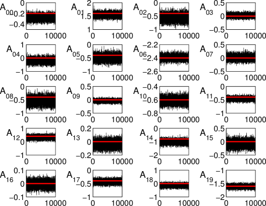
Figure 1: Output of a Gibbs sampler for $20$ drift parameters of a two dimensional model from Eq. (3). The observation interval is $\delta=10^{-3}$ and $T=10,000$. The true values are shown in red.

We performed a further simulation study to test the dependence of the posterior estimates upon the data set used. We inferred all of the drift parameters for a simple two dimensional model of the form of Eq. (3) using data sets of length $T=\{10,100,1000\}$ and with observation interval $\Delta=\{0.1,0.01,0.001\}$. Note that the diffusion function is arbitrary in this model. The results are shown in Table 1. For each parameter we estimated the posterior mean and the posterior 10th-90th percentiles. A cell is colored blue where the true value falls within this range. Note that if we were using the true likelihood, rather than an approximation, then we would expect there to be around $80\%$ blue boxes. The error of the estimates for each data set can be quantified using the quadratic Posterior Expected Loss (PEL) function

$$f(\hat{\pi},\bm{X}_{\mbox{\tiny{obs}}})=\int_{\Theta}(\bm{\theta}^{*}-\bm{\theta})^{2}\hat{\pi}(\bm{\theta}|\bm{X}_{\mbox{\tiny{obs}}})d\bm{\theta}\,,$$ (23)

where $\bm{\theta}$ represents all of the parameters, $\hat{\pi}$ is the estimated posterior distribution and $\bm{\theta}^{*}$ is the true value of the parameter.

	$T=10$			$T=100$			$T=1000$
	$\scriptstyle{0.1}$	$\scriptstyle{0.01}$	$\scriptstyle{0.001}$	$\scriptstyle{0.1}$	$\scriptstyle{0.01}$	$\scriptstyle{0.001}$	$\scriptstyle{0.1}$	$\scriptstyle{0.01}$	$\scriptstyle{0.001}$
$A_{00}=0$	$\begin{array}[]{c}\scriptscriptstyle{2.18}\\ \scriptscriptstyle{(-2.5,6.89)}\end{array}$	$\begin{array}[]{c}\scriptscriptstyle{-0.44}\\ \scriptscriptstyle{(-4.79,3.74)}\end{array}$	$\begin{array}[]{c}\scriptscriptstyle{-1.95}\\ \scriptscriptstyle{(-6.07,2.2)}\end{array}$	$\begin{array}[]{c}\scriptscriptstyle{-0.13}\\ \scriptscriptstyle{(-1.07,0.77)}\end{array}$	$\begin{array}[]{c}\scriptscriptstyle{0.65}\\ \scriptscriptstyle{(-0.29,1.6)}\end{array}$	$\begin{array}[]{c}\scriptscriptstyle{0.64}\\ \scriptscriptstyle{(-0.28,1.58)}\end{array}$	$\begin{array}[]{c}\scriptscriptstyle{0.02}\\ \scriptscriptstyle{(-0.13,0.17)}\end{array}$	$\begin{array}[]{c}\scriptscriptstyle{0.01}\\ \scriptscriptstyle{(-0.13,0.17)}\end{array}$	$\begin{array}[]{c}\scriptscriptstyle{0.02}\\ \scriptscriptstyle{(-0.13,0.18)}\end{array}$
$A_{01}=5$	$\begin{array}[]{c}\scriptscriptstyle{-2.04}\\ \scriptscriptstyle{(-7.23,3.04)}\end{array}$	$\begin{array}[]{c}\scriptscriptstyle{4.86}\\ \scriptscriptstyle{(0.84,9.04)}\end{array}$	$\begin{array}[]{c}\scriptscriptstyle{6.21}\\ \scriptscriptstyle{(2.31,10.12)}\end{array}$	$\begin{array}[]{c}\scriptscriptstyle{2.54}\\ \scriptscriptstyle{(1.78,3.28)}\end{array}$	$\begin{array}[]{c}\scriptscriptstyle{4.73}\\ \scriptscriptstyle{(3.93,5.51)}\end{array}$	$\begin{array}[]{c}\scriptscriptstyle{5.22}\\ \scriptscriptstyle{(4.43,6.03)}\end{array}$	$\begin{array}[]{c}\scriptscriptstyle{2.84}\\ \scriptscriptstyle{(2.7,2.97)}\end{array}$	$\begin{array}[]{c}\scriptscriptstyle{4.59}\\ \scriptscriptstyle{(4.45,4.73)}\end{array}$	$\begin{array}[]{c}\scriptscriptstyle{4.86}\\ \scriptscriptstyle{(4.73,5)}\end{array}$
$A_{02}=0$	$\begin{array}[]{c}\scriptscriptstyle{2.63}\\ \scriptscriptstyle{(-0.16,5.39)}\end{array}$	$\begin{array}[]{c}\scriptscriptstyle{2.15}\\ \scriptscriptstyle{(-0.17,4.49)}\end{array}$	$\begin{array}[]{c}\scriptscriptstyle{1.63}\\ \scriptscriptstyle{(-0.66,4)}\end{array}$	$\begin{array}[]{c}\scriptscriptstyle{0.45}\\ \scriptscriptstyle{(-0.52,1.41)}\end{array}$	$\begin{array}[]{c}\scriptscriptstyle{0.58}\\ \scriptscriptstyle{(-0.42,1.6)}\end{array}$	$\begin{array}[]{c}\scriptscriptstyle{0.13}\\ \scriptscriptstyle{(-0.89,1.13)}\end{array}$	$\begin{array}[]{c}\scriptscriptstyle{-0.08}\\ \scriptscriptstyle{(-0.22,0.05)}\end{array}$	$\begin{array}[]{c}\scriptscriptstyle{-0.14}\\ \scriptscriptstyle{(-0.27,0)}\end{array}$	$\begin{array}[]{c}\scriptscriptstyle{-0.19}\\ \scriptscriptstyle{(-0.32,-0.04)}\end{array}$
$A_{03}=0$	$\begin{array}[]{c}\scriptscriptstyle{1.54}\\ \scriptscriptstyle{(-2.75,5.84)}\end{array}$	$\begin{array}[]{c}\scriptscriptstyle{-0.17}\\ \scriptscriptstyle{(-3.12,2.76)}\end{array}$	$\begin{array}[]{c}\scriptscriptstyle{0.26}\\ \scriptscriptstyle{(-2.62,3.2)}\end{array}$	$\begin{array}[]{c}\scriptscriptstyle{0.27}\\ \scriptscriptstyle{(-0.38,0.93)}\end{array}$	$\begin{array}[]{c}\scriptscriptstyle{0.01}\\ \scriptscriptstyle{(-0.72,0.73)}\end{array}$	$\begin{array}[]{c}\scriptscriptstyle{-0.17}\\ \scriptscriptstyle{(-0.88,0.54)}\end{array}$	$\begin{array}[]{c}\scriptscriptstyle{-0.01}\\ \scriptscriptstyle{(-0.08,0.06)}\end{array}$	$\begin{array}[]{c}\scriptscriptstyle{0}\\ \scriptscriptstyle{(-0.07,0.06)}\end{array}$	$\begin{array}[]{c}\scriptscriptstyle{0}\\ \scriptscriptstyle{(-0.07,0.06)}\end{array}$
$A_{04}=0$	$\begin{array}[]{c}\scriptscriptstyle{-3.51}\\ \scriptscriptstyle{(-8.17,1.13)}\end{array}$	$\begin{array}[]{c}\scriptscriptstyle{0.61}\\ \scriptscriptstyle{(-3,4.3)}\end{array}$	$\begin{array}[]{c}\scriptscriptstyle{1.3}\\ \scriptscriptstyle{(-2.32,5.07)}\end{array}$	$\begin{array}[]{c}\scriptscriptstyle{-0.96}\\ \scriptscriptstyle{(-2.09,0.2)}\end{array}$	$\begin{array}[]{c}\scriptscriptstyle{-0.58}\\ \scriptscriptstyle{(-1.8,0.68)}\end{array}$	$\begin{array}[]{c}\scriptscriptstyle{-0.07}\\ \scriptscriptstyle{(-1.3,1.16)}\end{array}$	$\begin{array}[]{c}\scriptscriptstyle{-0.01}\\ \scriptscriptstyle{(-0.04,0.01)}\end{array}$	$\begin{array}[]{c}\scriptscriptstyle{-0.02}\\ \scriptscriptstyle{(-0.04,0.01)}\end{array}$	$\begin{array}[]{c}\scriptscriptstyle{-0.02}\\ \scriptscriptstyle{(-0.05,0.01)}\end{array}$
$A_{05}=0$	$\begin{array}[]{c}\scriptscriptstyle{0.32}\\ \scriptscriptstyle{(-2.19,2.81)}\end{array}$	$\begin{array}[]{c}\scriptscriptstyle{0}\\ \scriptscriptstyle{(-2.31,2.31)}\end{array}$	$\begin{array}[]{c}\scriptscriptstyle{0.19}\\ \scriptscriptstyle{(-2.11,2.49)}\end{array}$	$\begin{array}[]{c}\scriptscriptstyle{0.66}\\ \scriptscriptstyle{(-0.11,1.43)}\end{array}$	$\begin{array}[]{c}\scriptscriptstyle{0.02}\\ \scriptscriptstyle{(-0.79,0.84)}\end{array}$	$\begin{array}[]{c}\scriptscriptstyle{-0.27}\\ \scriptscriptstyle{(-1.05,0.55)}\end{array}$	$\begin{array}[]{c}\scriptscriptstyle{0}\\ \scriptscriptstyle{(-0.06,0.07)}\end{array}$	$\begin{array}[]{c}\scriptscriptstyle{0.01}\\ \scriptscriptstyle{(-0.06,0.07)}\end{array}$	$\begin{array}[]{c}\scriptscriptstyle{0}\\ \scriptscriptstyle{(-0.07,0.07)}\end{array}$
$A_{06}=-3$	$\begin{array}[]{c}\scriptscriptstyle{-0.88}\\ \scriptscriptstyle{(-2.96,1.24)}\end{array}$	$\begin{array}[]{c}\scriptscriptstyle{-2.58}\\ \scriptscriptstyle{(-4.3,-0.87)}\end{array}$	$\begin{array}[]{c}\scriptscriptstyle{-3.17}\\ \scriptscriptstyle{(-4.83,-1.49)}\end{array}$	$\begin{array}[]{c}\scriptscriptstyle{-1.8}\\ \scriptscriptstyle{(-2,-1.6)}\end{array}$	$\begin{array}[]{c}\scriptscriptstyle{-2.92}\\ \scriptscriptstyle{(-3.12,-2.71)}\end{array}$	$\begin{array}[]{c}\scriptscriptstyle{-3.05}\\ \scriptscriptstyle{(-3.25,-2.85)}\end{array}$	$\begin{array}[]{c}\scriptscriptstyle{-1.71}\\ \scriptscriptstyle{(-1.77,-1.65)}\end{array}$	$\begin{array}[]{c}\scriptscriptstyle{-2.75}\\ \scriptscriptstyle{(-2.81,-2.69)}\end{array}$	$\begin{array}[]{c}\scriptscriptstyle{-2.91}\\ \scriptscriptstyle{(-2.97,-2.85)}\end{array}$
$A_{07}=0$	$\begin{array}[]{c}\scriptscriptstyle{0.58}\\ \scriptscriptstyle{(-1.87,3.06)}\end{array}$	$\begin{array}[]{c}\scriptscriptstyle{-1.32}\\ \scriptscriptstyle{(-3.32,0.7)}\end{array}$	$\begin{array}[]{c}\scriptscriptstyle{-1.48}\\ \scriptscriptstyle{(-3.54,0.52)}\end{array}$	$\begin{array}[]{c}\scriptscriptstyle{0.05}\\ \scriptscriptstyle{(-0.49,0.58)}\end{array}$	$\begin{array}[]{c}\scriptscriptstyle{-0.07}\\ \scriptscriptstyle{(-0.66,0.51)}\end{array}$	$\begin{array}[]{c}\scriptscriptstyle{-0.22}\\ \scriptscriptstyle{(-0.79,0.37)}\end{array}$	$\begin{array}[]{c}\scriptscriptstyle{-0.02}\\ \scriptscriptstyle{(-0.07,0.04)}\end{array}$	$\begin{array}[]{c}\scriptscriptstyle{-0.01}\\ \scriptscriptstyle{(-0.06,0.05)}\end{array}$	$\begin{array}[]{c}\scriptscriptstyle{0}\\ \scriptscriptstyle{(-0.05,0.06)}\end{array}$
$A_{08}=0$	$\begin{array}[]{c}\scriptscriptstyle{-0.83}\\ \scriptscriptstyle{(-3,1.31)}\end{array}$	$\begin{array}[]{c}\scriptscriptstyle{-0.28}\\ \scriptscriptstyle{(-2.31,1.76)}\end{array}$	$\begin{array}[]{c}\scriptscriptstyle{-0.18}\\ \scriptscriptstyle{(-2.21,1.86)}\end{array}$	$\begin{array}[]{c}\scriptscriptstyle{-0.48}\\ \scriptscriptstyle{(-1.03,0.07)}\end{array}$	$\begin{array}[]{c}\scriptscriptstyle{-0.37}\\ \scriptscriptstyle{(-0.96,0.23)}\end{array}$	$\begin{array}[]{c}\scriptscriptstyle{-0.16}\\ \scriptscriptstyle{(-0.75,0.42)}\end{array}$	$\begin{array}[]{c}\scriptscriptstyle{-0.02}\\ \scriptscriptstyle{(-0.08,0.03)}\end{array}$	$\begin{array}[]{c}\scriptscriptstyle{-0.01}\\ \scriptscriptstyle{(-0.06,0.04)}\end{array}$	$\begin{array}[]{c}\scriptscriptstyle{-0.01}\\ \scriptscriptstyle{(-0.07,0.04)}\end{array}$
$A_{09}=0$	$\begin{array}[]{c}\scriptscriptstyle{0.71}\\ \scriptscriptstyle{(-0.11,1.53)}\end{array}$	$\begin{array}[]{c}\scriptscriptstyle{-0.4}\\ \scriptscriptstyle{(-1.16,0.38)}\end{array}$	$\begin{array}[]{c}\scriptscriptstyle{-0.49}\\ \scriptscriptstyle{(-1.26,0.27)}\end{array}$	$\begin{array}[]{c}\scriptscriptstyle{0.33}\\ \scriptscriptstyle{(-0.02,0.67)}\end{array}$	$\begin{array}[]{c}\scriptscriptstyle{0.04}\\ \scriptscriptstyle{(-0.3,0.39)}\end{array}$	$\begin{array}[]{c}\scriptscriptstyle{0.09}\\ \scriptscriptstyle{(-0.25,0.44)}\end{array}$	$\begin{array}[]{c}\scriptscriptstyle{0.08}\\ \scriptscriptstyle{(0.02,0.13)}\end{array}$	$\begin{array}[]{c}\scriptscriptstyle{0.1}\\ \scriptscriptstyle{(0.04,0.16)}\end{array}$	$\begin{array}[]{c}\scriptscriptstyle{0.12}\\ \scriptscriptstyle{(0.05,0.17)}\end{array}$
$A_{10}=0$	$\begin{array}[]{c}\scriptscriptstyle{-0.38}\\ \scriptscriptstyle{(-5.19,4.24)}\end{array}$	$\begin{array}[]{c}\scriptscriptstyle{-2.21}\\ \scriptscriptstyle{(-6.44,2.03)}\end{array}$	$\begin{array}[]{c}\scriptscriptstyle{-1.17}\\ \scriptscriptstyle{(-5.21,2.9)}\end{array}$	$\begin{array}[]{c}\scriptscriptstyle{-0.31}\\ \scriptscriptstyle{(-1.22,0.61)}\end{array}$	$\begin{array}[]{c}\scriptscriptstyle{-0.18}\\ \scriptscriptstyle{(-1.1,0.75)}\end{array}$	$\begin{array}[]{c}\scriptscriptstyle{0.06}\\ \scriptscriptstyle{(-0.89,0.99)}\end{array}$	$\begin{array}[]{c}\scriptscriptstyle{0.02}\\ \scriptscriptstyle{(-0.13,0.17)}\end{array}$	$\begin{array}[]{c}\scriptscriptstyle{0.05}\\ \scriptscriptstyle{(-0.1,0.2)}\end{array}$	$\begin{array}[]{c}\scriptscriptstyle{0.05}\\ \scriptscriptstyle{(-0.1,0.2)}\end{array}$
$A_{11}=0$	$\begin{array}[]{c}\scriptscriptstyle{-2.93}\\ \scriptscriptstyle{(-8.11,2.15)}\end{array}$	$\begin{array}[]{c}\scriptscriptstyle{2.42}\\ \scriptscriptstyle{(-1.64,6.48)}\end{array}$	$\begin{array}[]{c}\scriptscriptstyle{1.67}\\ \scriptscriptstyle{(-2.29,5.64)}\end{array}$	$\begin{array}[]{c}\scriptscriptstyle{0.88}\\ \scriptscriptstyle{(0.1,1.64)}\end{array}$	$\begin{array}[]{c}\scriptscriptstyle{0.39}\\ \scriptscriptstyle{(-0.4,1.19)}\end{array}$	$\begin{array}[]{c}\scriptscriptstyle{0.33}\\ \scriptscriptstyle{(-0.48,1.12)}\end{array}$	$\begin{array}[]{c}\scriptscriptstyle{-0.06}\\ \scriptscriptstyle{(-0.2,0.08)}\end{array}$	$\begin{array}[]{c}\scriptscriptstyle{0.11}\\ \scriptscriptstyle{(-0.03,0.25)}\end{array}$	$\begin{array}[]{c}\scriptscriptstyle{0.11}\\ \scriptscriptstyle{(-0.04,0.24)}\end{array}$
$A_{12}=5$	$\begin{array}[]{c}\scriptscriptstyle{5.96}\\ \scriptscriptstyle{(3.22,8.68)}\end{array}$	$\begin{array}[]{c}\scriptscriptstyle{4.2}\\ \scriptscriptstyle{(1.89,6.63)}\end{array}$	$\begin{array}[]{c}\scriptscriptstyle{4.72}\\ \scriptscriptstyle{(2.33,7.09)}\end{array}$	$\begin{array}[]{c}\scriptscriptstyle{1.68}\\ \scriptscriptstyle{(0.72,2.65)}\end{array}$	$\begin{array}[]{c}\scriptscriptstyle{4.56}\\ \scriptscriptstyle{(3.52,5.57)}\end{array}$	$\begin{array}[]{c}\scriptscriptstyle{5.09}\\ \scriptscriptstyle{(4.08,6.12)}\end{array}$	$\begin{array}[]{c}\scriptscriptstyle{2.88}\\ \scriptscriptstyle{(2.74,3.02)}\end{array}$	$\begin{array}[]{c}\scriptscriptstyle{4.7}\\ \scriptscriptstyle{(4.56,4.84)}\end{array}$	$\begin{array}[]{c}\scriptscriptstyle{4.98}\\ \scriptscriptstyle{(4.84,5.11)}\end{array}$
$A_{13}=0$	$\begin{array}[]{c}\scriptscriptstyle{2.68}\\ \scriptscriptstyle{(-1.67,6.93)}\end{array}$	$\begin{array}[]{c}\scriptscriptstyle{-1.41}\\ \scriptscriptstyle{(-4.36,1.57)}\end{array}$	$\begin{array}[]{c}\scriptscriptstyle{-1.88}\\ \scriptscriptstyle{(-4.74,1.02)}\end{array}$	$\begin{array}[]{c}\scriptscriptstyle{-1.05}\\ \scriptscriptstyle{(-1.72,-0.38)}\end{array}$	$\begin{array}[]{c}\scriptscriptstyle{-0.61}\\ \scriptscriptstyle{(-1.33,0.1)}\end{array}$	$\begin{array}[]{c}\scriptscriptstyle{-0.74}\\ \scriptscriptstyle{(-1.46,-0.02)}\end{array}$	$\begin{array}[]{c}\scriptscriptstyle{-0.01}\\ \scriptscriptstyle{(-0.08,0.05)}\end{array}$	$\begin{array}[]{c}\scriptscriptstyle{-0.03}\\ \scriptscriptstyle{(-0.1,0.03)}\end{array}$	$\begin{array}[]{c}\scriptscriptstyle{-0.03}\\ \scriptscriptstyle{(-0.09,0.04)}\end{array}$
$A_{14}=0$	$\begin{array}[]{c}\scriptscriptstyle{-1.13}\\ \scriptscriptstyle{(-5.84,3.6)}\end{array}$	$\begin{array}[]{c}\scriptscriptstyle{4.67}\\ \scriptscriptstyle{(1.01,8.45)}\end{array}$	$\begin{array}[]{c}\scriptscriptstyle{4.23}\\ \scriptscriptstyle{(0.47,7.92)}\end{array}$	$\begin{array}[]{c}\scriptscriptstyle{1.39}\\ \scriptscriptstyle{(0.24,2.55)}\end{array}$	$\begin{array}[]{c}\scriptscriptstyle{0.78}\\ \scriptscriptstyle{(-0.44,2.03)}\end{array}$	$\begin{array}[]{c}\scriptscriptstyle{0.91}\\ \scriptscriptstyle{(-0.33,2.14)}\end{array}$	$\begin{array}[]{c}\scriptscriptstyle{0.02}\\ \scriptscriptstyle{(-0.01,0.05)}\end{array}$	$\begin{array}[]{c}\scriptscriptstyle{0.03}\\ \scriptscriptstyle{(0,0.05)}\end{array}$	$\begin{array}[]{c}\scriptscriptstyle{0.03}\\ \scriptscriptstyle{(0,0.05)}\end{array}$
$A_{15}=0$	$\begin{array}[]{c}\scriptscriptstyle{0.42}\\ \scriptscriptstyle{(-2.07,2.94)}\end{array}$	$\begin{array}[]{c}\scriptscriptstyle{-0.6}\\ \scriptscriptstyle{(-2.88,1.77)}\end{array}$	$\begin{array}[]{c}\scriptscriptstyle{-0.84}\\ \scriptscriptstyle{(-3.13,1.45)}\end{array}$	$\begin{array}[]{c}\scriptscriptstyle{-0.22}\\ \scriptscriptstyle{(-1.01,0.56)}\end{array}$	$\begin{array}[]{c}\scriptscriptstyle{-0.11}\\ \scriptscriptstyle{(-0.9,0.7)}\end{array}$	$\begin{array}[]{c}\scriptscriptstyle{-0.24}\\ \scriptscriptstyle{(-1.06,0.55)}\end{array}$	$\begin{array}[]{c}\scriptscriptstyle{0}\\ \scriptscriptstyle{(-0.07,0.06)}\end{array}$	$\begin{array}[]{c}\scriptscriptstyle{-0.01}\\ \scriptscriptstyle{(-0.08,0.05)}\end{array}$	$\begin{array}[]{c}\scriptscriptstyle{-0.02}\\ \scriptscriptstyle{(-0.09,0.04)}\end{array}$
$A_{16}=0$	$\begin{array}[]{c}\scriptscriptstyle{-0.82}\\ \scriptscriptstyle{(-2.94,1.29)}\end{array}$	$\begin{array}[]{c}\scriptscriptstyle{0.12}\\ \scriptscriptstyle{(-1.61,1.83)}\end{array}$	$\begin{array}[]{c}\scriptscriptstyle{0.39}\\ \scriptscriptstyle{(-1.26,2)}\end{array}$	$\begin{array}[]{c}\scriptscriptstyle{-0.08}\\ \scriptscriptstyle{(-0.28,0.12)}\end{array}$	$\begin{array}[]{c}\scriptscriptstyle{-0.04}\\ \scriptscriptstyle{(-0.24,0.17)}\end{array}$	$\begin{array}[]{c}\scriptscriptstyle{-0.02}\\ \scriptscriptstyle{(-0.22,0.19)}\end{array}$	$\begin{array}[]{c}\scriptscriptstyle{-0.03}\\ \scriptscriptstyle{(-0.09,0.03)}\end{array}$	$\begin{array}[]{c}\scriptscriptstyle{-0.08}\\ \scriptscriptstyle{(-0.14,-0.02)}\end{array}$	$\begin{array}[]{c}\scriptscriptstyle{-0.09}\\ \scriptscriptstyle{(-0.15,-0.03)}\end{array}$
$A_{17}=0$	$\begin{array}[]{c}\scriptscriptstyle{-0.46}\\ \scriptscriptstyle{(-2.95,2.04)}\end{array}$	$\begin{array}[]{c}\scriptscriptstyle{-3.21}\\ \scriptscriptstyle{(-5.28,-1.22)}\end{array}$	$\begin{array}[]{c}\scriptscriptstyle{-2.97}\\ \scriptscriptstyle{(-4.99,-0.93)}\end{array}$	$\begin{array}[]{c}\scriptscriptstyle{-0.71}\\ \scriptscriptstyle{(-1.25,-0.17)}\end{array}$	$\begin{array}[]{c}\scriptscriptstyle{-0.66}\\ \scriptscriptstyle{(-1.24,-0.08)}\end{array}$	$\begin{array}[]{c}\scriptscriptstyle{-0.78}\\ \scriptscriptstyle{(-1.35,-0.19)}\end{array}$	$\begin{array}[]{c}\scriptscriptstyle{0.01}\\ \scriptscriptstyle{(-0.05,0.06)}\end{array}$	$\begin{array}[]{c}\scriptscriptstyle{-0.01}\\ \scriptscriptstyle{(-0.06,0.04)}\end{array}$	$\begin{array}[]{c}\scriptscriptstyle{0}\\ \scriptscriptstyle{(-0.05,0.05)}\end{array}$
$A_{18}=0$	$\begin{array}[]{c}\scriptscriptstyle{0.66}\\ \scriptscriptstyle{(-1.5,2.86)}\end{array}$	$\begin{array}[]{c}\scriptscriptstyle{1.33}\\ \scriptscriptstyle{(-0.71,3.35)}\end{array}$	$\begin{array}[]{c}\scriptscriptstyle{1.63}\\ \scriptscriptstyle{(-0.41,3.6)}\end{array}$	$\begin{array}[]{c}\scriptscriptstyle{0.65}\\ \scriptscriptstyle{(0.11,1.22)}\end{array}$	$\begin{array}[]{c}\scriptscriptstyle{0.45}\\ \scriptscriptstyle{(-0.13,1.04)}\end{array}$	$\begin{array}[]{c}\scriptscriptstyle{0.58}\\ \scriptscriptstyle{(-0.01,1.18)}\end{array}$	$\begin{array}[]{c}\scriptscriptstyle{0.06}\\ \scriptscriptstyle{(0.01,0.12)}\end{array}$	$\begin{array}[]{c}\scriptscriptstyle{0.02}\\ \scriptscriptstyle{(-0.03,0.08)}\end{array}$	$\begin{array}[]{c}\scriptscriptstyle{0.03}\\ \scriptscriptstyle{(-0.02,0.09)}\end{array}$
$A_{19}=-3$	$\begin{array}[]{c}\scriptscriptstyle{-2.61}\\ \scriptscriptstyle{(-3.44,-1.78)}\end{array}$	$\begin{array}[]{c}\scriptscriptstyle{-3.23}\\ \scriptscriptstyle{(-4.02,-2.45)}\end{array}$	$\begin{array}[]{c}\scriptscriptstyle{-3.47}\\ \scriptscriptstyle{(-4.24,-2.69)}\end{array}$	$\begin{array}[]{c}\scriptscriptstyle{-1.46}\\ \scriptscriptstyle{(-1.8,-1.12)}\end{array}$	$\begin{array}[]{c}\scriptscriptstyle{-2.73}\\ \scriptscriptstyle{(-3.07,-2.38)}\end{array}$	$\begin{array}[]{c}\scriptscriptstyle{-3.04}\\ \scriptscriptstyle{(-3.39,-2.7)}\end{array}$	$\begin{array}[]{c}\scriptscriptstyle{-1.75}\\ \scriptscriptstyle{(-1.81,-1.69)}\end{array}$	$\begin{array}[]{c}\scriptscriptstyle{-2.81}\\ \scriptscriptstyle{(-2.87,-2.75)}\end{array}$	$\begin{array}[]{c}\scriptscriptstyle{-2.98}\\ \scriptscriptstyle{(-3.04,-2.92)}\end{array}$
	8.48	5.25	4.96	1.19	0.37	0.36	0.43	0.02	0.01

Table 1: Drift parameter estimates for a two dimensional cubic model with arbitrary diffusion function. On the left is the true value of the parameter. The length of the data set used for the inference is labeled as $T$ and the observation interval is $\Delta=\{0.1,0.01,0.001\}$. In each cell the parameter is estimated from the posterior mean and in brackets is shown the 10th-90th percentiles of the posterior. The blue coloring is where the true value falls in this range. The bottom of the table shows the Posterior Expected Loss in each case.

We performed a test with both the Gibbs sampler and data imputation. In Tab. 2 the data is observed at interval $\Delta=0.1$. The smaller intervals $\Delta=\{0.01,0.001\}$ are obtained by imputing data with $m=\{10,100\}$ respectively. The table shows that imputing data approximately doubles the Posterior Expected Loss. As expected the confidence intervals are broader but with more imputed data the algorithm can recover the true values. This shows that our data imputing strategy successfully improves the parameter estimates.

	$T=10$			$T=100$			$T=1000$
	$\scriptstyle{0.1}$	$\scriptstyle{0.01}$	$\scriptstyle{0.001}$	$\scriptstyle{0.1}$	$\scriptstyle{0.01}$	$\scriptstyle{0.001}$	$\scriptstyle{0.1}$	$\scriptstyle{0.01}$	$\scriptstyle{0.001}$
$A_{00}=0$	$\begin{array}[]{c}\scriptscriptstyle{2.18}\\ \scriptscriptstyle{(-2.5,6.89)}\end{array}$	$\begin{array}[]{c}\scriptscriptstyle{-2.46}\\ \scriptscriptstyle{(-8.46,3.52)}\end{array}$	$\begin{array}[]{c}\scriptscriptstyle{-2.59}\\ \scriptscriptstyle{(-8.35,3.24)}\end{array}$	$\begin{array}[]{c}\scriptscriptstyle{-0.13}\\ \scriptscriptstyle{(-1.07,0.77)}\end{array}$	$\begin{array}[]{c}\scriptscriptstyle{-0.68}\\ \scriptscriptstyle{(-1.84,0.5)}\end{array}$	$\begin{array}[]{c}\scriptscriptstyle{-0.69}\\ \scriptscriptstyle{(-1.85,0.49)}\end{array}$	$\begin{array}[]{c}\scriptscriptstyle{0.02}\\ \scriptscriptstyle{(-0.13,0.17)}\end{array}$	$\begin{array}[]{c}\scriptscriptstyle{-0.08}\\ \scriptscriptstyle{(-0.27,0.09)}\end{array}$	$\begin{array}[]{c}\scriptscriptstyle{-0.08}\\ \scriptscriptstyle{(-0.26,0.09)}\end{array}$
$A_{01}=5$	$\begin{array}[]{c}\scriptscriptstyle{-2.04}\\ \scriptscriptstyle{(-7.23,3.04)}\end{array}$	$\begin{array}[]{c}\scriptscriptstyle{4.99}\\ \scriptscriptstyle{(-0.7,10.61)}\end{array}$	$\begin{array}[]{c}\scriptscriptstyle{4.84}\\ \scriptscriptstyle{(-0.49,10.22)}\end{array}$	$\begin{array}[]{c}\scriptscriptstyle{2.54}\\ \scriptscriptstyle{(1.78,3.28)}\end{array}$	$\begin{array}[]{c}\scriptscriptstyle{4.89}\\ \scriptscriptstyle{(3.83,5.97)}\end{array}$	$\begin{array}[]{c}\scriptscriptstyle{4.76}\\ \scriptscriptstyle{(3.74,5.79)}\end{array}$	$\begin{array}[]{c}\scriptscriptstyle{2.84}\\ \scriptscriptstyle{(2.7,2.97)}\end{array}$	$\begin{array}[]{c}\scriptscriptstyle{5.04}\\ \scriptscriptstyle{(4.87,5.21)}\end{array}$	$\begin{array}[]{c}\scriptscriptstyle{4.88}\\ \scriptscriptstyle{(4.71,5.03)}\end{array}$
$A_{02}=0$	$\begin{array}[]{c}\scriptscriptstyle{2.63}\\ \scriptscriptstyle{(-0.16,5.39)}\end{array}$	$\begin{array}[]{c}\scriptscriptstyle{0.61}\\ \scriptscriptstyle{(-2.94,4.05)}\end{array}$	$\begin{array}[]{c}\scriptscriptstyle{0.39}\\ \scriptscriptstyle{(-2.95,3.75)}\end{array}$	$\begin{array}[]{c}\scriptscriptstyle{0.45}\\ \scriptscriptstyle{(-0.52,1.41)}\end{array}$	$\begin{array}[]{c}\scriptscriptstyle{-0.06}\\ \scriptscriptstyle{(-1.42,1.3)}\end{array}$	$\begin{array}[]{c}\scriptscriptstyle{-0.2}\\ \scriptscriptstyle{(-1.49,1.13)}\end{array}$	$\begin{array}[]{c}\scriptscriptstyle{-0.08}\\ \scriptscriptstyle{(-0.22,0.05)}\end{array}$	$\begin{array}[]{c}\scriptscriptstyle{-0.26}\\ \scriptscriptstyle{(-0.44,-0.08)}\end{array}$	$\begin{array}[]{c}\scriptscriptstyle{-0.28}\\ \scriptscriptstyle{(-0.45,-0.09)}\end{array}$
$A_{03}=0$	$\begin{array}[]{c}\scriptscriptstyle{1.54}\\ \scriptscriptstyle{(-2.75,5.84)}\end{array}$	$\begin{array}[]{c}\scriptscriptstyle{3.25}\\ \scriptscriptstyle{(-1.23,8.07)}\end{array}$	$\begin{array}[]{c}\scriptscriptstyle{3.26}\\ \scriptscriptstyle{(-1.07,7.77)}\end{array}$	$\begin{array}[]{c}\scriptscriptstyle{0.27}\\ \scriptscriptstyle{(-0.38,0.93)}\end{array}$	$\begin{array}[]{c}\scriptscriptstyle{0.67}\\ \scriptscriptstyle{(-0.34,1.67)}\end{array}$	$\begin{array}[]{c}\scriptscriptstyle{0.59}\\ \scriptscriptstyle{(-0.41,1.59)}\end{array}$	$\begin{array}[]{c}\scriptscriptstyle{-0.01}\\ \scriptscriptstyle{(-0.08,0.06)}\end{array}$	$\begin{array}[]{c}\scriptscriptstyle{0.02}\\ \scriptscriptstyle{(-0.06,0.1)}\end{array}$	$\begin{array}[]{c}\scriptscriptstyle{0.02}\\ \scriptscriptstyle{(-0.06,0.09)}\end{array}$
$A_{04}=0$	$\begin{array}[]{c}\scriptscriptstyle{-3.51}\\ \scriptscriptstyle{(-8.17,1.13)}\end{array}$	$\begin{array}[]{c}\scriptscriptstyle{-2.53}\\ \scriptscriptstyle{(-7.76,2.61)}\end{array}$	$\begin{array}[]{c}\scriptscriptstyle{-2.53}\\ \scriptscriptstyle{(-7.61,2.41)}\end{array}$	$\begin{array}[]{c}\scriptscriptstyle{-0.96}\\ \scriptscriptstyle{(-2.09,0.2)}\end{array}$	$\begin{array}[]{c}\scriptscriptstyle{-1.6}\\ \scriptscriptstyle{(-3.35,0.18)}\end{array}$	$\begin{array}[]{c}\scriptscriptstyle{-1.41}\\ \scriptscriptstyle{(-3.14,0.27)}\end{array}$	$\begin{array}[]{c}\scriptscriptstyle{-0.01}\\ \scriptscriptstyle{(-0.04,0.01)}\end{array}$	$\begin{array}[]{c}\scriptscriptstyle{-0.03}\\ \scriptscriptstyle{(-0.05,0)}\end{array}$	$\begin{array}[]{c}\scriptscriptstyle{-0.02}\\ \scriptscriptstyle{(-0.05,0)}\end{array}$
$A_{05}=0$	$\begin{array}[]{c}\scriptscriptstyle{0.32}\\ \scriptscriptstyle{(-2.19,2.81)}\end{array}$	$\begin{array}[]{c}\scriptscriptstyle{1.85}\\ \scriptscriptstyle{(-1.6,5.2)}\end{array}$	$\begin{array}[]{c}\scriptscriptstyle{1.85}\\ \scriptscriptstyle{(-1.43,5.11)}\end{array}$	$\begin{array}[]{c}\scriptscriptstyle{0.66}\\ \scriptscriptstyle{(-0.11,1.43)}\end{array}$	$\begin{array}[]{c}\scriptscriptstyle{1.18}\\ \scriptscriptstyle{(0.03,2.32)}\end{array}$	$\begin{array}[]{c}\scriptscriptstyle{1.12}\\ \scriptscriptstyle{(-0.02,2.25)}\end{array}$	$\begin{array}[]{c}\scriptscriptstyle{0}\\ \scriptscriptstyle{(-0.06,0.07)}\end{array}$	$\begin{array}[]{c}\scriptscriptstyle{0.05}\\ \scriptscriptstyle{(-0.04,0.13)}\end{array}$	$\begin{array}[]{c}\scriptscriptstyle{0.05}\\ \scriptscriptstyle{(-0.04,0.13)}\end{array}$
$A_{06}=-3$	$\begin{array}[]{c}\scriptscriptstyle{-0.88}\\ \scriptscriptstyle{(-2.96,1.24)}\end{array}$	$\begin{array}[]{c}\scriptscriptstyle{-4.06}\\ \scriptscriptstyle{(-6.63,-1.76)}\end{array}$	$\begin{array}[]{c}\scriptscriptstyle{-4.02}\\ \scriptscriptstyle{(-6.5,-1.79)}\end{array}$	$\begin{array}[]{c}\scriptscriptstyle{-1.8}\\ \scriptscriptstyle{(-2,-1.6)}\end{array}$	$\begin{array}[]{c}\scriptscriptstyle{-3.19}\\ \scriptscriptstyle{(-3.44,-2.94)}\end{array}$	$\begin{array}[]{c}\scriptscriptstyle{-3.06}\\ \scriptscriptstyle{(-3.3,-2.83)}\end{array}$	$\begin{array}[]{c}\scriptscriptstyle{-1.71}\\ \scriptscriptstyle{(-1.77,-1.65)}\end{array}$	$\begin{array}[]{c}\scriptscriptstyle{-3.01}\\ \scriptscriptstyle{(-3.08,-2.94)}\end{array}$	$\begin{array}[]{c}\scriptscriptstyle{-2.92}\\ \scriptscriptstyle{(-2.98,-2.85)}\end{array}$
$A_{07}=0$	$\begin{array}[]{c}\scriptscriptstyle{0.58}\\ \scriptscriptstyle{(-1.87,3.06)}\end{array}$	$\begin{array}[]{c}\scriptscriptstyle{0.44}\\ \scriptscriptstyle{(-2.27,3.17)}\end{array}$	$\begin{array}[]{c}\scriptscriptstyle{0.53}\\ \scriptscriptstyle{(-2.05,3.23)}\end{array}$	$\begin{array}[]{c}\scriptscriptstyle{0.05}\\ \scriptscriptstyle{(-0.49,0.58)}\end{array}$	$\begin{array}[]{c}\scriptscriptstyle{0.43}\\ \scriptscriptstyle{(-0.37,1.27)}\end{array}$	$\begin{array}[]{c}\scriptscriptstyle{0.39}\\ \scriptscriptstyle{(-0.42,1.19)}\end{array}$	$\begin{array}[]{c}\scriptscriptstyle{-0.02}\\ \scriptscriptstyle{(-0.07,0.04)}\end{array}$	$\begin{array}[]{c}\scriptscriptstyle{0.03}\\ \scriptscriptstyle{(-0.04,0.09)}\end{array}$	$\begin{array}[]{c}\scriptscriptstyle{0.03}\\ \scriptscriptstyle{(-0.03,0.09)}\end{array}$
$A_{08}=0$	$\begin{array}[]{c}\scriptscriptstyle{-0.83}\\ \scriptscriptstyle{(-3,1.31)}\end{array}$	$\begin{array}[]{c}\scriptscriptstyle{-2.22}\\ \scriptscriptstyle{(-4.98,0.62)}\end{array}$	$\begin{array}[]{c}\scriptscriptstyle{-2.12}\\ \scriptscriptstyle{(-4.84,0.65)}\end{array}$	$\begin{array}[]{c}\scriptscriptstyle{-0.48}\\ \scriptscriptstyle{(-1.03,0.07)}\end{array}$	$\begin{array}[]{c}\scriptscriptstyle{-1}\\ \scriptscriptstyle{(-1.86,-0.14)}\end{array}$	$\begin{array}[]{c}\scriptscriptstyle{-0.92}\\ \scriptscriptstyle{(-1.76,-0.09)}\end{array}$	$\begin{array}[]{c}\scriptscriptstyle{-0.02}\\ \scriptscriptstyle{(-0.08,0.03)}\end{array}$	$\begin{array}[]{c}\scriptscriptstyle{-0.02}\\ \scriptscriptstyle{(-0.09,0.05)}\end{array}$	$\begin{array}[]{c}\scriptscriptstyle{-0.02}\\ \scriptscriptstyle{(-0.09,0.05)}\end{array}$
$A_{09}=0$	$\begin{array}[]{c}\scriptscriptstyle{0.71}\\ \scriptscriptstyle{(-0.11,1.53)}\end{array}$	$\begin{array}[]{c}\scriptscriptstyle{1.29}\\ \scriptscriptstyle{(0.06,2.61)}\end{array}$	$\begin{array}[]{c}\scriptscriptstyle{1.33}\\ \scriptscriptstyle{(0.1,2.6)}\end{array}$	$\begin{array}[]{c}\scriptscriptstyle{0.33}\\ \scriptscriptstyle{(-0.02,0.67)}\end{array}$	$\begin{array}[]{c}\scriptscriptstyle{0.7}\\ \scriptscriptstyle{(0.17,1.2)}\end{array}$	$\begin{array}[]{c}\scriptscriptstyle{0.71}\\ \scriptscriptstyle{(0.19,1.2)}\end{array}$	$\begin{array}[]{c}\scriptscriptstyle{0.08}\\ \scriptscriptstyle{(0.02,0.13)}\end{array}$	$\begin{array}[]{c}\scriptscriptstyle{0.14}\\ \scriptscriptstyle{(0.05,0.23)}\end{array}$	$\begin{array}[]{c}\scriptscriptstyle{0.15}\\ \scriptscriptstyle{(0.06,0.23)}\end{array}$
$A_{10}=0$	$\begin{array}[]{c}\scriptscriptstyle{-0.38}\\ \scriptscriptstyle{(-5.19,4.24)}\end{array}$	$\begin{array}[]{c}\scriptscriptstyle{-4.63}\\ \scriptscriptstyle{(-10.46,0.84)}\end{array}$	$\begin{array}[]{c}\scriptscriptstyle{-4.46}\\ \scriptscriptstyle{(-10.07,0.86)}\end{array}$	$\begin{array}[]{c}\scriptscriptstyle{-0.31}\\ \scriptscriptstyle{(-1.22,0.61)}\end{array}$	$\begin{array}[]{c}\scriptscriptstyle{0.66}\\ \scriptscriptstyle{(-0.55,1.87)}\end{array}$	$\begin{array}[]{c}\scriptscriptstyle{0.6}\\ \scriptscriptstyle{(-0.51,1.75)}\end{array}$	$\begin{array}[]{c}\scriptscriptstyle{0.02}\\ \scriptscriptstyle{(-0.13,0.17)}\end{array}$	$\begin{array}[]{c}\scriptscriptstyle{-0.02}\\ \scriptscriptstyle{(-0.2,0.16)}\end{array}$	$\begin{array}[]{c}\scriptscriptstyle{-0.01}\\ \scriptscriptstyle{(-0.2,0.16)}\end{array}$
$A_{11}=0$	$\begin{array}[]{c}\scriptscriptstyle{-2.93}\\ \scriptscriptstyle{(-8.11,2.15)}\end{array}$	$\begin{array}[]{c}\scriptscriptstyle{2.18}\\ \scriptscriptstyle{(-3.8,8.3)}\end{array}$	$\begin{array}[]{c}\scriptscriptstyle{2.24}\\ \scriptscriptstyle{(-3.53,8.27)}\end{array}$	$\begin{array}[]{c}\scriptscriptstyle{0.88}\\ \scriptscriptstyle{(0.1,1.64)}\end{array}$	$\begin{array}[]{c}\scriptscriptstyle{0.1}\\ \scriptscriptstyle{(-0.89,1.09)}\end{array}$	$\begin{array}[]{c}\scriptscriptstyle{0.15}\\ \scriptscriptstyle{(-0.82,1.14)}\end{array}$	$\begin{array}[]{c}\scriptscriptstyle{-0.06}\\ \scriptscriptstyle{(-0.2,0.08)}\end{array}$	$\begin{array}[]{c}\scriptscriptstyle{0.08}\\ \scriptscriptstyle{(-0.09,0.26)}\end{array}$	$\begin{array}[]{c}\scriptscriptstyle{0.11}\\ \scriptscriptstyle{(-0.06,0.29)}\end{array}$
$A_{12}=5$	$\begin{array}[]{c}\scriptscriptstyle{5.96}\\ \scriptscriptstyle{(3.22,8.68)}\end{array}$	$\begin{array}[]{c}\scriptscriptstyle{8.28}\\ \scriptscriptstyle{(4.62,11.9)}\end{array}$	$\begin{array}[]{c}\scriptscriptstyle{7.82}\\ \scriptscriptstyle{(4.39,11.36)}\end{array}$	$\begin{array}[]{c}\scriptscriptstyle{1.68}\\ \scriptscriptstyle{(0.72,2.65)}\end{array}$	$\begin{array}[]{c}\scriptscriptstyle{5.8}\\ \scriptscriptstyle{(4.52,7.07)}\end{array}$	$\begin{array}[]{c}\scriptscriptstyle{5.57}\\ \scriptscriptstyle{(4.36,6.81)}\end{array}$	$\begin{array}[]{c}\scriptscriptstyle{2.88}\\ \scriptscriptstyle{(2.74,3.02)}\end{array}$	$\begin{array}[]{c}\scriptscriptstyle{5.05}\\ \scriptscriptstyle{(4.88,5.22)}\end{array}$	$\begin{array}[]{c}\scriptscriptstyle{4.89}\\ \scriptscriptstyle{(4.72,5.05)}\end{array}$
$A_{13}=0$	$\begin{array}[]{c}\scriptscriptstyle{2.68}\\ \scriptscriptstyle{(-1.67,6.93)}\end{array}$	$\begin{array}[]{c}\scriptscriptstyle{4.03}\\ \scriptscriptstyle{(-0.84,9.1)}\end{array}$	$\begin{array}[]{c}\scriptscriptstyle{4.08}\\ \scriptscriptstyle{(-0.63,8.96)}\end{array}$	$\begin{array}[]{c}\scriptscriptstyle{-1.05}\\ \scriptscriptstyle{(-1.72,-0.38)}\end{array}$	$\begin{array}[]{c}\scriptscriptstyle{-0.83}\\ \scriptscriptstyle{(-1.76,0.11)}\end{array}$	$\begin{array}[]{c}\scriptscriptstyle{-0.81}\\ \scriptscriptstyle{(-1.72,0.1)}\end{array}$	$\begin{array}[]{c}\scriptscriptstyle{-0.01}\\ \scriptscriptstyle{(-0.08,0.05)}\end{array}$	$\begin{array}[]{c}\scriptscriptstyle{-0.01}\\ \scriptscriptstyle{(-0.09,0.08)}\end{array}$	$\begin{array}[]{c}\scriptscriptstyle{-0.01}\\ \scriptscriptstyle{(-0.09,0.08)}\end{array}$
$A_{14}=0$	$\begin{array}[]{c}\scriptscriptstyle{-1.13}\\ \scriptscriptstyle{(-5.84,3.6)}\end{array}$	$\begin{array}[]{c}\scriptscriptstyle{0.2}\\ \scriptscriptstyle{(-5.79,6.51)}\end{array}$	$\begin{array}[]{c}\scriptscriptstyle{0.02}\\ \scriptscriptstyle{(-5.85,6.12)}\end{array}$	$\begin{array}[]{c}\scriptscriptstyle{1.39}\\ \scriptscriptstyle{(0.24,2.55)}\end{array}$	$\begin{array}[]{c}\scriptscriptstyle{0.12}\\ \scriptscriptstyle{(-1.44,1.66)}\end{array}$	$\begin{array}[]{c}\scriptscriptstyle{0.07}\\ \scriptscriptstyle{(-1.43,1.61)}\end{array}$	$\begin{array}[]{c}\scriptscriptstyle{0.02}\\ \scriptscriptstyle{(-0.01,0.05)}\end{array}$	$\begin{array}[]{c}\scriptscriptstyle{0.03}\\ \scriptscriptstyle{(0,0.06)}\end{array}$	$\begin{array}[]{c}\scriptscriptstyle{0.03}\\ \scriptscriptstyle{(0,0.06)}\end{array}$
$A_{15}=0$	$\begin{array}[]{c}\scriptscriptstyle{0.42}\\ \scriptscriptstyle{(-2.07,2.94)}\end{array}$	$\begin{array}[]{c}\scriptscriptstyle{1.49}\\ \scriptscriptstyle{(-1.84,5)}\end{array}$	$\begin{array}[]{c}\scriptscriptstyle{1.59}\\ \scriptscriptstyle{(-1.64,4.85)}\end{array}$	$\begin{array}[]{c}\scriptscriptstyle{-0.22}\\ \scriptscriptstyle{(-1.01,0.56)}\end{array}$	$\begin{array}[]{c}\scriptscriptstyle{0.15}\\ \scriptscriptstyle{(-0.89,1.18)}\end{array}$	$\begin{array}[]{c}\scriptscriptstyle{0.2}\\ \scriptscriptstyle{(-0.8,1.19)}\end{array}$	$\begin{array}[]{c}\scriptscriptstyle{0}\\ \scriptscriptstyle{(-0.07,0.06)}\end{array}$	$\begin{array}[]{c}\scriptscriptstyle{0.01}\\ \scriptscriptstyle{(-0.07,0.08)}\end{array}$	$\begin{array}[]{c}\scriptscriptstyle{0}\\ \scriptscriptstyle{(-0.07,0.08)}\end{array}$
$A_{16}=0$	$\begin{array}[]{c}\scriptscriptstyle{-0.82}\\ \scriptscriptstyle{(-2.94,1.29)}\end{array}$	$\begin{array}[]{c}\scriptscriptstyle{-3.07}\\ \scriptscriptstyle{(-5.88,-0.39)}\end{array}$	$\begin{array}[]{c}\scriptscriptstyle{-3.14}\\ \scriptscriptstyle{(-5.86,-0.5)}\end{array}$	$\begin{array}[]{c}\scriptscriptstyle{-0.08}\\ \scriptscriptstyle{(-0.28,0.12)}\end{array}$	$\begin{array}[]{c}\scriptscriptstyle{-0.15}\\ \scriptscriptstyle{(-0.45,0.15)}\end{array}$	$\begin{array}[]{c}\scriptscriptstyle{-0.15}\\ \scriptscriptstyle{(-0.45,0.15)}\end{array}$	$\begin{array}[]{c}\scriptscriptstyle{-0.03}\\ \scriptscriptstyle{(-0.09,0.03)}\end{array}$	$\begin{array}[]{c}\scriptscriptstyle{-0.07}\\ \scriptscriptstyle{(-0.15,0.02)}\end{array}$	$\begin{array}[]{c}\scriptscriptstyle{-0.08}\\ \scriptscriptstyle{(-0.17,0)}\end{array}$
$A_{17}=0$	$\begin{array}[]{c}\scriptscriptstyle{-0.46}\\ \scriptscriptstyle{(-2.95,2.04)}\end{array}$	$\begin{array}[]{c}\scriptscriptstyle{-1.37}\\ \scriptscriptstyle{(-4.65,1.87)}\end{array}$	$\begin{array}[]{c}\scriptscriptstyle{-1.17}\\ \scriptscriptstyle{(-4.45,1.91)}\end{array}$	$\begin{array}[]{c}\scriptscriptstyle{-0.71}\\ \scriptscriptstyle{(-1.25,-0.17)}\end{array}$	$\begin{array}[]{c}\scriptscriptstyle{-0.59}\\ \scriptscriptstyle{(-1.36,0.19)}\end{array}$	$\begin{array}[]{c}\scriptscriptstyle{-0.57}\\ \scriptscriptstyle{(-1.31,0.17)}\end{array}$	$\begin{array}[]{c}\scriptscriptstyle{0.01}\\ \scriptscriptstyle{(-0.05,0.06)}\end{array}$	$\begin{array}[]{c}\scriptscriptstyle{0.05}\\ \scriptscriptstyle{(-0.02,0.12)}\end{array}$	$\begin{array}[]{c}\scriptscriptstyle{0.05}\\ \scriptscriptstyle{(-0.03,0.12)}\end{array}$
$A_{18}=0$	$\begin{array}[]{c}\scriptscriptstyle{0.66}\\ \scriptscriptstyle{(-1.5,2.86)}\end{array}$	$\begin{array}[]{c}\scriptscriptstyle{0.3}\\ \scriptscriptstyle{(-2.65,3.15)}\end{array}$	$\begin{array}[]{c}\scriptscriptstyle{-0.01}\\ \scriptscriptstyle{(-2.73,2.67)}\end{array}$	$\begin{array}[]{c}\scriptscriptstyle{0.65}\\ \scriptscriptstyle{(0.11,1.22)}\end{array}$	$\begin{array}[]{c}\scriptscriptstyle{0.24}\\ \scriptscriptstyle{(-0.51,0.99)}\end{array}$	$\begin{array}[]{c}\scriptscriptstyle{0.18}\\ \scriptscriptstyle{(-0.54,0.92)}\end{array}$	$\begin{array}[]{c}\scriptscriptstyle{0.06}\\ \scriptscriptstyle{(0.01,0.12)}\end{array}$	$\begin{array}[]{c}\scriptscriptstyle{0.02}\\ \scriptscriptstyle{(-0.04,0.08)}\end{array}$	$\begin{array}[]{c}\scriptscriptstyle{0.02}\\ \scriptscriptstyle{(-0.04,0.08)}\end{array}$
$A_{19}=-3$	$\begin{array}[]{c}\scriptscriptstyle{-2.61}\\ \scriptscriptstyle{(-3.44,-1.78)}\end{array}$	$\begin{array}[]{c}\scriptscriptstyle{-4.44}\\ \scriptscriptstyle{(-5.58,-3.38)}\end{array}$	$\begin{array}[]{c}\scriptscriptstyle{-4.1}\\ \scriptscriptstyle{(-5.16,-3.13)}\end{array}$	$\begin{array}[]{c}\scriptscriptstyle{-1.46}\\ \scriptscriptstyle{(-1.8,-1.12)}\end{array}$	$\begin{array}[]{c}\scriptscriptstyle{-3.09}\\ \scriptscriptstyle{(-3.53,-2.66)}\end{array}$	$\begin{array}[]{c}\scriptscriptstyle{-2.94}\\ \scriptscriptstyle{(-3.36,-2.55)}\end{array}$	$\begin{array}[]{c}\scriptscriptstyle{-1.75}\\ \scriptscriptstyle{(-1.81,-1.69)}\end{array}$	$\begin{array}[]{c}\scriptscriptstyle{-3.06}\\ \scriptscriptstyle{(-3.14,-2.99)}\end{array}$	$\begin{array}[]{c}\scriptscriptstyle{-2.97}\\ \scriptscriptstyle{(-3.04,-2.9)}\end{array}$
	8.48	11.06	10.32	1.19	0.76	0.68	0.43	0.01	0.01

Table 2: Drift parameter estimates for a two dimensional cubic model with arbitrary diffusion function. On the left is the true value of the parameter. The data used is the same as that of Table 1 sampled at the $\Delta=0.1$ interval. In this case data is imputed to obtain the intervals $\Delta=\{0.01,0.001\}$. The bottom of the table shows the Posterior Expected Loss in each case.

Our aim is to infer models that can be used for prediction. This can be problematic when dealing with non-linear models as some (generally unknown) regions of the parameter space will give solutions that explode to infinity with probability 1. This is a particular problem when, as exemplified by Table 1, large amounts of data are needed to regain the true values.

To demonstrate this problem we performed an inference on a two dimensional cubic model using $N=1,000$ observations at $\Delta=0.1$. For each inferred parameter value we then simulated the solution for $T=100$. After this time we recorded whether the solution retained finite values or had exploded. The marginal posterior distributions of the cubic parameters are plotted in Fig. 2. Each plot shows two histograms: one in blue records the distribution of stable parameter values and in red are those that exploded. Notice that, when looking at the marginal distributions, the stable and unstable regions largely overlap; it is difficult to separate the two regions. In this case $40\%$ of values were unstable. Tests (not shown) indicate that this is an even bigger problem in higher dimensions. Therefore, it is essential to use constraints on the parameter space to enable only physically meaningful solutions. The necessary conditions have been derived in section 2.

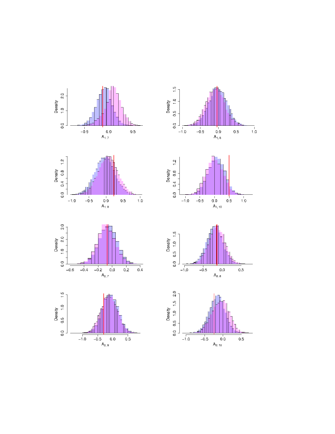
Figure 2: Marginal distributions of the cubic parameters inferred from a data set with $N=1,000$ observations at interval $\Delta=0.1$. The blue histogram shows the parameters that gave stable solutions to the SDE, while the red is for those that gave unstable solutions. The true values are given by the red lines.

Thus, as shown above, when updating the drift parameters we ensure that $\bm{M}$ is negative definite. In practice it is sufficient to check only whether the symmetric part $(\bm{M}+\bm{M}^{T})/2$ is negative-definite. In the next section we will develop a systematic way of sampling negative definite matrices.

3.3 Sampling Negative Definite Matrices

To sample negative definite matrices we use the Component Wise algorithm (32). Here we sample the density of a $n\times n$ matrix $\bm{M}$, with normally distributed components, subject to the constraint that it is negative definite. This algorithm updates $\bm{M}$ component wise and is based on the following property: a $n\times n$ matrix is negative definite if and only if all $k\leq n$ leading principal minors obey $|\bm{M}^{(k)}|(-1)^{k}>0$. The $k$th principal minor is the determinant of the upper left $k\times k$ sub-matrix. Consider the parameters along the main diagonal. As they only enter $\bm{M}$ once, each will have an associated upper bound. The Algorithm 3 works by calculating the upper bound associated with the constraints from each principal minor. It does this to find the least upper bound and thereby the truncation point of the normal distribution.

Algorithm 3 Sample parameters along diagonal

  for $i=1$ to $n$ do

     $U_{i}$=0

     for $j=i$ to $n$ do

        $x=-\left(\sum_{\mbox{\tiny$\begin{array}[]{c}k\neq i\\ k=1\end{array}$}}^{j}(-1)^{i+k}M_{ik}|M^{(j)}_{\{-i\},\{-k\}}|\right)/|M^{(j)}_{\{-i\},\{-i\}}|$

     end for

     if $x<U_{i}$ then

        $U_{i}=x$

     end if

     $M_{ii}\sim\mathcal{N}_{-}(\mu_{i},U_{i},\sigma^{2}_{i})$

  end for

Here, $\mathcal{N}_{-}(\mu,u,\sigma^{2})$ is the right truncated normal distribution with mean $\mu$, standard deviation $\sigma$ and upper bound $u$. The off-diagonal parameters enter twice so there will be a quadratic function determining their limits for each leading principal minor. For parameters in element $M^{(k)}_{ij}$ there will be an associated quadratic relation $a^{(k)}_{ij}M_{ij}^{2}+b^{(k)}_{ij}M_{ij}+c^{(k)}_{ij}=0$ where the coefficients are functions of the other parameters. These coefficients are found to be

$$a^{(k)}_{ij} = -|M^{(k)}_{/\{i,j\},/\{i,j\}}|$$ (24a)

$$b^{(k)}_{ij} = (-1)^{i+j}\sum_{\mbox{\tiny$\begin{array}[]{c}k\neq i\\ k=1\end{array}$}}^{j-1}M_{jk}(-1)^{j-1+k}|M^{(k)}_{/\{i,j\},/\{j,k\}}|$$ (24g)

$$+(-1)^{i+j}\sum_{\mbox{\tiny$\begin{array}[]{c}k\neq i\\ k=j+1\end{array}$}}^{N}M_{jk}(-1)^{j+k}|M^{(k)}_{/\{i,j\},/\{j,k\}}|$$

$$+ (-1)^{i+j}\sum_{\mbox{\tiny$\begin{array}[]{c}k\neq j\\ k=1\end{array}$}}^{i-1}M_{ik}(-1)^{i-1+k}|M^{(k)}_{/\{i,j\},/\{i,k\}}|$$ (24m)

$$+(-1)^{i+j}\sum_{\mbox{\tiny$\begin{array}[]{c}k\neq j\\ k=i+1\end{array}$}}^{N}M_{ik}(-1)^{i+k}|M^{(k)}_{/\{i,j\},/\{i,k\}}|$$

$$c^{(k)}_{ij} = \sum_{\mbox{\tiny$\begin{array}[]{c}k\neq j\\ k=1\end{array}$}}^{N}M_{ik}(-1)^{i+k}\left(\sum_{\mbox{\tiny$\begin{array}[]{c}l\neq i\\ l=1\end{array}$}}^{k-1}M_{jl}(-1)^{j-1+l}|M^{(k)}_{/\{i,j\},/\{l,k\}}|+\right.$$ (24u)

$$\left.\sum_{\mbox{\tiny$\begin{array}[]{c}l\neq i\\ l=k+1\end{array}$}}^{N}M_{jl}(-1)^{j+l}|M^{(k)}_{/\{i,j\},/\{l,k\}}|\right),$$

where $|M^{(k)}_{/\{i,j\},/\{l,k\}}|$ represents the $k$th principal minor with rows $i$ and $j$ and columns $l$ and $k$ removed. For each component $M_{ij}$ this quadratic form can be solved to give upper and lower bounds on the parameter. The matrix $\bm{M}$ can be cycled through updating each parameter in turn. Algorithm 4 describes the sampling of off-diagonal elements using the coefficients in Eq. (24u). Here, the notation, $\mathcal{N}_{-}^{+}(\mu,u^{-},u^{+},\sigma^{2})$ refers to the doubly truncated normal distribution with mean $\mu$, left truncation $u^{-}$, right truncation $u^{+}$ and standard deviation $\sigma$.

Algorithm 4 Sample parameters off diagonal

  for $i=1$ to $n$ do

     for $j=i+1$ to $n$ do

        $u^{+}=\infty$$u^{-}=-\infty$

        for $k=j$ to $n$ do

           Calculate $a^{(k)}_{ij}$, $b^{(k)}_{ij}$ and $c^{(k)}_{ij}$ and solve $a^{(k)}_{ij}x^{2}+b^{(k)}_{ij}x+c^{(k)}_{ij}=0$.Set $\mbox{mn }=\min(x_{1},x_{2})$ and $\mbox{mx }=\max(x_{1},x_{2})$

        end for

        if $mx<u^{+}$ then

           $u^{+}=mx$

        end if

        if $mn>u^{-}$ then

           $u^{-}=mn$

        end if

        $M_{ij}\sim\mathcal{N}_{-}^{+}(\mu_{ij},u^{-},u^{+},\sigma^{2}_{ij})$

     end for

  end for

To simulate from truncated normal distributions we are using the inverse Cumulative Density Function (CDF) method. One simply calculates the corresponding CDF of the lower and upper boundaries and then draws a uniform random variable between these numbers. Inverting the CDF gives a random variable from the Normal distribution restricted to this region.

For our problem we use the rejection sampler method proposed by (34). This method draws uncorrelated samples directly from the target density. Rejection sampling from a distribution $h(x)$ is based on a proposal distribution $g(x)$ such that $h(x)\leq Cg(x)$ holds for some constant $C$ and all of the support of $h(x)$. For a one sided truncated Normal the exponential distribution is a good proposal. First it is translated to coincide with the truncation point, then the rate parameter is optimized in order to closely match the tail of the Normal distribution.

$$g(z;\alpha,\mu^{-})=\alpha\exp(-\alpha(z-\mu^{-}))\mathbb{I}_{z\geq\mu^{-}}$$ (25)

The optimal value of $\alpha$ is calculated by maximizing the expected acceptance probability and is shown to be

$$\alpha^{*}(\mu^{-})=\frac{\mu^{-}+\sqrt{(\mu^{-})^{2}+4}}{2}$$ (26)

More details are given in (34).

We performed a numerical study to compare the standard Normal and Exponential proposals. The efficiency of proposing $x$ from the standard normal and then accepting if $x>\mu^{-}$ falls to approximately $0.023$ while for the optimized exponential proposal it is approximately $0.5$.

For the doubly truncated Normal one uses either an exponential or uniform distribution, as a proposal, depending upon the size of the truncated region. If the following holds

$$u^{+}>u^{-}+\frac{2\sqrt{e}}{u^{-}+\sqrt{(u^{-})^{2}+4}}\exp(\frac{(u^{-})^{2}-u^{-}\sqrt{(u^{-})^{2}+4}}{4})$$

then it can be shown that the exponential is more efficient, otherwise the uniform is better (34). Fig. 3 shows both the uniform and exponential approximations for both cases.

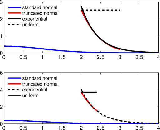
Figure 3: Doubly truncated normal distribution. The top figure has $u^{-}=2$ and $u^{+}=3$ and is better approximated with the exponential distribution. The bottom figure has $u^{-}=2$ and $u^{+}=2.5$ and the uniform is more efficient.

We use Algorithms 3 and 4, along with the methods of sampling truncated Normal variables, to sample the stability matrix $\bm{M}$. We tested this algorithm on a three dimensional model with $T=100$. In this case the dimension of $\bm{M}$ is $n=D(D+1)/2=6$. Note that this MCMC algorithm still mixes well. Fig. 4 compares the posterior distributions estimated from the Component Wise Algorithm and the standard Gibbs sampler. Notice the large differences between the distributions in each case. Similar results (not shown) are obtained for the off diagonal parameters using Algorithm 4.

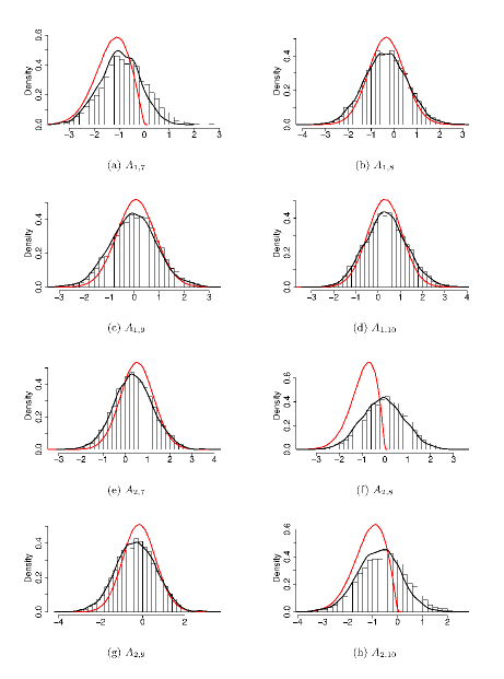
Figure 4: Estimated posterior distributions for parameters from a two dimensional model of the form Eq. 3 with N = 100 and ∆ = 0.1. The parameters, which are randomly generated, are written in the matrix notation introduced in Section 3.2.1. The histograms are the posterior distributions with uninformative prior, in red are the posterior distributions for parameters with stable SDEs and in black are the posterior distributions which include the stability matrix prior information derived in this chapter.

4 Results

4.1 Deterministic Double Well Potential Model

The first conceptual climate model we consider is a cubic model coupled to the chaotic Lorenz system (29). It is fully deterministic and consists of a slow variable which can be thought of as representing a climate process and three fast variables which can be thought of as representing chaotic weather fluctuations. The slow variable moves inside a double well potential and is perturbed by the chaotic Lorenz system, which acts effectively as noise when $\epsilon\rightarrow 0$. The equations are as follows

$$\frac{dx}{dt} = x-x^{3}+\frac{4}{90\epsilon}y_{2}$$ (27a)

$$\frac{dy_{1}}{dt} = \frac{10}{\epsilon^{2}}(y_{2}-y_{1})$$ (27b)

$$\frac{dy_{2}}{dt} = \frac{1}{\epsilon^{2}}(28y_{1}-y_{2}-y_{1}y_{3})$$ (27c)

$$\frac{dy_{3}}{dt} = \frac{1}{\epsilon^{2}}(y_{1}y_{2}-\frac{8}{3}y_{3})\,.$$ (27d)

Sample paths are displayed in Fig. 5. We now fit a one dimensional cubic SDE to the data. We just consider the general cubic form (26)

$$dX_{t}=(a_{1}+a_{2}X_{t}+a_{3}X_{t}^{2}+a_{4}X_{t}^{3})dt+\sigma dW_{t}$$ (28)

and estimate all of the parameters $\{a_{1},a_{2},a_{3},a_{4},\sigma\}$ from sparse observations of the system: again using $\Delta=10.0$ and $N=1000$. To update the drift parameters we use the Gibbs sampler of Section 3.2.1. The estimated posterior distributions are shown in Fig. 6. A lot of imputed data is needed before the estimates start to converge towards the values predicted by homogenization but the inference demonstrates that there is enough information in the sparse data set if the likelihood is well approximated.

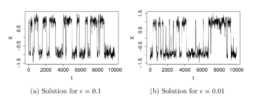
Figure 5: Example path of x of the chaotic Lorenz system: Eq. (27d)

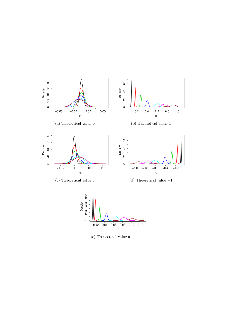
Figure 6: Posterior distribution estimates from MCMC output applied to a sparse data set ($\Delta=10$). Different distributions correspond to increasing amounts of missing data. The distribution in brown, for $m=64$, agrees with the theoretical values predicted by the homogenization procedure. In the model simulation $\epsilon=0.01$ has been used. Black line: m=1, red line: m=2, green line: m=4, blue line: m=8, light blue line: m=16, magenta line: m=32, brown line: m=64.

Figure 7 shows the predictive skill of the one dimensional reduced model for $\sigma$ estimated for various $m$. We use the empirical mean estimate for the parameter values. Figures 7a and 7b show that the reduced model can reproduce the double well distribution of the full model although the separation of each well is underestimated for $m=2$ and $m=4$ due to the larger noise. For $m\geq 8$ the model reproduces well the full models marginal distribution for $x$. It is not clear whether there is much difference between $m=8$ and $m=64$. However, observing Figures 7c and 7d we see that the autocorrelation function for the full model is much better approximated when $m=64$. This shows that the ability of our framework to impute data is a powerful way of deriving accurate reduced order models.

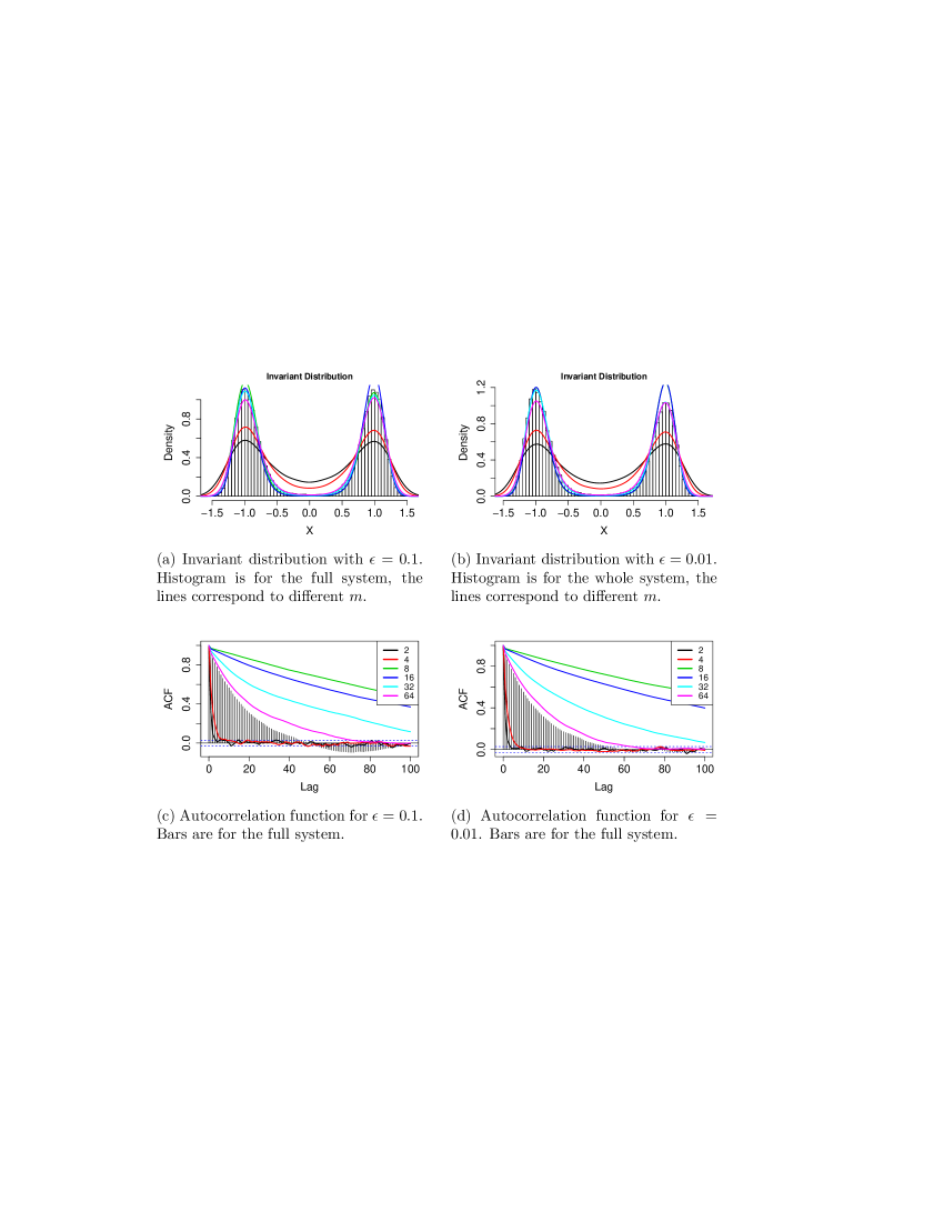
Figure 7: Predictive statistics for the reduced double well model coupled to chaotic Lorenz system: Eq. (27d) for two values of $\epsilon$. In each plot the lines correspond to the inferred one dimensional model for different $m$.

4.2 Model Reduction for Triad Systems

Now we apply our model fitting procedure to a triad model with a high dimensional deterministic system with two slow, climate variables coupled to fast chaotic dynamics. The reduction strategy has two challenges: to successfully approximate the deterministic variables by a stochastic process and to be insensitive to a lack of time scale separation.

The full system is given by

$$\frac{dx_{1}}{dt} = \frac{b_{1}}{\epsilon}x_{2}y_{1}$$ (29a)

$$\frac{dx_{2}}{dt} = \frac{b_{2}}{\epsilon}x_{1}y_{1}$$ (29b)

$$\frac{dy_{k}}{dt} = \frac{b_{3}}{\epsilon}x_{1}x_{2}\delta_{1,k}-\mbox{Re}\frac{ik}{2\epsilon^{2}}\sum_{p+q+k=0}\hat{u}_{p}^{*}\hat{u}_{q}^{*}$$ (29c)

$$\frac{dz_{k}}{dt} = -\mbox{Im}\frac{ik}{2\epsilon^{2}}\sum_{p+q+k=0}\hat{u}_{p}^{*}\hat{u}_{q}^{*},$$ (29d)

where $u_{k}=y_{k}+iz_{k}$. This system is stable provided that the energy is conserved: $b_{1}+b_{2}+b_{3}=0$. We use the values $\bm{b}=\{0.9,-0.5-0.4\}$ (our results are insensitive over a wide range of parameter values) and we choose a cut off of $\Lambda=50$. Sample paths are displayed in Fig. 8. We are interested in eliminating $\bm{y}$ leaving equations for just $x_{1}$ and $x_{2}$. The small parameter $\epsilon$ represents the time scales within the system. The variables $\bm{y}$ have fastest time scale of order $O(1/\epsilon^{2})$ compared to $O(1/\epsilon)$ for $x_{1}$ and $x_{2}$. As $\epsilon\rightarrow 0$ we can use the method of homogenization for SDEs to eliminate the fast variables and this gives

$$dx_{1}(t) = \frac{b_{1}}{\gamma}(b_{3}x_{2}^{2}(t)+\frac{\sigma^{2}}{2\gamma}b_{2})x_{1}(t)dt+\frac{\sigma}{\gamma}b_{1}x_{2}(t)dW_{t}$$ (30a)

$$dx_{2}(t) = \frac{b_{2}}{\gamma}(b_{3}x_{1}^{2}(t)+\frac{\sigma^{2}}{2\gamma}b_{1})x_{2}(t)dt+\frac{\sigma}{\gamma}b_{2}x_{1}(t)dW_{t}\,,$$ (30b)

where unknown parameters $\sigma$ and $\gamma$ have been introduced. Here we estimate them using the Algorithms 1 and 2 from observations of the climate variables alone. For convenience we consider the inference problem where the model Eq. (30) is driven by two independent Brownian motions.

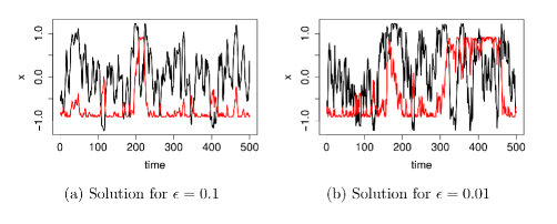
Figure 8: Example path of $x_{1}$ (black line) and $x_{2}$ (red line) from the triad model: Eq. (29)

Posterior estimates for the case $\epsilon=0.8$ are shown in Fig. 9. This value corresponds to a moderately small, though realistic (14), amount of time scale separation. As Fig. 9 demonstrates, increasing the number of imputed data leads to a convergence and, thus, to an improvement of the posterior estimates.

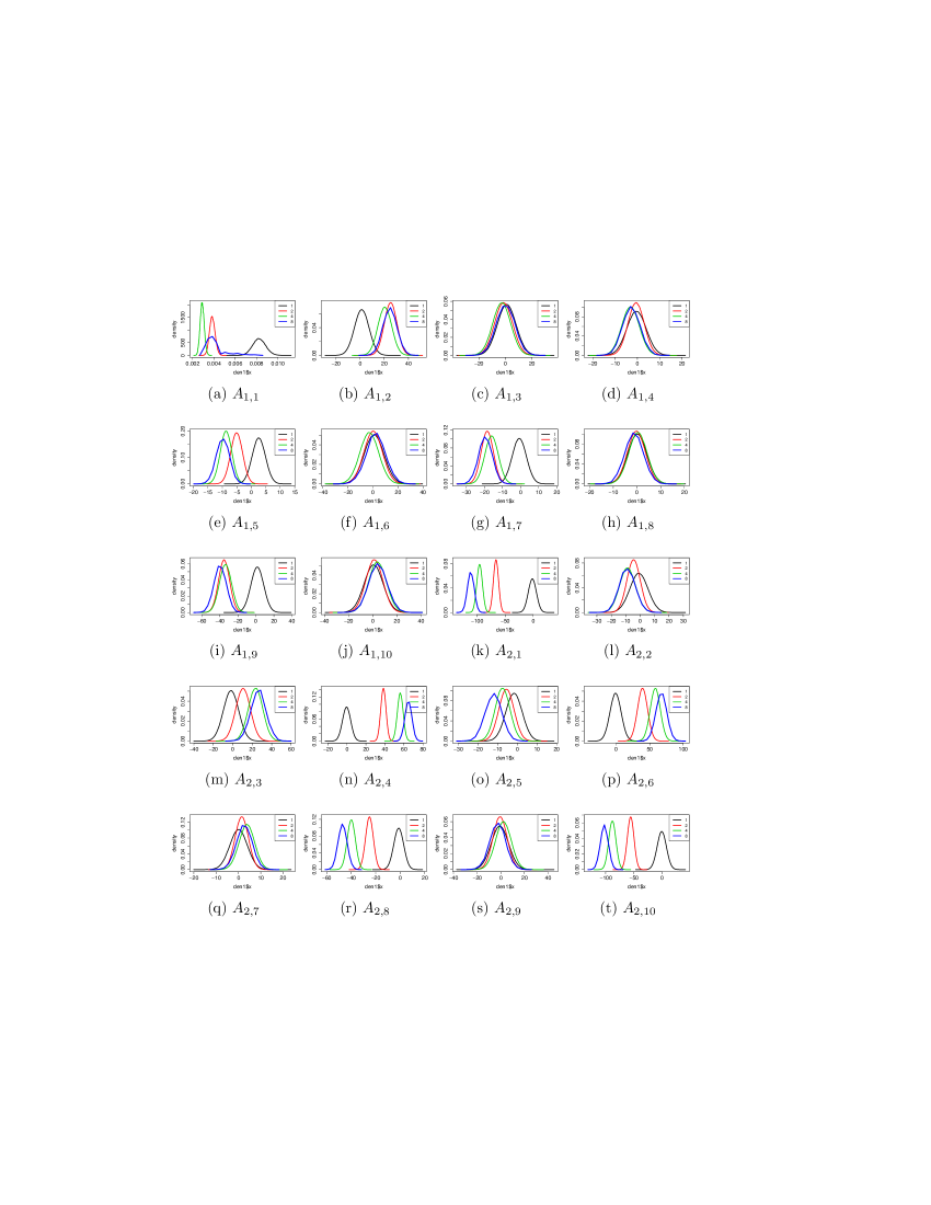
Figure 9: Posterior estimates of drift parameters for two dimensional cubic model fitted to the triad-Burgers equation for $\epsilon=0.8$.

We apply the inference to a data set with total time $T=500$ and observation interval $\Delta=0.1$. We simulate the system for $\epsilon=\{0.1,0.25,0.5,0.8,1.0\}$. Fig. 10 shows the predictive probability densities and autocorrelation functions for Eq. 30. In each case the data is simulated from the full model Eq. 29, then the parameters are estimated using the reduced model Eq. 30 and this reduced model is simulated to calculate the predictive statistics. The posterior mean estimates were computed for m = 16 missing data values (it was verified that the posteriors for m = 16 and m $<$ 16 gave consistent estimates). The reduced model Eq. 30 with empirical parameter estimates is also plotted. This model is referred to as the reduced model in Figure 10. The reduced model is able to reproduce the non-trivial shape of the PDF very well. This suggests tha reduced order models fitted from observed data can be used for extreme value studies (16).

The autocorrelation functions have been collapsed onto the reduced model by rescaling the output interval of the prediction by their value of $\epsilon$; this has been done for convenience of displaying the results. The data collapse is very good for all model simulations with the models with $\epsilon<0.5$ being closest to the reduced model. This implies that the parameter estimates for each case are partially compensating for the changing time scale separation. This provides evidence for the potential of using reduced order modelling strategies even in systems with only moderate time scale separation.

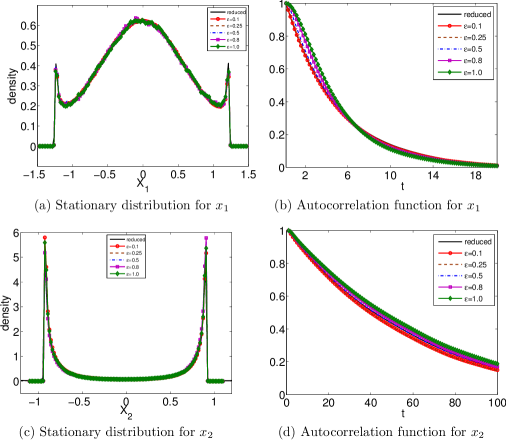
Figure 10: Output statistics comparing the reduced model Eq. 30, with empirical models for various $\epsilon$ values with the full model.

5 Summary

Here we developed a systematic Bayesian framework for the inference of the parameter of SDEs constrained by the physics of the underlying system. The physical constraints not only constrain the parameter space but also enforce global stability of the reduced order models.

For climate models we derive a constraint based on energy conservation which ensures global stability of the effective SDE. This constraint takes the form of a negative definite matrix. We then develop a new algorithm for the sampling of negative definite matrices. We also develop a new algorithm for imputing data and show that imputing data improves the accuracy considerly of the parameter estimation. We demonstrated its power successfully on two conceptual climate models.

While we focused on climate models in this study our method is general enough that it can also be applied to other areas of fluid dynamics. Furthermore, also many other physical systems observe conservation laws and, thus, stability conditions can be derived which will be useful for parameter estimation procedures.

Acknowledgments We thank three anonymous reviewers whose comments improved earlier versions of this manuscript. This study received funding from the Natural Environment Research Council, the Engineering and Physical Sciences Research Council and the Deutsche Forschungsgemeinschaft (DFG) through the cluster of excellence CliSAP.

References

- Achatz (1999) Achatz, U. and G. Branstator, A two-layer model with empirical linear corrections and reduced order for studies of internal climate variability. J. Atmos. Sci., 56, (1999) 3140-3160.
- Ait-Sahalia (2002) Ait-Sahalia, Y, Maximum likelihood estimation of discretely sampled diffusions: A closed-form approximation approach. Econometrica, 70, (2002) 223-262.
- Ait-Sahalia (2008) Ait-Sahalia, Y., Closed-form likelihood expansions for multivariate diffusions. Annals Stat., 36, (2008) 906-937.
- Barczykern and Kern (2013) Barczykern, M. and P. Kern, Representations of multidimensional linear process bridges. Rand. Oper. Stoch. Eq., 21, 159-189, (2013).
- Beskos and Roberts (2005) Beskos, A. and G. O. Roberts, Exact simulation of diffusions. Ann. Appl. Prob., 15, 2422-2444, (2005).
- Beskos et al. (2008) Beskos, A., O. Papaspiliopoulos and G. O. Roberts, A factorisation of diffusion measure and finite sample path constructions. Meth. Comp. Appl. Prob., 10, 85-104, (2008).
- Chib et al. (2004) Chib, S., Pitt, M. and Shephard, N., Likelihood based inference for diffusion driven state space models. Working Paper, Nuffield College, Oxford University, (2004).
- Crommelin and Vanden-Eijnden (2006) Crommelin, D. and E. Vanden-Eijnden, Reconstruction of diffusions using spectral data from timeseries. Comm. Math. Sci., 4 (2006), 651-668.
- Dargatz (2010) Dargatz, C., Bayesian Inference for Diffusion Processes with Applications in Life Sciences. PhD thesis, Fakultät der Mathematik, Informatik und Statistik der Ludwig Maximilians Universität München, (2010).
- Durham and Gallant (2002) Durham, G. B. and Gallant, A. R., Numerical techniques for maximum likelihood estimation of continuous-time diffusion processes. J. Bus. Econ. Statist., 20 (2002), 297-316.
- Eaton (2007) Eaton, M. L., Multivariate Statistics: A Vector Space Approach. Lecture Notes–Monograph. Series, Volume 53.
- Eraker (2001) Eraker, B., MCMC analysis of diffusion models with application to finance. J. Bus. Econ. Statist., 19 (2001), 177-191.
- Elerian (1999) Elerian, O. S., Simulation estimation of continuous-time models with applications to finance. PhD thesis, Nuffield College, Oxford (1999).
- Franzke et al. (2005) Franzke, C., A. J. Majda and E. Vanden-Eijnden, Low-Order Stochastic Mode Reduction for a Realistic Barotropic Model Climate. J. Atmos. Sci., 62 (2005), 1722-1745.
- Franzke and Majda (2006) Franzke, C., and A. J. Majda, Low-Order Stochastic Mode Reduction for a Prototype Atmospheric GCM. J. Atmos. Sci., 63 (2006), 457-479.
- Franzke (2012) Franzke, C., Predictability of Extreme Events in a Nonlinear Stochastic-Dynamical Model. Phys. Rev. E, 85 (2012), DOI: 10.1103/PhysRevE.85.031134
- Friedrich et al. (2000) Friedrich, R., S. Siegert, J. Peinke, St. Lück, M. Siefert, M. Lindemann, J. Raethjen, G. Deuschl and G. Pfister, Extracting model equations from experimental data. Phys. Lett. A, 271 (2000), 217-222.
- Golightly and Wilkinson (2008) Golightly, A. and D. J. Wilkinson, Bayesian inference for nonlinear multivariate diffusion models observed with error. Comp. Stat. Data Anal., 52 (2008), 1674-1693.
- Harlim et al. (2014) Harlim, J., A. Mahdi and A. J. Majda, An ensemble Kalman filter for statistical estimation of physics constrained nonlinear regression models. J. Comp. Phys., 257, (2014), 782-812.
- Heinz (2003) Heinz, S., Statiscal mechanics of turbulent flows. Springer Verlag Berlin, (2014), 240pp.
- Horenko et al. (2005) Horenko, I., E. Dittmer and C. Schütte, Reduced stochastic models for complex molecular systems. SIAM Comp. Vis. Sci., 9, (2005), 789-102.
- Kondrashov et al. (2006) Kondrashov, D., S. Kravtsov and M. Ghil, Empirical mode reduction in a model of extratropical low-frequency variability. J. Atmos. Sci., 63 (2006), 1859-1877.
- Majda et al. (1999) Majda, A. J., I. Timofeyev and E. Vanden-Eijnden, Models for stochastic climate prediction. Proc. Nat. Acad. Sci. USA, 96 (1999), 14687-14691.
- Majda et al. (2001) Majda, A. J., I. Timofeyev and E. Vanden-Eijnden, A mathematical framework for stochastic climate models. Commun. Pure Appl. Math., 54 (2001), 891-974.
- Majda et al. (2008) Majda, A. J., C. Franzke and B. Khouider, An applied mathematics perspective on stochastic modelling for climate. Phil. Trans. R. Soc. A, 366 (2008), 2429-2455.
- Majda et al. (2009) Majda, A. J., C. Franzke and D. Crommelin, Normal forms for reduced stochastic climate models. Proc. Nat. Acad. Sci. USA, 106, (2009) 3649-3653. doi: 10.1073/pnas.0900173106
- Majda and Yuan (2012) Majda, A. J. and Y. Yuan, Fundamental limitations of ad hoc linear and quadratic multi-level regression models for physical systems. Disc. Con. Dyn. Sys., 17, (2012) 1333-1363.
- Majda and Harlim (2013) Majda, A. J. and J. Harlim, Physics constrained nonlinear regression models for time series. Nonlinearity, 26, (2013) 201-217.
- Mitchell and Gottwald (2012) Mitchell, L. and Gottwald, G. A., Data Assimilation in Slow-Fast Systems Using Homogenized Climate Models. J. Atmos. Sci., 69, (2012) 1359-1377.
- Ozaki (1992) Ozaki, T., A bridge between nonlinear time series models and nonlinear stochastic dynamic systems. A local linearization approach. Stat. Sinica, 2, (1992) 113-135.
- Pavliotis and Stuart (2008) Pavliotis, G. A. and A. M. Stuart, Multiscale methods, Springer Verlag, (2008) 310pp.
- Peavoy (2013) Peavoy, D., Methods of likelihood based inference for constructing stochastic climate models, PhD thesis, University of Warwick, (2013) 232pp.
- Pedersen (1995) Pedersen, A. R., A new approach to maximum likelihood estimation for stochastic differential equations based on discrete observations. Scand. J. Statist., 22, (1995) 55-71.
- Robert (1995) Robert, C., Simulation of truncated normal variables. Stat. Comp., 5, (1995) 121-125.
- Roberts et al. (1997) Roberts, G. O., A. Gelman and W. R. Gilks, Weak convergence and optimal scaling of random walk Metropolis algorithms. Ann. App. Prob., 7, (1997) 110-120.
- Roberts and Stramer (2001) Roberts, G. O. and Stramer, O., On inference for partially observed nonlinear diffusion models using the Metropolis-Hastings algorithm. Biometrika, 88, (2001) 603-621.
- Selten (1995) Selten, F. M., An efficient description of the dynamics of barotropic flow. J. Atmos. Sci., 52, (1995) 915-936.
- Shephard and Pitt (1997) Shephard, N. and Pitt, M. K., Likelihood analysis of non-Gaussian measurement time series. Biometrika, 84, (1997) 653-667.
- Shoji and Ozaki (1998) Shoji, I. and T. Ozaki, Estimation for nonlinear stochastic differential equations by a local linearization method. Stoch. Anal. Appl., 16, (1998) 733-752.
- Siegert et al. (1998) Siegert, S., R. Friedrich and J. Peinke, Analysis of data sets of stochastic systems. Phys. Lett. A, 243 (1998), 275-280.
- Yuan and Majda (2011) Yuan, Y. and A. J. Majda, Invariant measures and asymptodic Gaussian bounds for normal forms of stochastic climate models. Chin. Ann. Math., 32 (2011), 343-368.