Travel time estimation for ambulances using Bayesian data augmentation

Abstract

We introduce a Bayesian model for estimating the distribution of ambulance travel times on each road segment in a city, using Global Positioning System (GPS) data. Due to sparseness and error in the GPS data, the exact ambulance paths and travel times on each road segment are unknown. We simultaneously estimate the paths, travel times, and parameters of each road segment travel time distribution using Bayesian data augmentation. To draw ambulance path samples, we use a novel reversible jump Metropolis–Hastings step. We also introduce two simpler estimation methods based on GPS speed data.

We compare these methods to a recently published travel time estimation method, using simulated data and data from Toronto EMS. In both cases, out-of-sample point and interval estimates of ambulance trip times from the Bayesian method outperform estimates from the alternative methods. We also construct probability-of-coverage maps for ambulances. The Bayesian method gives more realistic maps than the recently published method. Finally, path estimates from the Bayesian method interpolate well between sparsely recorded GPS readings and are robust to GPS location errors.

T1Supported in part by NSF Grant CMMI-0926814 and NSF Grant DMS-12-09103.

, , and

1 Introduction

Emergency medical service (EMS) providers prefer to assign the closest available ambulance to respond to a new emergency [Dean (2008)]. Thus, it is vital to have accurate estimates of the travel time of each ambulance to the emergency location. An ambulance is often assigned to a new emergency while away from its base [Dean (2008)], so the problem is more difficult than estimating response times from several fixed bases. Travel times also play a central role in positioning bases and parking locations [Brotcorne, Laporte and Semet (2003), Goldberg (2004), Henderson (2010)]. Accounting for variability in travel times can lead to considerable improvements in EMS management [Erkut, Ingolfsson and Erdoğan (2008), Ingolfsson, Budge and Erkut (2008)]. We introduce methods for estimating the distribution of travel times for arbitrary routes on a municipal road network using historical trip durations and vehicle Global Positioning System (GPS) readings. This enables estimation of fastest paths in expectation between any two locations, as well as estimation of the probability an ambulance will reach its destination within a given time threshold.

Most EMS providers record ambulance GPS information; we use data from Toronto EMS from 2007–2008. The GPS data include locations, timestamps, speeds, and vehicle and emergency incident identifiers. Readings are stored every 200 meters (m) or 240 seconds (s), whichever comes first. The true sampling rate is higher, but this scheme minimizes data transmission and storage. This is standard practice across EMS providers, though the storage rates vary [Mason (2005)]. In related applications the GPS readings can be even sparser; Lou et al. (2009) analyzed data from taxis in Tokyo in which GPS readings are separated by 1–2 km or more.

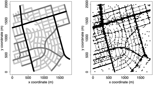
Figure 1: Left: A subregion of Toronto, with primary roads (black), secondary roads (gray) and tertiary roads (light gray). Right: GPS data on this region from the Toronto EMS lights-and-sirens data set.

The GPS location and speed data are also subject to error. Location accuracy degrades in urban canyons, where GPS satellites may be obscured and signals reflected [Chen et al. (2005), Mason (2005), Syed (2005)]. Chen et al. (2005) observed average location errors of 27 m in parts of Hong Kong with narrow streets and tall buildings, with some errors over 100 m. Location error is also present in the Toronto data; see Figure 1. Witte and Wilson (2004) found GPS speed errors of roughly 5% on average, with largest error at high speeds and when few GPS satellites were visible.

Recent work on estimating ambulance travel time distributions has been done by Budge, Ingolfsson and Zerom (2010) and Aladdini (2010) using estimates based on total trip distance and time, not GPS data. Budge et al. proposed modeling the log travel times using a $t$-distribution, where the median and coefficient of variation are functions of the trip distance (see Section 4.2). Aladdini found that the lognormal distribution provided a good fit for ambulance travel times between specific start and end locations. Budge et al. found heavier tails than Aladdini, in part because they did not condition on the trip location. Neither of these papers considered travel times on individual road segments. For this reason they cannot capture some desired features, such as faster response times to locations near major roads.

We first introduce two local methods using only the GPS locations and speeds (Section 4.1). Each GPS reading is mapped to the nearest road segment (the section of road between neighboring intersections), and the mapped speeds are used to estimate the travel time for each segment. In the first method, we use the harmonic mean of the mapped GPS speeds to create a point estimator of the travel time. We are the first to propose this estimator for mapped GPS data, though it is commonly used for estimating travel times via speed data recorded by loop detectors [Rakha and Zhang (2005), Soriguera and Robuste (2011), Wardrop (1952)]. We give theoretical results supporting this approach in the supplementary material [Westgate et al. (2013)]. This method also yields interval and distribution estimates of the travel time. In our second local method, we assume a parametric distribution for the GPS speeds on each segment and calculate maximum likelihood estimates of the parameters of this distribution. These can be used to obtain point, interval, or distribution estimates of the travel time.

In Sections 2 and 3, we propose a more sophisticated method, modeling the data at the trip level. Whereas the local methods use only GPS data and the method of Budge et al. uses only the trip start and end locations and times, this method combines the two sources of information. We simultaneously estimate the path driven for each ambulance trip and the distribution of travel times on each road segment using Bayesian data augmentation [Tanner and Wong (1987)]. For computation, we introduce a reversible jump Markov chain Monte Carlo method [Green (1995)]. Although parameter estimation is more computationally intensive than for the other methods, prediction is very fast. Also, the parameter estimates are updated offline, so the increased computation time is not an operational handicap.

We compare the predictive accuracy on out-of-sample trips for the Bayesian method, the local methods, and the method of Budge et al. on a subregion of Toronto, using simulated data and real data (Sections 6 and 7). Since the methods have some bias due in part to the GPS sampling scheme, we first use a correction factor to make each method approximately unbiased (Section 5). On simulated data, point estimates from the Bayesian method outperform the alternative methods by over 50% in root mean squared error, relative to an Oracle method with the lowest possible error. On real data, point estimates from the Bayesian method again outperform the alternative methods. Interval estimates from the Bayesian method have dramatically better coverage than intervals from the local methods.

We also produce probability-of-coverage maps [Budge, Ingolfsson and Zerom (2010)], showing the probability of traveling from a given intersection to any other intersection within a time threshold (Section 7.4). This is the performance standard in many EMS contracts; an EMS organization attempts to respond to, for example, 90% of all emergencies within 9 minutes [Fitch (1995)]. The estimates from the Bayesian method are more realistic than those of Budge et al., because they differentiate between equidistant locations based on whether or not they can be reached by fast roads.

Finally, we assess the ambulance path estimates from the Bayesian method (Sections 6.3 and 7.5). Estimating the path driven from a discrete set of GPS readings is called the map-matching problem [Mason (2005)]. Most map-matching algorithms return a single path estimate [Krumm, Letchner and Horvitz (2007), Lou et al. (2009), Marchal, Hackney and Axhausen (2005), Mason (2005)]. However, our posterior distribution can capture multiple high-probability paths when the true path is unclear from the GPS data. Our path estimates interpolate accurately between widely-separated GPS locations and are robust to GPS error.

2 Bayesian formulation

2.1 Model

Consider a network of $J$ directed road segments, called arcs, and a set of $I$ ambulance trips on this network. Assume that each trip starts and finishes on known nodes (intersections) $d_{i}^{s}$ and $d_{i}^{f}$ in the network, at known times $t_{i}^{s}$ and $t_{i}^{f}$. Therefore, the total travel time $t_{i}^{f}-t_{i}^{s}$ is known. In practice, trips sometimes begin or end in the interior of a road segment, however, road segments are short enough that this is a minor issue. The median road segment length in the full Toronto network is 111 m, the mean is 162 m, and the maximum is 4613 m. Each trip $i$ has observed GPS readings, indexed by $\ell\in\{1,\ldots,r_{i}\}$, and gathered at known times $t_{i}^{\ell}$. GPS reading $\ell$ is the triplet $(X_{i}^{\ell},Y_{i}^{\ell},V_{i}^{\ell})$, where $X_{i}^{\ell}$ and $Y_{i}^{\ell}$ are the measured geographic coordinates and $V_{i}^{\ell}$ is the measured speed. Denote $G_{i}=\{(X_{i}^{\ell},Y_{i}^{\ell},V_{i}^{\ell})\}_{\ell=1}^{r_{i}}$.

The relevant unobserved variables for each trip $i$ are the following: [1.]

The unknown path (sequence of arcs) $A_{i}=\{A_{i,1},\ldots,A_{i,N_{i}}\}$ traveled by the ambulance from $d_{i}^{s}$ to $d_{i}^{f}$. The path length $N_{i}$ is also unknown.

The unknown travel times $T_{i}=(T_{i,1},\ldots,T_{i,N_{i}})$ on the arcs in the path. We use the notation $T_{i}(j)$ to refer to the travel time in trip $i$ on arc $j$.

We model the observed and unobserved variables $\{A_{i},T_{i},G_{i}\}_{i=1}^{I}$ as follows. Conditional on $A_{i}$, each element $T_{i,k}$ of the vector $T_{i}$ follows a lognormal distribution with parameters $\mu_{A_{i,k}},\sigma^{2}_{A_{i,k}}$, independently across $i$ and $k$. We use the notation $T_{i,k}|A_{i}\sim\mathcal{LN}(\mu_{A_{i,k}},\sigma^{2}_{A_{i,k}})$. In the literature, ambulance travel times between specific locations have been observed and modeled to be lognormal [Aladdini (2010), Alanis, Ingolfsson and Kolfal (2012)]. Denote the expected travel time on each arc $j\in\{1,\ldots,J\}$ by $\theta(j)=\exp(\mu_{j}+\sigma_{j}^{2}/2)$. We use a multinomial logit choice model [McFadden (1973)] for the path $A_{i}$, with likelihood

$$f(A_{i})=\frac{\exp(-C\sum_{k=1}^{N_{i}}\theta(A_{i,k}))}{\sum_{a_{i}\in\mathcal{P}_{i}}\exp(-C\sum_{k=1}^{n_{i}}\theta(a_{i,k}))},$$ (1)

where $C>0$ is a fixed constant, $\mathcal{P}_{i}$ is the set of possible paths with no repeated nodes from $d_{i}^{s}$ to $d_{i}^{f}$ in the network, and $a_{i}=\{a_{i,1},\ldots,a_{i,n_{i}}\}$ indexes the paths in $\mathcal{P}_{i}$. In this model, the fastest routes in expectation have the highest probability.

We assume that ambulances travel at constant speed on a single arc in a given trip. This approximation is necessary since there is typically at most one GPS reading on any arc in a given trip, and thus little information in the data regarding changes in speed on individual arcs. Therefore, the true location and speed of the ambulance at time $t_{i}^{\ell}$ are deterministic functions $\operatorname{loc}(A_{i},T_{i},t_{i}^{\ell})$ and $\operatorname{sp}(A_{i},T_{i},t_{i}^{\ell})$ of $A_{i}$ and $T_{i}$. Conditional on $A_{i},T_{i}$, the measured location $(X_{i}^{\ell},Y_{i}^{\ell})$ is assumed to have a bivariate normal distribution [a standard assumption; see Krumm, Letchner and Horvitz (2007), Mason (2005)] centered at $\operatorname{loc}(A_{i},T_{i},t_{i}^{\ell})$, with known covariance matrix $\Sigma$. Similarly, the measured speed $V_{i}^{\ell}$ is assumed to have a lognormal distribution with expectation equal to $\operatorname{sp}(A_{i},T_{i},t_{i}^{\ell})$ and variance parameter $\zeta^{2}$:

$$\bigl{(}X_{i}^{\ell},Y_{i}^{\ell}\bigr{)}\big{|}A_{i},T_{i}\sim N_{2}\bigl{(}\operatorname{loc}\bigl{(}A_{i},T_{i},t_{i}^{\ell}\bigr{)},\Sigma\bigr{)},$$ (2)

$$\displaystyle\log V_{i}^{\ell}\Big{|}A_{i},T_{i}\sim N\biggl{(}\log\operatorname{sp}\bigl{(}A_{i},T_{i},t_{i}^{\ell}\bigr{)}-\frac{\zeta^{2}}{2},\zeta^{2}\biggr{)}.$$ (3)

We assume independence between all the GPS speed and location errors. Combining equations (1)–(3), we obtain the likelihood

$$f\bigl{(}\{A_{i},T_{i},G_{i}\}_{i=1}^{I}\big{|}\bigl{\{}\mu_{j},\sigma_{j}^{2}\bigr{\}}_{j=1}^{J},\zeta^{2}\bigr{)}$$

$$\qquad=\prod_{i=1}^{I}\Biggl{[}f(A_{i})\prod_{k=1}^{N_{i}}\mathcal{LN}\bigl{(}T_{i,k};\mu_{A_{i,k}},\sigma^{2}_{A_{i,k}}\bigr{)}$$

(4)

$$\hskip 51.0pt{}\times\prod_{\ell=1}^{r_{i}}\biggl{[}N_{2}\bigl{(}\bigl{(}X_{i}^{\ell},Y_{i}^{\ell}\bigr{)};\operatorname{loc}\bigl{(}A_{i},T_{i},t_{i}^{\ell}\bigr{)},\Sigma\bigr{)}$$

$$\hskip 82.0pt{}\times\mathcal{LN}\biggl{(}V_{i}^{\ell};\log\operatorname{sp}\bigl{(}A_{i},T_{i},t_{i}^{\ell}\bigr{)}-\frac{\zeta^{2}}{2},\zeta^{2}\biggr{)}\biggr{]}\Biggr{]}.$$

In practice, we use data-based choices for the constants $\Sigma$ and $C$ (see the supplementary material [Westgate et al. (2013)]). The unknown parameters in the model are the arc travel time parameters $\{\mu_{j},\sigma_{j}^{2}\}_{j=1}^{J}$ and the GPS speed error parameter $\zeta^{2}$.

2.2 Prior distributions

To complete the model, we specify independent prior distributions for the unknown parameters. We use $\mu_{j}\sim N(m_{j},s^{2})$, $\sigma_{j}\sim\operatorname{Unif}(b_{1},b_{2})$, and $\zeta\sim\operatorname{Unif}(b_{3},b_{4})$, where $m_{j}$, $s^{2}$, $b_{1}$, $b_{2}$, $b_{3}$, $b_{4}$ are fixed hyperparameters. A normal prior is a standard choice for the location parameter of a lognormal distribution. We use uniform priors on the standard deviations $\sigma_{j}$ and $\zeta$ [Gelman (2006)]. The prior ranges $[b_{1},b_{2}]$ and $[b_{3},b_{4}]$ are made wide enough to capture all plausible parameter values. The prior mean for $\mu_{j}$ depends on $j$, because there are often existing road speed estimates that can be used to specify $m_{j}$. Prior information regarding the values $s^{2}$, $b_{1}$, $b_{2}$, $b_{3}$, $b_{4}$ is more limited. We use a combination of prior information and the data to specify all hyperparameters, as described in the supplementary material [Westgate et al. (2013)].

3 Bayesian computational method

We use a Markov chain Monte Carlo method to obtain samples $(\zeta^{2(\ell)},\{\mu_{j}^{(\ell)},\sigma_{j}^{(\ell)}\}_{j=1}^{J},\{A_{i}^{(\ell)},T_{i}^{(\ell)}\}_{i=1}^{I})$ from the joint posterior distribution of all unknowns [Robert and Casella (2004), Tierney (1994)]. Each unknown quantity is updated in turn, conditional on the other unknowns, via either a draw from the closed-form conditional posterior distribution or a Metropolis–Hastings (M–H) move. Estimation of any desired function $g(\zeta^{2},\{\mu_{j},\sigma_{j}^{2}\}_{j=1}^{J})$ of the unknown parameters is done via Monte Carlo, taking $\hat{g}=\frac{1}{M}\sum_{\ell=1}^{M}g(\zeta^{2(\ell)},\{\mu_{j}^{(\ell)},\sigma_{j}^{2(\ell)}\}_{j=1}^{J}).$

3.1 Markov chain initial conditions

To initialize each path $A_{i}$, select the middle GPS reading, reading number $\lfloor r_{i}/2\rfloor+1$. Find the nearest node in the road network to this GPS location, and route the initial path $A_{i}$ through this node, taking the shortest-distance path to and from the middle node. To initialize the travel time vector $T_{i}$, distribute the known trip time across the arcs in the path $A_{i}$, weighted by arc length. Finally, to initialize $\zeta^{2}$ and each $\mu_{j}$ and $\sigma^{2}_{j}$, draw from their priors.

3.2 Updating the paths

Updating the path $A_{i}$ may also require updating the travel times $T_{i}$, since the number of arcs in the path may change. Since this changes the dimension of the vector $T_{i}$, we update $(A_{i},T_{i})$ using a reversible jump M–H move [Green (1995)]. Calling the current values $(A_{i}^{(1)},T_{i}^{(1)})$, we propose new values $(A_{i}^{(2)},T_{i}^{(2)})$ and accept them with the appropriate probability, detailed below.

The proposal changes a contiguous subset of the path. The length (number of arcs) of this subpath is limited to some maximum value $K$; we specify $K$ in Section 3.5. Precisely: [3.]

With equal probability, choose a node $d^{\prime}$ from the path $A_{i}^{(1)}$, excluding the final node.

Let $a^{(1)}$ be the number of nodes that follow $d^{\prime}$ in the path. With equal probability, choose an integer $w\in\{1,\ldots,\min(a^{(1)},K)\}$. Denote the $w$th node following $d^{\prime}$ as $d^{\prime\prime}$. The subpath from $d^{\prime}$ to $d^{\prime\prime}$ is the section to be updated (the “current update section”).

Consider all possible routes of length up to $K$ from $d^{\prime}$ to $d^{\prime\prime}$. With equal probability, propose one of these routes as a change to the path (the “proposed update section”), giving the proposed path $A_{i}^{(2)}$.

Next we propose travel times $T^{(2)}_{i}$ that are compatible with $A_{i}^{(2)}$. Let $\{c_{1},\ldots,c_{m}\}\subset A_{i}^{(1)}$ and $\{p_{1},\ldots,p_{n}\}\subset A_{i}^{(2)}$ denote the arcs in the current and proposed update sections, noting that $m$ and $n$ may be different. Recall that $T_{i}(j)$ denotes the travel time of trip $i$ on arc $j$. For each arc $j\in A_{i}^{(2)}\setminus\{p_{1},\ldots,p_{n}\}$, set $T^{(2)}_{i}(j)=T_{i}^{(1)}(j)$. Let $S_{i}=\sum_{\ell=1}^{m}T_{i}^{(1)}(c_{\ell})$ be the total travel time of the current update section. Since the total travel time of the entire trip is known (see Section 2.1), $S_{i}$ is fixed and known as well, conditional on the travel times for the arcs that are unchanged by this update. Therefore, we must have $\sum_{\ell=1}^{n}T^{(2)}_{i}(p_{\ell})=S_{i}$. The travel times $T^{(2)}_{i}(p_{1}),\ldots,T^{(2)}_{i}(p_{n})$ are proposed by drawing $(r_{1},\ldots,r_{n})\sim\operatorname{Dirichlet}(\alpha\theta(p_{1}),\ldots,\alpha\theta(p_{n}))$ for a constant $\alpha>0$ (specified below), and setting $T^{(2)}_{i}(p_{\ell})=r_{\ell}S_{i}$ for $\ell\in\{1,\ldots,n\}$. The expected value of the proposed travel time on arc $p_{\ell}$ is $E(T^{(2)}_{i}(p_{\ell}))=S_{i}\frac{\theta(p_{\ell})}{\sum_{k=1}^{n}\theta(p_{k})}$. Therefore, the expected values of the proposed times are weighted by the arc travel time expected values [Gelman et al. (2004)]. The constant $\alpha$ controls the variances and covariances of the components $T_{i}^{(2)}(p_{\ell})$. In our experience $\alpha=1$ works well; one can also tune $\alpha$ to obtain a desired acceptance rate for a particular data set [Robert and Casella (2004), Roberts and Rosenthal (2001)].

Let $N_{i}^{(j)}$ be the number of edges in the path $A_{i}^{(j)}$ for $j\in\{1,2\}$, and let $a^{(2)}$ be the number of nodes that follow $d^{\prime}$ in the path $A_{i}^{(2)}$. We accept the proposal $(A^{(2)}_{i},T_{i}^{(2)})$ with probability equal to the minimum of one and

$$\frac{f_{i}(A^{(2)}_{i},T^{(2)}_{i},G_{i}|\{\mu_{j},\sigma^{2}_{j}\}_{j=1}^{J},\zeta^{2})}{f_{i}(A_{i}^{(1)},T_{i}^{(1)},G_{i}|\{\mu_{j},\sigma^{2}_{j}\}_{j=1}^{J},\zeta^{2})}\times\frac{N_{i}^{(1)}\min(a^{(1)},K)}{N^{(2)}_{i}\min(a^{(2)},K)}$$

(5)

$$\qquad\times\frac{\operatorname{Dir}({T_{i}^{(1)}(c_{1})}/{S_{i}},\ldots,{T_{i}^{(1)}(c_{m})}/{S_{i}};\alpha\theta(c_{1}),\ldots,\alpha\theta(c_{m}))}{\operatorname{Dir}({T_{i}^{(2)}(p_{1})}/{S_{i}},\ldots,{T_{i}^{(2)}(p_{n})}/{S_{i}};\alpha\theta(p_{1}),\ldots,\alpha\theta(p_{n}))}S_{i}^{n-m},$$

where $f_{i}$ is the contribution of trip $i$ to equation (2.1) and $\operatorname{Dir}(x;y)$ denotes the Dirichlet density with parameter vector $y$, evaluated at $x$. The proposal density for the travel times $T^{(2)}_{i}(p_{1}),\ldots,T^{(2)}_{i}(p_{n})$ requires a change of variables from the Dirichlet density. This leads to the factor $S_{i}^{n-m}$ in the ratio of proposal densities. In the supplementary material [Westgate et al. (2013)], we show that this move is valid since it is reversible with respect to the conditional posterior distribution of $(A_{i},T_{i})$.

3.3 Updating the trip travel times

To update the realized travel time vector $T_{i}(j)$, we use the following M–H move. Given current travel times $T_{i}^{(1)}$, we propose travel times $T_{i}^{(2)}$: [2.]

With equal probability, choose a pair of distinct arcs $j_{1}$ and $j_{2}$ in the path $A_{i}$. Let $S_{i}=T^{(1)}_{i}(j_{1})+T^{(1)}_{i}(j_{2})$.

Draw $(r_{1},r_{2})\sim\operatorname{Dirichlet}(\alpha^{\prime}\theta(j_{1}),\alpha^{\prime}\theta(j_{2}))$. Set $T^{(2)}_{i}(j_{1})=r_{1}S_{i}$ and$T^{(2)}_{i}(j_{2})=r_{2}S_{i}$. Similarly to the path proposal above, this proposal randomly distributes the travel time over the two arcs, weighted by the expected travel times $\theta(j_{1})$ and $\theta(j_{2})$, with variances controlled by the constant $\alpha^{\prime}$ [Gelman et al. (2004)]. In our experience $\alpha^{\prime}=0.5$ is effective for our application. It is straightforward to calculate the M–H acceptance probability.

3.4 Updating the parameters $\mu_{j}$, $\sigma_{j}^{2}$, and $\zeta^{2}$

To update each $\mu_{j}$, we sample from the full conditional posterior distribution, which is available in closed form. We have $\mu_{j}|\sigma^{2}_{j},\{A_{i},T_{i}\}_{i=1}^{I}\sim N(\hat{\mu}_{j},\hat{s}^{2}_{j})$, where

$$\hat{s}^{2}_{j}=\biggl{[}\frac{1}{s^{2}}+\frac{n_{j}}{\sigma^{2}_{j}}\biggr{]}^{-1},\qquad\hat{\mu}_{j}=\hat{s}^{2}_{j}\biggl{[}\frac{m_{j}}{s^{2}}+\frac{1}{\sigma^{2}_{j}}\sum_{i\in I_{j}}\log T_{i}(j)\biggr{]},$$

the set $I_{j}\subset\{1,\ldots,I\}$ indicates the subset of trips using arc $j$, and $n_{j}=|I_{j}|$.

To update each $\sigma^{2}_{j}$, we use a local M–H step [Tierney (1994)]. We propose $\sigma_{j}^{2*}\sim\mathcal{LN}(\log\sigma_{j}^{2},\eta^{2})$, having fixed variance $\eta^{2}$. The M–H acceptance probability $p_{\sigma}$ is the minimum of 1 and

$$\frac{\sigma_{j}}{\sigma^{*}_{j}}\mathbf{1}_{\{\sigma^{*}_{j}\in[b_{1},b_{2}]\}}\biggl{(}\frac{\prod_{i\in I_{j}}\mathcal{LN}(T_{i}(j);\mu_{j},\sigma^{2*}_{j})}{\prod_{i\in I_{j}}\mathcal{LN}(T_{i}(j);\mu_{j},\sigma^{2}_{j})}\biggr{)}\frac{\mathcal{LN}(\sigma^{2}_{j};\log(\sigma^{2*}_{j}),\eta^{2})}{\mathcal{LN}(\sigma^{2*}_{j};\log(\sigma^{2}_{j}),\eta^{2})}.$$

To update $\zeta^{2}$, we use another M–H step with a lognormal proposal, with variance $\nu^{2}$. The proposal variances $\eta^{2},\nu^{2}$ are tuned to achieve an acceptance rate of approximately 23% [Roberts and Rosenthal (2001)].

3.5 Markov chain convergence

The transition kernel for updating the path $A_{i}$ is irreducible, and hence valid [Tierney (1994)], if it is possible to move between any two paths in $\mathcal{P}_{i}$ in a finite number of iterations, for all $i$. For a given road network, the maximum update section length $K$ can be set high enough to meet this criterion. However, the value of $K$ should be set as low as possible, because increasing $K$ tends to lower the acceptance rate. If there is a region of the city with sparse connectivity, the required value of $K$ may be impractically large. For example, there could be a single arc of a highway alongside many arcs of a parallel minor road. Then, a large $K$ would be needed to allow transitions between the highway and the minor road. If $K$ is kept smaller, the Markov chain is reducible. In this case, the chain converges to the posterior distribution restricted to the closed communicating class in which the chain is absorbed. If this class contains much of the posterior mass, as might arise if the initial path follows the GPS data reasonably closely, then this should be a good approximation.

In Sections 6 and 7, we apply the Bayesian method to simulated data and data from Toronto EMS, on a subregion of Toronto with 623 arcs. Each Markov chain was run for 50,000 iterations (where each iteration updates all parameters), after a burn-in period of 25,000 iterations. We calculated Gelman–Rubin diagnostics [Gelman and Rubin (1992)], using two chains, for the parameters $\zeta^{2}$, $\mu_{j}$, and $\sigma^{2}_{j}$. Results from a typical simulation study were as follows: potential scale reduction factor of 1.06 for $\zeta^{2}$, of less than 1.1 for $\mu_{j}$ for 549 arcs (88.1%), between 1.1–1.2 for 43 arcs (6.9%), between 1.2–1.5 for 30 arcs (4.8%), and less than 2 for the remaining 1 arc, with similar results for the parameters $\sigma^{2}_{j}$. These results indicate no lack of convergence.

Each Markov chain run for these experiments takes roughly 2 hours on a 3.2 GHz workstation. Each iteration of the Markov chain scales linearly in time with the number of arcs and the number of ambulance trips: $O(J+I)$, assuming the lengths of the ambulance paths do not grow as well. This assumption is reasonable, since long ambulance paths are undesirable for an EMS provider. It is much more difficult to assess how the number of iterations required for convergence changes with $J$ and $I$, since this would require bounding the spectral gap of the Markov chain. The full Toronto road network has roughly 110 times as many arcs as the test region, and the full Toronto EMS data set has roughly 80 times as many ambulance trips.

In practice, parameter estimates are updated infrequently and offline. Once parameter estimation is done, prediction for new routes and generation of our figures is very fast. If parameter estimation for the Bayesian method is computationally impractical for the entire city, it can be divided into multiple regions and estimated in parallel. We envision creating overlapping regions and discarding estimates on the boundary to eliminate edge effects (see Section 7.1). During parameter estimation, trips traveling through multiple regions would be divided into portions for each region, as we have done in our Toronto EMS experiments. However, prediction for such a trip can be handled directly, given the parameter estimates for all arcs in the city. The fastest path in expectation may be calculated using a shortest path algorithm over the entire road network, which gives a point estimate of the trip travel time. A distribution estimate of the travel time can be obtained by sampling travel times on the arcs in this fastest path (see Section 7.3).

4 Comparison methods

4.1 Local methods

Here we detail the two local methods outlined in Section 1. Each GPS reading is mapped to the nearest arc (both directions of travel are treated together). Let $n_{j}$ be the number of GPS points mapped to arc $j$, $L_{j}$ the length of arc $j$, and $\{V_{j}^{k}\}_{k=1}^{n_{j}}$ the mapped speed observations. We assume constant speed on each arc, as in the Bayesian method. Thus, let $T_{j}^{k}=L_{j}/V_{j}^{k}$ be the travel time associated with observed speed $V_{j}^{k}$.

In the first local method, we calculate the harmonic mean of the speeds $\{V_{j}^{k}\}_{k=1}^{n_{j}}$ and convert to a travel time point estimate

$$\hat{T}_{j}^{H}=\frac{L_{j}}{n_{j}}\sum_{k=1}^{n_{j}}\frac{1}{V^{k}_{j}}.$$

This is equivalent to calculating the arithmetic mean of the associated travel times $T_{j}^{k}$. The empirical distribution of the associated times $\{T_{j}^{k}\}_{k=1}^{n_{j}}$ can be used as a distribution estimate. Because readings with speed 0 occur in the Toronto EMS data set, we set any reading with speed below 5 miles per hour (mph) equal to 5 mph. This harmonic mean estimator is well known in the transportation research literature, where it is called the “space mean speed,” in the context of estimating travel times using speed data recorded by loop detectors [Rakha and Zhang (2005), Soriguera and Robuste (2011), Wardrop (1952)].

In the supplementary material [Westgate et al. (2013)], we consider this travel time estimator $\hat{T}_{j}^{H}$ and its relation to the GPS sampling scheme. We show that if GPS points are sampled by distance (e.g., every 100 m), $\hat{T}_{j}^{H}$ is an unbiased estimator for the true mean travel time. However, if GPS points are sampled by time (e.g., every 30 s), $\hat{T}_{j}^{H}$ overestimates the mean travel time. The Toronto EMS data set uses a combination of sampling-by-distance and sampling-by-time. However, the distance constraint is usually satisfied first (see Figure 5, where the sampled GPS points are regularly spaced). Thus, the travel time estimator $\hat{T}_{j}^{H}$ is appropriate.

In the second local method, we assume $V_{j}^{k}\sim\mathcal{LN}(m_{j},s_{j}^{2})$, independently across $k$, for unknown travel time parameters $m_{j}$ and $s_{j}^{2}$. This distribution on the travel speed implies that the travel times also have a lognormal distribution: $T_{j}^{k}\sim\mathcal{LN}(\log(L_{j})-m_{j},s^{2}_{j})$. We use the maximum likelihood estimators (MLEs)

$$\hat{m}_{j}=\frac{1}{n_{j}}\sum_{k=1}^{n_{j}}\log\bigl{(}V^{k}_{j}\bigr{)},\qquad\hat{s}^{2}_{j}=\frac{1}{n_{j}}\sum_{k=1}^{n_{j}}\bigl{(}\log\bigl{(}V^{k}_{j}\bigr{)}-\hat{m}_{j}\bigr{)}^{2}$$

to estimate $m_{j}$ and $s^{2}_{j}$. Our point travel time estimator is

$$\hat{T}^{\operatorname{MLE}}_{j}=E\bigl{(}T_{j}|\hat{m}_{j},\hat{s}^{2}_{j}\bigr{)}=\exp\biggl{(}\log(L_{j})-\hat{m}_{j}+\frac{\hat{s}_{j}^{2}}{2}\biggr{)}.$$

This second local method also provides a natural distribution estimate for the travel times via the estimated lognormal distribution for $T_{j}^{k}$. Correcting for zero-speed readings is again done by thresholding, to avoid $\log(0)$.

Some small residential arcs have no assigned GPS points in the Toronto EMS data set (see Figure 1). In this case, we use a breadth-first search [Nilsson (1998)] to find the closest arc in the same road class that has assigned GPS points. The road classes are described in Section 6; by restricting our search to arcs of the same class, we ensure that the speeds are comparable.

4.2 Method of Budge et al

Budge, Ingolfsson and Zerom (2010) introduced a travel time distribution estimation method relying on trip distance. Since the exact path traveled is usually unknown, the length of the shortest-distance path between the start and end locations is used as a surrogate for the true travel distance. The method relies on the model $t_{i}=m(d_{i})\exp[c(d_{i})\varepsilon_{i}]$, where $t_{i}$ and $d_{i}$ are the total time and distance for trip $i$, $\varepsilon_{i}$ follows a $t$-distribution with $\tau$ degrees of freedom, and $m(\cdot)$ and $c(\cdot)$ are unknown functions. In their preferred method, they assume parametric expressions for the functions $m(\cdot)$ and $c(\cdot)$, and estimate the parameters using maximum likelihood.

We implemented this parametric method and compared it to a related binning method. In the binning method, we divide the ambulance trips into bins by trip distance and fit a separate $t$-distribution to the log travel times for each bin. We then linearly interpolate between the quantiles of the travel time distributions for adjacent bins to generate a travel time distribution estimate for a trip of any distance. On simulated data, the parametric and binning methods perform very similarly, while on real data the binning method slightly outperforms the parametric method. Thus, we report only results of the binning method in Sections 6–7.

5 Bias correction

We use a bias correction factor to make each method approximately unbiased, because we have found that this improves performance for all methods. There are several reasons why the methods result in biased estimates, some inherent to the methods themselves and some due to sampling characteristics of the GPS data. One source of bias is the inspection paradox in the GPS data, discussed at length in the supplementary material [Westgate et al. (2013)]. The Bayesian method is also biased because of the difference in path estimation from the training to the test data. On the training data, the Bayesian method uses the GPS data to estimate a solution to the map-matching problem. On the test data, the estimated fastest path between the start and end nodes is used to imitate the prediction scenario where the route is not known beforehand. This leads to underestimation of the true travel times.

Most commonly, bias correction is done using an asymptotic expression for the bias [Breslow and Lin (1995), Kan et al. (2009)]. We use an empirical bias correction factor, because there is no analytic expression available. The bias correction factor for each method is calculated in the following manner. We divide the set of trips from each data set randomly into training, validation, and test sets [Hastie, Tibshirani and Friedman (2005)]. We fit the methods on the training data, calculate a bias correction factor on the validation data, and predict the travel times for the trips in the test data. The data are split into 50% training and 50% validation and test. To use the validation/test data most efficiently, we do cross-validation: divide the validation/test data into ten sets, use nine sets for the validation data, the tenth for the test data, and repeat for all ten cases. For a given validation set of $n$ trips, where the estimated trip travel times are $\{\hat{t}_{i}\}_{i=1}^{n}$ and the true travel times are $\{t_{i}\}_{i=1}^{n}$, the bias correction factor is

$$b=\frac{1}{n}\Biggl{(}\sum_{i=1}^{n}\log\hat{t}_{i}-\sum_{i=1}^{n}\log t_{i}\Biggr{)}.$$

Subtracting this factor from the log estimates on the test data makes each method unbiased on the log scale. We calculate the bias correction on the log scale because it is more robust to travel time outliers.

6 Simulation experiments

Next we test the Bayesian method, local methods, and the method of Budge et al. on simulated data. We compare the accuracy of the four methods for predicting travel times of test trips. We simulate ambulance trips on the road network of Leaside, Toronto, shown in Figure 1 (roughly 4 square kilometers). This region has four road classes; we define the highest-speed class to be primary arcs, the two intermediate classes to be secondary arcs, and the lowest-speed class to be tertiary arcs (Figure 1). In the Leaside region, a value $K=6$ (see Section 3.5) guarantees that the Markov chain is valid.

6.1 Generating simulated data

We simulate ambulance trips with true paths, travel times, and GPS readings. For each trip $i$, we uniformly choose start and end nodes. We construct the true path $A_{i}$ arc-by-arc. Beginning at the start node, we uniformly choose an adjacent arc from those that lower the expected time to the end node, and repeat until the end node is reached. This method differs from the Bayesian prior (see Section 2.1) and can lead to a wide variety of paths traveled between two nodes.

The arc travel times are lognormal: $T_{i,k}\sim\mathcal{LN}(\mu_{A_{i,k}},\sigma^{2}_{A_{i,k}})$. To set the true travel time parameters $\{\mu_{j},\sigma^{2}_{j}\}$ for arc $j$, we uniformly generate a speed between 20–40 mph. We draw $\sigma_{j}\sim\operatorname{Unif}(0.5\log(\sqrt{3}),0.5\log(3))$ and set $\mu_{j}$ so that the arc length divided by the mean travel time equals the random speed. The range for $\sigma_{j}$ generates a wide variety of arc travel time variances. Comparisons between the estimation methods are invariant to moderate changes in the $\sigma_{j}$ range.

We simulate data sets with two types of GPS data: good and bad. The good GPS data sets are designed to mimic the conditions of the Toronto EMS data set. Each GPS point is sampled at a travel distance of 250 m after the previous point. Straight-line distance between GPS readings is typically 200 m in the Toronto EMS data, but we simulate data via the longer along-path distance. The GPS locations are drawn from a bivariate normal distribution with $\Sigma=\bigl{(}{{100\atop 0}\enskip{0\atop 100}}\bigr{)}$. The GPS speeds are drawn from a lognormal distribution with $\zeta^{2}=0.004$, which gives a mean absolute error of 5% of speed, approximately the average result seen by Witte and Wilson (2004).

The bad GPS data sets are designed to be sparse and have GPS error consistent with the high error results seen by Chen et al. (2005) and Witte and Wilson (2004). GPS points are sampled every 1000 m. The constant $\Sigma=\bigl{(}{{465\atop 0}\enskip{0\atop 465}}\bigr{)}$, which gives mean distance of 27 m between the true and observed locations, the average error seen in Hong Kong by Chen et al. (2005). The parameter $\zeta^{2}=0.01575$, corresponding to mean absolute error of 10% of speed, which is approximately the result from low-quality GPS settings tested by Witte and Wilson (2004).

6.2 Travel time prediction

We simulate ten good GPS data sets and ten bad GPS data sets, as defined above, each with a training set of 2000 trips and a validation/test set of 2000 trips. Taking the true path for each test trip as known and using the cross-validation approach of Section 5 to estimate bias correction factors, we calculate point and 95% predictive interval estimates for the test set travel times using the four methods. To obtain a gold standard for performance, we implement an Oracle method. In this method, the true travel time parameters $\{\mu_{j},\sigma^{2}_{j}\}$ for each arc $j$ are known. The true expected travel time for each test trip is used as a point estimate. This implies that the Oracle method has the lowest possible root mean squared error (RMSE) for realized travel time estimation.

We compare the predictive accuracy of the point estimates from the four methods via the RMSE (in seconds), the RMSE of the log predictions relative to the true log times (“RMSE log”), and the mean absolute bias on the log scale over the test sets of the cross-validation procedure (“Bias M.A.”). We calculate metrics on the log scale because the residuals on the log scale are much closer to normally distributed. On the original scale, there are several outlying trips in the Toronto EMS data (Section 7) with very large travel times that heavily influence the metrics. The bias metric measures how well the bias correction works. If $k\in\{1,\ldots,10\}$ indexes the cross-validation test sets, where test set $k$ has $n_{k}$ trips with true travel times $t_{i}^{(k)}$ and estimates $\hat{t}_{i}^{(k)}$, for $i\in\{1,\ldots,n_{k}\}$, then

$$\operatorname{Bias(M.A.)}=\frac{1}{10}\sum_{k=1}^{10}\Biggl{|}\frac{1}{n_{k}}\Biggl{(}\sum_{i=1}^{n_{k}}\log\hat{t}_{i}^{(k)}-\sum_{i=1}^{n_{k}}\log t_{i}^{(k)}\Biggr{)}\Biggr{|}.$$ (6)

We compare the interval estimates using the the percentage of 95% predictive intervals that contain the true travel time (“Cov. %”) and the geometric mean width of the 95% predictive intervals (“Width”). Table 1 gives arithmetic means for these metrics over the ten good and bad simulated data sets.

Table 1: Out-of-sample trip travel time estimation performance on simulated data

Estimation method	RMSE (s)	RMSE log	Bias (M.A.)	Cov. %	Width (s)
Good GPS data (Mean over ten data sets)
Oracle	15.9	0.183	0.010	–	–
Bayesian	16.1	0.187	0.010	95.8	57.2
Local MLE	16.8	0.196	0.010	94.4	56.8
Local harm.	16.8	0.196	0.010	94.0	56.2
Budge et al.	17.3	0.201	0.011	96.2	67.2
Bad GPS data (Mean over ten data sets)
Oracle	16.4	0.183	0.012	–	–
Bayesian	16.9	0.191	0.013	96.1	60.4
Local MLE	18.1	0.209	0.014	92.3	57.8
Local harm.	18.1	0.209	0.014	90.9	55.5
Budge et al.	17.9	0.201	0.013	96.2	68.2

In both data set types, the point estimates from the Bayesian method greatly outperform the estimates from the local methods and the method of Budge et al. The Bayesian estimates closely approach the Oracle estimates, especially on the good GPS data sets. In the good data sets, the Bayesian method has 70% lower error than the local methods in RMSE on the log scale, and 78% lower error than Budge et al., after eliminating the unavoidable error of the Oracle method. In the bad data sets, the Bayesian method outperforms the local methods by 70% and Budge et al. by 56% in log scale RMSE, relative to the Oracle method. The method of Budge et al. outperforms the local methods on the bad GPS data, while the reverse holds for the good GPS data.

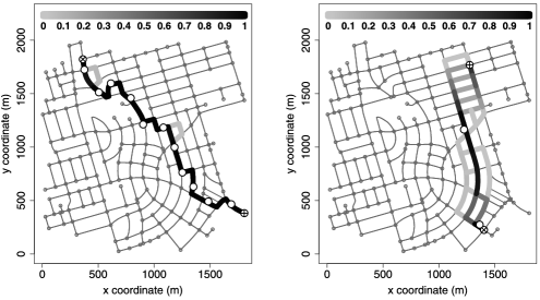
Figure 2: Map-matching estimates for two simulated trips, shaded by the probability each arc is traversed.

The Bayesian method also outperforms the other methods in interval estimates. For the good GPS data, the interval estimates from the Bayesian and local methods are similar, while the estimates from the method of Budge et al. are substantially wider, with slightly higher coverage percentage. For the bad GPS data, the intervals from the Bayesian method have higher coverage percentage than the intervals from the local methods, and the intervals from the method of Budge et al. are again wider, with no corresponding increase in coverage percentage.

6.3 Map-matched path results

Next we assess path estimates from the Bayesian method for representative paths, shown in Figure 2. The GPS locations are shown in white. The starting node is marked with a cross and the ending node with an X. Each arc is shaded in gray by the marginal posterior probability that it is traversed in the path. Arcs with probability less than 1% are unshaded. The left-hand path is from a good GPS data set, as defined in Section 6.1. The Bayesian method easily identifies the correct path. Every correct arc has close to 100% probability, and only two incorrect detours have probability above 1%. This is typical performance for trips with good GPS data. The right-hand path is from a bad GPS data set. The sparsity in GPS readings makes the path very uncertain. Near the beginning of the path, there are five routes with similar expected travel times, and the GPS readings do not distinguish between them, so each has roughly 20% posterior probability. The Bayesian method is very effective at identifying alternative routes when the true path is unclear.

7 Analysis of Toronto EMS data

Next we compare the four methods on the Toronto EMS data.

7.1 Data

The Toronto data consist of GPS data and trip information for ambulance trips with one of two priority levels: lights-and-sirens (L–S) or standard travel (Std). We address these separately, again focusing on the Leaside subregion of Toronto. The right plot in Figure 1 shows the GPS locations for the L–S data set. This data set contains 1930 ambulance trips and roughly 14,000 GPS points. The primary roads tend to have a large amount of data, the secondary roads a moderate amount, and the tertiary roads a small amount. The Std data set is larger (3989 trips), with a similar spatial distribution of points.

We use only the portion of trips where the ambulance was driving to the scene of an emergency, and discard trips for which this portion cannot be identified. We also discard some trips (roughly 1%) that would impair estimation, for example, trips where the ambulance turned around or where the ambulance stopped for a long period, not at a stoplight or in traffic. Finally, most of the trips in the data set do not begin or end in the subregion, they simply pass through, so we use the closest node to the first GPS location as the approximated start node, and the time of the first GPS reading as the start time. Similarly, we use the last GPS reading for the end node. This produces some inaccuracy of estimated travel times on the boundary of the region. This could be fixed by applying our method to overlapping regions and discarding estimates on the boundary.

7.2 Arc travel time estimates

Here we report the travel time estimates from the Bayesian method. Toronto EMS has existing estimates of the travel times, which we use to set the prior $\{m_{j}\}_{j=1}^{J}$ hyperparameters (see the supplementary material [Westgate et al. (2013)]). These estimates are different for L–S and Std trips, but are the same for the two travel directions of parallel arcs. We have also tested the Bayesian method with the data-based hyperparameters described in the supplementary material [Westgate et al. (2013)] and have observed similar performance. Figure 3 shows prior and posterior speed estimates (length divided by mean travel time) from the Bayesian method on the L–S data set. Each arc is shaded in gray based on its speed estimate, so most roads have two shades in the right-hand plot, corresponding to travel in each direction.

The posterior speed estimates from the Bayesian method are reasonable; primary arcs tend to have high speed estimates, and estimated speeds for consecutive arcs on the same road are typically similar. Arcs heading into major intersections (intersections between two primary or secondary roads, as shown in Figure 1) are often slower than the reverse arcs. In the corresponding figure for Std data (not shown), the slowdown into major intersections is even more pronounced. For most arcs the posterior estimate of the speed is higher than the prior estimate, suggesting that the existing road speed estimates used to specify the prior are underestimates.

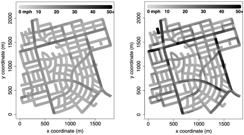
Figure 3: Prior (left) and posterior (right) speeds from the Bayesian method, for Toronto L–S data, in miles per hour (mph).

There are a few arcs that have poor estimates from the Bayesian method. For example, parallel black arcs in the top-left corner have poor estimates due to edge effects. Also, some short interior arcs have unrealistically high estimates, likely because there are few GPS points on these arcs. This undesirable behavior could be reduced or eliminated by using a random effect prior distribution [Gelman et al. (2004)] for roads in the same class, which would have the effect of pooling the available data.

7.3 Travel time prediction

We compare the known travel time of each trip in the test data with the point and 95% interval predictions from each method. Unlike the simulated test data in Section 6, the true paths are not known. For the Bayesian and local methods, we assume that the path taken is the fastest path in expectation. This measures the ability of each method to estimate both the fastest path and the travel time distributions.

We again use the cross-validation approach of Section 5 to estimate bias correction factors. We repeat this five times, resampling random training and validation/test sets, and give arithmetic means of the performance metrics over the five replications in Table 2. We again compare the point estimates from the three methods on the test data using RMSE, RMSE log, and Bias (M.A.), and compare the interval estimates using Width and Cov. %. Because the true travel time distributions are unknown, we cannot use the Oracle method as in Section 6.2. However, we still wish to estimate gold standard performance, so we implement an Estimated Oracle method, in which we assume that the parametric model and MLE estimates from the Local MLE method are the truth. We simulate realized travel times on the fastest path (in expectation, as estimated by the Local MLE method) for each test trip and compare these to the point estimates from the Local MLE method. To avoid simulation error, we use Monte Carlo estimates from 1000 simulated travel times for each trip.

Table 2: Out-of-sample trip travel time estimation performance on Toronto EMS data

Estimation method	RMSE (s)	RMSE log	Bias (M.A.)	Cov. %	Width (s)
L–S data (Mean over five replications)
Est. oracle	014.9	0.168	0.018	–	–
Bayesian	037.8	0.332	0.025	85.8	075.0
Local MLE	038.4	0.342	0.027	73.3	055.0
Local harm.	038.5	0.343	0.028	77.5	075.2
Budge et al.	039.8	0.342	0.028	94.5	122.3
Std data (Mean over five replications)
Est. oracle	035.2	0.191	0.018	–	–
Bayesian	126.8	0.465	0.025	73.0	141.8
Local MLE	129.0	0.480	0.025	58.4	118.6
Local harm.	129.0	0.480	0.025	64.8	142.8
Budge et al.	127.9	0.475	0.026	94.3	370.8

For the L–S data, the Bayesian method outperforms the method of Budge et al. and the local methods, suggesting that it is effectively combining trip information with GPS information. The Bayesian method is roughly 6% better in log scale RMSE, after subtracting the error from the Estimated Oracle method. The method of Budge et al. and the local methods perform similarly. The bias correction is successful at eliminating bias (there is 2–3% bias remaining).

The Bayesian method substantially outperforms the local methods in interval estimates. The Bayesian intervals have much higher coverage percentage than the intervals from the local methods. The method of Budge et al. has higher coverage percentage than the Bayesian method, however, the intervals are also wider. The intervals from the MLE method are narrow and have low coverage percentage. Therefore, the Local MLE method does not adequately account for travel time variability, suggesting that the Estimated Oracle method may underestimate the baseline error. If so, the Bayesian method outperforms the other methods by an even larger amount, relative to the baseline error.

For the Std data, the Bayesian method outperforms the local methods by roughly 5% in RMSE on the log scale, and outperforms the method of Budge et al. by 3.5%, again relative to the Estimated Oracle error. Point estimates from the method of Budge et al. slightly outperform the local methods. Interval estimation is less successful for the Bayesian and local methods than for the L–S data, probably because the Std travel times have more unaccounted sources of variability than the L–S travel times, such as traffic and time of day.

This region and data set are generally favorable to the method of Budge et al. The travel speeds are similar across most roads in this region, which mitigates the main weakness of the Budge et al. method, namely, its inability to distinguish between fast and slow roads. Also, several particular paths are very common in the Leaside region, and the Budge et al. method fits the travel time distribution of these particular paths very closely, leading to relatively high predictive accuracy. On the full city the routes would be much more heterogeneous, with many different routes of roughly the same travel distance, so that a method that can model the heterogeneity is expected to have a greater advantage.

7.4 Response within time threshold

Next we estimate the probability an ambulance completes its trip within a certain time threshold [Budge, Ingolfsson and Zerom (2010)]. These probabilities are critical for EMS providers (see Section 1). In Figure 4, we assume that an ambulance begins at the node marked with a black X and estimate the probability it reaches each other node in 150 seconds, following the fastest path in expectation. For the Bayesian method, these probabilities are calculated by simulating travel times from the posterior distribution of each arc in the route, and using Monte Carlo estimation (see Section 3). The left-hand figure shows probabilities from the Bayesian method, and the right-hand figure shows probabilities from the method of Budge et al.

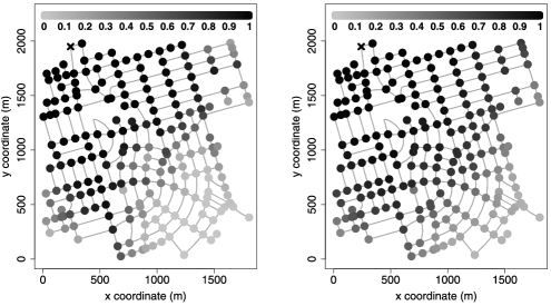
Figure 4: Estimates of probability of reaching each node in 150 seconds, Bayesian method (left), Budge et al. method (right), from the location marked X.

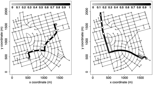
Figure 5: Map-matching estimates for two Toronto L–S trips, shaded by the probability each arc is traversed.

The probabilities for both methods appear reasonable; they are high for nodes close to the start node and decrease for nodes further away. The probabilities from the Bayesian method appear more realistic than those from Budge et al., since nodes on main roads tend to have higher probabilities from the Bayesian method (e.g., traveling south from the start node), whereas nodes on minor roads far from the start node have lower probabilities from the Bayesian method (see the bottom-right in each plot). This is because the method of Budge et al. does not take into account the different speeds of different roads.

7.5 Map-matched path accuracy

Finally, we assess map-matching estimates from the Bayesian method, for the Toronto L–S data. Figure 5 shows two example ambulance paths from the L–S data set. The GPS locations are shown in white; the first reading is marked with a cross and the last with an X. As in Section 6.3, each arc is shaded by its marginal posterior probability, if it is greater than 1%. In the left-hand path, there are two occasions where the path is not precisely defined by the GPS readings. On both occasions, roughly 90% of the posterior probability is given to a route following the main road, which is estimated to be faster. The final two GPS readings appear to have location error. However, the fastest path is still given roughly 100% posterior probability, instead of a detour that would be slightly closer to the second-to-last GPS reading. In the right-hand path, for an unknown reason, there is a large gap between GPS points. Most of the posterior probability is given to the fastest route along the main roads. This illustrates the robustness of the Bayesian method to sparse GPS data.

8 Conclusions

We proposed a Bayesian method to estimate the travel time distribution on any route in a road network using sparse and error-prone GPS data. We simultaneously estimated the vehicle paths and the parameters of the travel time distributions. We also introduced two local methods based on mapping each GPS reading to the nearest road segment. The first method used the harmonic mean of the GPS speeds; the second performed maximum-likelihood estimation for a lognormal distribution of travel speeds on each segment.

We compared these three methods to an existing method from Budge, Ingolfsson and Zerom (2010). In simulations, the Bayesian method greatly outperformed the local methods and the method of Budge et al. in estimating out-of-sample trip travel times, for both point and interval estimates. The estimates from the Bayesian method remained excellent even when the GPS data had high error. On the Toronto EMS data, the Bayesian method again outperformed the competing methods in out-of-sample prediction and provided more realistic estimates of the probability of completing a trip within a time threshold than the method of Budge et al.

We plan to extend the Bayesian method to include time-varying travel times. For instance, speeds typically decrease during rush hour. Applying the methods of this paper separately to rush hour and nonrush hour improves performance on standard travel Toronto data, although it has little effect on performance for lights-and-sirens data. A more sophisticated approach that smooths across time of day may have better success.

We are currently investigating a number of other extensions. First, we are developing methods to approximate or modify the Bayesian method to obtain efficient computation on very large networks. Second, we are experimenting with information sharing across roads to improve estimates on infrequently used roads. Third, we are incorporating dependence between arc travel times within each trip, arising from traffic congestion effects or a driver’s speed preference, for example. This change is expected to improve coverage of interval estimates. Finally, we are investigating the use of turn penalties. For example, a left turn can require more time than a right turn.

References

- Aladdini (2010) {bmisc}[author] \bauthor\bsnmAladdini, \bfnmK.\binitsK. (\byear2010). \bhowpublishedEMS response time models: A case study and analysis for the region of Waterloo. Master’s thesis, Univ. Waterloo. \bptokimsref \endbibitem
- Alanis, Ingolfsson and Kolfal (2012) {barticle}[author] \bauthor\bsnmAlanis, \bfnmR.\binitsR., \bauthor\bsnmIngolfsson, \bfnmA.\binitsA. and \bauthor\bsnmKolfal, \bfnmB.\binitsB. (\byear2012). \btitleA Markov Chain model for an EMS system with repositioning. \bjournalProduction and Operations Management \bvolume22 \bpages216–231. \bptokimsref \endbibitem
- Breslow and Lin (1995) {barticle}[mr] \bauthor\bsnmBreslow, \bfnmNorman E.\binitsN. E. and \bauthor\bsnmLin, \bfnmXihong\binitsX. (\byear1995). \btitleBias correction in generalised linear mixed models with a single component of dispersion. \bjournalBiometrika \bvolume82 \bpages81–91. \biddoi=10.1093/biomet/82.1.81, issn=0006-3444, mr=1332840 \bptokimsref \endbibitem
- Brotcorne, Laporte and Semet (2003) {barticle}[mr] \bauthor\bsnmBrotcorne, \bfnmLuce\binitsL., \bauthor\bsnmLaporte, \bfnmGilbert\binitsG. and \bauthor\bsnmSemet, \bfnmFrédéric\binitsF. (\byear2003). \btitleAmbulance location and relocation models. \bjournalEuropean J. Oper. Res. \bvolume147 \bpages451–463. \biddoi=10.1016/S0377-2217(02)00364-8, issn=0377-2217, mr=1965248 \bptokimsref \endbibitem