Hierarchical Bayesian analysis of somatic mutation data in cancer

Abstract

Identifying genes underlying cancer development is critical to cancer biology and has important implications across prevention, diagnosis and treatment. Cancer sequencing studies aim at discovering genes with high frequencies of somatic mutations in specific types of cancer, as these genes are potential driving factors (drivers) for cancer development. We introduce a hierarchical Bayesian methodology to estimate gene-specific mutation rates and driver probabilities from somatic mutation data and to shed light on the overall proportion of drivers among sequenced genes. Our methodology applies to different experimental designs used in practice, including one-stage, two-stage and candidate gene designs. Also, sample sizes are typically small relative to the rarity of individual mutations. Via a shrinkage method borrowing strength from the whole genome in assessing individual genes, we reinforce inference and address the selection effects induced by multistage designs. Our simulation studies show that the posterior driver probabilities provide a nearly unbiased false discovery rate estimate. We apply our methods to pancreatic and breast cancer data, contrast our results to previous estimates and provide estimated proportions of drivers for these two types of cancer.

T1Supported by the National Science Foundation [award 0342111].

, ,
and

1 Introduction

We introduce a semiparametric hierarchical Bayesian model for the analysis of somatic mutations in cancer. Our study is motivated by experiments sequencing comprehensive libraries of coding genes in tumors and matching normal samples [Cancer Genome Atlas Research Network (2008, 2011), Sjöblom et al. (2006), Greenman et al. (2007), Wood et al. (2007), Jones et al. (2008), Parsons et al. (2008), Kan et al. (2010)]. A main goal of these studies has been to provide lists of candidate cancer genes, for which evidence of a role in driving carcinogenesis emerged from the the presence of somatically acquired differences between tumor and normal genomes. These driver genes need to be distinguished from so-called passenger genes, which present somatic mutations in cancer even though these mutations are not directly related with the tumor genesis. Statistical tools for this task have been based on hypotheses testing theory and, in particular, on methods for controlling the false discovery rates (FDR) of reported gene lists [Greenman et al. (2006), Wood et al. (2007), Getz et al. (2007), Parmigiani et al. (2009), Trippa and Parmigiani (2011)]. Our goal here is to complement this approach with methodology for deriving the probability that a gene contributes to carcinogenesis. There are four important reasons for this: to handle multistage designs; to remedy the severe FDR overestimation resulting from one-gene-at-a-time analyses; to improve ranking and selection of genes for subsequent analyses; and to address estimation of the total number of cancer drivers.

First, the rarity of mutations and the cost of sequencing comprehensive lists of genes have motivated the use of multistage designs, to balance between resource use and power in detecting cancer genes [Kraft (2006), Skol et al. (2006), Wang and Stram (2006), Sjöblom et al. (2006), Parmigiani et al. (2009)]. In these studies, genes are selected for later stages based on results of earlier stages as well as a host of other biological considerations, including membership in key pathways, potential for drug targeting, reliability of sequencing and findings of previous sequencing studies. Kan et al. (2010), for instance, discussed the analysis of 1507 genes selected in part on the basis of previously published results. Methods based on $p$-values do not include prediction of the final findings at completion of the first stage. This limit, in multi-stage problems, compounds with conceptual challenges when biological judgment is used to refine lists of candidates that are moved along to the last stages of the study. Also, multiple hypothesis testing methods are not designed for optimally selecting genes for subsequent stages, while Bayesian analysis allows one to obtain the probabilities (i) that a gene is a driver and (ii) that it will be validated in subsequent stages. Posterior driver probabilities provide two unique advantages. Prior to a new study or stage with a pre-specified hypothetical sample size, they allow, unlike $p$-values, to assess the probability, for each gene, of finding a number of mutations that would provide evidence of an abnormal mutation rate. After a study, they are applicable for summarizing the study findings, irrespective of the selection criteria used to move genes through stages.

Second, the standard inferential approach for mutation analysis is to compute false discovery rates based on standard multiple testing correction, following one-gene-at-a-time analyses such as likelihood ratio tests. This approach can lead to a severe overestimation of the FDR.

Third, an important goal of somatic mutation analysis is to determine genes’ mutation rates. In a typical genome-wide study, sample sizes are small relative to the rarity of individual mutations. For example, we expect to observe no mutations for most of the genes, though estimating a population-level mutation rate of zero would be biologically implausible. Also, in multi-stage designs, it is important to account for possible biases arising from selecting genes with high mutation frequencies in early stages. Both issues can be addressed using a model-based approach for estimating individual genes’ mutation rates by “borrowing strength” from the entire set of mutations across the genome [Efron and Morris (1973)]. Shrinkage affects posterior driver probabilities and mutation rates estimates, as genes for which less information is available are pulled more strongly toward the genome-wide average.

Fourth, the change of landscape resulting from early cancer genome projects has posed the question of the proportion of driver genes across the genome. Wood et al. (2007) had pointed at this question and proposed conservative estimators applied for FDR control with empirical Bayes testing procedures. Our methodology is designed to also provide an estimate of this proportion with the associated statement of uncertainty.

The organization of the remaining sections is as follows. Section 2 gives a general description of cancer somatic mutation data. Section 3 describes our Bayesian hierarchical model. Section 4 shows the results of simulated experiments designed to assess the improvement provided by our approach over standard alternatives. Section 5 presents a re-analysis of two published sequencing studies. Finally, Section 6 provides additional discussion about our method and results.

2 Cancer somatic mutation data

We consider studies providing a collection of somatic mutations from genome-wide exome sequencing of samples of a specific tumor type. Somatic mutations can be detected by comparing DNA sequences of tumor samples to those of their matching normal samples. Each mutation is labeled as one of a set of possible mutation types, as in the example of Table 1. Mutations of different types are observed to

=139pt Mutated from Mutated to C in CpG A – G T G in CpG A C – T G in GpA A C – T C in TpC A – G T A – C G T Other C A – G T Other G A C – T T A C G –

Table 1: 24 point mutation types

have varying overall frequencies in tumor samples. Different definitions of mutation types may be used to suit different data structures or different biological questions. In this paper, as in Wood et al. (2007) and Jones et al. (2008), each mutation is classified either as a small insertion/deletion or as one of 24 types of single nucleotide changes, defined in Table 1. For each gene, mutation type and sample, it is important to consider the mutation count as well as the number of nucleotides at risk for that type of mutation, heretofore called the coverage. The coverage for a gene may be smaller than the total base count because not all bases may be reliably sequenced.

We analyze data generated in two previous studies. The first [Jones et al. (2008)] includes 24 tumors with matching normal tissues from patients with pancreatic malignancies. The study sequenced 20,671 genes and found 1163 nonsynonymous somatic mutations harbored in 1007 genes. These mutations were categorized by gene, mutation type and sample. The second study [Wood et al. (2007)] considered breast cancer, and adopted a two-stage design with 11 samples in the discovery stage and 24 samples in the subsequent validation stage. During the discovery stage, 18,190 genes were sequenced and 1112 nonsynonymous mutations were identified in 1026 genes. During the validation stage, these 1026 genes were sequenced in the additional 24 tumors, and 190 nonsynonymous mutations were identified in 154 genes. Mutations were categorized by gene, mutation types and stage. The data, at the gene level, include two mutation counts, one for each stage. An advantage of performing Bayesian analyses of these data sets is that both the probability model and the computational procedures can be straightforwardly adapted to these designs, as well as other multi-stage designs.

3 Model

Somatic mutation counts are modeled using a Bayesian multilevel semi-parametric model. At the data level, the observed count of somatic mutations of type $m$ in gene $g$ and sample $k$, indicated by $X_{\mathit{gmk}}$, has distribution

$$X_{\mathit{gmk}} \sim \operatorname{Poisson}(\lambda_{\mathit{gmk}}T_{\mathit{gmk}}),$$ (2)

$$\eqntext{g=1,\ldots,G;m=1,\ldots,M;k=1,\ldots,K,}$$

where $\lambda_{\mathit{gmk}}$ is the unknown mutation rate and $T_{\mathit{gmk}}$ is the observed coverage for the corresponding gene, mutation type and sample, that is, the number of successfully sequenced bases in gene $g$ and sample $k$, that are susceptible to a mutation of type $m$. The term “coverage,” in the next-generation sequencing literature, has a different interpretation. Here we use it consistently with earlier studies using Sanger sequencing technology [e.g., Wood et al. (2007)].

The binomial and multinomial distributions are often used for mutation counts in somatic mutation analysis [Greenman et al. (2006)]. Here we use a Poisson distribution because it is a good approximation of both those distributions when the mutation rates are small and because it simplifies the calculation of the posterior distributions. Our model assumes that mutations within a single gene and among different genes occur independently of each other conditional on mutation rates.

At the mutation rate level, we use a multiplicative random effects model

$$\lambda_{\mathit{gmk}}=\lambda_{g}\alpha_{m}\beta_{k},$$ (3)

which includes a gene specific mutation rate $\lambda_{g}$, a mutation type effect $\alpha_{m}$ and a sample effect $\beta_{k}$. The three multiplicative components have the following interpretation: the $\lambda_{g}$’s allow to assign each gene its own mutation rate; the $\alpha_{m}$’s allow the rates to vary across mutation types; the $\beta_{k}$’s allow different samples to have different mutation rates, a feature observed in most data sets. We set $\prod_{m=1}^{M}\alpha_{m}=1$ and $\prod_{k=1}^{K}\beta_{k}=1$ to make the model identifiable.

We propose and compare two complementary approaches, one for estimating gene-specific mutation rates and one for estimating gene-specific driver probabilities. One of the main differences is that the first approach does not require a reliable estimate of the passenger mutation rate while the second does. The assumption of known passenger rates has also been used in the previous literature [e.g., Jones et al. (2008), Cancer Genome Atlas Research Network (2008)] for identifying driver genes with FDR methods.

To complete the multilevel model, we specify a distribution for mutation rates across genes. We treat this distribution as unknown and estimate it from the data with minimal distributional assumptions. Early cancer genome studies, for example, Wood et al. (2007), have shown the existence of small subgroups of driver genes, the so-called “mountains,” with rates of mutations over 100-fold higher than the assumed passenger rates. In contrast, most of the likely drivers are found to harbor mutations only in small proportions of samples and hence are called “hills.” This motivates the use of nonparametric modeling to mitigate the overall influence of mountains on the inference. We use a Dirichlet Process [Ferguson (1973)] for the unknown distribution of the mutation rates across the genome:

$$F \sim \mbox{Dirichlet Process}\bigl{(}a,\operatorname{Exponential}(\gamma)\bigr{)},$$

$$\lambda_{g}|F \stackrel{{\scriptstyle\mathrm{i.i.d.}}}{{\sim}} F,$$

where $a$ is the so-called concentration parameter and $\gamma$ controls the mean of the random distribution $F$, chosen to be exponential. The nonparametric Dirichlet prior is flexible and has proven useful in several applications modeling random effects distribution, as done here. See Dunson (2010) for an extensive overview.

We can now consider the second case, in which the main interest is to derive driver probabilities at the gene level. Here we make the additional assumption that for all passenger genes, $\lambda_{g}=\lambda_{0}$, a known mutation rate. If this assumption holds, the driver genes can be defined statistically as those with mutation rates greater than $\lambda_{0}$, because any gene whose mutations have the ability to provide a fitness advantage to cancer cells will occur in cancer at adjusted rates higher than $\lambda_{0}$ when a large enough population is considered. The word adjusted here refers to the fact that, because of different coverage and nucleotide composition, different passengers may still exhibit different mutation rates per nucleotide even though the baseline mutation rate $\lambda_{0}$ is common to all.

To derive driver probabilities, we slightly modify the model above and include an additional hierarchical level. We use binary variables $\delta_{g}$, one for each gene, for distinguishing the drivers ($\delta_{g}=1$) from the passengers ($\delta_{g}=0$). The $\lambda_{g}$ is now

$$\lambda_{g}=\mathrm{I}(\delta_{g}=0)\lambda_{0}+\mathrm{I}(\delta_{g}=1)\bigl{(}\lambda_{g}^{d}+\lambda_{0}\bigr{)},$$ (5)

where $\lambda_{g}^{d}$ is the difference between the mutation rate of a putative driver $\lambda_{g}$ and the pre-specified underlying passengers rate $\lambda_{0}$. Since $\delta_{g}$ is also unknown, a natural choice for modeling the binary variables is the conjugate Beta-Bernoulli prior

$$\pi \sim \operatorname{Beta}(a_{\pi},b_{\pi}),$$

$$\delta_{g}|\pi \stackrel{{\scriptstyle\mathrm{i.i.d.}}}{{\sim}} \operatorname{Bernoulli}(\pi),$$

where $\pi$ is the unknown overall proportion of drivers among all genes. We use a Dirichelet prior for the latent $\lambda_{g}^{d}$’s:

$$F \sim \mbox{Dirichlet Process}\bigl{(}a,\operatorname{Exponential}(\gamma)\bigr{)},$$

$$\lambda_{g}^{d}|F \stackrel{{\scriptstyle\mathrm{i.i.d.}}}{{\sim}} F.$$

Diffuse flat prior densities are used for random vectors $(\alpha_{1},\ldots,\alpha_{M})$ and $(\beta_{1},\ldots,\beta_{K})$. We also use a Gamma hyper-prior for $\gamma$. The value of $a$ in the Dirichlet process is set to 1. In simulations, we considered several values of $a$ and performed sensitivity analyses. We observed negligible variations in our results across prior parameterizations.

The posterior distributions of parameters from the hierarchical Bayesian models are estimated using a Markov Chain Monte Carlo algorithm. See the supplementary material [Ding et al. (2013)] for details.

4 Simulation study

4.1 Scenarios

We used simulations for validating our Bayesian procedure. Simulation scenarios have strong similarities with the pancreatic study in Jones et al. (2008). We used the same set of genes and their corresponding coverage. We set the passenger mutation rate to $\lambda_{0}=3.68\times 10^{-7}$, a realistic rate corresponding to the geometric mean of the estimated passenger rates across mutation types used in Jones et al. (2008). A geometric mean was used because of the constraint on mutation type effects, that is, $\prod\alpha_{m}=1$. Next, $\alpha_{m}$’s were estimated from the data and samples effects $\beta_{k}$’s were proportional to the numbers of mutations in the 24 samples in the pancreatic cancer data. Their products were set to 1 to satisfy the constraints. In summary, the sampling model for the passenger genes in our simulation scenario is tailored to the data and assumptions used in Jones et al. (2008). The mutation rates of a small set of randomly selected genes were inflated to represent true drivers: 2% of genes were set to have mutation rate $10\lambda_{0}$, 1% of genes were set to have mutation rate of $30\lambda_{0}$ and 0.05% of genes were set to have mutation rate $200\lambda_{0}$. A 200-fold increase is realistic for the so-called “mountain” genes, while 10-fold and 30-fold increases correspond to the “hills.” The proportions of true drivers at different mutation rates were chosen manually to make the overall distribution of observed mutation counts close to that observed in the pancreatic cancer data.

Figure 1: (a) Logarithm of estimated mutation rate ($\lambda_{\mathrm{HB}}$) against the observed number of mutations. (b) Cumulative distribution of the logarithm of $\lambda_{\mathrm{HB}}$ with genes grouped by their true $\lambda_{g}$’s. In (a), each point is one gene, and the Y axis levels are slightly shifted to separate the groups. Vertical dashed lines indicate true $\lambda_{g}$’s used in the simulation. The legend in (a) applies to both (a) and (b).

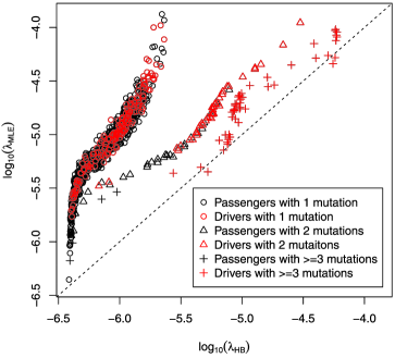
Figure 2: Hierarchical Bayesian estimates versus maximum likelihood estimates of mutation rates. Each point is a gene, labeled according to its number of mutations and colored according to whether it is a true driver. Drivers are over-plotted or else drivers with a single mutation would be invisible, given the large number of other genes.

4.2 Results

Figure 1 shows results of mutation rate estimates from the simulated data. Estimated $\lambda_{g}$’s of individual genes are shown in Figure 1(a) against their observed mutation counts. The average estimated mutation rate for genes with no mutation is $3.83\times 10^{-7}$, very close to the true $\lambda_{0}=3.68\times 10^{-7}$ used in the simulation, even though $\lambda_{0}$ was not known to the estimation procedure. This suggests that the model captures the underlying passenger mutation rate. Also, for genes with no mutation, there is no separation among genes with different true mutation rates, which is expected since there is no information to distinguish them. Estimated mutation rates generally increase as the number of mutations increases, but there are also large differences in estimated rates among genes with the same number of mutations, resulting from different sizes and nucleotide compositions of those genes.

Figure 1(b) shows the estimated $\lambda_{g}$’s by groups defined by the true $\lambda_{g}$’s. Each line is the cumulative distribution of the logarithms of the estimated $\lambda_{g}$’s for one of the groups. Even among genes with 200-fold increases over the passenger rate, two genes are not distinguishable from passengers because they did not have any mutations in the 24 simulated samples. This illustrates the challenges of learning gene-specific mutation rates in this type of study.

As an alternative approach to estimating mutation rates we considered the maximum likelihood estimates (MLE) calculated for each gene separately. We assumed the same Poisson model for the MLE. For the calculation of the MLEs, the true parameters $\alpha_{m}$’s and $\beta_{k}$’s were plugged in, a choice that favors the MLEs. Figure 2 compares posterior means of $\lambda_{g}$’s obtained using our Hierarchical Bayesian model to the MLEs. Only genes with at least one observed mutation are shown. The differences between the two approaches are striking. Ranking genes by estimated rates, and proceeding down the list based on the Bayesian estimates, one does not encounter a true passenger until position 39. On the other hand, the top two genes by MLE are both true passengers and among the top 30 genes; only 22 are true drivers. The behavior of the two approaches is most different for genes with a single mutation, as expected. The hierarchical model has pulled these strongly toward the overall genome mean, so that the genes with one mutation rank below most of the genes with more than one mutation. For genes with two mutations, the shrinkage is less pronounced, and for genes with 3 or more mutations, the estimates are generally close, with the exception of a small number of large genes who are pulled strongly, and in a nonlinear pattern, toward smaller values.

The main difference between our hierarchical Bayesian approach and the MLE is shrinkage. By using a mixing distribution representative of the distribution of the genes’ rates across the genome, the Bayesian approach estimates each mutation rate using data from many other genes with potentially similar rates. This underlying distribution is not considered by the MLE approach.

Figure 3: (a) Estimated driver probability against the observed number of mutations. (b) Cumulative distribution of the estimated driver probabilities with genes grouped by their true $\lambda_{g}$’s. In (a), each point is one gene, and the Y axis levels are slightly shifted to separate the groups. The legend in (a) applies to both (a) and (b).

Figure 3 shows the posterior driver probabilities from the same simulated data set. The true passenger mutation rate used in the simulation was used as $\lambda_{0}$ in the Bayesian model. Overall the results have similar patterns compared to those of the estimated mutation rates. Figure 3(a) shows estimated driver probabilities of all genes against their observed mutation counts. Genes with no mutation have estimated driver probabilities close to 0 regardless of their true mutation rates. As the number of mutations increases, the estimated driver probabilities generally also increase. Only a small number of genes have estimated probabilities close to 1. Figure 3(b) groups genes by their true mutation rates to present the differences among the four groups. For genes with true mutation rates equal to $200\lambda_{0}$, estimated driver probabilities are large, except for the two genes with no observed mutation. A substantial proportion of the genes with mutation rates equal to $10\lambda_{0}$ and $30\lambda_{0}$ have estimated driver probabilities much larger than 0.

The estimated proportion of driver genes, $\pi$, is 0.025 with a 90% credible interval $(0.017,0.041)$, while the true value used in the simulation is 0.0305. We also used several different Beta distributions as priors for $\pi$ and they all led to similar posterior estimates. Using different values as $\lambda_{0}$ in the model resulted in very different estimates of $\pi$. Doubling $\lambda_{0}$ led to an estimated $\pi$ of 0.0065 with a 90% credible interval $(0.0047,0.0087)$, while reducing $\lambda_{0}$ by half led to an estimated $\pi$ of 0.48 with a 90% credible interval $(0.37,0.59)$. These results show the dependence of the estimated $\pi$ on the input parameter $\lambda_{0}$.

We also used likelihood ratio tests (LRT) with Poisson densities to analyze the simulated data. We used the true $\alpha_{m}$’s and $\beta_{k}$’s for LRTs here. For gene $g$, under the null hypothesis, $\lambda_{g}=\lambda_{0}$, the total number of mutations $X_{g}=\sum_{m,k}(X_{\mathit{gmk}})$ follows a Poisson distribution with parameter $\sum_{m,k}\alpha_{m}\beta_{k}T_{\mathit{gmk}}$. The $p$-value for the likelihood ratio test can be calculated using the right-tail probability of $X_{g}$ under the null hypothesis. We then used the FDR controlling procedure from Benjamini and Hochberg (1995) to calculate estimated FDRs from LRT $p$-values. To compare the results to those from our method, we also calculated estimated FDR from Hierarchical Bayesian estimates of the driver probabilities. True FDRs were calculated using the true driver indicators used in the simulation. Figure 4 shows the results from these two methods. The estimated FDRs from our hierarchical Bayesian method are very close to the true FDRs, showed by the closeness of the curve to the diagonal line. The estimated rates from likelihood ratio tests are much smaller than the true rates, suggesting that they are too conservative by as much as an order of magnitude.

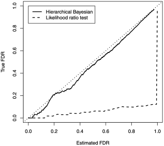
Figure 4: True FDRs and estimated FDRs from hierarchical Bayesian estimates of driver probabilities and likelihood ratio test $p$-values for all genes.

The main reason for the overestimation of FDR here is that the controlling procedure assumes a uniform distribution of $p$-values from true null tests. However, because the distribution of mutation counts for each gene is Poisson and the mutation rate is very small under the null hypothesis, the vast majority of true passenger genes have mutation counts of 0. The resulting distribution of $p$-values from true passenger genes is very different from a uniform distribution. This shows that our method has substantially better calibration and improved ability to estimate driver probabilities and the overall proportion of driver genes compared to LRT coupled with an FDR controlling procedure. This improvement is critical for the appropriate interpretation of lists of candidate drivers and for the efficient design of two-stage studies.

5 Cancer mutation data analysis

5.1 Pancreatic cancer data

Figure 5 shows the estimates of mutation rates with the pancreatic cancer data. Genes are ordered by their estimated mutation rates and the 50 genes with the largest estimated rates are listed on the top. The mean of estimated mutation rates for genes with no mutations is $3.93\times 10^{-7}$, closer to the “intermediate” passenger mutation rate $\lambda_{0}=3.68\times 10^{-7}$ than the “low” rate $2.07\times 10^{-7}$ and the “high” rate $5.30\times 10^{-7}$ provided in Jones et al. (2008). Among the top 50 genes, only a few have 90% credible intervals completely above the “intermediate” rate. Genes with small sizes, such as CDKN2A, tend to have large credible intervals.

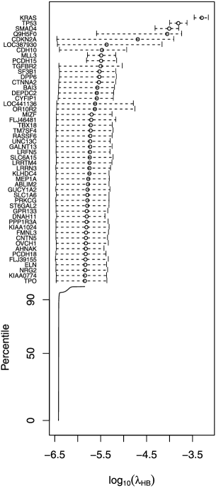
Figure 5: Estimated mutation rates from the pancreatic cancer data. Genes are ordered according to their estimated mutation rates ($\lambda_{\mathrm{HB}}$). The names and 90% credible intervals of the top 50 genes are shown.

We also calculated maximum likelihood estimates of the mutation rates $\lambda_{g}$ for each gene with at least one observed mutation. See supplementary material [Ding et al. (2013)] for the details of MLE calculation. The comparison between MLEs and hierarchical Bayesian estimates is shown in Figure 6. The overall shape reproduces the pattern seen in the simulation study. The shrinkage effect is evident for most genes with only 1 mutation, and it is greater for small genes. For example, the gene OSTN, with only 300 bases sequenced, has a MLE of $5.7\times 10^{-5}$, the 11th highest rate, while the Bayesian estimate is only $7.3\times 10^{-7}$, much closer to the whole-genome average rate, and is ranked 117th. On the other end, the gene PCDHGC4, with more than 52,000 bases sequenced, had a MLE of $2.2\times 10^{-7}$ and a Bayesian estimate of $3.8\times 10^{-7}$, also closer to the genome average. The MLEs and Bayesian estimates for genes with 3 or more mutations are similar.

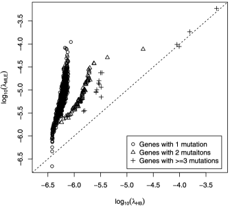
Figure 6: Hierarchical Bayesian estimates versus maximum likelihood estimates of mutation rates. Each point is a gene, labeled according to its number of mutations.

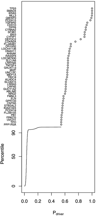
Figure 7: Estimated driver probabilities from the pancreatic cancer data. Genes are ordered according to their estimated driver probabilities ($P_{\mathrm{driver}}$). The names of the top 50 genes are shown.

Figure 7 shows the estimated driver probabilities using the “intermediate” rate from Jones et al. (2008) as the passenger rate $\lambda_{0}$ in our model. Genes are ordered by their estimated driver probabilities and the 50 genes with the highest driver probabilities are listed on the top. The list of the top 50 genes is very similar, though not identical, to that generated by the estimated mutation rates. It is interesting to contrast the inferences on genes CDKN2A and MLL3 with very different gene sizes. CDKN2A is a small gene with 206 bases sequenced, so 2 mutations are enough to produce a large estimated mutation rate. CDKN2A is ranked higher than MLL3, which is a much larger gene with 13,908 bases sequenced and 6 observed mutations. However, CDKN2As credible interval is also much larger due to its small size. As a result, the driver probability of MLL3 is close to one, while that of CDKN2A is around 0.7, placing it far lower in the ranking.

The estimated proportion of driver genes, $\pi$, is 0.038 with 90% credible interval $(0.018,0.066)$, corresponding to a total number of drivers of 779 with credible interval $(381,1359)$. The large credible interval and the numerous genes with driver probability around 50% highlight the challenge of classifying individual genes using only 24 samples. However, the study provides strong evidence that the total number of drivers in pancreatic cancer is large.

Changing input passenger mutation rate has a large effect on the estimates of driver probabilities and on the overall proportion of drivers. Using the “high” passenger mutation rate resulted in an estimated $\pi=0.0041$ with 90% credible interval $(0.0016,0.0080)$, while using the “low” rate resulted in an estimated $\pi=0.28$ with 90% credible interval $(0.21,0.37)$. These rates are likely to be conservative upper and lower bounds. While the posterior driver probabilities are affected by the choice of passenger mutation rate $\lambda_{0}$, their relative orders are much more robust. For example, using the “high” rate produced a list of top 50 genes which share 38 genes with the top 50 list using the “low” rate. Also, even when using a conservative upper bound on the passenger mutation rate, the expected number of drivers is close to 100.

The original paper analyzing the pancreas cancer data [Jones et al. (2008)] used an empirical Bayes local FDR method of Efron and Tibshirani (2002), constructed using the likelihood ratio test proposed in Getz et al. (2007). Figure 8 compares driver probabilities estimated using the hierarchical Bayesian model in this paper to the probabilities estimated in Jones et al. (2008). Only genes with 2 or more mutations are plotted in the figure. This is done so the list of genes is roughly the same as the list of genes in the table S7 in Jones et al. (2008). Note that the table in Jones et al. (2008) also used amplification and deletion data, which are not used in the comparison here. The estimates from these two methods are positively correlated. For most genes shown in the figure, estimated probabilities using our method are lower than those estimated using the empirical Bayes approach. The granularity of the estimates from Jones et al. (2008) arises from the conservative steps taken to overcome statistical and numerical difficulties of estimating a null distribution when event rates are low, and from monotonization of the FDR estimates. Our Bayesian approach, through shrinkage, smoothness and other features, provides a higher resolution. It also provides a different ranking. To illustrate, the genes TTN and MUC16 are highlighted in Figure 8 on the left. TTN has 6 mutations but also has more than 100K bases sequenced, the most in this data set. This causes a greater discounting in the hierarchical Bayes approach than the MLE-based empirical Bayes approach. This is consistent with the shrinkage pattern observed in Figure 3. The other example is MUC16, which has 2 mutations and 40K bases sequenced, the third most in this data set. Another factor that may account for some of the differences in ranking is the consideration of sample effects, not used in Jones et al. (2008).

As another summarization of the hierarchical Bayesian results, Figure 9 shows the posterior distribution of the estimated number of mutated drivers in each tumor sample. All samples except one have at least two mutated drivers among all posterior simulations. The remaining one has less than 1% posterior probability of having only one mutated driver. Most samples harbor five or more mutated drivers with high probabilities; the average number is 12.

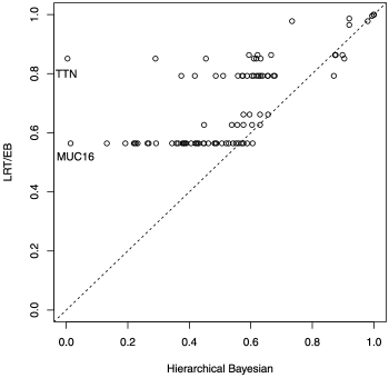
Figure 8: Comparison between estimated driver probabilities from the hierarchical Bayesian method (HB) and from the likelihood ratio test/empirical Bayes method (LRT/EB) in Jones et al. (2008).

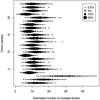
Figure 9: Posterior distribution of the estimated number of mutated drivers in each tumor sample.

5.2 Breast cancer data

The breast cancer genome project [Wood et al. (2007)] is presented here to emphasize the flexibility of the Bayesian approach in dealing with two-stage designs. The sample size was smaller than that of the pancreatic cancer data. Because of that, the results have more variability. The estimated mutation rates $\lambda_{g}$ range from $8.6\times 10^{-7}$ to $1.35\times 10^{-4}$. The average mutation rate for genes with no mutation is $1.23\times 10^{-6}$, much higher than the corresponding rate in the pancreatic cancer data. This rate is again closest to the intermediate, or “SNP-based,” passenger mutation rate among the three estimation methods in Wood et al. (2007). The estimated overall driver proportion $\pi$ varies for different passenger mutation rates used in the model. Using “External,” “SNP-based” and “NS/S-based” passenger rate estimates resulted in $\pi$ estimates of 53%, 12% and 0.02%, respectively.

6 Discussion

We developed a hierarchical Bayesian methodology to estimate gene-specific mutation rates and driver probabilities as well as the proportion of drivers among sequenced genes from somatic mutation data in cancer.

To distinguish driver genes from passenger genes solely based on marginal mutation rates, somewhat strong assumptions are needed. The first is that all passenger genes have the same mutation rate. Biologically, mutation rates can vary across different regions of genome [Wolfe, Sharp and Li (1989)] from factors such as DNA replication timing [Wolfe, Sharp and Li (1989), Stamatoyannopoulos et al. (2009)] and chromatin structure [Prendergast et al. (2007), Schuster-Böckler and Lehner (2012)]. With the sample sizes available in the data sets analyzed in this paper, it is difficult to consider variation in passenger rates explicitly, though ongoing sequencing effort may allow a deeper exploration of this issue in the near future.

Another key assumption is that mutations in different genes occur independently. Because of this assumption, we can estimate a gene’s driver probability using its marginal mutation rate. In practice, it is likely that mutations in one gene can lead to growth advantage or disadvantage depending on whether certain mutations in some other genes exist or not, especially if these genes are in the same biological pathway. While modeling of such interactions is possible for selected pathways [Boca et al. (2010), Ciriello et al. (2012)], estimation of even pairwise dependencies at the gene level across the entire genome remains challenging.

These assumptions represent a reasonable compromise between the limitations of available sequencing data and the need to prioritize candidate driver genes for further research in a model-based way. They were commonly made in other cancer somatic mutation studies [e.g., Jones et al. (2008), Cancer Genome Atlas Research Network (2008)]. With the development of new sequencing technologies and the increasing amount of cancer sequencing data, new methodologies will be needed, likely with a more flexible set of assumptions.

Our model also assumes that each sample is homogeneous such that if a mutation occurs in a gene in one sample, it occurs in all cells from that sample. This assumption realistically models the data generated by Sanger sequencing with strict quality control, where only mutations shared by the majority of cells are identified. In reality, cancer samples are often heterogeneous: the same sample can distinct subpopulation of cancer cells at different stages of evolution or even following from different evolutionary paths. So a certain mutation may only present in a proportion of cells. Such information can be obtained using deep sequencing technologies available now [Walter et al. (2012)]. To analyze such data, an additional layer could be incorporated into the hierarchical Bayesian models to account for the heterogeneity of cells in a sample. A challenge in modeling this information will arise from the fact that mutations in different genes can have different levels of heterogeneity.

We designed two models, one for estimating gene-specific mutation rates and one for estimating gene-specific driver probabilities and the overall proportion of drivers. Both achieved similar results in terms of separating groups of genes with different true mutation rates in the simulation study and ordering the top candidate driver genes in the pancreatic and breast cancer genomes data. While estimating driver probabilities provides a more direct way to answer the question of distinguishing drivers from passengers, the model does depend on the assumption that there is a single underlying passenger mutation rate common to all passenger genes and requires this rate as an input parameter.

So far, most analyses of somatic mutations rely on external estimates of the mutation rates for passenger genes, obtained, for example, from sequencing data from noncoding regions or rates of silent mutations [Wood et al. (2007)]. This input has a large effect on the estimated proportion of driver genes and the overall magnitude of the driver probabilities. However, the order of top candidates is not affected substantially either in simulated or real data. We thus recommend the use of estimated mutation rates for ranking, selection and prediction, as the model for this estimation does not require any assumption on the passenger mutation rate, nor does it need an estimate of this rate. In either model, Bayesian modeling allows us to use these external estimates, when available, for specifying the prior distribution.

Both models in this paper use a Dirichlet process on the unknown distribution of the gene-specific mutation rates across the genome. This assumption can be substituted with other types of distributions, including parametric ones. For example, we considered a log-normal distribution for mutation rate estimation and a mixture prior with point mass at $\lambda_{0}$ and a log-normal distribution truncated at $\lambda_{0}$ for driver probability estimation. When we applied these two choices to the simulated data, model fit was not as satisfactory as that of the Dirichlet process (see supplementary material [Ding et al. (2013)] for details), likely because there were a few genes with very high mutation rates (the mountains) together with a much larger set of genes with moderately increased mutation rates (the hills). The Log-normal distribution does not fit this situation well, nor would most of the commonly used parametric distributions, especially if unimodal and controlled by a small number of parameters. Thus, we strongly recommend the use of a flexible distribution, which can be estimated reliably even in relatively small studies, if the number of genes is large.

Results provided here are but examples of many summarizations one can produce using the MCMC output. For example, for each gene one can easily compute the predictive probability of observing a mutation in a hypothetical new tumor sample or new study. Another useful approach is to examine gene sets or pathways. The model output can be used to compute the probability that a chosen pathway is altered by one or more driver mutations in each of the patients, as suggested in Boca et al. (2010).

In an important paper Greenman et al. (2006) provided likelihood-based testing approaches for distinguishing drivers from passenger mutations. An interesting aspect of their work is the modeling of both the mutation process and the selection pressure on the tumor. They also considered the significance of selection toward missense, nonsense and splice site mutations, and proposed tests assessing variation in selection between functional domains. A combination of the approach considered here with the features introduced by Greenman et al. (2006), while well beyond the scope of this article, could potentially be very useful.

Our methodology provides estimates of the total number of driver genes. The early cancer genome project highlighted the importance of “hills,” or genes that are drivers in a relatively small proportion of tumors. Increasing independent evidence is accumulating to support the importance of the hills. Hills are numerous and easy to miss in small studies, which suggests that many more undiscovered hills may exist. Our model attempts a quantification of the size of this population based on mutation rates alone. This quantification is difficult, whence the large credible intervals, and sensitive to assumptions on passenger rates. Nonetheless, our method leads to the prediction that the population is large, very likely in the hundreds, and possibly in the thousands.

In conclusion, our models produce posterior inferences on all relevant parameters, using data generated from single, multi-stage and multiple studies, potentially sequencing different sets of genes. We expect that these tools will be helpful in both assessing the evidence provided by existing data and in planning further experiments to confirm the genes’ role in cancer development.

7 Software

An R package is freely available at http://bcb.dfci.harvard. edu/%7Egp/software/CancerMutationMCMC/.

[id=suppA] Supplementary methods and results [doi]10.1214/12-AOAS604SUPP .pdf aoas604_supp.pdf Additional technical details and simulation results.

References

- Benjamini and Hochberg (1995) {barticle}[mr] \bauthor\bsnmBenjamini, \bfnmYoav\binitsY. and \bauthor\bsnmHochberg, \bfnmYosef\binitsY. (\byear1995). \btitleControlling the false discovery rate: A practical and powerful approach to multiple testing. \bjournalJ. R. Stat. Soc. Ser. B Stat. Methodol. \bvolume57 \bpages289–300. \bidissn=0035-9246, mr=1325392 \bptokimsref \endbibitem
- Boca et al. (2010) {barticle}[pbm] \bauthor\bsnmBoca, \bfnmSimina M.\binitsS. M., \bauthor\bsnmKinzler, \bfnmKenneth W.\binitsK. W., \bauthor\bsnmVelculescu, \bfnmVictor E.\binitsV. E., \bauthor\bsnmVogelstein, \bfnmBert\binitsB. and \bauthor\bsnmParmigiani, \bfnmGiovanni\binitsG. (\byear2010). \btitlePatient-oriented gene set analysis for cancer mutation data. \bjournalGenome Biol. \bvolume11 \bpagesR112. \biddoi=10.1186/gb-2010-11-11-r112, issn=1465-6914, pii=gb-2010-11-11-r112, pmcid=3156951, pmid=21092299 \bptokimsref \endbibitem
- Cancer Genome Atlas Research Network (2008) {bmisc}[pbm] \borganizationCancer Genome Atlas Research Network (\byear2008). \bhowpublishedComprehensive genomic characterization defines human glioblastoma genes and core pathways. Nature 455 1061–1068. \biddoi=10.1038/nature07385, issn=1476-4687, mid=NIHMS68048, pii=nature07385, pmcid=2671642, pmid=18772890 \bptokimsref \endbibitem
- Cancer Genome Atlas Research Network (2011) {bmisc}[pbm] \borganizationCancer Genome Atlas Research Network (\byear2011). \bhowpublishedIntegrated genomic analyses of ovarian carcinoma. Nature 474 609–615. \biddoi=10.1038/nature10166, issn=1476-4687, mid=NIHMS313090, pii=nature10166, pmcid=3163504, pmid=21720365 \bptokimsref \endbibitem
- Ciriello et al. (2012) {barticle}[pbm] \bauthor\bsnmCiriello, \bfnmGiovanni\binitsG., \bauthor\bsnmCerami, \bfnmEthan\binitsE., \bauthor\bsnmSander, \bfnmChris\binitsC. and \bauthor\bsnmSchultz, \bfnmNikolaus\binitsN. (\byear2012). \btitleMutual exclusivity analysis identifies oncogenic network modules. \bjournalGenome Res. \bvolume22 \bpages398–406. \biddoi=10.1101/gr.125567.111, issn=1549-5469, pii=gr.125567.111, pmcid=3266046, pmid=21908773 \bptokimsref \endbibitem
- Ding et al. (2013) {bmisc}[author] \bauthor\bsnmDing, \bfnmJ.\binitsJ., \bauthor\bsnmTrippa, \bfnmL.\binitsL., \bauthor\bsnmZhong, \bfnmX.\binitsX. and \bauthor\bsnmParmigiani, \bfnmG.\binitsG. (\byear2013). \bhowpublishedSupplement to “Hierarchical Bayesian analysis of somatic mutation data in cancer.” DOI:\doiurl10.1214/12-AOAS604SUPP. \bptokimsref \endbibitem
- Dunson (2010) {bincollection}[mr] \bauthor\bsnmDunson, \bfnmDavid B.\binitsD. B. (\byear2010). \btitleNonparametric Bayes applications to biostatistics. In \bbooktitleBayesian Nonparametrics (\beditor\bfnmNils Lid\binitsN. L. \bsnmHjort, \beditor\bfnmChris\binitsC. \bsnmHolmes, \beditor\bfnmPeter\binitsP. \bsnmMüller and \beditor\bfnmStephen G.\binitsS. G. \bsnmWalker, eds.) \bpages223–273. \bpublisherCambridge Univ. Press, \blocationCambridge. \bidmr=2730665 \bptokimsref \endbibitem
- Efron and Morris (1973) {barticle}[mr] \bauthor\bsnmEfron, \bfnmB.\binitsB. and \bauthor\bsnmMorris, \bfnmC.\binitsC. (\byear1973). \btitleCombining possibly related estimation problems (with discussion). \bjournalJ. R. Stat. Soc. Ser. B Stat. Methodol. \bvolume35 \bpages379–421. \bidissn=0035-9246, mr=0381112 \bptokimsref \endbibitem
- Efron and Tibshirani (2002) {barticle}[pbm] \bauthor\bsnmEfron, \bfnmBradley\binitsB. and \bauthor\bsnmTibshirani, \bfnmRobert\binitsR. (\byear2002). \btitleEmpirical Bayes methods and false discovery rates for microarrays. \bjournalGenet. Epidemiol. \bvolume23 \bpages70–86. \biddoi=10.1002/gepi.1124, issn=0741-0395, pmid=12112249 \bptokimsref \endbibitem
- Ferguson (1973) {barticle}[mr] \bauthor\bsnmFerguson, \bfnmThomas S.\binitsT. S. (\byear1973). \btitleA Bayesian analysis of some nonparametric problems. \bjournalAnn. Statist. \bvolume1 \bpages209–230. \bidissn=0090-5364, mr=0350949 \bptokimsref \endbibitem
- Getz et al. (2007) {barticle}[author] \bauthor\bsnmGetz, \bfnmG.\binitsG., \bauthor\bsnmHöfling, \bfnmH.\binitsH., \bauthor\bsnmMesirov, \bfnmJ. P.\binitsJ. P., \bauthor\bsnmGolub, \bfnmT. R.\binitsT. R., \bauthor\bsnmMeyerson, \bfnmM. L.\binitsM. L., \bauthor\bsnmTibshirani, \bfnmR.\binitsR. and \bauthor\bsnmLander, \bfnmE. S.\binitsE. S. (\byear2007). \btitleComment on “The consensus coding sequences of human breast and colorectal cancers.” \bjournalScience \bvolume317 \bpages1500b. \bptokimsref \endbibitem
- Greenman et al. (2006) {barticle}[pbm] \bauthor\bsnmGreenman, \bfnmChris\binitsC., \bauthor\bsnmWooster, \bfnmRichard\binitsR., \bauthor\bsnmFutreal, \bfnmP. Andrew\binitsP. A., \bauthor\bsnmStratton, \bfnmMichael R.\binitsM. R. and \bauthor\bsnmEaston, \bfnmDouglas F.\binitsD. F. (\byear2006). \btitleStatistical analysis of pathogenicity of somatic mutations in cancer. \bjournalGenetics \bvolume173 \bpages2187–2198. \biddoi=10.1534/genetics.105.044677, issn=0016-6731, pii=genetics.105.044677, pmcid=1569711, pmid=16783027 \bptokimsref \endbibitem
- Greenman et al. (2007) {barticle}[pbm] \bauthor\bsnmGreenman, \bfnmChristopher\binitsC., \bauthor\bsnmStephens, \bfnmPhilip\binitsP., \bauthor\bsnmSmith, \bfnmRaffaella\binitsR., \bauthor\bsnmDalgliesh, \bfnmGillian L.\binitsG. L., \bauthor\bsnmHunter, \bfnmChristopher\binitsC., \bauthor\bsnmBignell, \bfnmGraham\binitsG., \bauthor\bsnmDavies, \bfnmHelen\binitsH., \bauthor\bsnmTeague, \bfnmJon\binitsJ., \bauthor\bsnmButler, \bfnmAdam\binitsA., \bauthor\bsnmStevens, \bfnmClaire\binitsC., \bauthor\bsnmEdkins, \bfnmSarah\binitsS., \bauthor\bsnmO’Meara, \bfnmSarah\binitsS., \bauthor\bsnmVastrik, \bfnmImre\binitsI., \bauthor\bsnmSchmidt, \bfnmEsther E.\binitsE. E., \bauthor\bsnmAvis, \bfnmTim\binitsT., \bauthor\bsnmBarthorpe, \bfnmSyd\binitsS., \bauthor\bsnmBhamra, \bfnmGurpreet\binitsG., \bauthor\bsnmBuck, \bfnmGemma\binitsG., \bauthor\bsnmChoudhury, \bfnmBhudipa\binitsB., \bauthor\bsnmClements, \bfnmJody\binitsJ., \bauthor\bsnmCole, \bfnmJennifer\binitsJ., \bauthor\bsnmDicks, \bfnmEd\binitsE., \bauthor\bsnmForbes, \bfnmSimon\binitsS., \bauthor\bsnmGray, \bfnmKris\binitsK., \bauthor\bsnmHalliday, \bfnmKelly\binitsK., \bauthor\bsnmHarrison, \bfnmRachel\binitsR., \bauthor\bsnmHills, \bfnmKaty\binitsK., \bauthor\bsnmHinton, \bfnmJon\binitsJ., \bauthor\bsnmJenkinson, \bfnmAndy\binitsA., \bauthor\bsnmJones, \bfnmDavid\binitsD., \bauthor\bsnmMenzies, \bfnmAndy\binitsA., \bauthor\bsnmMironenko, \bfnmTatiana\binitsT., \bauthor\bsnmPerry, \bfnmJanet\binitsJ., \bauthor\bsnmRaine, \bfnmKeiran\binitsK., \bauthor\bsnmRichardson, \bfnmDave\binitsD., \bauthor\bsnmShepherd, \bfnmRebecca\binitsR., \bauthor\bsnmSmall, \bfnmAlexandra\binitsA., \bauthor\bsnmTofts, \bfnmCalli\binitsC., \bauthor\bsnmVarian, \bfnmJennifer\binitsJ., \bauthor\bsnmWebb, \bfnmTony\binitsT., \bauthor\bsnmWest, \bfnmSofie\binitsS., \bauthor\bsnmWidaa, \bfnmSara\binitsS., \bauthor\bsnmYates, \bfnmAndy\binitsA., \bauthor\bsnmCahill, \bfnmDaniel P.\binitsD. P., \bauthor\bsnmLouis, \bfnmDavid N.\binitsD. N., \bauthor\bsnmGoldstraw, \bfnmPeter\binitsP., \bauthor\bsnmNicholson, \bfnmAndrew G.\binitsA. G., \bauthor\bsnmBrasseur, \bfnmFrancis\binitsF., \bauthor\bsnmLooijenga, \bfnmLeendert\binitsL., \bauthor\bsnmWeber, \bfnmBarbara L.\binitsB. L., \bauthor\bsnmChiew, \bfnmYoke-Eng\binitsY.-E., \bauthor\bsnmDeFazio, \bfnmAnna\binitsA., \bauthor\bsnmGreaves, \bfnmMel F.\binitsM. F., \bauthor\bsnmGreen, \bfnmAnthony R.\binitsA. R., \bauthor\bsnmCampbell, \bfnmPeter\binitsP., \bauthor\bsnmBirney, \bfnmEwan\binitsE., \bauthor\bsnmEaston, \bfnmDouglas F.\binitsD. F., \bauthor\bsnmChenevix-Trench, \bfnmGeorgia\binitsG., \bauthor\bsnmTan, \bfnmMin-Han\binitsM.-H., \bauthor\bsnmKhoo, \bfnmSok Kean\binitsS. K., \bauthor\bsnmTeh, \bfnmBin Tean\binitsB. T., \bauthor\bsnmYuen, \bfnmSiu Tsan\binitsS. T., \bauthor\bsnmLeung, \bfnmSuet Yi\binitsS. Y., \bauthor\bsnmWooster, \bfnmRichard\binitsR., \bauthor\bsnmFutreal, \bfnmP. Andrew\binitsP. A. and \bauthor\bsnmStratton, \bfnmMichael R.\binitsM. R. (\byear2007). \btitlePatterns of somatic mutation in human cancer genomes. \bjournalNature \bvolume446 \bpages153–158. \biddoi=10.1038/nature05610, issn=1476-4687, mid=UKMS5228, pii=nature05610, pmcid=2712719, pmid=17344846 \bptokimsref \endbibitem
- Jones et al. (2008) {barticle}[author] \bauthor\bsnmJones, \bfnmS.\binitsS., \bauthor\bsnmZhang, \bfnmX.\binitsX., \bauthor\bsnmParsons, \bfnmD. W.\binitsD. W., \bauthor\bsnmLin, \bfnmJ. C.\binitsJ. C., \bauthor\bsnmLeary, \bfnmR. J.\binitsR. J., \bauthor\bsnmAngenendt, \bfnmP.\binitsP., \bauthor\bsnmMankoo, \bfnmP.\binitsP., \bauthor\bsnmCarter, \bfnmH.\binitsH., \bauthor\bsnmKamiyama, \bfnmH.\binitsH., \bauthor\bsnmJimeno, \bfnmA.\binitsA., \bauthor\bsnmHong, \bfnmS.\binitsS., \bauthor\bsnmFu, \bfnmB.\binitsB., \bauthor\bsnmLin, \bfnmM.\binitsM., \bauthor\bsnmCalhoun, \bfnmE. S.\binitsE. S., \bauthor\bsnmKamiyama, \bfnmM.\binitsM., \bauthor\bsnmWalter, \bfnmK.\binitsK., \bauthor\bsnmNikolskaya, \bfnmT.\binitsT., \bauthor\bsnmNikolsky, \bfnmY.\binitsY., \bauthor\bsnmHartigan, \bfnmJ.\binitsJ., \bauthor\bsnmSmith, \bfnmD. R.\binitsD. R., \bauthor\bsnmHidalgo, \bfnmM.\binitsM., \bauthor\bsnmLeach, \bfnmS. D.\binitsS. D., \bauthor\bsnmKlein, \bfnmA. P.\binitsA. P., \bauthor\bsnmJaffee, \bfnmE. M.\binitsE. M., \bauthor\bsnmGoggins, \bfnmM.\binitsM., \bauthor\bsnmMaitra, \bfnmA.\binitsA., \bauthor\bsnmIacobuzio-Donahue, \bfnmC.\binitsC., \bauthor\bsnmEshleman, \bfnmJ. R.\binitsJ. R., \bauthor\bsnmKern, \bfnmS. E.\binitsS. E., \bauthor\bsnmHruban, \bfnmR. H.\binitsR. H., \bauthor\bsnmKarchin, \bfnmR.\binitsR., \bauthor\bsnmPapadopoulos, \bfnmN.\binitsN., \bauthor\bsnmParmigiani, \bfnmG.\binitsG., \bauthor\bsnmVogelstein, \bfnmB.\binitsB., \bauthor\bsnmVelculescu, \bfnmV. E.\binitsV. E. and \bauthor\bsnmKinzler, \bfnmK. W.\binitsK. W. (\byear2008). \btitleCore signaling pathways in human pancreatic cancers revealed by global genomic analyses. \bjournalScience \bvolume321 \bpages1801–1806. \bptokimsref \endbibitem
- Kan et al. (2010) {barticle}[author] \bauthor\bsnmKan, \bfnmZ.\binitsZ., \bauthor\bsnmJaiswal, \bfnmB. S.\binitsB. S., \bauthor\bsnmStinson, \bfnmJ.\binitsJ., \bauthor\bsnmJanakiraman, \bfnmV.\binitsV., \bauthor\bsnmBhatt, \bfnmD.\binitsD., \bauthor\bsnmStern, \bfnmH. M.\binitsH. M., \bauthor\bsnmYue, \bfnmP.\binitsP., \bauthor\bsnmHaverty, \bfnmP. M.\binitsP. M., \bauthor\bsnmBourgon, \bfnmR.\binitsR., \bauthor\bsnmZheng, \bfnmJ.\binitsJ., \bauthor\bsnmMoorhead, \bfnmM.\binitsM., \bauthor\bsnmChaudhuri, \bfnmS.\binitsS., \bauthor\bsnmTomsho, \bfnmL. P.\binitsL. P., \bauthor\bsnmPeters, \bfnmB. A.\binitsB. A., \bauthor\bsnmPujara, \bfnmK.\binitsK., \bauthor\bsnmCordes, \bfnmS.\binitsS., \bauthor\bsnmDavis, \bfnmD. P.\binitsD. P., \bauthor\bsnmCarlton, \bfnmV. E. H.\binitsV. E. H., \bauthor\bsnmYuan, \bfnmW.\binitsW., \bauthor\bsnmLi, \bfnmL.\binitsL., \bauthor\bsnmWang, \bfnmW.\binitsW., \bauthor\bsnmEigenbrot, \bfnmC.\binitsC., \bauthor\bsnmKaminker, \bfnmJ. S.\binitsJ. S., \bauthor\bsnmEberhard, \bfnmD. A.\binitsD. A., \bauthor\bsnmWaring, \bfnmP.\binitsP., \bauthor\bsnmSchuster, \bfnmS. C.\binitsS. C., \bauthor\bsnmModrusan, \bfnmZ.\binitsZ., \bauthor\bsnmZhang, \bfnmZ.\binitsZ., \bauthor\bsnmStokoe, \bfnmD.\binitsD., \bauthor\bparticlede \bsnmSauvage, \bfnmF. J.\binitsF. J., \bauthor\bsnmFaham, \bfnmM.\binitsM. and \bauthor\bsnmSeshagiri, \bfnmS.\binitsS. (\byear2010). \btitleDiverse somatic mutation patterns and pathway alterations in human cancers. \bjournalNature \bvolume466 \bpages869–873. \bptokimsref \endbibitem
- Kraft (2006) {barticle}[pbm] \bauthor\bsnmKraft, \bfnmPeter\binitsP. (\byear2006). \btitleEfficient two-stage genome-wide association designs based on false positive report probabilities. \bjournalPac. Symp. Biocomput. \bpages523–534. \bidpmid=17094266 \bptokimsref \endbibitem
- Parmigiani et al. (2009) {barticle}[author] \bauthor\bsnmParmigiani, \bfnmG.\binitsG., \bauthor\bsnmBoca, \bfnmS.\binitsS., \bauthor\bsnmLin, \bfnmJ.\binitsJ., \bauthor\bsnmKinzler, \bfnmK. W.\binitsK. W., \bauthor\bsnmVelculescu, \bfnmV.\binitsV. and \bauthor\bsnmVogelstein, \bfnmB.\binitsB. (\byear2009). \btitleDesign and analysis issues in genome-wide somatic mutation studies of cancer. \bjournalGenomics \bvolume93 \bpages17–21. \bptokimsref \endbibitem
- Parsons et al. (2008) {barticle}[author] \bauthor\bsnmParsons, \bfnmD. W.\binitsD. W., \bauthor\bsnmJones, \bfnmS.\binitsS., \bauthor\bsnmZhang, \bfnmX.\binitsX., \bauthor\bsnmLin, \bfnmJ. C.\binitsJ. C., \bauthor\bsnmLeary, \bfnmR. J.\binitsR. J., \bauthor\bsnmAngenendt, \bfnmP.\binitsP., \bauthor\bsnmMankoo, \bfnmP.\binitsP., \bauthor\bsnmCarter, \bfnmH.\binitsH., \bauthor\bsnmSiu, \bfnmI.\binitsI., \bauthor\bsnmGallia, \bfnmG. L.\binitsG. L., \bauthor\bsnmOlivi, \bfnmA.\binitsA., \bauthor\bsnmMcLendon, \bfnmR.\binitsR., \bauthor\bsnmRasheed, \bfnmB. A.\binitsB. A., \bauthor\bsnmKeir, \bfnmS.\binitsS., \bauthor\bsnmNikolskaya, \bfnmT.\binitsT., \bauthor\bsnmNikolsky, \bfnmY.\binitsY., \bauthor\bsnmBusam, \bfnmD. A.\binitsD. A., \bauthor\bsnmTekleab, \bfnmH.\binitsH., \bauthor\bsnmDiaz, \bfnmL. A.\binitsL. A., \bauthor\bsnmHartigan, \bfnmJ.\binitsJ., \bauthor\bsnmSmith, \bfnmD. R.\binitsD. R., \bauthor\bsnmStrausberg, \bfnmR. L.\binitsR. L., \bauthor\bsnmMarie, \bfnmS. K. N.\binitsS. K. N., \bauthor\bsnmShinjo, \bfnmS. M. O.\binitsS. M. O., \bauthor\bsnmYan, \bfnmH.\binitsH., \bauthor\bsnmRiggins, \bfnmG. J.\binitsG. J., \bauthor\bsnmBigner, \bfnmD. D.\binitsD. D., \bauthor\bsnmKarchin, \bfnmR.\binitsR., \bauthor\bsnmPapadopoulos, \bfnmN.\binitsN., \bauthor\bsnmParmigiani, \bfnmG.\binitsG., \bauthor\bsnmVogelstein, \bfnmB.\binitsB., \bauthor\bsnmVelculescu, \bfnmV. E.\binitsV. E. and \bauthor\bsnmKinzler, \bfnmK. W.\binitsK. W. (\byear2008). \btitleAn integrated genomic analysis of human glioblastoma multiforme. \bjournalScience \bvolume312 \bpages1807–1812. \bptokimsref \endbibitem
- Prendergast et al. (2007) {barticle}[pbm] \bauthor\bsnmPrendergast, \bfnmJames G D\binitsJ. G. D., \bauthor\bsnmCampbell, \bfnmHarry\binitsH., \bauthor\bsnmGilbert, \bfnmNick\binitsN., \bauthor\bsnmDunlop, \bfnmMalcolm G.\binitsM. G., \bauthor\bsnmBickmore, \bfnmWendy A.\binitsW. A. and \bauthor\bsnmSemple, \bfnmColin A M\binitsC. A. M. (\byear2007). \btitleChromatin structure and evolution in the human genome. \bjournalBMC Evol. Biol. \bvolume7 \bpages72. \biddoi=10.1186/1471-2148-7-72, issn=1471-2148, pii=1471-2148-7-72, pmcid=1876461, pmid=17490477 \bptokimsref \endbibitem
- Schuster-Böckler and Lehner (2012) {barticle}[author] \bauthor\bsnmSchuster-Böckler, \bfnmB.\binitsB. and \bauthor\bsnmLehner, \bfnmB.\binitsB. (\byear2012). \btitleChromatin organization is a major influence on regional mutation rates in human cancer cells. \bjournalNature \bvolume488 \bpages504–507. \bptokimsref \endbibitem
- Sjöblom et al. (2006) {barticle}[author] \bauthor\bsnmSjöblom, \bfnmT.\binitsT., \bauthor\bsnmJones, \bfnmS.\binitsS., \bauthor\bsnmWood, \bfnmL. D.\binitsL. D., \bauthor\bsnmParsons, \bfnmD. W.\binitsD. W., \bauthor\bsnmLin, \bfnmJ.\binitsJ., \bauthor\bsnmBarber, \bfnmT. D.\binitsT. D., \bauthor\bsnmMandelker, \bfnmD.\binitsD., \bauthor\bsnmLeary, \bfnmR. J.\binitsR. J., \bauthor\bsnmPtak, \bfnmJ.\binitsJ., \bauthor\bsnmSilliman, \bfnmN.\binitsN., \bauthor\bsnmSzabo, \bfnmS.\binitsS., \bauthor\bsnmBuckhaults, \bfnmP.\binitsP., \bauthor\bsnmFarrell, \bfnmC.\binitsC., \bauthor\bsnmMeeh, \bfnmP.\binitsP., \bauthor\bsnmMarkowitz, \bfnmS. D.\binitsS. D., \bauthor\bsnmWillis, \bfnmJ.\binitsJ., \bauthor\bsnmDawson, \bfnmD.\binitsD., \bauthor\bsnmWillson, \bfnmJ. K. V.\binitsJ. K. V., \bauthor\bsnmGazdar, \bfnmA. F.\binitsA. F., \bauthor\bsnmHartigan, \bfnmJ.\binitsJ., \bauthor\bsnmWu, \bfnmL.\binitsL., \bauthor\bsnmLiu, \bfnmC.\binitsC., \bauthor\bsnmParmigiani, \bfnmG.\binitsG., \bauthor\bsnmPark, \bfnmB. H.\binitsB. H., \bauthor\bsnmBachman, \bfnmK. E.\binitsK. E., \bauthor\bsnmPapadopoulos, \bfnmN.\binitsN., \bauthor\bsnmVogelstein, \bfnmB.\binitsB., \bauthor\bsnmKinzler, \bfnmK. W.\binitsK. W. and \bauthor\bsnmVelculescu, \bfnmV. E.\binitsV. E. (\byear2006). \btitleThe consensus coding sequences of human breast and colorectal cancers. \bjournalScience \bvolume314 \bpages268–274. \bptokimsref \endbibitem
- Skol et al. (2006) {barticle}[pbm] \bauthor\bsnmSkol, \bfnmAndrew D.\binitsA. D., \bauthor\bsnmScott, \bfnmLaura J.\binitsL. J., \bauthor\bsnmAbecasis, \bfnmGonçalo R.\binitsG. R. and \bauthor\bsnmBoehnke, \bfnmMichael\binitsM. (\byear2006). \btitleJoint analysis is more efficient than replication-based analysis for two-stage genome-wide association studies. \bjournalNat. Genet. \bvolume38 \bpages209–213. \biddoi=10.1038/ng1706, issn=1061-4036, pii=ng1706, pmid=16415888 \bptokimsref \endbibitem
- Stamatoyannopoulos et al. (2009) {barticle}[pbm] \bauthor\bsnmStamatoyannopoulos, \bfnmJohn A.\binitsJ. A., \bauthor\bsnmAdzhubei, \bfnmIvan\binitsI., \bauthor\bsnmThurman, \bfnmRobert E.\binitsR. E., \bauthor\bsnmKryukov, \bfnmGregory V.\binitsG. V., \bauthor\bsnmMirkin, \bfnmSergei M.\binitsS. M. and \bauthor\bsnmSunyaev, \bfnmShamil R.\binitsS. R. (\byear2009). \btitleHuman mutation rate associated with DNA replication timing. \bjournalNat. Genet. \bvolume41 \bpages393–395. \biddoi=10.1038/ng.363, issn=1546-1718, mid=NIHMS128144, pii=ng.363, pmcid=2914101, pmid=19287383 \bptokimsref \endbibitem
- Trippa and Parmigiani (2011) {barticle}[mr] \bauthor\bsnmTrippa, \bfnmLorenzo\binitsL. and \bauthor\bsnmParmigiani, \bfnmGiovanni\binitsG. (\byear2011). \btitleFalse discovery rates in somatic mutation studies of cancer. \bjournalAnn. Appl. Stat. \bvolume5 \bpages1360–1378. \biddoi=10.1214/10-AOAS438, issn=1932-6157, mr=2849777 \bptokimsref \endbibitem
- Walter et al. (2012) {barticle}[author] \bauthor\bsnmWalter, \bfnmM. J.\binitsM. J., \bauthor\bsnmShen, \bfnmD.\binitsD., \bauthor\bsnmDing, \bfnmL.\binitsL., \bauthor\bsnmShao, \bfnmJ.\binitsJ., \bauthor\bsnmKoboldt, \bfnmD. C.\binitsD. C., \bauthor\bsnmChen, \bfnmK.\binitsK., \bauthor\bsnmLarson, \bfnmD. E.\binitsD. E., \bauthor\bsnmMcLellan, \bfnmM. D.\binitsM. D., \bauthor\bsnmDooling, \bfnmD.\binitsD., \bauthor\bsnmAbbott, \bfnmR.\binitsR., \bauthor\bsnmFulton, \bfnmR.\binitsR., \bauthor\bsnmMagrini, \bfnmV.\binitsV., \bauthor\bsnmSchmidt, \bfnmH.\binitsH., \bauthor\bsnmKalicki-Veizer, \bfnmJ.\binitsJ., \bauthor\bsnmO’Laughlin, \bfnmM.\binitsM., \bauthor\bsnmFan, \bfnmX.\binitsX., \bauthor\bsnmGrillot, \bfnmM.\binitsM., \bauthor\bsnmWitowski, \bfnmS.\binitsS., \bauthor\bsnmHeath, \bfnmS.\binitsS., \bauthor\bsnmFrater, \bfnmJ. L.\binitsJ. L., \bauthor\bsnmEades, \bfnmW.\binitsW., \bauthor\bsnmTomasson, \bfnmM.\binitsM., \bauthor\bsnmWestervelt, \bfnmP.\binitsP., \bauthor\bsnmDiPersio, \bfnmJ. F.\binitsJ. F., \bauthor\bsnmLink, \bfnmD. C.\binitsD. C., \bauthor\bsnmMardis, \bfnmE. R.\binitsE. R., \bauthor\bsnmLey, \bfnmT. J.\binitsT. J., \bauthor\bsnmWilson, \bfnmR. K.\binitsR. K. and \bauthor\bsnmGraubert, \bfnmT. A.\binitsT. A. (\byear2012). \btitleClonal architecture of secondary acute myeloid leukemia. \bjournalThe New England Journal of Medicine \bvolume366 \bpages1090–1098. \bptokimsref \endbibitem
- Wang and Stram (2006) {barticle}[mr] \bauthor\bsnmWang, \bfnmHansong\binitsH. and \bauthor\bsnmStram, \bfnmDaniel O.\binitsD. O. (\byear2006). \btitleOptimal two-stage genome-wide association designs based on false discovery rate. \bjournalComput. Statist. Data Anal. \bvolume51 \bpages457–465. \biddoi=10.1016/j.csda.2006.04.034, issn=0167-9473, mr=2297463 \bptokimsref \endbibitem
- Wolfe, Sharp and Li (1989) {barticle}[pbm] \bauthor\bsnmWolfe, \bfnmK. H.\binitsK. H., \bauthor\bsnmSharp, \bfnmP. M.\binitsP. M. and \bauthor\bsnmLi, \bfnmW. H.\binitsW. H. (\byear1989). \btitleMutation rates differ among regions of the mammalian genome. \bjournalNature \bvolume337 \bpages283–285. \biddoi=10.1038/337283a0, issn=0028-0836, pmid=2911369 \bptokimsref \endbibitem
- Wood et al. (2007) {barticle}[author] \bauthor\bsnmWood, \bfnmL. D.\binitsL. D., \bauthor\bsnmParsons, \bfnmD. W.\binitsD. W., \bauthor\bsnmJones, \bfnmS.\binitsS., \bauthor\bsnmLin, \bfnmJ.\binitsJ., \bauthor\bsnmSjöblom, \bfnmT.\binitsT., \bauthor\bsnmLeary, \bfnmR. J.\binitsR. J., \bauthor\bsnmShen, \bfnmD.\binitsD., \bauthor\bsnmBoca, \bfnmS. M.\binitsS. M., \bauthor\bsnmBarber, \bfnmT.\binitsT., \bauthor\bsnmPtak, \bfnmJ.\binitsJ., \bauthor\bsnmSilliman, \bfnmN.\binitsN., \bauthor\bsnmSzabo, \bfnmS.\binitsS., \bauthor\bsnmDezso, \bfnmZ.\binitsZ., \bauthor\bsnmUstyanksky, \bfnmV.\binitsV., \bauthor\bsnmNikolskaya, \bfnmT.\binitsT., \bauthor\bsnmNikolsky, \bfnmY.\binitsY., \bauthor\bsnmKarchin, \bfnmR.\binitsR., \bauthor\bsnmWilson, \bfnmP. A.\binitsP. A., \bauthor\bsnmKaminker, \bfnmJ. S.\binitsJ. S., \bauthor\bsnmZhang, \bfnmZ.\binitsZ., \bauthor\bsnmCroshaw, \bfnmR.\binitsR., \bauthor\bsnmWillis, \bfnmJ.\binitsJ., \bauthor\bsnmDawson, \bfnmD.\binitsD., \bauthor\bsnmShipitsin, \bfnmM.\binitsM., \bauthor\bsnmWillson, \bfnmJ. K. V.\binitsJ. K. V., \bauthor\bsnmSukumar, \bfnmS.\binitsS., \bauthor\bsnmPolyak, \bfnmK.\binitsK., \bauthor\bsnmPark, \bfnmB. H.\binitsB. H., \bauthor\bsnmPethiyagoda, \bfnmC. L.\binitsC. L., \bauthor\bsnmPant, \bfnmP. V. K.\binitsP. V. K., \bauthor\bsnmBallinger, \bfnmD. G.\binitsD. G., \bauthor\bsnmSparks, \bfnmA. B.\binitsA. B., \bauthor\bsnmHartigan, \bfnmJ.\binitsJ., \bauthor\bsnmSmith, \bfnmD. R.\binitsD. R., \bauthor\bsnmSuh, \bfnmE.\binitsE., \bauthor\bsnmPapadopoulos, \bfnmN.\binitsN., \bauthor\bsnmBuckhaults, \bfnmP.\binitsP., \bauthor\bsnmMarkowitz, \bfnmS. D.\binitsS. D., \bauthor\bsnmParmigiani, \bfnmG.\binitsG., \bauthor\bsnmKinzler, \bfnmK. W.\binitsK. W., \bauthor\bsnmVelculescu, \bfnmV. E.\binitsV. E. and \bauthor\bsnmVogelstein, \bfnmB.\binitsB. (\byear2007). \btitleThe genomic landscapes of human breast and colorectal cancers. \bjournalScience \bvolume318 \bpages1108–1113. \bptokimsref \endbibitem