Plasduino: an inexpensive, general purpose data acquisition framework for educational experiments

Abstract

Based on the Arduino development platform, Plasduino is an open-source data acquisition framework specifically designed for educational physics experiments. The source code, schematics and documentation are in the public domain under a GPL license and the system, streamlined for low cost and ease of use, can be replicated on the scale of a typical didactic lab with minimal effort.

We describe the basic architecture of the system and illustrate its potential with some real-life examples.

1 Introduction

Plasduino [1] is a project for a data acquisition framework aimed at educational physics experiments. In brief, the basic goals driving the development effort can be summarized in three simple adjectives: simple, inexpensive, open.

In this paper we provide a top-level description of the system, characterize its basic performance and describe a few illustrative use cases.

1.1 Simple as: easy to set up, easy to use, easy to extend

In this context we use the adjective simple referring to three somewhat different aspects of the system, namely (i) its set-up, (ii) its use and (iii) its modification. Most of the dedicated commercial solutions that can be bought off the shelf are simple in the sense of (i) and (ii) but cannot be modified. On the other hand, most of the custom (and sometimes very creative, be this good or bad) solutions frequently encountered in didactic laboratories are seldom easy to set up and use. To this respect, we aim at getting the best of both worlds.

1.2 Inexpensive as: it doesn’t get much cheaper than that

Cost is clearly a crucial aspect in terms of creating a framework that can be replicated and used on the scale of a didactic lab. To give some context—assuming that one has access to a personal computer with a reasonably recent operating system—our project aims at providing all the components to assemble a general-purpose data acquisition system (including the control hardware, some basic sensors and a fully fledged suite of pre-compiled applications) for under $50$ €.

1.3 Open as: free for you to use, study and modify

The concept of openness in the context of computer software typically ties to the right of the users to run, distribute, study and change the software itself. As a matter of fact, most of these notions apply to an electronic board no less than a piece of software. To this respect, we are committed to provide, with no restriction, all the knowledge base that is needed to study, understand and modify the system, including all the hardware schematics and the source code of the software.

To some extent we consider this third design goal as the single most relevant feature of the project. While we fully realize that only a (small) subset of the users can possibly have the expertise to fully take advantage of it, this approach is undoubtedly closer to that of the professional experimental physicist and opens interesting perspectives for additional and diverse educational paths.

2 Overview of the project

The basic system concept described here consists of a small data acquisition board able to read signals from various sensors and connected with a standard personal computer through a USB cable. There are four main components to the framework, namely: (i) an Arduino board, equipped with a microcontroller; (ii) the firmware, i.e., the computer program running on the microcontroller itself; (iii) a series of custom shields, or printed-circuit boards acting as an interface between the microcontroller and the external sensors; (iv) the control software running on the host computer. In this section we shall briefly review these basic components.

2.1 The Arduino platform

“Arduino is an open-source electronics prototyping platform based on flexible, easy-to-use hardware and software. It’s intended for artists, designers, hobbyists and anyone interested in creating interactive objects or environments.” Although this concise, top-level description [2] by the Arduino developers seems to have a very loose connection with the concept of a real-time data acquisition system, we shall see in a moment that the platform has a number of appealing features for our purposes.

The Arduino team provides a series of affordable ($20$–$50$ €) boards. Peculiarities aside, all of them feature at least: a microcontroller; $14+$ digital I/O pins—some or all of which have pulse-width modulation (PWM) capabilities and/or can handle interrupts; $6+$ I/O analog pins with a $10$ or $12$ bit ADC; and a serial interface to communicate, in both directions, with a host computer via a standard USB cable.

Compilers exists that can translate high-level C or C++ code into assembled binary code to be uploaded on the microcontroller and the Arduino core library implements an abstraction layer acting as a common interface to the hardware and hiding the (sometimes intricate) internals of the hardware itself. At the cost of some overhead in terms of performance, this layer makes it trivial to perform the most common operations (addressing the I/O pins, latching the internal timer, attaching interrupt service routines to digital inputs and controlling serial devices). Such operations can be streamlined for speed, if needed, but we shall see in the following that this is effectively seldom required for our purposes.

2.2 The Arduino firmware

Building on top of the Arduino core library, we have implemented a set of configurable programs (or sketches) for the microcontroller, e.g., for time measurement or for sampling signals at the analog inputs. In addition to the source code of the sketches we provide a set of corresponding binary files compiled for the most popular Arduino boards and our software infrastructure provides all the functionalities for an automatic upload on the microcontroller, so that this part of the framework is effectively transparent to the end users.

2.3 The custom shields

The shields are small PCB to be plugged on top of the Arduino board and acting as an interface between the board and the external world (e.g., with sensors) or extending the functionalities of the board itself.

In the context of Plasduino we are actively developing a series of custom shields tailored at different educational experiences. The reader is referred to the Plasduino website [1] for all the necessary information to replicate our shields. We provide etchable pdf files for in-house PCB prototyping, Gerber files for industrial production and detailed data sheets including the part list and a detailed description of the basic functionalities. While replicating our shields is the single most difficult step in getting Plasduino up and running, this is hardly a prohibitive task even for novices.

2.4 The software infrastructure

The software infrastructure we have developed to control the data acquisition is entirely written in the Python [3] programming language and relies on a number of free and open source packages—most notably the PyQt framework [4] for the graphical user interface. All the system components are intrinsically cross platform and, while we only provide automated installation packages for the most popular GNU/Linux distributions, Plasduino has been successfully run under Windows. In addition to that, it should be relatively straightforward to port it to Mac OS and even to newer low-cost hardware platforms such as UDOO [5].

The core of the Plasduino software framework is a multi-threaded application for the control of the data acquisition. Among its salient features are: auto-detection of the Arduino board, automatic upload of the microcontroller firmware and handling of data collection, processing and archival. The system provides a flexible graphical user interface [6] from which the user can select the specific application to run, configure the settings, start and stop the data acquisition. In addition to that we do provide a library of sensors classes (handling the conversion between ADC counts and physical units) and a set of device classes implementing the serial communication protocol for specific integrated circuits.

3 Basic calibration

In this section we describe some of the calibration studies we have performed on the system.

3.1 Time measurements

The standard Arduino library provides a function to latch the value of a 32 bit internal counter incremented by the system clock prescaled by a factor $64$. The Arduino board we used being clocked at $16$ MHz, this corresponds to a nominal granularity of the time measurements of $4~{}\mu$s—and a time resolution of $4/\sqrt{12}\sim 1.15~{}\mu$s. Though it is possible, in principle, to reduce the prescale factor in order to improve the timing performance, we shall see in a moment that this is seldom the actual limiting factor in real-life applications.

We characterized the timing capabilities of the system by feeding the 1-Pulse per second (PPS) signal from a GPS receiver into one of the digital inputs of an Arduino board. We used an interrupt to latch the value of the timer on the rising edge of the PPS signal. In order to cope with the $\sim 10^{-5}~{}^{\circ}$C^-1 temperature coefficient typical of ceramic resonators (such as the one used by the Arduino board under test to generate the $16$ MHz clock signal) we performed the timing calibration in a climatic chamber and we continuously monitored the temperature of the resonator itself by means of a thermistor connected to one of the Arduino analog inputs.

Figure 1: Average deviation of the measured time interval between two consecutive PPS pulses from a GPS receiver with respect to the nominal value of 1 s as a function of the temperature. A linear fit between $\sim 25~{}^{\circ}$C and $\sim 45~{}^{\circ}$C returns a value for the slope of $-14.0\pm 0.3~{}\mu$s ^∘C^-1.

Figure 1 shows the average deviation of the measured time interval between two consecutive PPS pulses with respect to the nominal value of 1 s as a function of the temperature. The negative slope of $\sim 14~{}\mu$s ^∘C^-1, in line with the aforementioned temperature coefficient, implies that the temperature must be controlled to $\sim 0.1~{}^{\circ}$C or better in order to fully exploit the intrinsic time resolution of the system—unless the temperature itself is monitored and used for an off-line, board-by-board correction. Integrating a GPS receiver onto a shield constitutes a viable and effective (though slightly more expensive and significantly more complex) alternative. We note, however, that a $\mu$s-type timing resolution is seldom required in typical mechanics educational experiments.

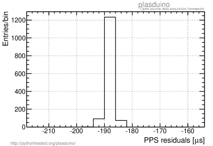
Figure 2: Deviations from the nominal value ($1$ s) of the measured time intervals between two successive 1-PPS pulses from a GPS receiver. The measurement was performed in a climatic chamber with the temperature maintained at $31.8\pm 0.1~{}^{\circ}$C. The mean value of the histogram corresponds to an absolute time accuracy of $\sim 1.9\times 10^{-4}$ and its standard deviation is $1.39~{}\mu$s, close to the nominal time resolution of the system.

For completeness figure 2 shows the distribution of the measured time deviations for a fixed temperature. The root mean square of the histogram bins ($1.39~{}\mu$s) is comparable to the nominal time resolution of the system.

Though we have not performed systematic studies on a large sample of boards, we regard the figures quoted in this section as representative of the typical uncertainties. Without any specific calibration effort the system provides an uncertainty on the absolute time scale of a few parts in $10^{4}$ and a time resolution of the order of a few tens of $\mu$s or better (conservatively assuming that the ambient temperature is controlled to a few ^∘C during the measurements).

3.2 Temperature measurements

We briefly discuss temperature measurements as a typical use case for the Arduino analog inputs. In this case the overall performance depends on the sensor in use; here and in the following, for the sake of discussion, we shall take as an example the NXFT15XH103FA2B, a $10$ k$\Omega$ negative temperature coefficient thermistor readily available for (much) less than 1 € that we routinely use in our didactic laboratories.

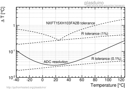
Figure 3: Contributions to the temperature measurement error in our reference setup (a NXFT15XH103FA2B thermistor with a $10$ k$\Omega$ resistor in series). The stochastic term from the ADC resolution typically determines the differential accuracy. Being highly positively correlated, the other contributions only affect the overall absolute temperature scale, i.e., in a limited temperature range they produce a rigid vertical shift.

The thermistor is used in conjunction with a $10$ k$\Omega$ resistor to build a voltage divider whose output voltage is fed into one of the Arduino analog inputs. Given the $R$-$T$ characteristic of the sensor, a 10-bit ADC provides a granularity of $\sim 0.1~{}^{\circ}$C (corresponding to a resolution of $\sim 0.03~{}^{\circ}$C) between $0~{}^{\circ}$C and $40~{}^{\circ}$C (see figure 3). As we shall see in section 4.3 this type of differential resolution is indeed achievable in real-life applications over reasonably narrow temperature ranges.

The systematic uncertainty in the absolute temperature scale is dictated by several different aspects, among which are the linearity of the ADC, the tolerance of the auxiliary resistor (a $0.1\%$ component translates into a typical uncertainty smaller than $0.03~{}^{\circ}$C, constituting a good compromise between price and performance) and the deviation of the sensor response from the nominal characteristic (typically of the order of $0.5~{}^{\circ}$C or less). Figure 3 shows that an overall absolute accuracy below $1~{}^{\circ}$C can be easily achieved with our setup.

3.3 Rate capability

For most of our applications we transfer each single event (e.g., a timestamp or an analog readout) individually to the host computer as soon as the measurement is acquired, as this approach provides the maximal flexibility downstream in terms of monitoring the progress of the data acquisition. In this event-based operation mode the available bandwidth for the serial communication is typically the limiting factor.

Assuming, for the sake of discussion, an event size of $8$–$10$ bytes (e.g., $1$ byte for a control header, $1$ byte for the digital/analog pin number, $4$ bytes for the timestamp, and, optionally, $2$ bytes for an ADC reading, in addition to a $2$ bits per byte overhead due to the start and stop bits of the serial protocol) one saturates the maximum $115200$ baud rate of the Arduino interface at about $1.5$–$2$ kHz. Indeed, the system has proven to run stable with a $\sim 2$ kHz square wave from an external pulse generator fed into a digital input. For applications involving multiple analog inputs one should keep in mind that they are multiplexed on a single ADC so care must be taken to ensure that the signal at the ADC input has enough time to settle.

We note, in passing, that if one is interested in operating the system in counting mode (i.e., accumulating the number of counts into an internal register for a fixed amount of time and transferring the value synchronously), it is easily possible to achieve rates in excess of $10$ kHz.

4 A few real-life applications

In order to illustrate the potential of the system, in this section we describe in detail a couple of specific educational experiments.

4.1 The “digital” pendulum

This experiment involves the use of an optical gate to study the period of a pendulum as a function of time and/or oscillation amplitude. The discriminated output from the optical gate is fed into an Arduino digital input where each signal edge triggers an interrupt sending the timestamp to the host PC. At the end of the acquisition session the data are post-processed into an ASCII file for further analysis.

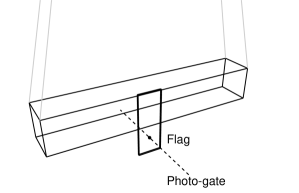
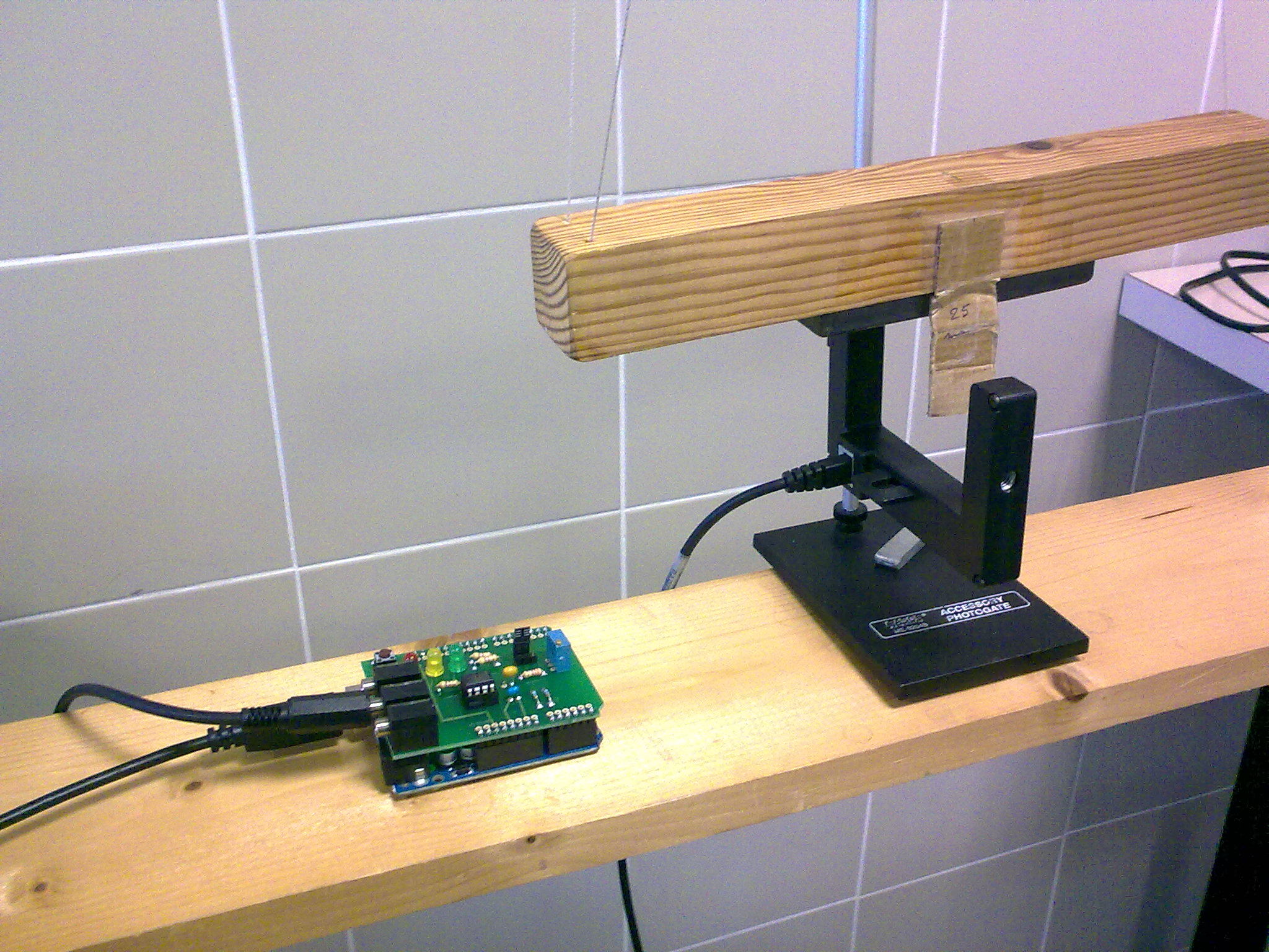
Figure 4: Schematic view (of the left) and picture (on the right) of our digital pendulum setup. The Plasduino hardware (the Arduino board with an interface shield) is also shown in the picture. In order to stabilize the oscillation plane, the pendulum is suspended with four strings. A small flag attached to its body and passing through an optical gate allows to measure the period and the velocity at the bottom of the oscillation.

Figure 4 shows a schematic representation of the basic setup. In order to stabilize the oscillation plane, the pendulum is supported by four strings. The measurement of the transit time of a small flag attached to its body allows to recover the velocity of the center of mass at the bottom of the oscillation—and, therefore, the total mechanical energy. Since the $Q$ factor of the system is reasonably large (typically $500$–$1000$), to first order one can estimate the oscillation amplitude by imposing the conservation of energy:

$$\theta=2\arcsin\left(\frac{k}{T_{t}}\right)\quad{\rm with}\quad k=\left(\frac{w}{2d}\sqrt{\frac{l}{g}}\right),$$ (1)

where $w$ is the width of the flag, $T_{t}$ the measured transit time, $l$ the length of the pendulum (i.e., the distance between the suspension axis and the center of mass) and $d$ the distance between the suspension axis and the light beam from the photogate.

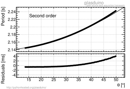
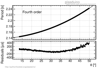
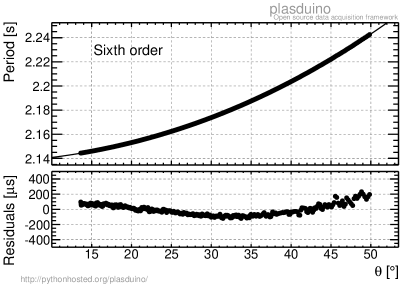
Figure 5: Anharmonicity study with our digital pendulum setup. The measured period is plotted as a function of the oscillation amplitude—estimated from eq. (1)—and fitted with the Taylor expansion in eq. (2), truncated at second, fourth and sixth order. In each of the three case only the multiplicative constant $T_{0}$ is left free to float in the fit. Note the different y-axis scales for the residual plots.

Figure 5 shows an illustrative example of anharmonicity study. The measured period is plotted against the oscillation amplitude estimated from eq. (1) and fitted with the Taylor expansion [7] of the period itself:

$$T=T_{0}\left(1+\frac{1}{16}\theta^{2}+\frac{11}{3072}\theta^{4}+\frac{173}{737280}\theta^{6}+\frac{22931}{1321205760}\theta^{8}+\cdots\right),$$ (2)

truncated at different orders (note that in every case only $T_{0}$ is left free in the fit, while all the coefficients of $\theta^{n}$ are fixed to their nominal values). For reference, at $50^{\circ}$ the relative weight of the $\theta^{4}$ term, from eq. (2), is $\sim 2.1\times 10^{-4}$ (or $\sim 4$ ms for a $\sim 2$ s period) while that of the $\theta^{6}$ term is $\sim 1.0\times 10^{-4}$ (or $\sim 200~{}\mu$s for a $\sim 2$ s period). These figures are in reasonable agreement with the results shown in figure 5, though it is clear that the model in eq. (1) is too rough to reproduce the richness of the data, as systematic residuals at the level of $\sim 100~{}\mu$s are present the fit with the eq. (5) truncated at the sixth order.

4.2 The “analog” pendulum

This is a variation on the theme where we use a small plastic container filled with demineralized water as a voltage divider for a real-time tracking of the motion of a pendulum. As shown in figure 6, the container features two metal plates (one on each of the two ends) connected to the ground and $V_{\rm cc}$ voltage references provided by the Arduino board. The tip of the pendulum is immersed in the water and connected to one of the analog inputs of the board itself so that—non linearity and geometrical projective effects aside—the voltage at the pin is proportional to the position of the pendulum.

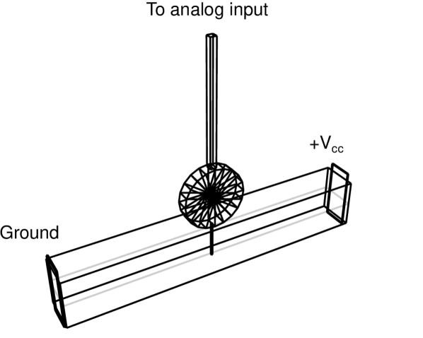
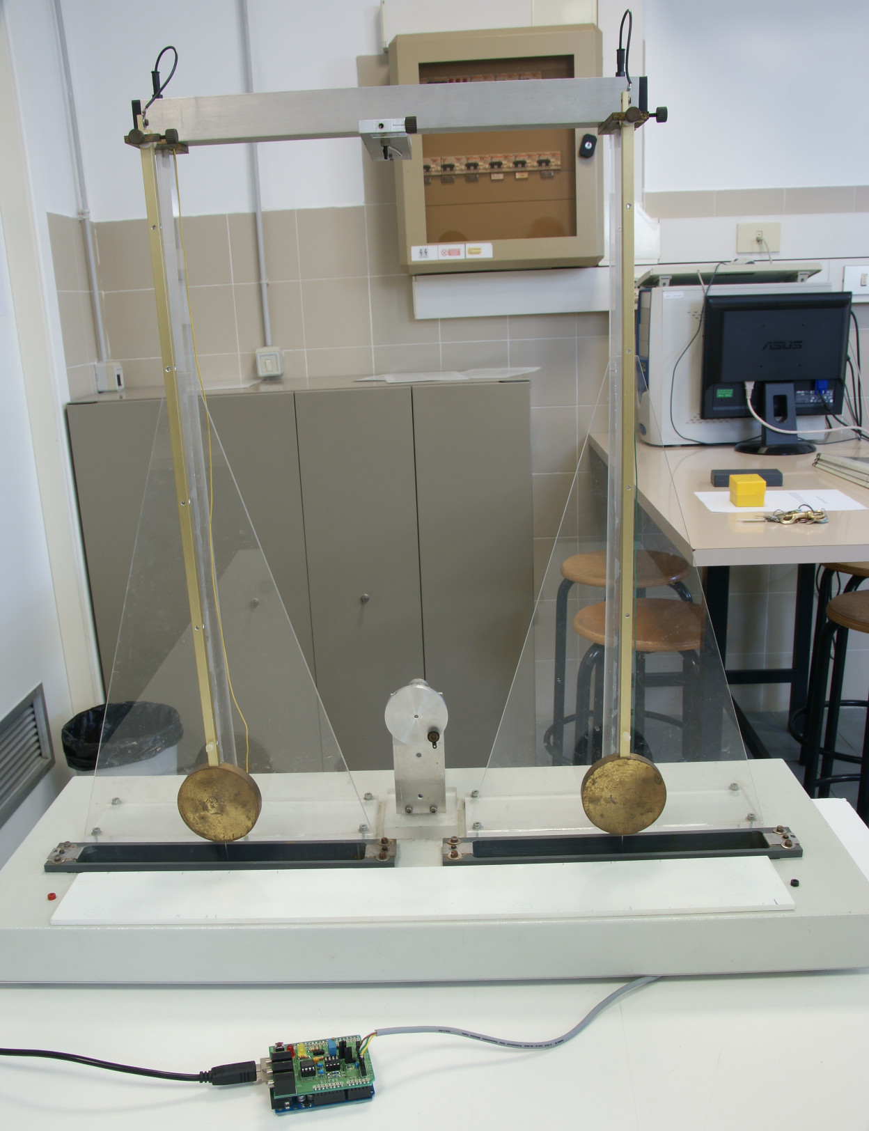
Figure 6: Schematic view (above) and picture (on the right) of our analog pendulum setup. The water container and the pendulum tip, together, act as a voltage divider allowing to track in real time the position of the tip itself. For reference, the dimensions of the container are $43.0\times 5.0\times 4.5$ cm³.

With a $10$ bit ADC and a maximum excursion of $\sim 40$ cm a theoretical granularity of $40/2^{10}$ cm (or $400~{}\mu$m) can be achieved—and a corresponding spatial resolution of $400/\sqrt{12}\sim 115~{}\mu$m. It is quite remarkable, in fact, how such a simple setup allows to easily achieve a sub-mm position resolution.

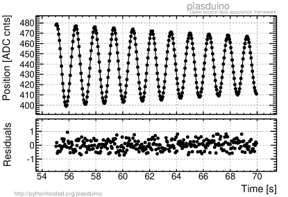
Figure 7: Typical example of real-time pendulum tracking. A fit with eq. (3) assuming the nominal $1/\sqrt{12}$ ADC counts as $1$-$\sigma$ errors on the position measurements yields a $\chi^{2}$ of $457.4/293$, indicating that the position resolution (at least in the $\sim 3.5$ cm range shown here) is only slightly ($\sim 25\%$) worse than the theoretical limit. Note that the errors on the data points and on the residuals are omitted for visualization purposes.

Figure 7 shows a sample data acquisition, with the experimental points fitted with the function

$$x(t)=c_{0}+c_{1}e^{-\lambda t}\sin(\omega_{0}t+\phi_{0}).$$ (3)

The root mean square of the residuals is $\sim 0.36$ ADC counts, which is only $25\%$ larger that the nominal $1/\sqrt{12}$ value one would obtain if the system noise and non-linearity were negligible. (We stress, however, that non linearities at the level of a few %, that can possibly be handled with a dedicated calibration, are observed at the edges of the container.)

The setup illustrated in figure 6 can be easily modified as to include a small motorized aluminum wheel with a fixed pin connected to the body of the pendulum through a pair of springs and acting as a(n approximately) sinusoidal external force. The speed of the motor (and hence the frequency of the input load) can be controlled by means of the Arduino PWM capabilities (and, assuming that the apparatus is properly sized, the current provided by a standard USB port is enough to drive the motor and no external power supply is required).

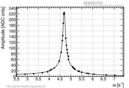
Figure 8: Resonance curve of a pendulum driven by an external sinusoidal force, produced using a slightly modified version of the setup illustrated in figure 6. The data points are fitted with the function in eq. (4). We note that no attempt has been made to calibrate the non linearity of the system.

This modified setup allows to study the steady-state oscillation amplitude of the pendulum as a function of the angular pulsation of the external force, producing a resonance curve of the system. Figure 8 shows how, even with no attempt at calibrating the non linearities, the system response is in remarkable agreement with the prediction of the simplest possible model (i.e., with a single friction term proportional to the velocity):

$$A(\omega)=\frac{A_{0}}{(\omega_{0}^{2}-\omega^{2})^{2}+4\Gamma^{2}\omega^{2}}.$$ (4)

4.3 Measurement of thermal conductivity

We illustrate this thermodynamics experiment as a last illustrative example of the capabilities of the system. The setup is as simple as a metal bar with a regular set of holes allowing to measure the temperature profile as a function of the position along the bar itself. The temperatures on the two ends of the bar are set by a resistor heated up due to Joule effect and a steady flow of running fresh water, respectively. The left panel of figure 9 shows the apparatus, with two bars of different material available. The plasduino board is also visible with two thermistors connected. One thermistor is placed in the first hole of one bar, while the other is left floating to measure air temperature. Neglecting the heat exchanges with the ambient (which can be minimized by ensuring that the temperature of any point in the bar is not too different from the ambient temperature), the theory predicts the temperature profile to be linear

$$T(x)=T_{0}-\frac{W}{\lambda S}x$$ (5)

(here $W$ is the power provided by the voltage supply driving the resistor, $S$ is the cross section of the bar and $\lambda$ the thermal conductivity of the material). Moving the thermistor from one hole to the other, the temperature profile can be measured, as shown in the right panel of figure 9, and its slope allows to estimate $\lambda$.

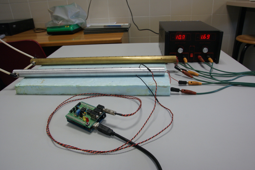
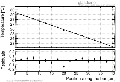
Figure 9: On the left, the picture of the apparatus showing also the plasduino system connected with the two thermistors. On the right, the temperature profile of a metal bar kept at constant (different) temperatures at its extremes. A linear fit assuming that the measurement errors are solely dictated by the ADC resolution (i.e., $\sim 0.03~{}^{\circ}$C) yields a $\chi^{2}$ of $35.9/13$, possibly indicating that the errors themselves are slightly underestimated. For reference, the relative uncertainty on the fitted slope is $\sim 0.5\%$.

4.4 Displaying data in real time

Admittedly, Plasduino is designed as a data acquisition system—i.e. emphasis is put on the two basic tasks of (i) collecting data and (ii) storing them in a suitable form for off-line analysis. That being said, we fully realize the educational value of being able to display data in real time and provide a set of interactive graphical widgets for the purpose, which are used in some of the modules, as shown in figure 10. There is no doubt this is one of the aspects where the system could be improved, partially evolving toward an on-line learning platform.

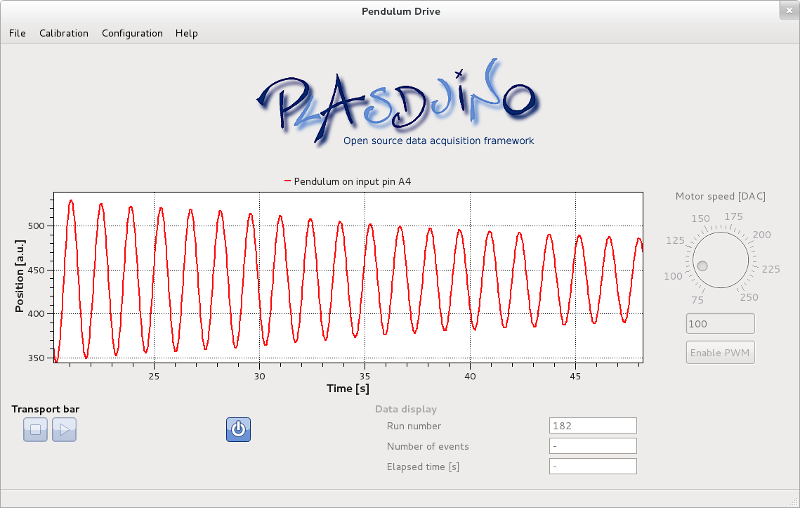
Figure 10: Graphical user interface for the analog pendulum setup described in section 4.2. The canvas displaying the time series can be used interactively and allows to perform the basic analysis previously described with the computer mouse—without any post-processing of the data.

5 Status and prospects

The Plasduino framework has been in use in the didactic laboratories of the Physics Department of the University of Pisa for more than two years, now, in the form of a set of seven educational experiments that we routinely propose to undergraduate and high-school students—i.e., students with no data acquisition experience and facing basic data analysis for the first time. The graphical user interface, and the system in general, proved to be intuitive enough to be effectively used by novices with little or no need for very specific instructions. As a matter of fact, we have produced a number of fully-assembled systems which are currently in use in the didactic laboratories of a few local high schools and we have agreements with other schools to continue working in this direction.

We strive for making available in a terse form all the information necessary to replicate the system (electronics schematics, part lists, cable and connector layouts, software installation instructions) and we sustain that this can be realistically achieved by anybody with basic computer skills and some soldering experience (e.g., many of the high-school technicians we interacted with during the development). It goes without saying that actively developing the system in any of its parts requires skills that go well beyond those mentioned in the previous paragraph.

In the near term we are working on the implementation of a few more advanced educational modules, most notably a configurable waveform generator and a data acquisition shield to read signals from photomultiplier tubes (integrating a GPS receiver for the absolute timestamp). In parallel, we started a collaboration with a local high school to assemble a fully fledged weather station.

- [1] http://pythonhosted.org/plasduino/
- [2] http://www.arduino.cc/
- [3] http://www.python.org/
- [4] http://www.riverbankcomputing.com/software/pyqt/intro
- [5] http://www.udoo.org/
- [6] http://pythonhosted.org/plasduino/screenshots.html
- [7] \BYNelson R. A. \atqueOlsson M. G. \INAmerican Journal of Physics54 (2)1985112–121