Visualizing genetic constraints

Abstract

Principal Components Analysis (PCA) is a common way to study the sources of variation in a high-dimensional data set. Typically, the leading principal components are used to understand the variation in the data or to reduce the dimension of the data for subsequent analysis. The remaining principal components are ignored since they explain little of the variation in the data. However, evolutionary biologists gain important insights from these low variation directions. Specifically, they are interested in directions of low genetic variability that are biologically interpretable. These directions are called genetic constraints and indicate directions in which a trait cannot evolve through selection. Here, we propose studying the subspace spanned by low variance principal components by determining vectors in this subspace that are simplest. Our method and accompanying graphical displays enhance the biologist’s ability to visualize the subspace and identify interpretable directions of low genetic variability that align with simple directions.

, , , , ,
and

t5Supported by National Science Foundation EF-0328594.

t6Supported by National Science Foundation IOS-061179.

t2Supported by the National Science and Engineering Research Council of Canada.

4Supported by National Science Foundation Grant DEB-0819901.

t3Supported by National Science Foundation Grant DEB-0129018.

t7Supported by NSF Grants DMS-03-08331 and DMS-06-06577.

1 Introduction

Evolutionary biologists study how the distribution of observable characteristics of individuals in a population changes over generations. These observable characteristics are called traits or phenotypes and can be qualitative, such as body color in a specific environment, or quantitative. A quantitative phenotype can be a scalar such as mass at a specified age, or a vector such as mass at several specified ages, or a function such as mass at a continuum of ages.

Changes in the distribution of traits can occur via many processes, including mutation, selection and genetic drift (the change in the distribution of genotypes that can occur in a finite population when mating and reproduction are modeled as random processes). Here we consider changes caused by selection. We consider changes within only one generation. We characterize changes by the expected change in phenotype, and we assume that the population under selection is, in essence, infinite. The selection process determines which individuals in a population are likely to produce viable offspring. Selection can occur naturally, when, for instance, small individuals are more vulnerable to predation, or artificially, as in the selective breeding of race horses. Selection causes the trait distribution of the subpopulation of breeding individuals to differ from that of the original population. This difference will persist into the offspring population provided the trait has some genetic component.

To understand the role of selection and genetics in evolution, consider the following simple example. Suppose that, in a population, individuals taller than a certain height do not reproduce. Thus, the breeding subpopulation will have a smaller mean height than the original population. The breeding parents’ offspring also will have a smaller mean height provided height has some genetic basis. In this case, we say that selection on height leads to the evolution of height.

Thus, evolution requires both a selection process and a genetic component. The selection process must involve a trait with a genetic component. That genetic component must differ between breeding and nonbreeding individuals.

Clearly, genetic variation plays an important role in evolution. As we will see, the amount of genetic variation actually determines the speed at which selection causes evolutionary change. In nature, traits with substantial genetic variation will respond rapidly, allowing the species to adapt rapidly to changing conditions. Genetic variation is likewise a critical variable for plants and animals that are used in agriculture. Artificial selection (or selective breeding) has been used for millennia to improve domesticated species, and it continues to be one of the most important tools for increasing agricultural yield. The amount of genetic variation present is one of the key criteria used by animal and plant breeders to choose the traits for artificial selection. In both natural and domesticated populations, traits with little or no genetic variation are not able to respond much or at all to selection. These traits are said to be genetically constrained, and these constraints play an important role in determining how populations adapt [see Kirkpatrick and Lofsvold (1992)].

In this paper we propose methods to explore genetic constraints in vector-valued traits. The next section contains biology background, including a model for selection and a characterization of genetic constraints as eigenvectors of the genetic covariance matrix corresponding to zero eigenvalues. Sections 3 and 4 describe our proposed methodology for studying genetic constraints. Data analyses appear in Section 5 and a simulation study in Section 6.

2 Biology background

Biologists model an individual’s quantitative trait in terms of components, the simplest model involving two components: a genetic component, $g$, inherited from parents, and an environmental component, $e$, such as availability of food. In this simple model, the true phenotype is $g+e$ and the observed phenotype, $y$, is

$$y=g+e+\varepsilon,$$

where $\varepsilon$ is additional sampling variation. We denote the expected value of $g$ by $\mu$ and its variance/covariance by $\mathcal{G}$. If $g$ is scalar, then $\mathcal{G}$ is its variance. If $g$ is a vector of length $K$, then $\mathcal{G}$ is the $K$ by $K$ covariance matrix with $ij$th entry equal to the covariance between the $j$th and $k$th component of $g$. If $g$ is a function, say, if $g(t)$ is mass at age $t$, then $\mathcal{G}$ is a bivariate function, with $\mathcal{G}(s,t)$ being the covariance between mass at age $s$ and mass at age $t$. The environmental effect $e$ is a mean zero random component with variance/covariance $\mathcal{E}$, with $\mathcal{E}$ defined in an analogous way as $\mathcal{G}$. The random components $g$, $e$ and $\varepsilon$ are defined so as to be uncorrelated, so the covariance of the true phenotype is $\mathcal{G}+\mathcal{E}$ and the covariance of the observed phenotype is $\mathcal{G}+\mathcal{E}$ plus the variance/covariance of $\varepsilon$. The marginal distributions of $g$ and $e$ are population and generation dependent, while the marginal distribution of $\varepsilon$ depends on the method of measuring the phenotypes.

The heritability of a scalar phenotype is the proportion of its variance that is attributable to genetics, that is, the heritability is simply $h^{2}=\mathcal{G}/(\mathcal{G}+\mathcal{E})$. Throughout, we assume that $[\mathcal{G}+\mathcal{E}]^{-1}$ exists. To understand the role of heritability in evolution, consider our simple example where the selection mechanism prevents tall individuals from producing offspring. First suppose that height has zero heritability in the population, that is, all variability in height is simply due to environmental effects. Then, intuitively, the distribution of heights in the next generation will be the same as the distribution in the original population, provided both generations are raised in similar environments. However, if height has nonzero heritability, that is, if the genetic component of height varies across individuals, then the distribution of heights in the next generation will be different from the distribution in the original population. One would expect that the larger the heritability in the original population, the bigger the change in the distribution of heights in the next generation.

The mathematical theory that supports this reasoning, that links heritability and evolution of a trait from one generation to the next, is contained in the Breeder’s equation. To define this equation, let $\mu_{p}$ be the expected phenotype in the original population, $\mu_{p^{*}}$ the expected phenotype of the reproducing adults, and $\mu_{o}$ the expected phenotype of their offspring. The Breeder’s equation gives $\mu_{o}-\mu_{p}$, the expected response to selection:

$$\mu_{o}-\mu_{p}={\mathcal{G}}[\mathcal{G}+\mathcal{E}]^{-1}\times(\mu_{p^{*}}-\mu_{p}).$$ (1)

In our height example, $\mu_{p^{*}}$ is less than $\mu_{p}$ and so the Breeder’s equation tells us that the mean height in the offspring population is less than or equal to that in the original population. How much less depends on the value of the heritability ($h^{2}={\mathcal{G}}[\mathcal{G}+\mathcal{E}]^{-1}$) and the strength of selection. The strength of selection determines if particular individuals will reproduce. In our simple height example, the strength of selection is determined by the height cutoff for reproducing. Thus, the strength of selection determines $\mu_{p^{*}}-\mu_{p}$. Biologists define the selection differential as $s=\mu_{p^{*}}-\mu_{p}$. The Breeder’s equation also holds for multivariate phenotypes, where, if the phenotype is a vector of $K$ values, then $\mu_{o},\mu_{p}$ and $\mu_{p^{*}}$ are $K$-vectors and $\mathcal{G}$ and $\mathcal{E}$ are $K\times K$ covariance matrices. For a generalization of the Breeder’s equation to function-valued traits, see Kirkpatrick and Heckman (1989).

Biologists rewrite the Breeder’s equation in terms of the selection gradient, denoted $\beta$. The selection gradient is defined in terms of a population’s expected fitness, that is, its ability to reproduce, under the specified selection mechanism. We can think of the selection gradient as the change in $\mu_{p}$ that selection appears to be making when “choosing” the breeding individuals in the original population. This is not, in general, equal to $s=\mu_{p^{*}}-\mu_{p}$, the change that actually occurs. To see the distinction between $\beta$ and $s$, consider once again our simple height example, but suppose that the phenotype is a vector in $\Re^{2}$ with components height and weight. Selection is only acting on height, not on weight, so the selection gradient’s second component is zero. However, the second component in $s$ is not 0 since height and weight are positively correlated: the selection on height means that both the heights and weights of the reproducing individuals will, on average, be smaller than those in the original population. One can show that the selection gradient $\beta$ and the selection differential $s$ are related via the equation $s=[\mathcal{G}+\mathcal{E}]\beta$. This yields an alternative expression for the expected response to selection in the Breeder’s equation in (1):

$$\mu_{o}-\mu_{p}={\mathcal{G}}\beta.$$ (2)

We consider the amount of genetic variation explained by the direction of a unit vector $v$. This amount of variation is the magnitude of ${\mathcal{G}}v$, that is, the magnitude of the expected response to selection when $v$ is the selection gradient.

For more details on the Breeder’s equation, the selection gradient and the selection differential, see Lande (1976, 1979), Lande and Arnold (1983) or, for a statistician-friendly exposition, Heckman (2003). For an extension of (2) to function-valued traits, see Gomulkiewicz and Beder (1996) and Beder and Gomulkiewicz (1998).

From (2), we can see the importance of an eigenanalysis of $\mathcal{G}$ in understanding a population’s ability to evolve under selection. The magnitude of $\mu_{o}-\mu_{p}$ will be largest when the selection gradient, $\beta$, points in the same direction as the leading eigenvector of $\mathcal{G}$. The value of $\mu_{o}-\mu_{p}$ will be zero if selection acts in the direction corresponding to a zero eigenvalue of $\mathcal{G}$. That is, the population’s mean phenotype will not evolve if selection acts in the direction of an eigenvector of $\mathcal{G}$ corresponding to a zero eigenvalue. These directions are called genetic constraints. Eigenvectors corresponding to small but nonzero eigenvalues are also of interest. Gomulkiewicz and Houle (2009) provide tools to determine what eigenvalues are considered small: they model demography and evolution in a population experiencing selection due to changing environmental conditions. They identify critical levels of genetic variability, levels low enough to effectively prevent the adaptive evolution that might result from selection.

3 Analysis of genetic variability

To better understand the directions of genetic variability, we partition the sample space of $g$ into two subspaces, the model space and the nearly null space. The model space is a “high genetic variance” subspace spanned by eigenvectors of ${\mathcal{G}}$ with large eigenvalues. The nearly null space is the orthogonal complementary “low genetic variance” subspace. Visualizing the nearly null space provides information about the existence and interpretation of genetic constraints. This partitioning and the associated visualization tools were introduced in Gaydos (2008).

To explicitly define the model space and the nearly null space of a covariance matrix $\mathcal{G}$, let $\lambda_{1}\geq\lambda_{2}\geq\lambda_{3}\geq\cdots$ be the eigenvalues of $\mathcal{G}$, and $v_{1},v_{2},v_{3},\ldots$ the corresponding orthonormal eigenvectors. We decide which $\lambda_{k}$’s to consider as large values, say, $\lambda_{1},\ldots,\lambda_{J}$, and assume that $\lambda_{J}$ is strictly greater than $\lambda_{J+1}$. We define the model space as the space spanned by $v_{1},v_{2},\ldots,v_{J}$ and the nearly null space as the space spanned by the remaining eigenvectors. From the Breeder’s equation (2), we see that $\mu_{o}-\mu_{p}$ is large if $\beta$ lies in the model space. Specifically, for $\beta$ in the model space, $\|\mu_{o}-\mu_{p}\|/\|\beta\|\geq\lambda_{J}$ and is largest when $\beta$ is a constant times $v_{1}$. Conversely, if $\beta$ lies in the nearly null space, then $\|\mu_{o}-\mu_{p}\|$ will never exceed $\lambda_{J+1}\|\beta\|$.

Interpreting the nearly null space is challenging since, typically, eigenvectors corresponding to small eigenvalues are “rough” and may simply represent noise. To study the nearly null space, we construct a new basis for this space, ordered by simplicity. If the simplest basis vectors are interpretable, biologists can then study the possibility of genetic constraints. If the simplest basis vectors are not interpretable, then biologists might consider the nearly null space to represent noise.

Clearly, the choice of $J$ is important in the definition of the model space and nearly null space. One might carry out a sequence of hypothesis tests to choose $J$, using the procedures of Amemiya, Anderson and Lewis (1990), Anderson and Amemiya (1991) or Hine and Blows (2006). These authors consider testing for the dimension of $\mathcal{G}$ when data come from a half-sibling design, that is, where data are from independent families and each family consists of half-siblings. Such data can be modeled as an easy-to-analyze multivariate one-way classification with random effects [Lynch and Walsh (1998)]. Hypothesis testing to determine $J$ in more complicated designs might be challenging. However, we do not recommend this hypothesis testing approach, preferring instead an exploratory approach grounded in the biology. We recommend the usual techniques of calculating the proportion of genetic variance explained, studying scree plots and considering the interpretability of the associated eigenvectors, combined with the calculations of critical levels as defined in Gomulkiewicz and Houle (2009). We also recommend that subject area specialists examine results for a range of values of $J$, to examine the interplay between proportion of variance explained and biological interpretability of the resulting model space and nearly null space. These subject area opinions can provide a more biologically meaningful and thus more compelling explanation of a choice of reasonable values of $J$ than any test of significance or other algorithmic approach. In addition, studying a range of values of $J$ allows the user to consider small-scale and large-scale genetic variabilities.

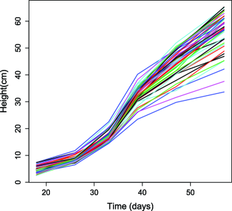
Figure 1: Heights of 49 jewelweed plants raised in sun in a dense environment. The heights are measured at six times and linearly interpolated. See Stinchcombe et al. (2010) for details of the experiment.

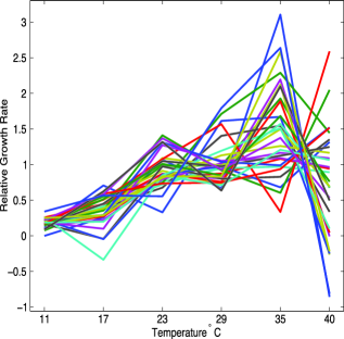
Figure 2: Relative growth rates of the caterpillar Pieris rapae as a function of temperature. The growth rates, in milligrams per hour, are measured at six temperatures and linearly interpolated. See Kingsolver, Ragland and Shlichta (2004) for details of the experiment.

In summary, we use principal components analysis and simplicity measures to define biologically interpretable directions of low genetic variation, allowing biologists to explore the possibility of the existence of genetic constraints. We apply our method to two data sets, one of the heights of jewelweed plants (Impatiens capensis) measured at six ages, the other of growth rate measurements of the caterpillar Pieris rapae at six temperatures. The jewelweed data are described in Stinchcombe et al. (2010) and the caterpillar data in Kingsolver, Ragland and Shlichta (2004). The two data sets are displayed in Figures 1 and 2. Descriptions of the data and the purpose of the experiments, along with data analysis and discussion, are given in Section 5.

4 Simplicity basis

A simplicity basis for a linear subspace $\mathcal{V}$ of $\Re^{K}$ is an orthonormal basis $\{w_{1},\ldots,w_{L}\}$, where the $w_{k}$’s are ordered according to some simplicity measure: $w_{1}$ is the “simplest” element of unit length in $\mathcal{V}$, $w_{2}$ is the “simplest” unit-length element of ${\mathcal{V}}$ that is orthonormal to $w_{1}$, $w_{3}$ is the “simplest” unit-length element of ${\mathcal{V}}$ that is orthonormal to $w_{1}$ and $w_{2}$, and so forth. Such a basis may help us to understand $\mathcal{V}$ since simple vectors are usually the most interpretable.

We consider quadratic simplicity measures, that is, measures equal to $v^{\prime}\Lambda v$. We assume throughout that $\Lambda$ is a nonnegative definite symmetric matrix and, for interpretability, that $\Lambda$ is defined so that the simpler the vector the higher the simplicity score. If this is not the case, that is, if $v^{\prime}\Lambda v$ is small when $v$ is simple, we can instead use the simplicity measure $v^{\prime}(\lambda{\mathrm{I}}-\Lambda)v$, where I is the identity matrix and $\lambda$ is some number greater than or equal to the largest eigenvalue of $\Lambda$. Examples of quadratic simplicity measures can be found in smoothing and penalized regression. See, for instance, Eilers and Marx (1996) or Green and Silverman (1994). In the examples that follow, we think of the elements of a vector $v$ as evaluations of a function $f$: $v=({\mathrm{v}}_{1},\ldots,{\mathrm{v}}_{K})^{\prime}=(f(t_{1}),\ldots,f(t_{K}))^{\prime}$. In these examples, we used a simplicity measure based on first divided differences:

$$\sum_{j}\frac{({\mathrm{v}}_{j}-{\mathrm{v}}_{j-1})^{2}}{(t_{j}-t_{j-1})},$$

which is a good approximation of $\int(f^{\prime})^{2}$. To transform this to a measure that is large for simple $v$’s, we use the result of Schatzman (2002) that $\sum({\mathrm{v}}_{j}-{\mathrm{v}}_{j-1})^{2}\leq 4\sum{\mathrm{v}}_{j}^{2}$ for all $v$’s. Our simplicity measure is equal to

$$4v^{\prime}v-\min_{j}\{t_{j}-t_{j-1}\}\times\sum\frac{({\mathrm{v}}_{j}-{\mathrm{v}}_{j-1})^{2}}{(t_{j}-t_{j-1})},$$ (3)

which lies between 0 and 4 inclusive. The simplicity measure (3) is just one of many possible smoothing-based measures. Another good choice might be the measure used in cubic smoothing spline regression, where a function $f$’s simplicity is defined as $\int(f^{\prime\prime})^{2}$, with a low value signifying simplicity. This integral can be approximated using a Rieman sum of second divided differences, yielding a quadratic form in $(f(t_{1}),\ldots,f(t_{n}))^{\prime}$.

The simplicity basis of the subspace $\mathcal{V}$ for the simplicity measure associated with a nonnegative definite symmetric matrix $\Lambda$ is easy to calculate. Let $v_{1},\ldots,v_{L}$ be an orthonormal basis of $\mathcal{V}$ and let $P$ be the $K\times L$ matrix with $k$th column equal to $v_{k}$. So $P$ is a projection matrix onto ${\mathcal{V}}$. Let $\alpha_{1},\ldots,\alpha_{L}$ be the eigenvectors of $P^{\prime}\Lambda P$ with corresponding eigenvalues $\lambda_{1}\geq\lambda_{2}\geq\cdots\geq\lambda_{L}$. Then it is straightforward to show that $\{P\alpha_{1},\ldots,P\alpha_{L}\}$ is a simplicity basis of $\mathcal{V}$, ordered from most simple to least simple. When the eigenvalues are distinct, the basis is unique, not dependent on the choice of $P$. However, if, for example, $\lambda_{1}=\lambda_{2}>\lambda_{3}$, then the “simplest subspace” of $\mathcal{V}$ is the span of $P\alpha_{1}$ and $P\alpha_{2}$, and this subspace does not depend on the $P$ that we choose.

5 Data analysis

For well-designed evolutionary biology studies such as those presented here, the covariance matrix ${\mathcal{G}}$ is identifiable, estimable and consistent. Typical methods of estimation are via MANOVA, maximum likelihood or restricted maximum likelihood (REML). See, for instance, Searle, Casella and McCulloch (2006) and Lynch and Walsh (1998). These estimates take into account the dependence in the data caused by individuals’ relatedness.

For each data set, we carry out a principal components analysis of the estimate of $\mathcal{G}$ and, for all possible values of $J$, we study the model space of dimension $J$ and the corresponding nearly null space. For our data sets, $J$ ranges from 0 to 6. The supplementary material for this paper contains all seven plots of the caterpillar analysis and all seven plots of the jewelweed analysis. Here, we present just two of the seven plots for each data set.

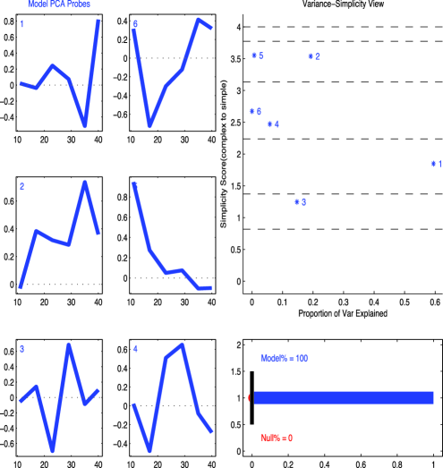
Figure 3: Caterpillar data: PCA basis. The vectors in the left panel are the six principal components vectors of the estimated genetic covariance matrix. These vectors explain 100% of the genetic variance, as indicated in the lower right plot. The upper right plot shows each vector’s simplicity score and the percent of genetic variance it explains. The amounts of genetic variance explained by vectors 1 through 6 are, respectively, 0.618, 0.200, 0.153, 0.061, 0.008, 0.

The details and interpretations of Figures 3 through 6 are in Sections 5.1 and 5.2, but we provide an overview here. Figures 3 and 5 show the principal component vectors for the two data sets, corresponding to choosing $J=6$, for a six-dimensional model space and a zero-dimensional nearly null space. These figures are shown so we can contrast insight from a usual PC analysis with the insight obtained from Figures 4 and 6. Figure 4 shows the four-dimensional model space and two-dimensional nearly null space for the caterpillar data. Figure 6 shows the two-dimensional model space and four-dimensional nearly null space for the jewelweed data.

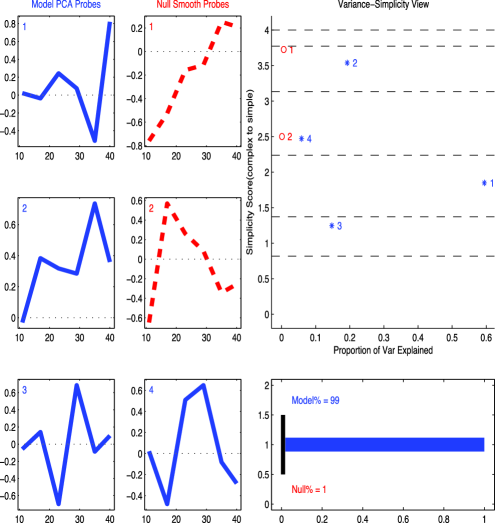
Figure 4: Caterpillar data: two-dimensional nearly null space. The structure of the plot is as in Figure 3 except that the left-hand side shows the PC basis for the four-dimensional model space (blue) and the simplicity basis for the two-dimensional nearly null space (red dashed). The simplest nearly null space vector is labeled with a red 1. The amount of genetic variance explained by the simplest nearly null vector is 0.007 and by the second simplest 0.001.

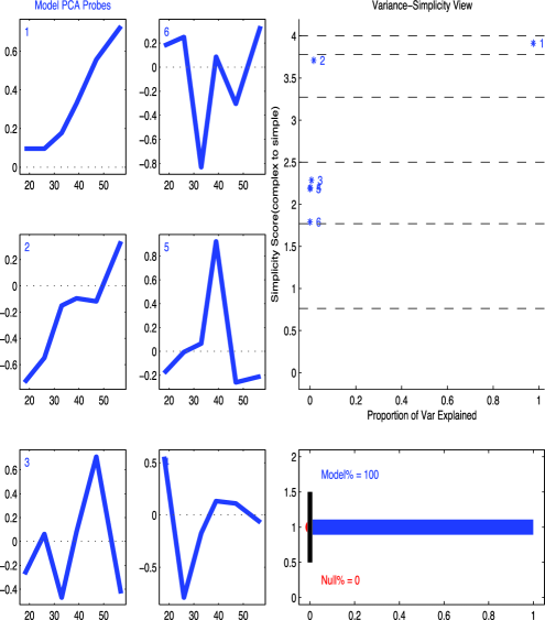
Figure 5: Jewelweed data for height as a function of time in the sun/high density group: PCA basis. The structure of the plot is as in Figure 3. The amounts of genetic variance explained by vectors 1 through 6 are, respectively, 48.98, 0.82, 0.33, 0.08, 0 and 0.

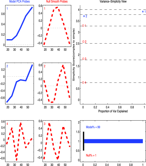
Figure 6: Jewelweed data for height as a function of time in the sun/high density group: four-dimensional nearly null space. The structure of the plot is the same as that of Figure 4. The amounts of genetic variance explained by simplicity vectors 1 through 4 are, respectively, 0.02, 0.22, 0.15 and 0.02.

The six plots in the left sides of Figures 3 through 6 show six orthonormal basis vectors for $\Re^{6}$. The first $J$, in solid blue lines, are the first $J$ principal component vectors, labeled with a blue 1 for the first principal component, a blue 2 for the second principal component, etc. The remaining (6–$J$) basis vectors—the dashed red lines which only appear in Figures 4 and 6—form the simplicity basis for the nearly null space. The simplest basis vector is labeled with a red 1, the next simplest with a red 2, etc. The simplicity measure is that in (3), with large values of the measure being most simple. We have arranged the plots of the six basis vectors so that the top row contains what are arguably the most interesting basis vectors: the eigenvector corresponding to the largest eigenvector and the nearly null space’s simplest vector. Nearly null space vectors are plotted counter-clockwise in order of simplicity, while eigenvectors are plotted clockwise in order of the corresponding eigenvalues.

Each of the six basis vectors, when used as a selection gradient, produces an expected response to selection, as given in equation (2). A natural estimate of the expected response to selection for a selection gradient $\beta$ is simply $\hat{\mathcal{G}}\beta$, where $\hat{\mathcal{G}}$ is the estimate of the genetic covariance matrix. The captions under Figures 3 through 6 list the six vector norms of $\hat{\mathcal{G}}\beta$, one for each of the six basis vectors. Note that, if $\beta$ is a unit-length eigenvector of $\hat{\mathcal{G}}$, then the norm of $\hat{\mathcal{G}}\beta$ is simply equal to the associated eigenvalue. The norm of $\hat{\mathcal{G}}\beta$ is maximal when $\beta$ is the eigenvector associated with the largest eigenvalue of $\hat{\mathcal{G}}$.

The norms of the expected responses to selection can also be reported as proportions of genetic variance, simply by reporting each norm divided by the sum of the norms. These proportions of genetic variance are plotted on the horizontal axes in the upper right panels of Figures 3 through 6, with simplicity scores on the vertical axes. The numbering and color-coding correspond to the plots on the left. The panel in the lower right shows the total genetic variance explained by the model space and by the nearly null space.

5.1 Caterpillar data analysis

Kingsolver, Ragland and Shlichta (2004) estimated genetic variation in short-term growth rates of caterpillars at several temperatures ranging from 11^∘C to 40^∘C. The type of caterpillar was Pieris rapae, which develops into the Small Cabbage White Butterfly. The caterpillars cause extensive damage to crops such as cabbage and broccoli, so understanding their growth is important for commercial agriculture. The goal of the study was to quantify patterns of genetic variation in growth rate across temperatures, and explore how these patterns might affect evolutionary responses to selection in changing temperature conditions in nature. For instance, if there was little genetic variability in growth rates at high temperatures, rising temperatures could cause extinction of Small Cabbage White Butterflies. Alternatively, if growth rate at high temperatures is negatively genetically correlated with growth rate at low temperatures, then rising temperatures could lead to reductions in growth rate at low temperatures.

Caterpillars were reared individually from hatching on artificial diet in diurnally fluctuating conditions of temperature (11–35^∘C) and light (15 hours of light, 9 hours of dark) until the start of the developmental stage known as the 4th larval instar. The studies focused on the 4th instar because more than 85% of all growth occurs during the 4th and 5th instars; measurements were concentrated within a single instar to quantify effects of temperature on larval growth (mass increase) as distinct from development (molting, or the developmental processes involved in the transitions between instars). See Kingsolver, Ragland and Shlichta (2004) for details of the measurements and methods. Briefly, the short-term growth rate of each caterpillar was measured at six different temperatures between 11^∘C and 40^∘C (11, 17, 23, 29, 35 and 40^∘C), during the first two days of the 4th instar (Figure 2). To reflect the natural diurnal cycle typically experienced by caterpillars in nature, measurements at higher temperatures were done during the day (light phase) and at lower temperatures during the night (dark phase); growth rate was calculated as the net change in mass over the measurement period. Because exposure to 40^∘C is potentially stressful and could affect subsequent feeding and growth, measurements at this temperature were done last for each caterpillar. Measurements of 1088 individuals from 90 independent families of full siblings were completed. These data were used to estimate the genetic variance–covariance matrix ${\mathcal{G}}$ for growth rate at the six temperatures, using the REML software dfreml described by Meyer and Smith (1996).

To study the nearly null space, we define simplicity via (3) with $t_{j}-t_{j-1}=6$ for $j=2,\ldots,5$ and $t_{6}-t_{5}=5$.

Figure 3 shows the principal components decomposition (six-dimensional model space, 0-dimensional null space) of the matrix ${\mathcal{G}}$. The first PC, explaining 59.5% of the variation, is dominated by strong loadings of opposite sign for growth rate at 35^∘C and 40^∘C, reflecting the strong negative genetic covariance between growth at these two temperatures. This first PC has a low simplicity score. In contrast, the second PC has a much higher simplicity score and reflects loadings of the same sign and similar magnitude for growth across most temperatures (17–40^∘C). Note that the first three PCs, totaling over 93% of the variation, have small loadings for growth rate at 11^∘C, reflecting the low genetic variation at the lowest temperature.

Figures 1 to 7 in the supplementary material [Gaydos et al. (2013a)] illustrate results for these data for model and null spaces of different dimensionality (from 0 to 6 dimensions). For purposes of discussion we focus on results for the four-dimensional model space and two-dimensional null space (Figure 4): here the null space includes less than 1% (0.7%) of the total genetic variance, sufficiently small to strongly constrain rates of evolutionary responses. The simplest vector in the null space is a contrast between large loadings at lower temperatures (11–23^∘C) and smaller loadings of opposite sign at higher temperatures (35–40^∘C). We can interpret this direction in the genetic null space in terms of lack of evolutionary response to selection: simultaneous selection for increased growth rate at lower temperatures and for decreased growth rate at high temperatures would result in very little evolutionary change, because of the lack of genetic variation in this direction.

It is also informative to consider the simplicity decomposition of the ${\mathcal{G}}$-matrix, in this case when the null-space is six-dimensional (Supplementary Figure 7). For example, about 18% of the variance is associated with the simplest possible direction, for which loadings are equal across all temperatures. This direction represents variation in overall growth rate independent of temperature [Kingsolver, Gomulkiewicz and Carter (2001), Izem and Kingsolver (2005)]. Because overall growth rate may be positively related to fitness in a variety of situations, selection in this direction may occur frequently in nature; the simplicity analysis quantifies the genetic variation and the predicted evolutionary response to such selection.

5.2 Jewelweed data analysis

In a study of the genetic variability of height in different environments, Stinchcombe et al. (2010) measured the heights of individuals of the North American annual plant Impatiens capensis (jewelweed) in ten different greenhouse environments gotten from all combinations of two light treatments (sun and shade) and five density environments ranging from 64 plants per square meter to 1225 plants per square meter. Individuals’ heights were measured to the nearest millimeter at six time points: 18, 26, 33, 39, 47 and 57 days.

Here we analyze just one portion of the data: height as a function of time for plants grown in sun at density 1225 plants per square meter. The analysis appears in more detail in Gaydos (2008). Our purpose is to study the genetic variability in growth curves in this environment. Genetic variability will allow the plants to adapt to a range of conditions, such as sunlight (taller than average plants are typically favored) or the presence of high winds.

The estimate of $\mathcal{G}$, the genetic covariance matrix, was produced using SAS PROC MIXED. Although the estimate is called a REML estimate, no restrictions were placed on the estimate to ensure it would be nonnegative definite. The resulting estimate of $\mathcal{G}$ had two eigenvalues that were negative but close to 0 (values of $-$0.21 and $-$0.55), very small compared to the value of the largest eigenvalue (value of 183.7). We set the two negative eigenvalues equal to 0 and calculated our final estimate of $\mathcal{G}$, using the eigen-expansion based on the remaining four eigenvalues and eigenvectors. Figures 8 through 14 in the supplementary material [Gaydos et al. (2013a)] illustrate our results for null spaces of dimension 0 through 6.

The first principal component explains 97.5% of the variance and the first and second principal components explain 99.2% of the variance. Based on the interpretability of the first two PCs and the proportion of variance explained, we recommend using a two-dimensional model space and four-dimensional nearly null space, displayed in Figure 6. To find the simplicity basis of the nearly null space, we define simplicity via (3) with the $t_{j}-t_{j-1}$’s equal to 8, 7, 6, 8 and 10, the differences in the time points.

The first principal component (see Figure 5) has a very small loading on early ages with loadings increasing as the plant ages. Thus, using just the first principal component, we see that, in a sunny dense environment, the population will be able to evolve and adapt to a wide range of forces of selection that act on late-age heights. Such genetic variation would be important if late season height is under natural selection—for example, if plants that are larger late in the season are able to acquire more light and more successfully mature their seeds.

The second principal component indicates that there is some genetic variability at young ages.

The simplest direction in the nearly null space, labeled with a red 1 in Figure 6, shows that there is little genetic variation in the contrast of late/early life heights to mid-life heights. With this lack of genetic variation, the species will not be able to adapt when the variability of environmental conditions is in the form of a contrast between early/late season and mid-season. For instance, if a typical season begins and ends with little sunshine, but has high winds in mid-season, selection might favor plants that are taller than average at the beginning and end of the season, but shorter than average mid-season; that this combination of traits is in the null space, however, suggests that there would be little to no evolutionary response to such seasonal conditions.

Note the additional insight gained by considering the simplicity basis over simply considering PC analysis, shown in Figure 5. Interpreting PCs 3 through 6 is much harder than interpreting the simplest element of their span, that is, the simplest element of the nearly null space. While one might infer from PCs 1 and 2 that the simplest vector in the nearly null space is close to a parabola, our more rigorous approach confirms that ad hoc insight. In addition, the graphical plot in Figure 6 gives equal importance to the structure of the first few PCs and the structure of the nearly null space.

6 Simulation study

We carried out a simulation study to get insight about the effects of sampling variation, in particular, how it affects the shape of the simplest vector and predictions about selection response.

To reduce computational burden, our design and our estimate of the genetic covariance were very simple. We used a balanced design with $N_{f}=100$ independent families and $n=20$ half-siblings within each family. We estimated the genetic covariance matrix via the classic ANOVA/method of moments. See Chapter 18 of Lynch and Walsh (1998). This method leads to a closed form estimate of the genetic covariance matrix, but can only be used in simple designs.

We generated data for individual $i$ of family $j$ according to $y_{ij}=\mu+g_{ij}+e_{ij}+\varepsilon_{ij}$, where $g_{ij}$, $e_{ij}$ and $\varepsilon_{ij}$ were independent normal vectors of length $K=6$, with means equal to the zero vector and with covariance matrices denoted ${\cal{G}}$, ${\cal{E}}$ and $\sigma^{2}$I, respectively. We set all parameters equal to the estimates from the caterpillar study of Kingsolver, Ragland and Shlichta (2004), as described in Section 5.1.

We simulated 200 data sets and studied three-dimensional nearly null spaces. Each simulated data set yielded an estimated genetic covariance matrix with its eigenvalues and eigenvectors, an estimated nearly null space, the simplest vector in that estimated nearly null space and the expected response to selection under a selection gradient equal to the simplest vector.

The ANOVA method can lead to a negative definite genetic covariance matrix estimate. For our estimated 6 by 6 genetic covariance matrices, all 200 had the first five eigenvalues positive but for 170 of the 200, the smallest eigenvalue was negative. We adjusted these 170 estimates of ${\cal{G}}$ by setting the 170 smallest eigenvalues to 0. As the magnitudes of the negative eigenvalues were small (the smallest eigenvalue was $-$0.068), this adjustment had little impact. Note that resetting the eigenvalues leaves the eigenvectors unchanged.

Figure 7 provides information from one of the 200 simulated data sets. The upper left plot shows the simulated data from three of the one hundred families, color-coded by family. The upper right plot shows four vectors in the estimated nearly null space: the black line is the simplest vector and the remaining lines are the fourth, fifth and sixth principal components of the estimated genetic covariance matrix. The lower left plot shows the expected response to selection when using the four depicted vectors in the nearly null space as selection gradients. The expected response to selection is calculated using the “true genetic covariance matrix,” that is, the genetic covariance matrix used to generate the simulated data. The magnitudes of the vectors of expected responses to selection are 0.012 for the simplest vector and 0.067, 0.022 and 0.021 for the three principal components. The largest possible magnitude of the expected response to selection is the largest eigenvalue of the true genetic covariance matrix, that is, 0.618.

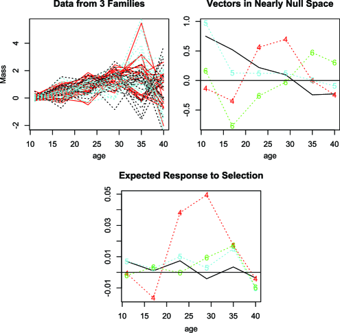
Figure 7: Results from the first simulated data set. The upper left plot shows data from three of the 100 families. The upper right plot shows vectors in the estimated nearly null space (the simplest vector in black and three PCs—PC4, PC5 and PC6). The lower left plot shows the expected responses to selection when the selection gradient is equal to each of the vectors in the upper right plot.

Figures 8 and 9 contain the results of our simulation study. In Figure 8 the upper left plot shows the 200 simplest vectors in the estimated nearly null space. The other three plots in that figure show the eigenvectors that span the estimated nearly null space. The upper right plot contains the 200 “fourth eigenvectors,” that is, those corresponding to the fourth largest eigenvalues of the estimated genetic covariance matrices. The lower left plot contains the 200 “fifth eigenvectors” and the lower right plot contains the 200 “sixth eigenvectors.”

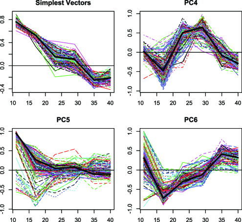
Figure 8: Simulation results from 200 data sets: the 200 simplest vectors in the estimated three-dimensional nearly null space and the eigenvectors corresponding to the three smallest eigenvalues of the estimated genetic covariance matrix along with the true eigenvectors (remaining three plots). In each plot, a true vector appears as a dark thick line. Recall that an eigenvector or simplicity vector is only defined up to a multiple of $+/{-}1$. Multipliers have been chosen so that the vectors in the above plots are similar.

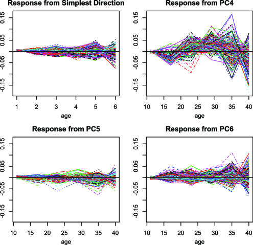
Figure 9: Simulation results from 200 data sets: expected response to selection from the simplest vector in the estimated nearly null space and the three PCs in the estimated nearly null space.

In Figure 9, the upper right plot contains the 200 expected responses to selection calculated using the 200 simplest vectors of Figure 8 as selection gradients and the “true” genetic covariance matrix. The remaining plots contain the expected responses to selection calculated using the eigenvectors shown in Figure 8 as selection gradients.

From Figures 7 to 9, we can see that the simplest vectors in the estimated nearly null spaces are always interpretable and send the same clear message. In contrast, the fourth principal components (the “dominant” component in the estimated nearly null spaces) are difficult to interpret, as we expected. The simplest vectors vary little from data set to data set and, when used as selection gradients, the simplest vectors yield expected responses to selection that are close to 0, with little variability (mean length of the response vectors is 0.032 with standard deviation 0.001). In contrast, when the fourth eigenvector is the selection gradient, the magnitudes of the expected response vectors are larger and more variable, with mean length 0.091 and standard deviation 0.007.

7 Theory

The asymptotic consistency of our method follows directly from consistency of the estimated genetic covariance matrix. Under conditions, the REML estimate $\hat{\mathcal{G}}$ is asymptotically equivalent to the maximum likelihood estimate, which converges in probability to $\mathcal{G}$, the true genetic covariance matrix [Demidenko (2004), page 181]. In this case, the eigenvalues of $\hat{\mathcal{G}}$ converge to those of $\mathcal{G}$, since eigenvalues are defined as solutions of the characteristic polynomial, and the coefficients of the characteristic polynomial of $\hat{\mathcal{G}}$ converge to those of $\mathcal{G}$. Thus, for many common methods of estimating the dimension $J$ of the model space, the dimension of the estimated model space converges to $J$, with, possibly, the requirement that $\lambda_{J}>\lambda_{J+1}$. For instance, the convergence of estimated eigenvalues implies that the proportion of variance explained by the first $J$ eigenvectors of $\hat{\mathcal{G}}$ will converge to the proportion of variance explained by the first $J$ eigenvectors of $\mathcal{G}$.

Showing convergence of estimated eigenspaces requires more care due to the complication of defining distances between subspaces and due to the possibility of multiplicity of the roots of the characteristic polynomial and the resulting nonuniqueness of eigenvectors. See Gaydos (2008), who shows that, under conditions, the nearly null space of the usual sample covariance matrix converges to that of the true covariance matrix. To define convergence, Gaydos defines the squared distance between two subspaces as the sum of the squared sines of the canonical angles between the two subspaces. See Stewart and Sun (1990) for a discussion of canonical angles.

8 Discussion

We have proposed simplicity measures and developed accompanying graphical tools to explore and visualize directions of low variability in vector-valued traits. The techniques allow us to more directly study the space spanned by the lowest variance PCs. When examined individually, these PCs typically have little structure. Considering them jointly as a subspace allows us to find the simplest structure within that subspace. Our graphical tools allow us to consider subspaces of different dimensions, easily seeing the simplicity and variance explained by the subspace and individual vectors.

Here, we have studied the nearly null space by defining a simplicity basis with the simplicity of a vector $v$ of the form $v^{\prime}\Lambda v$, and we have analyzed data with the simplicity of $v$ defined in terms of first divided differences of the components of $v$. Instead of using such a smoothing-based simplicity measure, one could consider a sparseness measure, deeming a vector to be simple if it has many zero components. In a modification of principal components, Chipman and Gu (2005) define sparseness of a vector in terms of the number of its nonzero components. Another sparseness measure, used in the varimax method of factor rotation in factor analysis [Johnson and Wichern (2008)], defines a quadratic measure of sparseness of the vector $v$, namely, $\sum({\mathrm{v}}_{i}-\bar{{\mathrm{v}}})^{2}$, with large values indicating greater simplicity. An $L_{1}$ measure of sparseness, namely, $\sum|{\mathrm{v}}_{i}|$, is used in the Lasso technique for regression [Tibshirani (1996)], with small values indicating greater simplicity.

Our methodology can, in principle, be extended to function-valued traits. Genetic constraints can be defined for function-valued traits via the work of Kirkpatrick and Heckman (1989), Gomulkiewicz and Beder (1996) and Beder and Gomulkiewicz (1998), who showed the validity of the Breeder’s equation in (1) and (2) when the phenotype is a function. The advantages of functional data analysis techniques over multivariate techniques are well known in the statistical literature. For instance, functional data analysis does not require that individuals be measured at the same time points or even at the same number of times. Furthermore, functional data analysis uses the smoothness underlying the data to avoid high-dimensional analysis problems caused by a large number of observations per individual. The advantages of functional data analysis are only just catching hold in the biological literature. See, for instance, Gomulkiewicz and Kingsolver (2006) and Griswold, Gomulkiewicz and Heckman (2008).

Defining a simplicity basis for the nearly null space is especially useful in the analysis of functional data. To see this, suppose that the genetic component $g$ is a continuous time random process. Then, under conditions, we can write $g$ in terms of its Karhunen–Loéve expansion: $g(t)=\sum_{1}^{\infty}\alpha_{j}\phi_{j}(t)$, where the $\phi_{j}$’s are orthonormal functions and the $\alpha_{j}$’s are independent with mean zero and variances $\lambda_{1}\geq\lambda_{2}\geq\cdots\,$. See, for instance, Loève (1978) or Adler and Taylor (2007). If our model for $g$ allows a countably infinite number of these variances to be positive, then the true model space for $g$ is infinite dimensional. However, since any particular data set is finite dimensional, estimates of $g$ always lie in a finite-dimensional space. Hence, the estimated model space is finite dimensional and its orthogonal complement is infinite dimensional. A natural way to study this infinite-dimensional subspace is by finding its simplest directions and seeing if these directions have any interpretable structure.

Studying the structure of low variance subspaces can provide biologists with insights into the existence of genetic constraints. But the notion of a simplicity basis and the associated visualization tools may be useful in other contexts, in particular, in providing modeling tools in the analysis of smooth high-dimensional data.

Supplement A Supplementary plots
[doi]10.1214/12-AOAS603SUPPA .pdf aoas603_suppa.pdf As previously noted, supplementary material [Gaydos et al. (2013a)] contains a complete set of plots from our data analyses, as in Figures 3 through 6.

Supplement B Nearly null space example
[doi]10.1214/12-AOAS603SUPPB .pdf aoas603_suppb.pdf An additional supplementary file [Gaydos et al. (2013b)] contains a simple example that shows the benefits of the proposed methodology.

References

- Adler and Taylor (2007) {bbook}[mr] \bauthor\bsnmAdler, \bfnmRobert J.\binitsR. J. and \bauthor\bsnmTaylor, \bfnmJonathan E.\binitsJ. E. (\byear2007). \btitleRandom Fields and Geometry. \bpublisherSpringer, \blocationNew York. \bidmr=2319516 \bptokimsref \endbibitem
- Amemiya, Anderson and Lewis (1990) {barticle}[mr] \bauthor\bsnmAmemiya, \bfnmYasuo\binitsY., \bauthor\bsnmAnderson, \bfnmT. W.\binitsT. W. and \bauthor\bsnmLewis, \bfnmPeter A. W.\binitsP. A. W. (\byear1990). \btitlePercentage points for a test of rank in multivariate components of variance. \bjournalBiometrika \bvolume77 \bpages637–641. \biddoi=10.1093/biomet/77.3.637, issn=0006-3444, mr=1087855 \bptokimsref \endbibitem
- Anderson and Amemiya (1991) {barticle}[mr] \bauthor\bsnmAnderson, \bfnmT. W.\binitsT. W. and \bauthor\bsnmAmemiya, \bfnmYasuo\binitsY. (\byear1991). \btitleTesting dimensionality in the multivariate analysis of variance. \bjournalStatist. Probab. Lett. \bvolume12 \bpages445–463. \biddoi=10.1016/0167-7152(91)90002-9, issn=0167-7152, mr=1143744 \bptokimsref \endbibitem
- Beder and Gomulkiewicz (1998) {barticle}[mr] \bauthor\bsnmBeder, \bfnmJay H.\binitsJ. H. and \bauthor\bsnmGomulkiewicz, \bfnmRichard\binitsR. (\byear1998). \btitleComputing the selection gradient and evolutionary response of an infinite-dimensional trait. \bjournalJ. Math. Biol. \bvolume36 \bpages299–319. \biddoi=10.1007/s002850050102, issn=0303-6812, mr=1608605 \bptnotecheck year\bptokimsref \endbibitem
- Chipman and Gu (2005) {barticle}[mr] \bauthor\bsnmChipman, \bfnmHugh A.\binitsH. A. and \bauthor\bsnmGu, \bfnmHong\binitsH. (\byear2005). \btitleInterpretable dimension reduction. \bjournalJ. Appl. Stat. \bvolume32 \bpages969–987. \biddoi=10.1080/02664760500168648, issn=0266-4763, mr=2221888 \bptokimsref \endbibitem
- Demidenko (2004) {bbook}[mr] \bauthor\bsnmDemidenko, \bfnmEugene\binitsE. (\byear2004). \btitleMixed Models: Theory and Applications. \bpublisherWiley, \blocationHoboken, NJ. \biddoi=10.1002/0471728438, mr=2077875 \bptokimsref \endbibitem
- Eilers and Marx (1996) {barticle}[mr] \bauthor\bsnmEilers, \bfnmPaul H. C.\binitsP. H. C. and \bauthor\bsnmMarx, \bfnmBrian D.\binitsB. D. (\byear1996). \btitleFlexible smoothing with -splines and penalties. \bjournalStatist. Sci. \bvolume11 \bpages89–121. \biddoi=10.1214/ss/1038425655, issn=0883-4237, mr=1435485 \bptnotecheck related\bptokimsref \endbibitem
- Gaydos (2008) {bmisc}[author] \bauthor\bsnmGaydos, \bfnmTravis\binitsT. (\byear2008). \bhowpublishedData representation/basis selection to understand variation of function valued traits. Ph.D. thesis, Univ. North Carolina. \bptokimsref \endbibitem
- Gaydos et al. (2013a) {bmisc}[author] \bauthor\bsnmGaydos, \bfnmT.\binitsT., \bauthor\bsnmHeckman, \bfnmN.\binitsN., \bauthor\bsnmKirkpatrick, \bfnmM.\binitsM., \bauthor\bsnmStinchcombe, \bfnmJ. R.\binitsJ. R., \bauthor\bsnmSchmitt, \bfnmJ.\binitsJ., \bauthor\bsnmKingsolver, \bfnmJ.\binitsJ. and \bauthor\bsnmMarron, \bfnmJ. S.\binitsJ. S. (\byear2013a). \bhowpublishedSupplement to “Visualizing genetic constraints.” DOI:\doiurl10.1214/12-AOAS603SUPPA. \bptokimsref \endbibitem
- Gaydos et al. (2013b) {bmisc}[author] \bauthor\bsnmGaydos, \bfnmT.\binitsT., \bauthor\bsnmHeckman, \bfnmN.\binitsN., \bauthor\bsnmKirkpatrick, \bfnmM.\binitsM., \bauthor\bsnmStinchcombe, \bfnmJ. R.\binitsJ. R., \bauthor\bsnmSchmitt, \bfnmJ.\binitsJ., \bauthor\bsnmKingsolver, \bfnmJ.\binitsJ. and \bauthor\bsnmMarron, \bfnmJ. S.\binitsJ. S. (\byear2013b). \bhowpublishedSupplement to “Visualizing genetic constraints.” DOI:\doiurl10.1214/12-AOAS603SUPPB. \bptokimsref \endbibitem
- Gomulkiewicz and Beder (1996) {barticle}[mr] \bauthor\bsnmGomulkiewicz, \bfnmRichard\binitsR. and \bauthor\bsnmBeder, \bfnmJay H.\binitsJ. H. (\byear1996). \btitleThe selection gradient of an infinite-dimensional trait. \bjournalSIAM J. Appl. Math. \bvolume56 \bpages509–523. \biddoi=10.1137/S0036139993255765, issn=0036-1399, mr=1381657 \bptokimsref \endbibitem
- Gomulkiewicz and Houle (2009) {barticle}[author] \bauthor\bsnmGomulkiewicz, \bfnmR.\binitsR. and \bauthor\bsnmHoule, \bfnmD.\binitsD. (\byear2009). \btitleDemographic and genetic constraints on evolution. \bjournalAmerican Naturalist \bvolume174 \bpages218–229. \bptokimsref \endbibitem
- Gomulkiewicz and Kingsolver (2006) {barticle}[author] \bauthor\bsnmGomulkiewicz, \bfnmR.\binitsR. and \bauthor\bsnmKingsolver, \bfnmJ. G.\binitsJ. G. (\byear2006). \btitleA fable of four functions: Function-valued approaches in evolutionary biology. \bjournalJournal of Evolutionary Biology \bvolume20 \bpages20–21. \bptokimsref \endbibitem
- Green and Silverman (1994) {bbook}[mr] \bauthor\bsnmGreen, \bfnmP. J.\binitsP. J. and \bauthor\bsnmSilverman, \bfnmB. W.\binitsB. W. (\byear1994). \btitleNonparametric Regression and Generalized Linear Models: A Roughness Penalty Approach. \bseriesMonographs on Statistics and Applied Probability \bvolume58. \bpublisherChapman & Hall, \blocationLondon. \bidmr=1270012 \bptokimsref \endbibitem
- Griswold, Gomulkiewicz and Heckman (2008) {barticle}[pbm] \bauthor\bsnmGriswold, \bfnmCortland K.\binitsC. K., \bauthor\bsnmGomulkiewicz, \bfnmRichard\binitsR. and \bauthor\bsnmHeckman, \bfnmNancy\binitsN. (\byear2008). \btitleHypothesis testing in comparative and experimental studies of function-valued traits. \bjournalEvolution \bvolume62 \bpages1229–1242. \biddoi=10.1111/j.1558-5646.2008.00340.x, issn=0014-3820, pii=EVO340, pmid=18266991 \bptokimsref \endbibitem
- Heckman (2003) {bincollection}[mr] \bauthor\bsnmHeckman, \bfnmNancy E.\binitsN. E. (\byear2003). \btitleFunctional data analysis in evolutionary biology. In \bbooktitleRecent Advances and Trends in Nonparametric Statistics (\beditor\bfnmM. G.\binitsM. G. \bsnmAkritas and \beditor\bfnmD. N.\binitsD. N. \bsnmPolitis, eds.) \bpages49–60. \bpublisherElsevier, \blocationAmsterdam. \biddoi=10.1016/B978-044451378-6/50004-1, mr=2498232 \bptokimsref \endbibitem
- Hine and Blows (2006) {barticle}[pbm] \bauthor\bsnmHine, \bfnmEmma\binitsE. and \bauthor\bsnmBlows, \bfnmMark W.\binitsM. W. (\byear2006). \btitleDetermining the effective dimensionality of the genetic variance–covariance matrix. \bjournalGenetics \bvolume173 \bpages1135–1144. \biddoi=10.1534/genetics.105.054627, issn=0016-6731, pii=genetics.105.054627, pmcid=1526539, pmid=16547106 \bptokimsref \endbibitem
- Izem and Kingsolver (2005) {barticle}[pbm] \bauthor\bsnmIzem, \bfnmRima\binitsR. and \bauthor\bsnmKingsolver, \bfnmJoel G.\binitsJ. G. (\byear2005). \btitleVariation in continuous reaction norms: Quantifying directions of biological interest. \bjournalAm. Nat. \bvolume166 \bpages277–289. \biddoi=10.1086/431314, issn=1537-5323, pii=AN40690, pmid=16032579 \bptokimsref \endbibitem
- Johnson and Wichern (2008) {bbook}[author] \bauthor\bsnmJohnson, \bfnmRichard A.\binitsR. A. and \bauthor\bsnmWichern, \bfnmDean W.\binitsD. W. (\byear2008). \btitleApplied Multivariate Statistical Analysis, \bedition6th ed. \bpublisherPearson Education, \blocationUpper Saddle River. \bptokimsref \endbibitem
- Kingsolver, Gomulkiewicz and Carter (2001) {barticle}[author] \bauthor\bsnmKingsolver, \bfnmJoel G.\binitsJ. G., \bauthor\bsnmGomulkiewicz, \bfnmRichard\binitsR. and \bauthor\bsnmCarter, \bfnmPatrick A.\binitsP. A. (\byear2001). \btitleVariation, selection and evolution of function valued traits. \bjournalGenetica \bvolume112–113 \bpages87–104. \bptokimsref \endbibitem