Hermite subdivision schemes, exponential polynomial generation, and annihilators

Abstract

We consider the question when the so–called spectral condition for Hermite subdivision schemes extends to spaces generated by polynomials and exponential functions. The main tool are convolution operators that annihilate the space in question which apparently is a general concept in the study of various types of subdivision operators. Based on these annihilators, we characterize the spectral condition in terms of factorization of the subdivision operator.

Keywords subdivision schemes; Hermite schemes; factorization; annihilators

MSC 65D15; 41A05; 42C15

1 Introduction

Subdivision schemes are efficient iterative procedures based on the repeated application of subdivision operators which might differ at different levels of iteration. Whenever convergent, they generate functions that hopefully resemble the data used to start the iterative procedure.

Subdivision operators act on bi-infinite sequences ${\boldsymbol{c}}:\mathbb{Z}\to\mathbb{R}$ by means of a finitely supported mask ${\boldsymbol{a}}:\mathbb{Z}\to\mathbb{R}$ in the convolution–like form

$${\cal S}_{\boldsymbol{a}}{\boldsymbol{c}}=\sum_{\beta\in\mathbb{Z}}a(\cdot-2\beta)\,c(\beta).$$

This type of operators has been generalized in various ways, considering multivariate operators, operators with dilation factors other than $2$ or subdivision operators acting on vector or matrix data by means of matrix valued masks. There is such a vast amount of literature meanwhile that we do not even attempt to give references here.

It has been observed from very early on that preservation of polynomial data is an important property of subdivision operators. For example, the preservation of constants, ${\cal S}_{\boldsymbol{a}}1=1$, is necessary for the convergence of the subdivision schemes which iterate the same operator ${\cal S}_{\boldsymbol{a}}$. More generally, the preservation of polynomial spaces, ${\cal S}_{\boldsymbol{a}}\Pi_{n}=\Pi_{n}$, plays an important role in the investigation of the differentiability of the limit function of subdivision schemes. In addition, there has been interest in also preserving functions other than polynomials, see for example [8], and it is natural that such functions must be exponential, i.e., of the form $e^{\lambda\cdot}$, cf. [9].

In this paper we will consider preservation of such exponentials by Hermite subdivision operators which act on vector data but with the particular understanding that these vectors represent function values and consecutive derivatives up to a certain order. We will study the preservation capability of such operators by means of a cancellation operator, a concept that applies to subdivision schemes in quite some generality. This is why, before we get to the main technical content of the paper, we want to illustrate the idea and the concept through a few examples.

The simplest example deals with the preservation of constants, ${\cal S}_{\boldsymbol{a}}1=1$. Note that constant sequences are exactly the kernel of the difference operator $\Delta$, defined as $\Delta{\boldsymbol{c}}=c(\cdot+1)-c$; in other words: the difference operator is the simplest cancellation operator or annihilator of the constant functions. Now, whenever ${\cal S}_{\boldsymbol{a}}$ preserves constants, then ${\cal S}_{\boldsymbol{c}}=\Delta{\cal S}_{\boldsymbol{a}}$ is a subdivision operator that annihilates the constants. As it can easily be shown, any such operator can be written as ${\cal S}_{\boldsymbol{c}}={\cal S}_{\boldsymbol{b}}\Delta$ for some other finitely supported mask ${\boldsymbol{b}}$, hence we get the factorization $\Delta{\cal S}_{\boldsymbol{a}}={\cal S}_{\boldsymbol{b}}\Delta$. Switching to the calculus of symbols which associates to a finitely supported sequence ${\boldsymbol{a}}$ the Laurent polynomial

$$a^{*}(z):=\sum_{\alpha\in\mathbb{Z}}a(\alpha)\,z^{\alpha},$$

the factorization is equivalent to $(z^{-1}-1)a^{*}(z)=b^{*}(z)(z^{-2}-1)$ or, equivalently, to the famous “zero at $\pi$” condition $a^{*}(z)=\left(z^{-1}+1\right)\,b^{*}(z)$.

For a slightly more sophisticated example, suppose that now the subdivision operator provides preservation of the subspace

$$V_{d,\Lambda}=\mbox{span}\,\left\{1,x,\dots,x^{p},e^{\lambda_{1}x},e^{-\lambda_{1}x},\dots,e^{\lambda_{r}x},e^{-\lambda_{r}x}\right\},\qquad d=p+2r+1,$$ (1)

in the sense that ${\cal S}_{\boldsymbol{a}}V^{0}_{d,\Lambda}\subseteq V^{1}_{d,\Lambda}$ where $V^{j}_{d,\Lambda}:=\left\{v(2^{-j}\cdot)\;:\;v\in V_{d,\Lambda}\right\}$, see, for example, [2, 9]. Again we approach this problem in terms of cancellation, therefore determining an operator ${\cal H}_{d,\Lambda}$ such that ${\cal H}_{d,\Lambda}V^{0}_{d,\Lambda}=\{0\}$. Assuming that ${\cal H}_{d,\Lambda}$ is a convolution operator (or LTI filter in the language of signal processing, cf. [6]) with impulse response ${\boldsymbol{h}}$, it is easily seen and well–known that cancellation of the polynomials of degree at most $p$ implies that $\left(h^{*}\right)^{(k)}(1)=0$, $k=0,\dots,p$, hence cancellation of the polynomial part of $V_{d,\Lambda}$ implies that $h^{*}(z)=\left(z^{-1}-1\right)^{p+1}\,b_{1}^{*}(z)$. Cancellation of an exponential sequence $e^{\lambda\cdot}$, on the other hand, leads to

$$0 = \sum_{j\in\mathbb{Z}}h(\cdot-j)e^{\lambda j}=\sum_{j\in\mathbb{Z}}h(j)e^{\lambda(\cdot-j)}=e^{\lambda\cdot}h^{*}(e^{-\lambda}),$$

hence, the annihilation of the space implies that

$$h^{*}(z)=b_{2}^{*}(z)\,\prod_{j=1}^{r}\left(z^{-1}-e^{\lambda_{j}}\right)\left(z^{-1}-e^{-\lambda_{j}}\right).$$

Summarizing, the simplest cancellation operator for $V_{d,\Lambda}$ takes the form

$$h_{d,\Lambda}^{*}(z)=(z^{-1}-1)^{p+1}\,\prod_{j=1}^{r}\left(z^{-1}-e^{\lambda_{j}}\right)\left(z^{-1}-e^{-\lambda_{j}}\right),$$

and the associated factorization by means of cancellation operators

$${\cal H}_{d,2^{-1}\Lambda}{\cal S}_{\boldsymbol{a}}={\cal S}_{\boldsymbol{b}}{\cal H}_{d,\Lambda}$$ (2)

is easily verified to be equivalent to the symbol factorization

$$a^{*}(z)=b^{*}(z)\,(z^{-1}+1)^{p+1}\,\prod_{j=1}^{r}\left(z^{-1}+e^{\lambda_{j}/2}\right)\left(z^{-1}+e^{-\lambda_{j}/2}\right),$$ (3)

given in [9]. Note that in (2) one really has to consider different spaces, hence a preservation property of the form ${\cal S}_{\boldsymbol{a}}V^{0}_{d,\Lambda}\subseteq V^{1}_{d,\Lambda}$ because the result of the subdivision operator corresponds to a sequence on the grid $\mathbb{Z}/2$.

The last example considers Hermite subdivision schemes which we will investigate in more detail in the rest of this paper. In Hermite subdivision, the data are vector valued sequences ${\boldsymbol{v}}\in\ell^{d+1}(\mathbb{Z})$ with the intuition that the $k$–th component of such a sequence represents a $k$–th derivative. Then, as considered for example in [3, 5, 7], one defines, for $f\in C^{d}(\mathbb{R})$, a sequence

$${\boldsymbol{v}}_{f}\;:\;\alpha\mapsto\left[f^{(j)}(\alpha)\;:\;j=0,\dots,d\right],\qquad\alpha\in\mathbb{Z},$$

and asks when a subdivision operator ${\cal S}_{\boldsymbol{C}}$ with matrix valued masks ${\boldsymbol{C}}\in\ell_{00}^{d\times d}(\mathbb{Z})$ annihilates all ${\boldsymbol{v}}_{p}$ for $p\in\Pi_{d}$ which, by the aforementioned machinery, can again be used to describe the spectral condition, a “polynomial preservation” rule introduced by Dubuc and Merrien in [5]. Note that it is no mistake or accident that the letter $d$ appears for the maximal order of derivatives and the maximal degree of polynomial cancellation – the space dimension and the order of derivatives are closely tied. It was then shown in [7] that whenever ${\cal S}_{\boldsymbol{C}}{\boldsymbol{v}}_{p}=0$ for all $p\in\Pi_{d}$, then there exist a finitely supported ${\boldsymbol{B}}\in\ell_{00}^{(d+1)\times(d+1)}(\mathbb{Z})$ such that

$$C^{*}(z)=B^{*}(z)\,T_{d}^{*}(z^{2}),\qquad T_{d}^{*}(z):=\left[\begin{array}[]{cccc}z^{-1}-1&\frac{1}{2}&\dots&-\frac{1}{(d+1)!}\\ &z^{-1}-1&\dots&-\frac{1}{d!}\\ &&\ddots&\vdots\\ &&&z^{-1}-1\end{array}\right].$$

Since the operator ${\cal T}$ acts for $f\in C^{d+1}$, $k=0,\cdots,d$, as

$$\left({\cal T}v_{f}\right)_{k}(\alpha)=f^{(k)}(\alpha+1)-\sum_{j=0}^{d-k}\frac{f^{(k+j)}(\alpha)}{j!}=f^{(d+1)}(\xi_{k}),\qquad\xi_{k}\in(\alpha,\alpha+1),$$ (4)

hence measures the difference between a function and its Taylor polynomial approximation at the neighboring point, it is called the (complete) Taylor operator of order $d$. That ${\cal T}$ annihilates all ${\boldsymbol{v}}_{p}$, $p\in\Pi_{d}$, is immediate from (4).

It should have become clear by now that there is an obvious common structure behind all these examples. Preservation of a subspace that can be written as the kernel of a convolution operator is related to a commuting property provided that the convolution operator factorize-s or “divides” any annihilator of the subspace. This can be seen as a minimality property with respect to the partial ordering given by divisibility and justifies the following terminology where we identify any function $f\in V$ with the sequence ${\boldsymbol{f}}=\left(f(\alpha)\;:\;\alpha\in\mathbb{Z}\right)$.

Definition 1

A linear operator ${\cal H}:\ell^{m}(\mathbb{Z})\to\ell^{m}(\mathbb{Z})$ is called a convolution operator for a space $V$ if there exists a matrix sequence ${\boldsymbol{H}}\in\ell^{m\times m}(\mathbb{Z})$, called the impulse response of ${\cal H}$, such that

$${\cal H}{\boldsymbol{f}}={\boldsymbol{H}}*{\boldsymbol{f}}=\sum_{\beta\in\mathbb{Z}}H(\cdot-\alpha)f(\alpha),\qquad{\boldsymbol{f}}\in V.$$

Definition 2

A convolution operator ${\cal H}:\ell^{m}(\mathbb{Z})\to\ell^{m}(\mathbb{Z})$ is called a minimal annihilator for a space $V$ with respect to

1. subdivision, if for any ${\boldsymbol{C}}\in\ell^{m\times m}_{00}(\mathbb{Z})$ such that ${\cal S}_{\boldsymbol{C}}V=0$ there exists ${\boldsymbol{B}}\in\ell^{m\times m}_{00}(\mathbb{Z})$ with ${\cal S}_{\boldsymbol{C}}={\cal S}_{\boldsymbol{B}}{\cal H}$.

2. convolution, if for any ${\boldsymbol{C}}\in\ell^{m\times m}_{00}(\mathbb{Z})$ such that ${\boldsymbol{C}}*V=\{0\}$ there exists ${\boldsymbol{B}}\in\ell^{m\times m}_{00}(\mathbb{Z})$ with ${\boldsymbol{C}}={\boldsymbol{B}}*{\boldsymbol{H}}$,

respectively. If ${\cal H}$ satisfies both properties it is simply called a minimal annihilator.

The goal of this paper is to use this general concept to understand preservation of exponentials and polynomials by Hermite subdivision schemes where the subdivision operators will have to vary with the iteration level; some call this nonstationary, some nonuniform operators, but the problem is too interesting to dwell on such niceties here and therefore we omit it as the name of a property that is not fulfilled anyway is simply irrelevant.

In more technical terms, we will derive the analogy of the Taylor operator for the case of preservation of exponentials and prove in Theorem 20 that it is again a minimal annihilator. We will see that even the cancellation operator depends only on the space $V_{d,\Lambda}$ and on the level. We will also see that the existence of the annihilator operator is strongly connected with the factorization of the subdivision operator satisfying specific preservation properties.

The organization of the paper is as follows. After providing the necessary notation and terminology, the main results on Hermite subdivision schemes and their reproduction capabilities will be derived in Section 3. To better explain the underlying ideas, we will first consider the case of adding a single frequency to the polynomial space and then extend the results and methods to an arbitrary number of frequencies. These descriptions will be in terms of appropriate cancellation operators. Thereafter, in Section 4 we will use these cancellation operators to derive factorization properties which will also verify that the cancellation operators are minimal. Finally, we will illustrate our results with specific examples.

2 Subdivision schemes and notation

We begin by fixing the notation and recalling some known facts about subdivision schemes. We denote by $\ell^{m}\left(\mathbb{Z}\right)$ and $\ell^{m\times m}\left(\mathbb{Z}\right)$ the linear spaces of all sequences of $m$–vectors and $m\times m$ matrices, respectively. Operators acting on that spaces are denoted by capital calligrafic letter. Sequences in $\ell^{m}\left(\mathbb{Z}\right)$ and $\ell^{m\times m}\left(\mathbb{Z}\right)$ will be denoted by boldface lower case and upper case letters, respectively. In particular, ${\boldsymbol{c}}\in\ell^{m}\left(\mathbb{Z}\right)$ is ${\boldsymbol{c}}=\left(c(\alpha)\;:\;\alpha\in\mathbb{Z}\right)$, while ${\boldsymbol{A}}\in\ell^{m\times m}\left(\mathbb{Z}\right)$ stands for ${\boldsymbol{A}}=\left(A(\alpha)\;:\,\alpha\in\mathbb{Z}\right)$, indexing $A\in\mathbb{R}^{m\times m}$ as $A=\left[a_{jk}:\,j,k=0,\dots,m-1\right]$. As usual, $\ell_{00}^{m}\left(\mathbb{Z}\right)$ and $\ell_{00}^{m\times m}\left(\mathbb{Z}\right)$ will denote the subspaces of finitely supported sequences, and $\mathbb{N}_{0}$ denotes the set $\{0,1,2,\ldots\}$.

For ${\boldsymbol{A}}\in\ell_{00}^{m\times m}\left(\mathbb{Z}\right)$ and ${\boldsymbol{c}}\in\ell_{00}^{m}\left(\mathbb{Z}\right)$ we define the associated symbols as the Laurent polynomials

$$A^{*}(z):=\sum_{\alpha\in\mathbb{Z}}A(\alpha)\,z^{\alpha},\qquad c^{*}(z):=\sum_{\alpha\in\mathbb{Z}}c(\alpha)\,z^{\alpha},\qquad z\in\mathbb{C}\setminus\{0\}.$$

For ${\boldsymbol{A}}\in\ell_{00}^{m\times r}\left(\mathbb{Z}\right)$ and ${\boldsymbol{B}}\in\ell_{00}^{r\times q}\left(\mathbb{Z}\right)$ the convolution ${\boldsymbol{C}}={\boldsymbol{A}}*{\boldsymbol{B}}$ in $\ell_{00}^{m\times q}\left(\mathbb{Z}\right)$ is defined as usually as

$$C(\alpha):=\sum_{\beta\in\mathbb{Z}}A(\beta)B(\alpha-\beta),\qquad\alpha\in\mathbb{Z}.$$

The subdivision operator ${\cal S}_{\boldsymbol{A}}:\ell^{m}(\mathbb{Z})\rightarrow\ell^{m}(\mathbb{Z})$ based on the matrix sequence or mask ${\boldsymbol{A}}\in\ell^{m\times m}_{00}(\mathbb{Z})$ is defined as

$${\cal S}_{\boldsymbol{A}}{\boldsymbol{c}}(\alpha)=\sum_{\beta\in\mathbb{Z}}A\left(\alpha-2\beta\right)c(\beta),\qquad\alpha\in\mathbb{Z},\qquad\hbox{for all}\ {\boldsymbol{c}}\in\ell^{m}\left(\mathbb{Z}\right).$$ (5)

Alternatively, using symbol calculus notation, we can also decribe the action of the subdivision operator in the form

$$\left({\cal S}_{\boldsymbol{A}}{\boldsymbol{c}}\right)^{*}(z)=A^{*}(z)\,c^{*}\left(z^{2}\right),\qquad z\in\mathbb{C}\setminus\{0\},$$ (6)

though, in strict formalism, (6) is only valid for ${\boldsymbol{c}}\in\ell_{00}^{m}(\mathbb{Z})$.

A subdivision scheme consists of the successive application of potentially different subdivision operators ${\cal S}_{{\boldsymbol{A}}^{[n]}}$, constructed from a sequence of masks $\left({\boldsymbol{A}}^{[n]}\;:\;n\in\mathbb{N}_{0}\right)$ where ${\boldsymbol{A}}^{[n]}=\left(A^{[n]}(\alpha)\;:\;\alpha\in\mathbb{Z}\right)\in\ell_{00}^{m\times m}(\mathbb{Z})$ is called the level $n$ subdivision mask and is assumed to be of finite support. Accordingly, a sequence of matrix symbols $\left((A^{[n]})^{*}(z)\;:\;n\in\mathbb{N}_{0}\right)$ characterizes such schemes.

For some initial sequence ${\boldsymbol{c}}^{[0]}\in\ell^{m}(\mathbb{Z})$ the subdivision scheme iteratively produces sequences

$${\boldsymbol{c}}^{[n+1]}:={\cal S}_{{\boldsymbol{A}}^{[n]}}{\boldsymbol{c}}^{[n]},\qquad n\in\mathbb{N}_{0},$$

whose elements can be interpreted as function values at $2^{-n-1}\mathbb{Z}$, from which one can define convergence in the usual way.

3 Hermite subdivision schemes and reproduction

As already mentioned, Hermite subdivision schemes act on vector valued data ${\boldsymbol{c}}\in\ell^{d+1}(\mathbb{Z})$, whose $k$-th component corresponds to a $k$–th derivative. We are interested in studying the exponential and polynomial preservation capabilities of such kind of schemes.

A preliminary simple observation is that for $f\in C^{d}(\mathbb{R})$ and for $g:=f(2^{-n}\cdot)$ we clearly have $\frac{d^{r}}{dx^{r}}g=2^{-nr}\frac{d^{r}f}{dx^{r}}f(2^{-n}\cdot)$, $r=0,\cdots,d$. Hence

$$\left[\frac{d^{j}}{dx^{j}}f(2^{n}\cdot):\,j=0,\dots,d\right]=D^{n}\left[f^{(j)}(2^{-n}\cdots):\,j=0,\dots,d\right],$$ (7)

where

$$D=\left[\begin{array}[]{ccccc}1&0&0&\cdots&0\\ 0&\frac{1}{2}&0&\cdots&0\\ \vdots\\ 0&0&0&\cdots&\frac{1}{2^{d}}\end{array}\right].$$

Since the sequence ${\boldsymbol{c}}^{[n]}$ is related to evaluations on the grid $2^{-n}\mathbb{Z}$, we consider Hermite subdivision schemes with the $n$-th iteration of the following type:

$$D^{n+1}{\boldsymbol{c}}^{[n+1]}=\sum_{\beta\in\mathbb{Z}}A^{[n]}(\cdot-2\beta)D^{n}c^{[n]}(\beta),$$ (8)

where in “usual” Hermite subdivision the mask is the same over all levels, i.e., ${\boldsymbol{A}}^{[n]}={\boldsymbol{A}}$, $n\in\mathbb{N}_{0}$. Setting $\widetilde{\boldsymbol{A}}^{[n]}:=D^{-n-1}{\boldsymbol{A}}^{[n]}D^{n}$, (8) fits into the framework of Section 2 with the $n$-th subdivision operator of the form

$${\boldsymbol{c}}^{[n+1]}=S_{\widetilde{A}^{[n]}}{\boldsymbol{c}}^{[n]}=\sum_{\beta\in\mathbb{Z}}\widetilde{A}^{[n]}(\cdot-2\beta)\,c^{[n]}(\beta).$$ (9)

3.1 Single exponential frequency

In the first step of our analysis of the stepwise reproduction capability of a Hermite subdivision scheme of type (8), we add only a single pair of exponentials $e^{\pm\lambda x}$ and consider the space

$$V_{d,\lambda}=\mbox{\rm span}\left\{1,x,\ldots,x^{d-2},e^{\lambda x},e^{-\lambda x}\right\},\qquad\lambda\in\mathbb{R}\cup i\mathbb{R}.$$ (10)

To keep notation simple and to better explain the underlying ideas, we will first carefully investigate this situation and then extend it in a quite straightforward fashion to the general case.

Remark 3

As can be seen in (10), the addition of an exponential frequency $\lambda$ always means the addition of the pair $e^{\pm\lambda\cdot}$ of functions. On the one hand, this is motivated by the fact that choosing $\lambda=i$ equals reproduction of the trigonometric functions $\sin x$ and $\cos x$. Moreover, our approach to construct the annihilator and the factorization actually strongly depends on the presence of this pair of frequencies. Whether or not similar results will be available for the case where only $e^{\lambda\cdot}$ but not $e^{-\lambda\cdot}$, we do not know at present.

For any function $f\in C^{d}(\mathbb{R})$ and any integer $n\in\mathbb{N}_{0}$ we consider the two vector sequences ${\widetilde{\boldsymbol{v}}}_{f,{n}}$, ${\boldsymbol{v}}_{f,{n}}\in\ell^{d+1}(\mathbb{Z})$, defined, for $\alpha\in\mathbb{Z}$, as

$$\widetilde{v}_{f,{n}}(\alpha):=\left[\begin{array}[]{c}f(2^{-n}\alpha)\\ f^{\prime}(2^{-n}\alpha)\\ \vdots\\ f^{(d)}(2^{-n}\alpha)\end{array}\right],\qquad v_{f,{n}}(\alpha):=D^{n}\widetilde{v}_{f,{n}}(\alpha)=\left[\begin{array}[]{c}f(2^{-n}\alpha)\\ 2^{-n}f^{\prime}(2^{-n}\alpha)\\ \vdots\\ 2^{-nd}f^{(d)}(2^{-n}\alpha)\end{array}\right].$$

We simply write ${\boldsymbol{v}}_{f}=\widetilde{\boldsymbol{v}}_{f}$ when $n=0$.

Definition 4

A mask ${\boldsymbol{A}}^{[n]}\in\ell_{00}^{(d+1)\times(d+1)}(\mathbb{Z})$ or its associated subdivision operator ${\cal S}_{{{\boldsymbol{A}}}^{[n]}}$ satisfies the $V_{d,\lambda}$-spectral condition if

$${\cal S}_{{{\boldsymbol{A}}}^{[n]}}{\boldsymbol{v}}_{f,n}={\boldsymbol{v}}_{f,{n+1}},\qquad f\in V_{d,\lambda}.$$

Equivalently, the mask $\widetilde{\boldsymbol{A}}^{[n]}=D^{-(n+1)}{\boldsymbol{A}}^{[n]}D^{n}$ satisfies the $V_{d,\lambda}$-spectral condition if

$${\cal S}_{\widetilde{\boldsymbol{A}}^{[n]}}{\widetilde{\boldsymbol{v}}}_{f,n}={\widetilde{\boldsymbol{v}}}_{f,{n+1}},\qquad f\in V_{d,\lambda}.$$

Remark 5

It is important to observe that Definition 4 is fully consistent with [7, Definition 1] though formulated in a slightly different way taking into account the stronger form of level dependency needed for the reproduction of exponentials.

Since we plan to extend difference operators and Taylor operators, we next recall their formal definitions.

Definition 6

The Taylor operator ${\cal T}_{d}$ of order $d$, acting on $\ell^{d+1}(\mathbb{Z})$ is defined as

$${\cal T}_{d}:=\left[\begin{array}[]{ccccc}\Delta&-1&\cdots&-\frac{1}{(d-1)!}&-\frac{1}{d!}\\ &\Delta&\ddots&\vdots&\vdots\\ &&\ddots&-1&\vdots\\ &&&\Delta&-1\\ &&&&\Delta\end{array}\right],$$ (11)

where $\Delta$ is the forward difference operator.

The symbol of the Taylor operator then takes the form

$$T_{d}^{*}(z):=\left[\begin{array}[]{ccccc}(z^{-1}-1)&-1&\cdots&-\frac{1}{(d-1)!}&-\frac{1}{d!}\\ &(z^{-1}-1)&\ddots&\vdots&\vdots\\ &&\ddots&-1&\vdots\\ &&&(z^{-1}-1)&-1\\ &&&&(z^{-1}-1)\end{array}\right].$$ (12)

Definition 7

A level-$n$ cancellation operator ${\cal H}^{[n]}:\ell^{d+1}(\mathbb{Z})\to\ell^{d+1}(\mathbb{Z})$ for a linear function space $V\subset C^{d}(\mathbb{R})$ is a convolution operator such that

$${\cal H}^{[n]}{\boldsymbol{v}}_{f,n}=\sum_{\alpha\in\mathbb{Z}}H^{[n]}(\cdot-\alpha)v_{f,n}(\alpha)=0,\qquad f\in V.$$ (13)

By ${\cal H}^{[n]}_{d,\lambda}$ we denote a level-$n$ cancellation operator for the function space spanned by $V_{d,\lambda}$.

Lemma 8

An operator ${\cal H}^{[n]}_{d,\lambda}$ is a level-$n$ cancellation operator for the space $V_{d,\lambda}$ if it satisfies

$$\left(H^{[n]}_{d,\lambda}\right)^{*}(z)=\left[\begin{array}[]{cc}T^{*}_{d-2}(z)&*\\ 0&*\end{array}\right]$$ (14)

and

$$\left(H^{[n]}_{d,\lambda}\right)^{*}\left(e^{\mp 2^{-n}\lambda}\right)D^{n}\left[\begin{array}[]{c}1\\ \pm\lambda\\ \vdots\\ (\pm\lambda)^{d}\end{array}\right]=0.$$ (15)

Proof:  To annihilate polynomials of degree $d-2$, condition (13) has to be satisfied for the vector sequences

$${\boldsymbol{v}}_{(\cdot)^{j},n}=D^{n}\left[(2^{-n}\cdot)^{j},j(2^{-n}\cdot)^{j-1},\dots,j!,\underbrace{0,\,0,\cdots,\,0}_{d-j}\right]^{T},\qquad j=0,\ldots,d-2,$$

and since these sequences are exactly annihilated by the complete Taylor operator as shown in [7], any decomposition of the form (14) annihilates polynomials of degree at most $d-2$.

To describe cancellation of exponentials, we first observe that

$${\boldsymbol{v}}_{e^{\pm\lambda\cdot},n}=e^{\pm\lambda 2^{-n}\cdot}D^{n}\left[\begin{array}[]{c}1\\ \pm\lambda\\ \vdots\\ (\pm\lambda)^{d}\end{array}\right],$$

so that the condition becomes

$$0 = \sum_{\alpha\in\mathbb{Z}}H_{d,\lambda}^{[n]}(\cdot-\alpha)\,e^{\pm 2^{-n}\lambda\alpha}D^{n}\left[\begin{array}[]{c}1\\ \pm\lambda\\ \vdots\\ (\pm\lambda)^{d}\end{array}\right]$$

$$= \sum_{\alpha\in\mathbb{Z}}H_{d,\lambda}^{[n]}(\alpha)\,e^{\pm 2^{-n}\lambda(\cdot-\alpha)}D^{n}\left[\begin{array}[]{c}1\\ \pm\lambda\\ \vdots\\ (\pm\lambda)^{d}\end{array}\right]$$

$$= e^{\pm 2^{-n}\lambda\cdot}\left(H_{d,\lambda}^{[n]}\right)^{*}(e^{\mp 2^{-n}\lambda})\,D^{n}\left[\begin{array}[]{c}1\\ \pm\lambda\\ \vdots\\ (\pm\lambda)^{d}\end{array}\right]$$

which yields (15). $\Box$

Remark 9

If we are able to find an operator ${\cal H}_{d,\lambda}$ that satisfies (14) and

$$H_{d,\lambda}^{*}\left(e^{\mp\lambda}\right)\left[\begin{array}[]{c}1\\ \pm\lambda\\ \vdots\\ (\pm\lambda)^{d}\end{array}\right]=0,$$ (19)

then we automatically obtain level-$n$ cancellation operators ${\cal H}^{[n]}_{d,\lambda}$ for any $n\in\mathbb{N}_{0}$ by setting

$${\cal H}^{[n]}_{d,\lambda}={\cal H}_{d,2^{-n}\lambda}.$$

In fact, this follows from the simple observation that the identity

$$H_{d,2^{-n}\lambda}^{*}\left(e^{\mp 2^{-n}\lambda}\right)D^{n}\left[\begin{array}[]{c}1\\ \pm\lambda\\ \vdots\\ (\pm\lambda)^{d}\end{array}\right]=H_{d,2^{-n}\lambda}^{*}\left(e^{\mp 2^{-n}\lambda}\right)\left[\begin{array}[]{c}1\\ \pm\frac{\lambda}{2^{n}}\\ \vdots\\ (\pm\frac{\lambda}{2^{n}})^{d}\end{array}\right]=0,$$

is equivalent to (19), as can be verified by just replacing $\lambda$ with $2^{-n}\lambda$.

In view of Remark 9 we see that to generate a level-$n$ cancellation operator we just need to construct a level-$0$ cancellation operator. Therefore we continue with the analysis of ${\cal H}^{[0]}_{d,\lambda}$ which will be simply denoted by ${\cal H}_{d,\lambda}$.

The next step is now to construct a cancellation operator which will eventually even turn out to be a minimal one. Based on Lemma 8, the structure of the cancellation operator ${\cal H}_{d,\lambda}$ for the space $V_{d,\lambda}$ can now be derived. Indeed, we write its symbol in the general form

$$H_{d,\lambda}^{*}(z)=\left[\begin{array}[]{cc}T_{d-2}^{*}(z)&Q^{*}(z)\\ 0&R^{*}(z)\end{array}\right],\quad Q^{*}(z)\in\mathbb{R}^{(d-2)\times 2},\,R^{*}(z)\in\mathbb{R}^{2\times 2}$$ (20)

and determine the remaining part of $H_{d,\lambda}^{*}(z)$, namely the Laurent polynomial matrices $Q^{*}(z)$ and $R^{*}(z)$. To this aim, we begin to explicitly compute the first line $(H^{*}_{d,\lambda})_{0,:}(z)$, where the “$:$” is to be understood in the sense of Matlab notation.

Lemma 10

The condition

$$(H^{*}_{d,\lambda})_{0,:}\left(e^{\mp\lambda}\right)\left[\begin{array}[]{c}1\\ \pm\lambda\\ \vdots\\ (\pm\lambda)^{d}\end{array}\right]=0\,,$$ (21)

can be fulfilled by setting

$$(H_{d,\lambda})_{0,d-1}=h_{0,d-1}=\frac{\lambda^{1-d}}{2}\left\{\begin{array}[]{lcl}e^{-\lambda}-e^{\lambda}+2\displaystyle\sum_{2j+1\leq d-2}\frac{\lambda^{2j+1}}{(2j+1)!},&&d\in 2\mathbb{Z},\\ -\left(e^{-\lambda}+e^{\lambda}-2\displaystyle\sum_{2j\leq d-2}\frac{\lambda^{2j}}{(2j)!}\right),&&d\in 2\mathbb{Z}+1,\end{array}\right.$$ (22)

and

$$(H_{d,\lambda})_{0,d}=h_{0,d}=\frac{\lambda^{-d}}{2}\left\{\begin{array}[]{lcl}-\left(e^{-\lambda}+e^{\lambda}+2\displaystyle\sum_{2j\leq d-2}\frac{\lambda^{2j}}{(2j)!}\right),&&d\in 2\mathbb{Z},\\ e^{-\lambda}-e^{\lambda}+2\displaystyle\sum_{2j+1\leq d-2}\frac{\lambda^{2j+1}}{(2j+1)!},&&d\in 2\mathbb{Z}+1,\end{array}\right.$$ (23)

Proof:  Due to (12), the identity (21) can be written as

$$0 = e^{\pm\lambda}-1-\sum_{j=1}^{d-2}\frac{(\pm\lambda)^{k}}{k!}+(\pm\lambda)^{d-1}h_{0,d-1}+(\pm\lambda)^{d}h_{0,d}$$

$$= e^{\pm\lambda}-t_{d-2}\left[e^{\pm\lambda\cdot}\right](1)+(\pm\lambda)^{d-1}h_{0,d-1}+(\pm\lambda)^{d}h_{0,d},$$

where

$$t_{k}[f]=\sum_{j=0}^{k}\frac{f^{(j)}(0)}{j!}(\cdot)^{j}\,,$$

denotes the Taylor polynomial of $f$ of order $k$ expanded at $0$. Adding and subtracting the above conditions we get

$$0 = \left(e^{\lambda}\pm e^{-\lambda}\right)-t_{d-2}\left[e^{\lambda\cdot}\pm e^{-\lambda\cdot}\right](1)$$

$$\quad+\left(\lambda^{d-1}\pm(-\lambda)^{d-1}\right)h_{0,d-1}+\left(\lambda^{d}\pm(-\lambda)^{d}\right)h_{0,d}.$$

If $d$ is even, this implies that

$$h_{0,d-1} = \frac{e^{-\lambda}-e^{\lambda}-t_{d-2}\left[e^{-\lambda\cdot}-e^{\lambda\cdot}\right](1)}{2\lambda^{d-1}},$$

$$h_{0,d} = -\frac{e^{-\lambda}+e^{\lambda}-t_{d-2}\left[e^{-\lambda\cdot}+e^{\lambda\cdot}\right](1)}{2\lambda^{d}},$$

while for odd $d$ we get

$$h_{0,d-1} = -\frac{e^{-\lambda}+e^{\lambda}-t_{d-2}\left[e^{-\lambda\cdot}+e^{\lambda\cdot}\right](1)}{2\lambda^{d-1}},$$

$$h_{0,d} = \frac{e^{-\lambda}-e^{\lambda}-t_{d-2}\left[e^{-\lambda\cdot}-e^{\lambda\cdot}\right](1)}{2\lambda^{d}}.$$

Since

$$\frac{d^{k}}{dx^{k}}\left(e^{\lambda x}\pm e^{-\lambda x}\right)=\lambda^{k}\left(e^{\lambda x}\pm(-1)^{k}e^{-\lambda x}\right),$$

we have that

$$t_{d-2}\left[e^{\lambda\cdot}-e^{-\lambda\cdot}\right](1)=2\lambda+\frac{2}{3}\lambda^{3}+\cdots=2\sum_{2j+1\leq d-2}\frac{\lambda^{2j+1}}{(2j+1)!}\,,$$

and

$$t_{d-2}\left[e^{\lambda\cdot}+e^{-\lambda\cdot}\right](1)=2+\lambda^{2}+\cdots=2\sum_{2j\leq d-2}\frac{\lambda^{2j}}{(2j)!}.$$

Substituting these identities readily gives (22) and (23). $\Box$

Taking into account the structure of $H_{d,\lambda}^{*}(z)$, we can now easily give also the entries of the other lines.

Corollary 11

For $k=0,\dots,d-2$, we have that

$$h_{k,d-1} = \frac{\lambda^{1-d+k}}{2}\left\{\begin{array}[]{lcl}e^{-\lambda}-e^{\lambda}+2\displaystyle\sum_{2j+1\leq d-2-k}\frac{\lambda^{2j+1}}{(2j+1)!},&&d-k\in 2\mathbb{Z},\\ -\left(e^{-\lambda}+e^{\lambda}-2\displaystyle\sum_{2j\leq d-2-k}\frac{\lambda^{2j}}{(2j)!}\right),&&d-k\in 2\mathbb{Z}+1,\end{array}\right.$$ (26)

$$h_{k,d} = \frac{\lambda^{-d+k}}{2}\left\{\begin{array}[]{lcl}-\left(e^{-\lambda}+e^{\lambda}-2\displaystyle\sum_{2j\leq d-2-k}\frac{\lambda^{2j}}{(2j)!}\right),&&d-k\in 2\mathbb{Z},\\ e^{-\lambda}-e^{\lambda}+2\displaystyle\sum_{2j+1\leq d-2-k}\frac{\lambda^{2j+1}}{(2j+1)!},&&d-k\in 2\mathbb{Z}+1,\end{array}\right.$$ (29)

in particular, $h_{k-1,d-1}=h_{k,d}$.

To complete the construction of $H_{d,\lambda}^{*}(z)$, we have to define the lower right block $R^{*}(z)$ as

$$R^{*}(z) = \left[\begin{array}[]{cc}z^{-1}-\displaystyle\frac{e^{\lambda}+e^{-\lambda}}{2}&\displaystyle\frac{e^{-\lambda}-e^{\lambda}}{2\lambda}\\[14.22636pt] \lambda\displaystyle\frac{e^{-\lambda}-e^{\lambda}}{2}&z^{-1}-\displaystyle\frac{e^{\lambda}+e^{-\lambda}}{2}\end{array}\right]$$ (32)

$$= L_{d,\lambda}\,\left[\begin{array}[]{cc}z^{-1}-e^{\lambda}&0\\ 0&z^{-1}-e^{-\lambda}\end{array}\right]\,L_{d,\lambda}^{-1},$$ (35)

where

$$L_{d,\lambda}=\left[\begin{array}[]{cc}\lambda^{d-1}&(-\lambda)^{d-1}\\ \lambda^{d}&(-\lambda)^{d}\end{array}\right],$$

for which the validity of (15) is easily verified by direct computations.

Example 12

As an example, we provide the explicit structures of ${\cal H}_{2,\lambda}$, ${\cal H}_{3,\lambda}$ for the spaces $V_{2,\lambda}=\mbox{\rm span}\left\{1,e^{-\lambda x},e^{\lambda x}\right\}$ and $V_{3,\lambda}=\mbox{\rm span}\left\{1,x,e^{-\lambda x},e^{\lambda x}\right\}$:

$$H_{2,\lambda}^{*}(z)=\left[\begin{array}[]{ccc}z^{-1}-1&\displaystyle{\frac{e^{-\lambda}-e^{\lambda}}{2\lambda}}&-\displaystyle{\frac{e^{-\lambda}+e^{\lambda}-2}{2\lambda^{2}}}\\[14.22636pt] 0&\displaystyle{z^{-1}-\frac{e^{-\lambda}+e^{\lambda}}{2}}&\displaystyle{\frac{e^{-\lambda}-e^{\lambda}}{2\lambda}}\\[14.22636pt] 0&\displaystyle{\lambda\frac{e^{-\lambda}-e^{\lambda}}{2}}&\displaystyle{z^{-1}-\frac{e^{-\lambda}+e^{\lambda}}{2}}\end{array}\right]\,,$$ (36)

and

$$H_{3,\lambda}^{*}(z)=\left[\begin{array}[]{cccc}z^{-1}-1&-1&\displaystyle{\frac{2-e^{-\lambda}-e^{\lambda}}{2\lambda^{2}}}&\displaystyle{\frac{2\lambda+e^{-\lambda}-e^{\lambda}}{2\lambda^{3}}}\\[14.22636pt] 0&z^{-1}-1&\displaystyle{\frac{e^{-\lambda}-e^{\lambda}}{2\lambda}}&-\displaystyle{\frac{e^{-\lambda}+e^{\lambda}-2}{2\lambda^{2}}}\\[14.22636pt] 0&0&\displaystyle{z^{-1}-\frac{e^{-\lambda}+e^{\lambda}}{2}}&\displaystyle{\frac{e^{-\lambda}-e^{\lambda}}{2\lambda}}\\[14.22636pt] 0&0&\displaystyle{\lambda\frac{e^{-\lambda}-e^{\lambda}}{2}}&\displaystyle{z^{-1}-\frac{e^{-\lambda}+e^{\lambda}}{2}}\end{array}\right]$$

$$=\left[\begin{array}[]{cccc}z^{-1}-1&-1&\displaystyle{\frac{2-e^{-\lambda}-e^{\lambda}}{2\lambda^{2}}}&\displaystyle{\frac{2\lambda+e^{-\lambda}-e^{\lambda}}{2\lambda^{3}}}\\[14.22636pt] 0&&&\\[14.22636pt] 0&&H^{*}_{2,\lambda}(z)&\\[14.22636pt] 0&&&\end{array}\right]\,.$$ (37)

Of course, the above construction of ${\cal H}_{d,\lambda}$ is only one of many possibilities to construct a cancellation operator for $V_{d,\lambda}$. However, our construction is well–chosen in the sense that it includes the Taylor operator as action on the polynomials and that it in fact naturally extends the Taylor operator.

Theorem 13

$$\lim_{\lambda\to 0}{\cal H}_{d,\lambda}={\cal T}_{d}.$$ (38)

Proof:  It is obvious from (32) that

$$R^{*}(z)\to\left[\begin{array}[]{cc}z^{-1}-1&-1\\ 0&z^{-1}-1\end{array}\right]\,,$$

as $\lambda\to 0$, hence it suffices to show that $h_{k,d-1}\to-\frac{1}{(d-1-k)!}$ and $h_{k,d}\to-\frac{1}{(d-k)!}$ as $\lambda\to 0$. Suppose that $d-k$ is even in which case we get

$$h_{k,d-1} = \frac{e^{-\lambda}-e^{\lambda}-t_{d-2-k}\left[e^{-\lambda\cdot}-e^{\lambda\cdot}\right](1)}{2\lambda^{d-1-k}}=\frac{1}{2\lambda^{d-1-k}}\sum_{j=d-1-k}^{\infty}\left((-1)^{j}-1\right)\frac{\lambda^{j}}{j!}$$

$$= -\frac{1}{(d-1-k)!}+\lambda^{2}\sum_{j=d+1-k}\frac{(-1)^{j}+1}{2j!}\lambda^{j-(d+1-k)},$$

which converges as desired when $\lambda\to 0$. The arguments for $h_{k,d}$ and the case of odd $d-k$ are identical. $\Box$

3.2 Multiple exponential frequencies

Having understood the case of a single frequency $\lambda$, it is not hard any more to extend the construction to arbitrary sets of frequencies. To that end, let $\Lambda=\left\{\lambda_{1},\dots,\lambda_{r}\right\}$ consist of $r$ different frequencies, all either real or purely imaginary, and let us construct a cancellation operator ${\cal H}_{d,\Lambda}$ for the space

$$V_{d,\Lambda}:=\mbox{span\,}\left\{1,\dots,x^{p},e^{\pm\lambda_{1}\cdot},\dots,e^{\pm\lambda_{r}\cdot}\right\},\qquad d=p+2r.$$

The conditions for cancellation extend in a straightforward way.

Lemma 14

The operator ${\cal H}_{d,\Lambda}$ with symbol

$$H_{d,\Lambda}^{*}(z)=\left[\begin{array}[]{cc}T^{*}_{p}(z)&Q^{*}(z)\\ 0&R^{*}(z)\end{array}\right],\quad Q^{*}(z)\in\mathbb{R}^{p\times 2r},\,R^{*}(z)\in\mathbb{R}^{2r\times 2r},$$

annihilates $V_{d,\Lambda}$ if and only if

$$H_{d,\Lambda}^{*}(z)\left(e^{\mp\lambda_{j}}\right)\left[\begin{array}[]{c}1\\ \pm\lambda_{j}\\ \vdots\\ (\pm\lambda_{j})^{d}\end{array}\right]=0,\qquad j=1,\dots,r.$$ (39)

Proof:  Since the Taylor part of ${\cal H}_{d,\Lambda}$ annihilates the polynomials, we only need to perform the computations used to derive (15) for any $\lambda_{j}$ to show that cancellation of the exponential polynomials is equivalent to (39). $\Box$

The construction of ${\cal H}_{d,\Lambda}$ now follows the same lines as before, namely by determining the matrix symbol $Q^{*}(z)$. For the first row we now get, for $j=1,\dots,r$, the conditions

$$0 = e^{\pm\lambda_{j}}-1-\sum_{k=1}^{p}\frac{(\pm\lambda_{j})^{k}}{k!}+\sum_{k=p+1}^{d}(\pm\lambda_{j})^{k}h_{0,k}$$

$$= e^{\pm\lambda_{j}}-t_{p}\left[e^{\pm\lambda_{j}\cdot}\right](1)+\sum_{\ell=1}^{r}(\pm\lambda_{j})^{p+2\ell-1}h_{0,p+2\ell-1}+(\pm\lambda_{j})^{p+2\ell}h_{0,p+2\ell}.$$

Again, we add and subtract to obtain

$$0 = \left(e^{\lambda_{j}}\pm e^{-\lambda_{j}}\right)-t_{p}\left[e^{\lambda_{j}\cdot}\pm e^{-\lambda_{j}\cdot}\right](1)$$

$$+\sum_{\ell=1}^{r}\left(\lambda_{j}^{p+2\ell-1}\pm(-\lambda_{j})^{p+2\ell-1}\right)h_{0,p+2\ell-1}+\left(\lambda_{j}^{p+2\ell}\pm(-\lambda_{j})^{p+2\ell}\right)h_{0,p+2\ell}.$$

This again decomposes depending on the parity of $p$. Supposing that $p$ is even, we get for $j=1,\dots,r$

$$\sum_{\ell=0}^{r-1}\lambda_{j}^{2\ell}\,h_{0,p+2\ell+1} = -\frac{\left(e^{\lambda_{j}}-e^{-\lambda_{j}}\right)-t_{p}\left[e^{\lambda_{j}\cdot}-e^{-\lambda_{j}\cdot}\right](1)}{2\lambda_{j}^{p+1}},$$

$$\sum_{\ell=0}^{r-1}\lambda_{j}^{2\ell}\,h_{0,p+2\ell+2} = -\frac{\left(e^{\lambda_{j}}+e^{-\lambda_{j}}\right)-t_{p}\left[e^{\lambda_{j}\cdot}+e^{-\lambda_{j}\cdot}\right](1)}{2\lambda_{j}^{p+2}},$$

and since the polynomials $1,x^{2},\dots,x^{2r-2}$ form a Chebychev system on $\mathbb{R}_{+}$, this system of equations has a unique solution. Defining the vectors

$$w_{+} := \left[-\frac{e^{\lambda_{j}}+e^{-\lambda_{j}}-t_{p}\left[e^{\lambda_{j}\cdot}+e^{-\lambda_{j}\cdot}\right](1)}{2\lambda_{j}^{p+2}}\;:\;j=1,\dots,r\right],$$

$$w_{-} := \left[-\frac{e^{\lambda_{j}}-e^{-\lambda_{j}}-t_{p}\left[e^{\lambda_{j}\cdot}-e^{-\lambda_{j}\cdot}\right](1)}{2\lambda_{j}^{p+1}}\;:\;j=1,\dots,r\right],$$

and the Vandermonde matrices

$$L_{\Lambda}=\left[\lambda_{j}^{2\ell}\;:\;\begin{array}[]{c}j=1,\dots,r\\ \ell=0,\dots,r-1\end{array}\right]\in\mathbb{R}^{r\times r},$$

we can therefore write down the construction of the cancellation operator explicitly.

Lemma 15

The condition (39) can be satisfied by setting

$$\left[h_{0,p+2\ell+1}\;:\;\ell=0,\dots,r-1\right]=\left\{\begin{array}[]{ccl}L_{\Lambda}^{-1}w_{-},&&p\in 2\mathbb{N},\\ L_{\Lambda}^{-1}w_{+},&&p\in 2\mathbb{N}+1,\end{array}\right.$$

$$\left[h_{0,p+2\ell+2}\;:\;\ell=0,\dots,r-1\right]=\left\{\begin{array}[]{ccl}L_{\Lambda}^{-1}w_{+},&&p\in 2\mathbb{N},\\ L_{\Lambda}^{-1}w_{-},&&p\in 2\mathbb{N}+1.\end{array}\right.$$

The completion of ${\cal H}_{d,\Lambda}$ by means of ${\cal R}$ is now an obvious extension of (32), namely

$$R^{*}(z)=L_{d,\Lambda}\,\Delta_{\Lambda}^{*}(z)\,L_{d,\Lambda}^{-1},$$ (42)

where

$$L_{d,\Lambda}:=\left[\begin{array}[]{ccccc}\lambda_{1}^{p+1}&(-\lambda_{1})^{p+1}&\dots&\lambda_{r}^{p+1}&(-\lambda_{r})^{p+1}\\ \vdots&\vdots&\ddots&\vdots&\vdots\\ \lambda_{1}^{d}&(-\lambda_{1})^{d}&\dots&\lambda_{r}^{d}&(-\lambda_{r})^{d}\end{array}\right]\in\mathbb{R}^{2r\times 2r}\,,$$ (43)

and

$$\Delta_{\Lambda}^{*}(z) := \mbox{diag}\,\left[\Delta_{\pm\lambda_{j}}^{*}(z)\;:\;j=1,\dots,r\right]$$ (49)

$$= \left[\begin{array}[]{ccccc}z^{-1}-e^{\lambda_{1}}\\ &z^{-1}-e^{-\lambda_{1}}\\ &&\ddots\\ &&&z^{-1}-e^{\lambda_{r}}\\ &&&&z^{-1}-e^{-\lambda_{r}}\end{array}\right].$$

Since $L_{d,\Lambda}$ is the transpose of a Vandermonde matrix, it is nonsingular.

4 Factorization

The main result for the use of cancellation operators is related to the factorization of any subdivision operator that satisfies the spectral condition.

Theorem 16

If the subdivision operator ${\cal S}_{{\boldsymbol{A}}^{[n]}}$ satisfies the $V_{d,\lambda}$-spectral condition, then there exists a mask ${\boldsymbol{B}}^{[n]}\in\ell_{00}^{(d+1)\times(d+1)}(\mathbb{Z})$ such that

$${\cal H}_{d,2^{-(n+1)}\Lambda}{\cal S}_{{\boldsymbol{A}}^{[n]}}={\cal S}_{{\boldsymbol{B}}^{[n]}}{\cal H}_{d,2^{-n}\Lambda},$$ (50)

or, in terms of symbols,

$$H_{d,2^{-(n+1)}\Lambda}^{*}(z)\,\left(A^{[n]}\right)^{*}(z)=\left(B^{[n]}\right)^{*}(z)\,H_{d,2^{-n}\Lambda}^{*}(z^{2}).$$ (51)

In order to prove this theorem, we first give some results about the factorization of (subdivision and convolution) operators which annihilate the space $V_{d,\Lambda}$.

Theorem 17

If ${\boldsymbol{C}}\in\ell^{(d+1)\times(d+1)}_{00}(\mathbb{Z})$ is a finitely supported mask such that ${\cal S}_{\boldsymbol{C}}V_{d,\Lambda}=0$, then there exists a finitely supported mask ${\boldsymbol{B}}\in\ell^{(d+1)\times(d+1)}_{00}(\mathbb{Z})$ such that ${\cal S}_{\boldsymbol{C}}={\cal S}_{\boldsymbol{B}}\,{\cal H}_{d,\Lambda}$.

Proof:  We first recall from [7] that whenever ${\cal S}_{\boldsymbol{c}}\Pi_{p}=0$, then there exists ${\boldsymbol{B}}\in\ell_{00}^{(d+1)\times(d+1)}(\mathbb{Z})$ such that

$${\cal S}_{\boldsymbol{C}}={\cal S}_{{\boldsymbol{B}}}\left[\begin{array}[]{cc}{\cal T}_{p}&0\\ 0&I\end{array}\right],$$

and ${\boldsymbol{B}}$ has a symbol with structure

$$B^{*}(z)=\left[B_{p}^{*}(z),C_{2r}^{*}(z)\right]:=\left[b_{0}^{*}(z),\dots,b_{p}^{*}(z),c_{p+1}^{*}(z),\dots,c_{d}^{*}(z)\right],$$

where $c^{*}_{p+1}(z),\dots,c^{*}_{d}(z)$ are columns of the original $C^{*}(z)$. We define the matrix sequence

$${\boldsymbol{W}}:=\left[{\boldsymbol{v}}_{e^{\lambda_{1}\cdot}},{\boldsymbol{v}}_{e^{-\lambda_{1}\cdot}},\dots,{\boldsymbol{v}}_{e^{\lambda_{r}\cdot}},{\boldsymbol{v}}_{e^{-\lambda_{r}\cdot}}\right]\in\mathbb{R}^{(d+1)\times 2r}.$$

By assumption, ${\cal S}_{\boldsymbol{C}}{\boldsymbol{W}}=0$ and ${\cal H}_{d,\Lambda}{\boldsymbol{W}}=\left[\begin{array}[]{cc}{\cal T}_{p}&{\cal Q}\\ 0&{\cal R}\end{array}\right]{\boldsymbol{W}}=0$, and we thus get

$$0 = {\cal S}_{\boldsymbol{C}}{\boldsymbol{W}}={\cal S}_{\boldsymbol{B}}\left[\begin{array}[]{cc}{\cal T}_{p}&0\\ 0&I\end{array}\right]{\boldsymbol{W}}={\cal S}_{\boldsymbol{B}}\left(\left[\begin{array}[]{cc}{\cal T}_{p}&0\\ 0&I\end{array}\right]-{\cal H}_{d,\Lambda}\right){\boldsymbol{W}}$$

$$= {\cal S}_{\boldsymbol{B}}\left[\begin{array}[]{cc}0&-{\cal Q}\\ 0&I-{\cal R}\end{array}\right]{\boldsymbol{W}}={\cal S}_{\boldsymbol{B}}\left[\begin{array}[]{cc}0&-{\cal Q}\\ 0&I\end{array}\right]{\boldsymbol{W}}={\cal S}_{\boldsymbol{B}}\left[\begin{array}[]{c}-{\cal Q}L_{d,\Lambda}\\ L_{d,\Lambda}\end{array}\right]\mbox{diag}\,\left(e^{\pm\Lambda\cdot}\right)$$

$$= \sum_{\alpha\in\mathbb{Z}}\left(-B_{p}(\cdot-2\alpha)Q(\cdot-2\alpha)+C_{2r}(\cdot-2\alpha)\right)L_{d,\Lambda}\,\mbox{diag}\left(e^{\pm\Lambda\cdot}\right),$$

where

$$\mbox{diag}\left(e^{\pm\Lambda\cdot}\right):=\left[\begin{array}[]{ccccc}e^{\lambda_{1}\cdot}\\ &e^{-\lambda_{1}\cdot}\\ &&\ddots\\ &&&e^{\lambda_{r}\cdot}\\ &&&&e^{-\lambda_{r}\cdot}\end{array}\right].$$

This implies that for $\epsilon\in\{0,1\}$ and $j=1,\dots,r$ we must have

$$0 = e^{\lambda_{j}\cdot}\sum_{\alpha\in\mathbb{Z}}\left(-B_{p}(\epsilon+2\alpha)Q(\epsilon+2\alpha)+C_{2r}(\epsilon+2\alpha)\right)L_{d,\Lambda}e_{2j-1}e^{-\lambda_{j}\alpha},$$ (54)

$$0 = e^{-\lambda_{j}\cdot}\sum_{\alpha\in\mathbb{Z}}\left(-B_{p}(\epsilon+2\alpha)Q(\epsilon+2\alpha)+C_{2r}(\epsilon+2\alpha)\right)L_{d,\Lambda}e_{2j}e^{\lambda_{j}\alpha},$$ (55)

with $e_{j}$ the standard $j$-th unit vector in $\mathbb{R}^{d+1}$, from which it follows that

$$0=\left(-B_{p}^{*}Q^{*}+C^{*}_{2r}\right)L_{d,\Lambda}e_{2j-1}\left(\pm e^{-\lambda_{j}/2}\right)=\left(-B_{p}^{*}Q^{*}+C^{*}_{2r}\right)L_{d,\Lambda}e_{2j}\left(\pm e^{\lambda_{j}/2}\right),$$

hence,

$$\left(-B_{p}^{*}(z)Q^{*}(z^{2})+C^{*}_{2r}(z)\right)L_{d,\Lambda}e_{2j-1}=\left(z^{-2}-e^{\lambda_{j}}\right)\,b^{*}_{2j-1}(z),\qquad j=1,\dots,r,$$ (56)

and

$$\left(-B_{p}^{*}(z)Q^{*}(z^{2})+C^{*}_{2r}(z)\right)L_{d,\Lambda}e_{2j}=\left(z^{-2}-e^{-\lambda_{j}}\right)\,b^{*}_{2j}(z),\qquad j=1,\dots,r.$$ (57)

Setting $B_{2r}^{*}(z)=\left[b_{j}^{*}(z)\;:\;j=1,\dots,2r\right]$, (56) and (57) can be conveniently combined into

$$\left(-B_{p}^{*}(z)Q^{*}(z^{2})+C_{2r}^{*}(z)\right)L_{d,\Lambda}=B_{2r}^{*}(z)\,\Delta_{\Lambda}^{*}(z^{2})$$

which leads to

$$C_{2r}^{*}(z)=B_{2r}^{*}(z)\,L_{d,\Lambda}^{-1}L_{d,\Lambda}\Delta_{\Lambda}^{*}(z^{2})L_{d,\Lambda}^{-1}+B_{p}^{*}(z)Q^{*}(z^{2}),$$

and consequently

$$B^{*}(z) = \left[B_{p}^{*}(z),C_{2r}^{*}(z)\right]=\left[B_{p}^{*}(z),B_{2r}^{*}(z)L_{d,\Lambda}^{-1}\,L_{d,\Lambda}\Delta_{\Lambda}^{*}(z^{2})L_{d,\Lambda}^{-1}+B_{p}^{*}(z)Q^{*}(z^{2})\right]$$

$$= \left[B_{p}^{*}(z),B_{2r}^{*}(z)L_{d,\Lambda}^{-1}\right]\left[\begin{array}[]{cc}I&Q^{*}(z^{2})\\ 0&R^{*}(z^{2})\end{array}\right].$$

This eventually gives

$$C^{*}(z) = B^{*}(z)\left[\begin{array}[]{cc}T_{p}^{*}(z^{2})&0\\ 0&I\end{array}\right]$$

$$= \left[B_{p}^{*}(z),B_{2r}^{*}(z)L_{d,\Lambda}^{-1}\right]\left[\begin{array}[]{cc}I&Q^{*}(z^{2})\\ 0&R^{*}(z^{2})\end{array}\right]\left[\begin{array}[]{cc}T_{p}^{*}(z^{2})&0\\ 0&I\end{array}\right]$$

$$= \left[B_{p}^{*}(z),B_{2r}^{*}(z)L_{d,\Lambda}^{-1}\right]\left[\begin{array}[]{cc}T_{d-2}^{*}(z^{2})&Q^{*}(z^{2})\\ 0&R^{*}(z^{2})\end{array}\right]$$

$$= \left[B_{p}^{*}(z),B_{2r}^{*}(z)L_{d,\Lambda}^{-1}\right]H_{d,\Lambda}^{*}(z^{2})\,,$$

and completes the proof. $\Box$

As a consequence of Theorem 17 and Remark 9 we get the desired result that extends the observations made in the introduction.

Corollary 18

If ${\boldsymbol{C}}^{[n]}\in\ell^{(d+1)\times(d+1)}_{00}(\mathbb{Z})$ is such that ${\cal S}_{{\boldsymbol{C}}^{[n]}}{\boldsymbol{v}}_{f,n}=0$, $f\in V_{d,\Lambda}$, then there exists a finitely supported mask ${\boldsymbol{B}}^{[n]}\in\ell^{(d+1)\times(d+1)}_{00}(\mathbb{Z})$ such that ${\cal S}_{{\boldsymbol{C}}^{[n]}}={\cal S}_{{\boldsymbol{B}}^{[n]}}{\cal H}_{d,2^{-n}\Lambda}$.

Using this result, Theorem 16 is now easy to prove.

Proof of Theorem 16:  Set ${\cal S}_{{\boldsymbol{C}}^{[n]}}:={\cal H}_{d,2^{-n-1}\Lambda}\,{\cal S}_{{\boldsymbol{A}}^{[n]}}$. Since for $f\in V_{d,\Lambda}$ we have

$${\cal S}_{{\boldsymbol{C}}^{[n]}}{\boldsymbol{v}}_{f,n}={\cal H}_{d,2^{-n-1}\Lambda}\,{\cal S}_{{\boldsymbol{A}}^{[n]}}{\boldsymbol{v}}_{f,n}={\cal H}_{d,2^{-n-1}\Lambda}\,{\boldsymbol{v}}_{f,{n+1}}=0,$$

it follows from Corollary 18 that there exists ${\boldsymbol{B}}^{[n]}$ such that

$${\cal H}_{d,2^{-n-1}\Lambda}\,{\cal S}_{{\boldsymbol{A}}^{[n]}}={\cal S}_{{\boldsymbol{B}}^{[n]}}\,{\cal H}_{d,2^{-n}\Lambda},$$

as claimed. $\Box$

Remark 19

Note that the factorization (50) of ${\cal S}_{{\boldsymbol{A}}^{[n]}}$ is equivalent to the following factorization of ${\cal S}_{\widetilde{\boldsymbol{A}}^{[n]}}$:

$$\widetilde{\cal H}_{d,\Lambda}^{[n+1]}{\cal S}_{\widetilde{\boldsymbol{A}}^{[n]}}={\cal S}_{\widetilde{\boldsymbol{B}}^{[n]}}\widetilde{\cal H}_{d,\Lambda}^{[n]},$$ (62)

where

$$\widetilde{\boldsymbol{H}}_{d,\Lambda}^{[n]}:=D^{n}\widetilde{\boldsymbol{H}}_{d,2^{-n}\Lambda}D^{-n},\qquad\widetilde{\boldsymbol{B}}^{[n]}:=D^{-n-1}\widetilde{\boldsymbol{B}}^{[n]}D^{n}.$$

A careful inspection of the proof of Theorem 17 shows that the factorization can also be extended to convolution operators.

Theorem 20

If ${\boldsymbol{C}}\in\ell^{(d+1)\times(d+1)}_{00}(\mathbb{Z})$ is such that ${\boldsymbol{C}}*V_{d,\Lambda}=0$, then there exists a finitely supported mask ${\boldsymbol{B}}\in\ell^{(d+1)\times(d+1)}_{00}(\mathbb{Z})$ such that ${\boldsymbol{C}}={\boldsymbol{B}}*{\boldsymbol{H}}_{d,\Lambda}$.

Proof:  The proof follows exactly the lines of the one of Theorem 16 except that (54) and (55) become

$$0 = e^{\lambda_{j}\cdot}\sum_{\alpha\in\mathbb{Z}}\left(-B_{p}(\alpha)Q(\alpha)+C_{2r}(\alpha)\right)L_{d,\Lambda}e_{2j-1}e^{-\lambda_{j}\alpha},\qquad j=1,\dots,r,$$

$$0 = e^{-\lambda_{j}\cdot}\sum_{\alpha\in\mathbb{Z}}\left(-B_{p}(\alpha)Q(\alpha)+C_{2r}(\alpha)\right)L_{d,\Lambda}e_{2j}e^{\lambda_{j}\alpha},\qquad j=1,\dots,r,$$

that is,

$$\left(-B_{p}^{*}(z)Q^{*}(z)+C^{*}_{2r}(z)\right)L_{d,\Lambda}e_{2j-1} = \left(z^{-1}-e^{\lambda_{j}}\right)\,b^{*}_{2j-1}(z),\qquad j=1,\dots,r,$$

$$\left(-B_{p}^{*}(z)Q^{*}(z)+C^{*}_{2r}(z)\right)L_{d,\Lambda}e_{2j} = \left(z^{-1}-e^{-\lambda_{j}}\right)\,b^{*}_{2j}(z),\qquad j=1,\dots,r.$$

From there on the arguments can be repeated literally to yield that

$$C^{*}(z)=B^{*}(z)\,H_{d,\Lambda}^{*}(z).$$ (63)

Finally, observe that in the same way the argument from [7] can be modified to give the initial factorization by means of the Taylor operator. $\Box$

Since ${\cal H}_{d,\Lambda}$ is a convolution operator itself and since (63) can be reformulated as the fact that for any ${\boldsymbol{C}}$ that annihilates $V_{d,\Lambda}$, the Laurent polynomial $\det C^{*}(z)$ must be divisible by $\det H_{d,\Lambda}^{*}(z)$, this operator is a particular annihilator of $V_{d,\Lambda}$.

Corollary 21

The operator ${\cal H}_{d,\Lambda}$ is a minimal annihilator for $V_{d,\Lambda}$.

Corollary 22

The Taylor operator ${\cal T}_{d}$ is a minimal annihilator for $V_{d,\emptyset}$.

5 Examples

To illustrate the results of the preceding sections, we construct two matrix subdivision schemes which reproduce, by construction, polynomials and exponential from the spaces

$$V_{2,\lambda}=\mbox{\rm span}\left\{1,e^{-\lambda x},e^{\lambda x}\right\},\qquad V_{3,\lambda}=\mbox{\rm span}\left\{1,x,e^{-\lambda x},e^{\lambda x}\right\},$$

and explicitly verify for these cases the factorization property via the annihilators in (36) and (12).

To construct the first vector Hermite subdivision scheme, we start with a sufficiently smooth real valued function $f$ and define the initial sequence of vector data ${\boldsymbol{p}}^{0}=\left(p(\alpha):=[f(\alpha),f^{\prime}(\alpha),f^{\prime\prime}(\alpha)]^{T}\;:\;\alpha\in\mathbb{Z}\right)$ from which we construct in each interval the functions $g^{0}_{\alpha},g^{0}_{\alpha+1}\in V_{2,\Lambda}$ such that they solve Hermite interpolation problems at $\alpha$ and $\alpha+1$ based on the data $p^{0}(\alpha)$ and $p^{0}(\alpha+1)$, respectively. It is easy to verify that these interpolation problems admit a unique solution in $V_{2,\lambda}$. This leads to the general interpolatory subdivision rules

$$\begin{array}[]{rcl}p^{n+1}(2\alpha)&=&p^{n}(\alpha),\\ \vskip 6.0pt plus 2.0pt minus 2.0pt\cr p^{n+1}(2\alpha+1)&=&\frac{1}{2}\left(g^{n}_{\alpha}\left(\frac{2\alpha+1}{2^{n+1}}\right)+g^{n}_{\alpha+1}\left(\frac{2\alpha+1}{2^{n+1}}\right)\right),\end{array}\qquad n\in\mathbb{N}_{0}.$$ (64)

It turns out that matrix masks of the interpolatory Hermite subdivision scheme defined as in (8) consist of three nonzero $3\times 3$ matrices. The symbol of the scheme at the $n$-th iteration is

$$(A^{[n]})^{*}(z)=\frac{1}{16z}\left[\begin{array}[]{ccc}8\,\left(z+1\right)^{2}&\displaystyle{\frac{4}{\lambda_{n}}\left(z^{2}-1\right)\sinh\frac{\lambda_{n}}{2}}&\displaystyle{\frac{4}{\lambda_{n}^{2}}\left(1+{z}^{2}\right)\left(\cosh\frac{\lambda_{n}}{2}-2\right)}\\ \vskip 6.0pt plus 2.0pt minus 2.0pt\cr 0&2(1+z^{2})\cosh\frac{\lambda_{n}}{2}+8\,z&\displaystyle{\frac{2}{\lambda_{n}}\left(z^{2}-1\right)\ \sinh\frac{\lambda_{n}}{2}}\\ \vskip 6.0pt plus 2.0pt minus 2.0pt\cr 0&\lambda_{n}\,\left(z^{2}-1\right)\sinh\frac{\lambda_{n}}{2}&(1+z^{2})\ \cosh\frac{\lambda_{n}}{2}+4\,z\end{array}\right],$$ (65)

with the abbreviation $\lambda_{n}:={2}^{-n}\lambda$.

Observe that the determinant of $(A^{[n]})^{*}(z)$, $n\in\mathbb{N}_{0}$, factorizes into

$$\det(A^{[n]})^{*}(z)=\frac{(z+1)^{2}e^{-\lambda_{n}}\left(e^{\frac{\lambda_{n}}{2}}+z\right)^{2}\left(ze^{\frac{\lambda_{n}}{2}}+1\right)^{2}}{64z^{3}}.$$

The resulting subdivision scheme appears to be convergent since, when starting the subdivision iterations by applying column-wise the subdivision rules to the delta matrix sequence the result after $12$ iterations stabilizes on the matrix function shown in Fig. 1, but a specific convergence analysis is not in the scope of this paper.

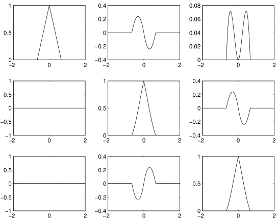
Figure 1: Result after $12$ iterations of the $3\times 3$ non-stationary subdivision scheme in (64).

By construction this scheme satisfies the $V_{2,\lambda}$-spectral condition and according to Theorem 16 it is possible to find a subdivision operator ${\cal S}_{{\boldsymbol{B}}^{[n]}}$ such that the factorization (50) holds true. At the $n$-th iteration, its symbol is given by:

$$\left(B^{[n]}\right)^{*}(z)=\frac{1}{16}\left[\begin{array}[]{ccc}8+8\,z&-4\,\displaystyle{\frac{\sinh\frac{\lambda_{n}}{2}}{\lambda_{n}}}&4\,\displaystyle{\frac{\cosh\frac{\lambda_{n}}{2}-2}{{\lambda_{n}}^{2}}}\\ \vskip 6.0pt plus 2.0pt minus 2.0pt\cr 0&2\,\displaystyle{\cosh\frac{\lambda_{n}}{2}+4\,z}&-2\,\displaystyle{\frac{\sinh\frac{\lambda_{n}}{2}}{\lambda_{n}}}\\ \vskip 6.0pt plus 2.0pt minus 2.0pt\cr 0&-\lambda_{n}\,\sinh\frac{\lambda_{n}}{2}&\cosh\frac{\lambda_{n}}{2}+2\,z\end{array}\right].$$ (66)

The corresponding subdivision scheme seems to be zero-convergent, see Figure 2, and hence contractive as one should expect.

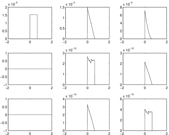
Figure 2: Result after $12$ iterations of the $3\times 3$ non-stationary subdivision scheme based on (66).

To construct the second example, we define the initial sequence of vector data ${\boldsymbol{p}}^{0}=\left([f(\alpha),f^{\prime}(\alpha),f^{\prime\prime}(\alpha),f^{\prime\prime\prime}(\alpha)]^{T}\;:\;\alpha\in\mathbb{Z}\right)$ and apply the same construction as above, just in $V_{3,\Lambda}$.

The symbol at level $n$ can be computed explicitly as

$${\scriptsize\left(A^{[n]}\right)^{*}(z)=\frac{1}{32z}\left[\begin{array}[]{cccc}16\,\left(1+z\right)^{2}&8\,\left(z^{2}-1\right)&\displaystyle{\frac{8}{\lambda_{n}^{2}}\,\left(1+{z}^{2}\right)\left(\cosh\frac{\lambda_{n}}{2}-2\right)}&\displaystyle{\frac{8}{\lambda^{3}}\,{\left(z^{2}-1\right)\left(\lambda+\sinh\frac{\lambda_{n}}{2}\right)}}\\ \vskip 6.0pt plus 2.0pt minus 2.0pt\cr 0&8\,\left(z+1\right)^{2}&\displaystyle{\frac{4}{\lambda_{n}}\left(z^{2}-1\right)\sinh\frac{\lambda_{n}}{2}}&\displaystyle{\frac{4}{\lambda_{n}^{2}}\left(1+{z}^{2}\right)\left(\cosh\frac{\lambda_{n}}{2}-2\right)}\\ \vskip 6.0pt plus 2.0pt minus 2.0pt\cr 0&0&2(1+z^{2})\ \cosh\frac{\lambda_{n}}{2}+8\,z&\displaystyle{\frac{2}{\lambda_{n}}\left(z^{2}-1\right)\ \sinh\frac{\lambda_{n}}{2}}\\ \vskip 6.0pt plus 2.0pt minus 2.0pt\cr 0&0&\lambda_{n}\,\left(z^{2}-1\right)\sinh\frac{\lambda_{n}}{2}&(1+z^{2})\cosh\frac{\lambda_{n}}{2}+4\,z\end{array}\right],}$$ (67)

The determinant of $\left(A^{[n]}\right)^{*}(z)$ factorizes into

$$\det\left(A^{[n]}\right)^{*}(z)=\frac{(z+1)^{4}e^{-\lambda_{n}}\left(e^{\frac{\lambda_{n}}{2}}+z\right)^{2}\left(ze^{\frac{\lambda_{n}}{2}}+1\right)^{2}}{1024\,z^{4}}.$$

Evidence for the convergence of this scheme is given in Fig. 3, where we show the plot of $12$ iterations of the scheme applied to the delta matrix sequence.

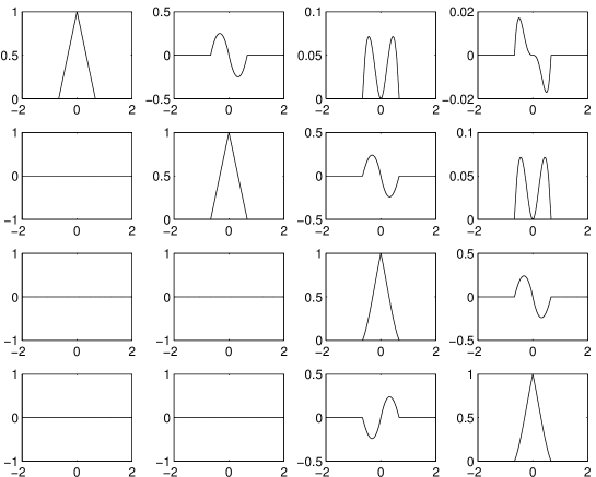
Figure 3: Result after $12$ iterations of the $4\times 4$ non-stationary subdivision scheme based on (67).

This scheme satisfies the $V_{3,\lambda}$-spectral condition and therefore admits the factorization (50) with

$$\left(B^{[n]}\right)^{*}(z)=\frac{1}{32}\left[\begin{array}[]{cccc}16+16\,z&-8&8\,\displaystyle{\frac{\cosh\frac{\lambda_{n}}{2}-2}{{\lambda_{n}}^{2}}}&8\,\displaystyle{\frac{\lambda-\sinh\frac{\lambda_{n}}{2}}{{\lambda_{n}}^{3}}}\\ \vskip 6.0pt plus 2.0pt minus 2.0pt\cr 0&8+8\,z&-4\,\displaystyle{\frac{\sinh\frac{\lambda_{n}}{2}}{\lambda_{n}}}&4\,\displaystyle{\frac{\cosh\frac{\lambda_{n}}{2}-2}{{\lambda_{n}}^{2}}}\\ \vskip 6.0pt plus 2.0pt minus 2.0pt\cr 0&0&2\,\cosh\frac{\lambda_{n}}{2}+4\,z&-2\,\displaystyle{\frac{\sinh\frac{\lambda_{n}}{2}}{\lambda_{n}}}\\ \vskip 6.0pt plus 2.0pt minus 2.0pt\cr 0&0&\displaystyle{\lambda_{n}\,\sinh\frac{\lambda_{n}}{2}}&\displaystyle{\cosh\frac{\lambda_{n}}{2}+2\,z}\end{array}\right],$$ (68)

which again seems to be a contraction, see Figure 4.

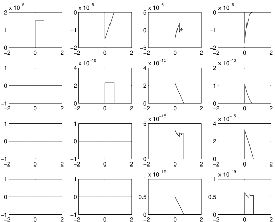
Figure 4: Result after $12$ iterations of the $3\times 3$ non-stationary subdivision scheme based on (68).

We conclude this section by observing that, as $n$ goes to infinity, the symbols $\left(A^{n]}\right)^{*}(z)$ in (65) and (67) tend to

$$\left(A^{[\infty]}\right)^{*}(z)=\frac{1}{16z}\left[\begin{array}[]{ccc}8\,\left(z+1\right)^{2}&4\,\left(z^{2}-1\right)&({z}^{2}+1)\\ \vskip 6.0pt plus 2.0pt minus 2.0pt\cr 0&4\,\left(z+1\right)^{2}&2\,\left(z^{2}-1\right)\\ \vskip 6.0pt plus 2.0pt minus 2.0pt\cr 0&0&2\,\left(z+1\right)^{2}\end{array}\right],$$

and

$$\left(A^{[\infty]}\right)^{*}(z)=\frac{1}{96z}\left[\begin{array}[]{cccc}48\,\left(z+1\right)^{2}&24\,\left(z^{2}-1\right)&6\,({z}^{2}+1)&\left(z^{2}-1\right)\\ \vskip 6.0pt plus 2.0pt minus 2.0pt\cr 0&24\,\left(z+1\right)^{2}&12\,\left(z^{2}-1\right)&3\,({z}^{2}+1)\\ \vskip 6.0pt plus 2.0pt minus 2.0pt\cr 0&0&12\,\left(z+1\right)^{2}&6\,\left(z^{2}-1\right)\\ \vskip 6.0pt plus 2.0pt minus 2.0pt\cr 0&0&0&6\,\left(z+1\right)^{2}\end{array}\right],$$

respectively. These are the symbols of Hermite schemes satisfying a polynomial space spectral condition. In particular, they reproduce polynomials up to the degree 2 and 3, respectively.

References

[1] M. Charina, C. Conti, L. Romani,
Reproduction of exponential polynomials by multivariate
non-stationary subdivision schemes with a general dilation
matrix, Numer. Math. (2013), in print.
DOI 10.1007/s00211-013-0587-8.
[2]C. Conti, L. Romani, Algebraic
conditions on non-stationary subdivision symbols for exponential
polynomial reproduction, J. Comput. Appl. Math. 236,
(2011), 543–556.
[3]C. Conti, J.L. Merrien, L. Romani,
Dual Hermite Subdivision Schemes of de Rham-type, preprint.
[4]
S. Dubuc and J.-L. Merrien, Convergent vector and Hermite
subdivision schemes, Constr. Approx. 23 (2006), 1–22.
[5]
S. Dubuc and J.-L. Merrien, Hermite subdivision schemes and
Taylor polynomials, Constr. Approx. 29 (2009),
219–245.
[6]
R. W. Hamming, Digital filters, Prentice–Hall, 1989, Republished by
Dover Publications, 1998.
[7]
J.-L. Merrien and T. Sauer, From Hermite to stationary subdivision
schemes in one and several variables, Advances Comput. Math. 36
(2012), 547–579.
[8]
C. A. Micchelli, Interpolatory subdivision schemes and wavelets, J.
Approx. Theory 86 (1996), 41–71.
[9]
M. Unser and Th. Blu, Cardinal Exponential Splines: Part I —
Theory and Filtering Algorithms, IEEE
Trans. Sig. Proc. 53 (2005), 1425–1438.