Classical spin models

How soon after a zero-temperature quench is the fate of the Ising model sealed?

Abstract

We study the transient between a fully disordered initial condition and a percolating structure in the low-temperature non-conserved order parameter dynamics of the bi-dimensional Ising model. We show that a stable structure of spanning clusters establishes at a time $t_{p}\simeq L^{\alpha_{p}}$. Our numerical results yield $\alpha_{p}=0.50(2)$ for the square and kagome, $\alpha_{p}=0.33(2)$ for the triangular and $\alpha_{p}=0.38(5)$ for the bowtie-a lattices. We generalise the dynamic scaling hypothesis to take into account this new time-scale. We discuss the implications of these results for other non-equilibrium processes.

Phase ordering kinetics is the process whereby an open classical system locally orders in its equilibrium states. This phenomenon occurs when a macroscopic system is taken across a second order phase transition by changing (slowly or abruptly) one of its parameters or the environmental conditions. Theoretic and numeric approaches to phase ordering kinetics focus on the scaling regime, in which structures with typical linear size $\xi(t)$ satisfying $\xi_{micro}\ll\xi(t)\ll L$, with $\xi_{micro}$ a microscopic lenght-scale associated to the lattice spacing and $L$ the linear size of the system, have established. The mechanism controlling the local growth of the equilibrium phases can in general be identified, and allows one to deduce the time-dependence in $\xi(t)$ [1]. The stochastic evolution of the ferromagnetic Ising model (IM) quenched below $T_{c}$ is a textbook example of coarsening phenomenology, with $\xi(t)\sim t^{1/z}$ and $z=2$ for non-conserved order-parameter dynamics [1]. The role played by the initial conditions and the pre-asymptotic dynamics leading to the scaling regime, and atypical ordered spatial regions, in this and other models have not been studied in detail yet.

Evidence for percolation [2] influencing the scaling regime and asymptotic states reached by the $2d$ square-lattice IM after a quench from high to low temperature were given by two groups. In one set of studies, it was shown that, after a very short time span (a few Monte Carlo (MC) steps for the simulated cell), a paramagnetic (PM) configuration quenched sub-critically looks like critical percolation. More precisely, the morphological and statistical properties of structures (areas of domains, lengths of interfaces, etc.) that are larger than the typical ones ($\xi^{d}(t)$, $\xi^{d-1}(t)$, etc.) are the ones of site percolation at its threshold [3, 4]. In the other set of studies, simulations of zero-temperature quenches demonstrated that the systems often block into stripe states [5, 6, 7]. The probabilities of reaching such states were shown to equal, with high numerical precision, the ones of having a spanning cluster at critical percolation [5, 6]. As the occupation probability for up and down spins in a high-$T$ equilibrium configuration is smaller than the one at critical percolation, this fact suggests that the system must have reached critical percolation at some point.

Initial states linked to a different equilibrium fixed point are the critical temperature ones. Studies of quenches from $T_{c}$ into the ordered phase along the lines above were also performed. Large structures are, in this case, characteristic of the critical Ising point [3, 4]. Moreover, the blocked states reached at $T=0$ appear with probabilities dictated by the ones of the critical Ising spanning structures [7].

In this work we analyze the transient regime between the initial condition and the state that will actually control the large scale properties in the scaling regime and the eventually frozen asymptotic configurations. We study the $2d$IM on different lattices. High-$T$ and critical Ising initial conditions are considered. We determine the dependence of the time-scale needed to reach this state, that we call $t_{p}$, on the lattice coordination and the system size by analyzing how $t_{p}$ manifests itself in a number of non-trivial observables. We conjecture its dependence on the microscopic dynamics. Importantly enough, we generalize the dynamic scaling framework to include the influence of this time-scale, so-far ignored, on the dynamic correlations. Finally, we discuss the possible implications of our results on systems with more complex out of equilibrium dynamics.

We consider the ferromagnetic Ising model defined by

$$H=-J\sum_{\langle ij\rangle}S_{i}S_{j},$$ (1)

where the sum is restricted to nearest neighbors on a $2d$ lattice. We fix $J=1$, and $S=\pm 1$. The system undergoes a continuous phase transition at a lattice-dependent critical temperature $T_{c}$. We consider square, triangular, kagome and bowtie-a lattices with linear size $L$ and either free (FBC) or periodic (PBC) boundary conditions. The coordination numbers are $n_{c}^{\square}=4$, $n_{c}^{\triangle}=6$, $n_{c}^{K}=4$, and $n_{c}^{\bowtie}=5$ and the site percolation thresholds are $p^{\square}_{c}\simeq 0.59$, $p^{\triangle}_{c}=0.5$, $p^{K}_{c}\simeq 0.65$ and $p_{c}^{\bowtie}\simeq 0.55$. $n_{c}^{\bowtie}$ is a mean coordination number since the sites have either $4$ or $6$ neighbors on this lattice. (Regularly odd-coordinated lattices are not suited for our study because the evolution rapidly freezes due to metastable droplets [8]; lattices such that $p_{c}<1/2$ are not either because the initial state is super-critical.)

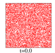
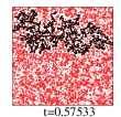
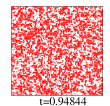
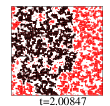
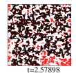
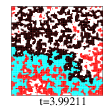
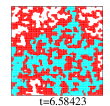
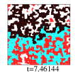
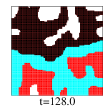
Figure 1: (Color online.) Snapshots of a $2d$IM on a square lattice with $L=128$ and FBC. A quench from $T_{i}\to\infty$ to $T=0$ was performed at $t=0$. Spins $S_{i}=-1\ (S_{i}=+1)$ are shown in red (white). A percolating cluster of spins $S_{i}=-1$ ($S_{i}=+1$) is shown in black (clear blue).

We focus on instantaneous quenches from infinite to a sub-critical temperature. The initial PM state is a random configuration with $S_{i}=\pm 1$ with probability a half. The dynamics follow the MC rule. $L^{2}$ spin-flip attempts correspond to $\delta t=1$. At $T<T_{c}$, the number of flippable spins decreases with time so we accelerate our simulations with a Continuous Time MC algorithm [9]. Unless otherwise stated the number of samples used is at least $10^{6}$.

The equilibration time $t_{eq}$ is estimated from $\xi(t_{eq})\sim L$ and yields $t_{eq}\sim L^{2}$. After $t_{eq}$, the configuration is in one ergodic component, or it is a stripe state with interfaces crossing the lattice. The stripes are stable or not depending on the lattice and boundary conditions. Unstable stripes are destroyed via a different mechanism over a much longer time-scale [10, 11].

Let us start by analysing the dynamics of the square lattice model. A glimpse on a set of snapshots taken at and after the quench shows that, although there are no percolating clusters in the initial state, these appear very soon. Figure 1 displays the configurations of a system with $L=128$ and FBC quenched from $T_{i}\to\infty$ to $T=0$. At $t=0$ the spins take random values and no spanning cluster is present. At $t_{f}\simeq 0.57\ll L^{2}$ a first spanning cluster appears. Then follows a period $t_{f}<t<t_{p}$ with $t_{p}\simeq 7.46\ll L^{2}$ in which spanning clusters appear and disappear typically $10$ to $20$ times in our simulations. At $t_{p}$ the number and type of spanning clusters are equal to the number and kind of stripes in the final state. The fact that $t_{p}\ll L^{2}$ is intriguing as it indicates that the fate of the Ising model is sealed very soon in the evolution. The regime $t_{f}<t<t_{p}$ is also interesting but we will not consider it here.

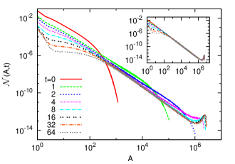
Figure 2: ${\cal N}(A,t)$ vs. $A$ at different times $t$ given in the key after a quench from $T_{i}\to\infty$ to $T_{c}/2$ for a system with $L=2560$. In the inset data obtained after a quench from $T_{c}$ to $T_{c}/2$.

A first quantitative indication of critical percolation playing a role is given by the probability distribution of spin cluster areas, ${\cal N}(A,t)$, as a function of the number of spins in a cluster, $A$, and time, $t$ [3, 4]. At $t=0$ the system is not critical and ${\cal N}(A,0)$ decays exponentially with $A$, as shown by the solid (red) curve in the main panel in Fig. 2. After a very short time, $t\simeq 10$, the tail tends to an algebraic decay ${\cal N}(A,t)\simeq 2cA^{-\tau}$. For finite $L$ and sufficiently long times the power-law is cut-off by a bump around areas that scale with $L$. For $t\gtrsim 16$ the power-law holds in the range $10^{3}\leq A\leq 10^{6}$ and the bump is around $A\simeq 2\ 10^{6}$. The functional form

$${\cal N}(A,t)\simeq 2cA^{-\tau}+N_{p}(A/L^{D},t)$$ (2)

takes into account all these features. $D=d/(\tau-1)$ is the fractal dimension of the percolating clusters.

A direct fit of the power-law yields $\tau=2.020-2.040$ depending on the fitting range. While these values are close to the percolation one, $\tau=187/91\simeq 2.05495$, they are also close to the critical $2d$IM one, $\tau=2.02674$, and it is difficult to distinguish between these two cases with this measurement (having said this, the numerical value of $c$ is very close to the analytic one for percolation, $c=1/(8\sqrt{3}\pi)$ [12] and distinctively different from the one for the critical IM [3, 4]).

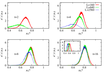
Figure 3: (Color online.) $A^{\tau}{\cal N}(A,t)$ vs. $A/L^{D}$ at different times $t$ after a quench from $T_{i}\to\infty$ to $T_{c}/2$. We employ the parameters $\tau$ and $D$ of critical percolation except in the inset of the lower right panel where we use the ones of the critical Ising model. The number of samples used to build the pdf is $10^{6}$ for $L=160$ and $L=640$ and $2\ 10^{5}$ for $L=2560$.

The study of the bump, scaled as in the second term in (2), lifts all ambiguities on the value of $\tau$. In Fig. 3 we plot $A^{\tau}{\cal N}(A,t)$ vs. $A/L^{D}$ with the percolation $\tau$ for $t\in[2,16]$ and different $L$. For small $t$ the height of the distribution depends on $L$ while for $t\gtrsim 16$ they all collapse. The inset in the lower right panel displays the same data scaled with the critical IM value of $\tau$. Clearly, there is no scaling with this choice.

We note that the time required for the distribution to become percolation-like increases weakly with $L$. The curves for $L=160$ and $L=640$ at $t=2$ are replaced by the curves for $L=640$ and $L=2560$ at $t=4$. The same holds true between $t=4$ and $t=8$. At $t=8$, the curves for $L=160$ and $L=640$ do collapse, as for data at $t=16$ for $L=640$ and $L=2560$. This suggests that there is a time scale $t_{p}\sim L^{\alpha_{p}}$, with $\alpha_{p}\sim 0.5$, after which the bump remains stable in the scaling plot. It is still not clear whether this bump is made of everlasting percolating structures or whether these still appear and disappear as illustrated in Fig. 1.

The time-scale $t_{p}$ after which the actual percolating structure stabilizes can be estimated from the analysis of the correlation of the number of crossing clusters present at time $t$ and those surviving in the blocked configuration at zero temperature:

$${\cal A}_{c}(t)=\langle\delta_{n_{v}(t)n_{v}^{\infty}}\delta_{n_{h}(t)n_{h}^{\infty}}\rangle\;.$$ (3)

We note $n_{h}(t)$ [$n_{v}(t)$] the number of horizontal (vertical) crossing clusters at time $t$, $n_{h}^{\infty}\ (n_{v}^{\infty})$ the number of horizontal (vertical) spanning clusters in the blocked configuration, $\langle\cdots\rangle$ the average over initial configurations and thermal histories, and $\delta_{ab}$ the Kronecker delta. For geometrical reasons the clusters crossing in only one direction must be at least two in the final state so that if $n_{h}(t)=0$ and $n_{v}(t)>0$ then $n_{v}(t)\geq 2$. A cluster crossing in both directions is always unique and $n_{h}(t)=n_{v}(t)=1$. For a configuration with no crossing clusters $n_{h}(t)=n_{v}(t)=0$.

The correlation ${\cal A}_{c}(t)$ interpolates between $0$ and $1$. For sufficiently large system sizes, $n_{h}(0)=n_{v}(0)=0$. In the blocked configuration there should be at least one crossing cluster, leading to $n_{h}^{\infty}\neq 0$ and/or $n_{v}^{\infty}\neq 0$. In Fig. 4 we show ${\cal A}_{c}(t)$ on a square lattice with FBC. A very accurate data collapse for different sizes is found for $t/L^{0.5}\gtrsim 0.1$. At shorter times the scaling is not as good due to the large number of states with only one cluster percolating in one direction (see Fig. 1) present on the square lattice because of interface corners. As soon as interfaces become flat these configurations no longer exist. The convergence to $1$ is fast since ${\cal A}_{c}(t)\sim 1$ for $t/L^{0.5}>10$. This indicates that $t_{p}$ scales as $t_{p}\sim L^{0.5}$ on the square lattice.

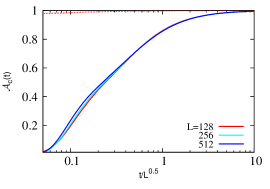
Figure 4: (Color online.) Number of crossings autocorrelation, ${\cal A}_{c}(t)$ defined in Eq. (3), after a quench of the FBC square lattice form $T_{i}\to\infty$ to $T=0$. Data are displayed as a function of $t/L^{0.5}$ in linear-log scale for the values of $L$ given in the key. The dashed red line very close to $1$ is the behavior of ${\cal A}_{c}(t)$ for a quench from $T_{c}$ to $T=0$ for $L=128$.

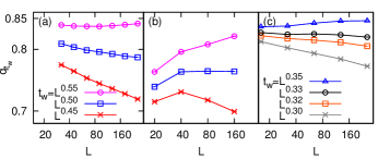
Figure 5: (Color online.) The $L$-dependence of the asymptotic overlap $\lim_{t\to\infty}q_{t_{w}}(t,L)$ in the $2d$IM quenched from a PM state to $T=0$ at $t=0$. (a) Square lattice with FBC. (b) kagome lattice with FBC. (c) Triangular lattice with PBC. The values of $t_{w}(L)$ are given in the keys. Data have been averaged over $10^{6}-10^{7}$ samples.

The overlap between two copies of the system [13, 15, 16, 14] defined as follows also informs us about the time $t_{p}$. At $t=t_{w}$ one makes two copies of the configuration, say $s_{i}(t_{w})=\sigma_{i}(t_{w})$, and lets them evolve with different noises. The overlap between the clones at time $t$ is

$$q_{t_{w}}(t,L)=\frac{1}{N}\sum_{i}\langle s_{i}(t)\sigma_{i}(t)\rangle\;,$$ (4)

where the angular brackets indicate an average over different realizations of this procedure. The two-time scaling properties of this quantity, in the limit $L\to\infty$, were used to distinguish domain-growth processes from glassy ones [15, 16]. It was recently shown that $q_{t_{w}=0}(t,L)$ and $q_{t_{w}=0}(\infty,L)$ decrease algebraically with $t$ and $L$, respectively [14]. The fact that $q_{t_{w}=0}(t,L)$ decreases with $t$ is clear. Even though we know that there are a finite amount of stripes in the final state [5, 6], these are not encoded in the initial condition and there is no reason why the different thermal histories will take the two clones to the same percolating state. Instead, by letting $t_{w}$ go beyond $t_{p}$, the two clones should be strongly correlated for all subsequent times since they are in the same percolating state. We set this argument in practice by computing $\lim_{t\to\infty}q_{t_{w}}(t,L)$ for various $t_{w}(L)$. The outcome is shown in Fig. 5 for the square (a), kagome (b), and triangular $($c$)$ lattices. For the square and kagome lattices, we observe that if $t_{w}(L)$ increases as $L^{0.5}$, the overlap remains constant with a finite value, thus confirming that $t_{p}\sim L^{0.5}$ in these cases.

On the triangular lattice $p^{\triangle}_{c}=1/2$ and there is a percolating cluster in the initial condition with non-zero probability. A naive guess would be that this percolating state survives after the quench, and $t_{p}\equiv 0$. This, however, is not true as $q_{0}(t,L)$ decays to zero in the large size and time limit [17]. As shown in panel (c) in Fig. 5, only for $t_{w}>t_{p}\simeq L^{0.33}$, $\lim_{t\to\infty}q_{t_{w}}(t,L)$ saturates. The initial state, although percolating, is not stable under the dynamics and a transient scaling with $L$ is still needed to reach the truly stable one [18]. We have also simulated the bowtie-a lattice (not shown) and found $t_{p}\sim L^{0.38(5)}$. We have checked that in all the lattices studied the constant prefactor in $t_{p}$ is of order $1$.

These results suggest that, after a sub-critical quench from $T_{i}\to\infty$,

$$t_{p}\simeq L^{\alpha_{p}}\;,\;\;\;\;\;\;\;\;\alpha_{p}=z/n_{c}\;,$$ (5)

with $z$ the dynamic exponent and $n_{c}$ the regular or averaged lattice coordination.

For the system sizes commonly used in the literature $L\simeq 100-1000$, $t_{p}\simeq 10-30$, and percolation is very quickly attained. It is important to notice that, since the equilibration time remains at least $t_{eq}\sim L^{2}\gg t_{p}$ [1], or even longer due to blocked states [10, 11], after stable percolation of an ordered cluster is established at $t_{p}$ the systems are still far from equilibrium, as shown by the correlation and response functions that continue to relax well beyond this time-scale [19, 20]. The new feature provided by our study is that the scaling properties are modified by the extra time-scale $t_{p}$. Indeed, according to the usual formulation of the dynamical scaling hypothesis, in the regime $\xi_{micro}\ll\xi(t)\ll L$, when $\xi$ is grown much larger than a microscopic length $\xi_{micro}$ associated to the lattice spacing but is still much smaller than the system size when equilibration or blocked states start to occur, the statistical properties do not depend on time provided that distances are measured in units of the dominant length $\xi(t)$. Due to this fact, correlators such as $G(r,t)=\langle S_{i}(t)S_{j}(t)\rangle$, where $r=|i-j|$, take the scaling form

$$G(r,t,L)=f\left[\frac{r}{\xi(t)}\right],$$ (6)

where $f(x)$ is a scaling function, expressing the fact that there is a unique relevant length in the system. However, the presence of $t_{p}$ introduces another characteristic length ${\cal L}(L)=\xi(t_{p})\simeq L^{\alpha_{p}/z}$ separating an early stage in which there are no stable percolating structures from a late stage in which they exist. In the presence of two characteristic lengths, since ${\cal L}$ plays a companion role to that of $\xi$, the proper scaling form for $G(r,t,L)$ should read

$$G(r,t,L)=g\left[\frac{r}{\xi(t)},\frac{{\cal L}(L)}{\xi(t)}\right]$$ (7)

with a new, two-variable, scaling function $g(x,y)$. The difference between Eqs. (6) and (7) is manifest when trying to collapse data for $G(r,t,L)$ at different times $t$. Indeed, according to Eq. (7) curves for a system of a given size $L$ (and hence a given ${\cal L}$) cannot be superimposed on a master-curve by simply plotting them against $r/\xi(t)$, as Eq. (6) would suggest, because in so doing the second argument entering the scaling function $g$ changes. Instead, Eq. (7) states that it is possible to collapse curves at different times $t=t_{0},t_{1},\dots,t_{i},\dots$ if they are relative to systems of different sizes $L=L_{0},L_{1},\dots,L_{i},\dots$ chosen in such a way that ${\cal L}(L_{i})/\xi(t_{i})=const.$, by still plotting them against $r/\xi(t)$.

In order to check this we have computed $G(r,t,L)$ on square lattices of sizes $L_{i}=2^{i}\cdot L_{0}$, with $L_{0}=50$ and $i=0-4$. Using Eq. (5) and $\xi(t)\sim t^{1/z}$ leads to ${\cal L}(L_{i})\simeq L_{i}^{1/n_{c}}$. We have considered times $t_{i}$ such that $t_{0}=15$ and ${\cal L}(L_{i})/\xi(t_{i})\simeq 16.86$. Having verified that, for these times, the scaling condition $\xi_{micro}\ll\xi(t)\ll L$ is met for any $L_{i}$, we try to collapse the data for the smaller system according to Eq. (6), namely by simply plotting the data against $r/\xi(t)$ (where $\xi$ is obtained as the half-height width of $G$, namely from the condition $G(\xi,t)\equiv 1/2$). The result is shown in Fig. 6 (a), where one observes a systematic downward spreading of the curves from $r/\xi(t)\simeq 1.5$ onwards (the collapse of the curves at $r/\xi=1$ is exact due to the operative definition of $\xi(t)$). In Fig. 6 (b), instead, we plot the data at the same times $t_{i}$ but for systems with different sizes $L_{i}$. As expected, the quality of the collapse is, in this case, much better. Besides shading some light on the scaling properties of coarsening systems, this results confirm the validity of Eq. (5) in an independent way.

We repeated the analysis for various choices of the constant ${\cal L}(L_{i})/\xi(t_{i})$ finding that, in all cases, Eq. (7) provides a better description of data than Eq. (6), although it is clear that for times $t\gg t_{p}$ (so that $\xi(t)\gg{\cal L}(L)$) the validity of Eq. (6) gets progressively restored since one expects $\lim_{y\to 0}g(x,y)\simeq g(x,0)=f(x)$. We have also checked that, similarly to what happens for $G$, a better scaling description of other correlators, such as, for instance, the autocorrelation function $C(t,t_{w},L)=\langle S_{i}(t)S_{i}(t_{w})\rangle$, can be obtained by taking into account the presence of $t_{p}$. Indeed, also for this quantity we have found that a two-variable scaling form $C(t,t_{w},L)=h\left[\frac{\xi(t_{w})}{\xi(t)},\frac{{\cal L}(L)}{\xi(t)}\right]$ improves the collapse with respect to the usually conjectured form where the role of the second argument in $h$ is neglected.

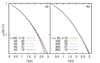
Figure 6: (Color online.) $G(r,t,L)$ against $r/\xi(t)$ in the $2d$IM quenched from a PM state to $T=0$ at $t=0$. The system size and measuring times are given in the keys. Data have been averaged over $2\cdot 10^{4}$ samples.

The situation is different if we start from a configuration equilibrated at $T_{c}$. The inset in Fig. 2 shows ${\cal N}(A,t)$ after a quench from $T_{c}$ to $T_{c}/2$. In this case, the initial state is critical and the curve at $t=0$ is a power law [3, 4]. Again, extracting $\tau$ from it is hard. Instead, the bump described by the second term in (2) can only be scaled by using the critical IM $\tau$ (not shown). Moreover, the crossing properties of the final state are already contained in the initial configuration [7]. ${\cal A}_{c}(t)$ is immediately close to one, see the red dashed line in Fig. 4, as well as the clone overlap $q_{t_{w}}(t,L)$ (not shown).

These results raise many questions. We expect the effect of the working temperature to be weak and alter only the pre-factor in (5). The effect that the microscopic dynamics (conserved quantities) may have on $t_{p}$ remains to be clarified. Weak quenched disorder slows down the curvature driven growth. Does it also affect the transient regime? It would also be interesting to pinpoint the implications of these results in higher dimensions.

It should be possible to search for percolation effects experimentally in systems undergoing phase ordering kinetics for which visualization techniques have proven to be successful. Two examples are liquid crystals [21] and phase separating glasses [22].

References

- [1] A. J. Bray, Adv. Phys. 43, 357 (1994).
- [2] D. Stauffer and A. Aharony, Introduction to Percolation Theory, 2nd ed. (Taylor & Francis, London, 1994).
- [3] J. J. Arenzon, A. J. Bray, L. F. Cugliandolo, and A. Sicilia, Phys. Rev. Lett. 98, 145701 (2007),
- [4] A. Sicilia, J. J. Arenzon, A. J. Bray, and L. F. Cugliandolo, Phys. Rev. E 76, 061116 (2007).
- [5] K. Barros, P. L. Krapivsky, and S. Redner, Phys. Rev. E 80, 040101 (2009).
- [6] J. Olejarz, P. L. Krapivsky, and S. Redner, Phys. Rev. Lett. 109, 195702 (2012).
- [7] T. Blanchard and M. Picco, Phys. Rev. E 88, 032131 (2013).
- [8] H. Takano and S. Miyashita, Phys. Rev. B 48, 7221 (1993).
- [9] A. B. Bortz, M. H. Kalos, and J. L. Lebowitz, J. Comp. Phys. 17, 10 (1975).
- [10] A. Lipowski, Physica A, 268, 6–13 (1999).
- [11] V. Spirin, P. L. Krapivsky, and S. Redner, Phys. Rev. E 63, 036118 (2001), Phys. Rev. E 65, 016119 (2001).
- [12] J. Cardy and R. M. Ziff, J. Stat. Phys. 110, 1 (2003).
- [13] B. Derrida, J. Phys. A 20, L721 (1987).
- [14] J. Ye, J. Machta, C. M. Newman, and D. L. Stein, Phys. Rev. E 88, 040101(R) (2013).
- [15] L. F. Cugliandolo and D. S. Dean, Phys. A 28, 4213 (1995).
- [16] A. Barrat, R. Burioni, and M. Mézard, J. Phys. A 29, 1311 (1996).
- [17] T. Blanchard, L. F. Cugliandolo, and M. Picco, in preparation.
- [18] See Supplementary Material for snapshots of the evolution of a system on a triangular lattice.
- [19] A. Barrat, Phys. Rev. E 57, 3629 (1998).
- [20] F. Corberi, E. Lippiello, A. Sarracino, and M. Zannetti, J. Stat. Mech. P04003 (2010).
- [21] A. Sicilia et al., Phys. Rev. Lett. 101, 197801 (2008).
- [22] D. Bouttes et al., arXiv:1309.1724.