Star formation in the cluster CLG0218.3-0510 at z=1.62 and its large-scale environment: the infrared perspective

Abstract

The galaxy cluster CLG0218.3-0510 at $z$=1.62 is one of the most distant galaxy clusters known, with a rich muti-wavelength data set that confirms a mature galaxy population already in place. Using very deep, wide area (20$\times$20 Mpc) imaging by Spitzer MIPS at 24$\mu m$, in conjunction with Herschel 5-band imaging from 100–500$\mu m$, we investigate the dust-obscured, star-formation properties in the cluster and its associated large scale environment. Our galaxy sample of 693 galaxies at $z\sim$1.62 detected at 24$\mu m$ (10 spectroscopic and 683 photo-$z$) includes both cluster galaxies (i.e. within $r<$1 Mpc projected clustercentric radius) and field galaxies, defined as the region beyond a radius of 3 Mpc. The star-formation rates (SFRs) derived from the measured infrared luminosity range from 18 to 2500 M_⊙/yr, with a median of 55 M_⊙/yr, over the entire radial range (10 Mpc). The cluster brightest FIR galaxy, taken as the centre of the galaxy system, is vigorously forming stars at a rate of 256$\pm$70 M_⊙/yr, and the total cluster SFR enclosed in a circle of 1 Mpc is 1161$\pm$96 M_⊙/yr. We estimate a dust extinction of $\sim$ 3 magnitudes by comparing the SFRs derived from [OII] luminosity with the ones computed from the 24$\mu m$ fluxes. We find that the in-falling region (1–3 Mpc) is special: there is a significant decrement (3.5$\times$) of passive relative to star-forming galaxies in this region, and the total SFR of the galaxies located in this region is lower ($\sim$130 M_⊙/yr/Mpc²) than anywhere in the cluster or field, regardless of their stellar mass. In a complementary approach we compute the local galaxy density, $\Sigma_{5}$, and find no trend between SFR and $\Sigma_{5}$. However, we measure an excess of star-forming galaxies in the cluster relative to the field by a factor 1.7, that lends support to a reversal of SF–density relation in CLG0218.

1 Introduction

One of the main concerns of modern astrophysics is the lack of a detailed understanding of galaxy formation in a cosmological context. The star-formation rate (SFR) of galaxies in different environments and across cosmic time is one of the key physical parameters to understand their evolution.

In the local universe, luminous infrared galaxies (LIRGs, 10${}^{11}<L_{IR}<$10¹² L_⊙) avoid the high-density environments of galaxy clusters in which star formation has already been quenched, and ultra luminous infrared galaxies (ULIRGs, $L_{IR}>$10¹² $L_{\odot}$) are virtually absent up to $z\sim$0.5 (e.g., Magnelli et al., 2011; Haines et al., 2013). Since the peak of the cosmological star-formation rate occurred at 1 $<z<$ 3 (Madau et al., 1996), it is expected that star formation in the denser environments must at some time increase towards higher redshifts. However, the amount, spatial distribution, and timing of this increase remains unclear.

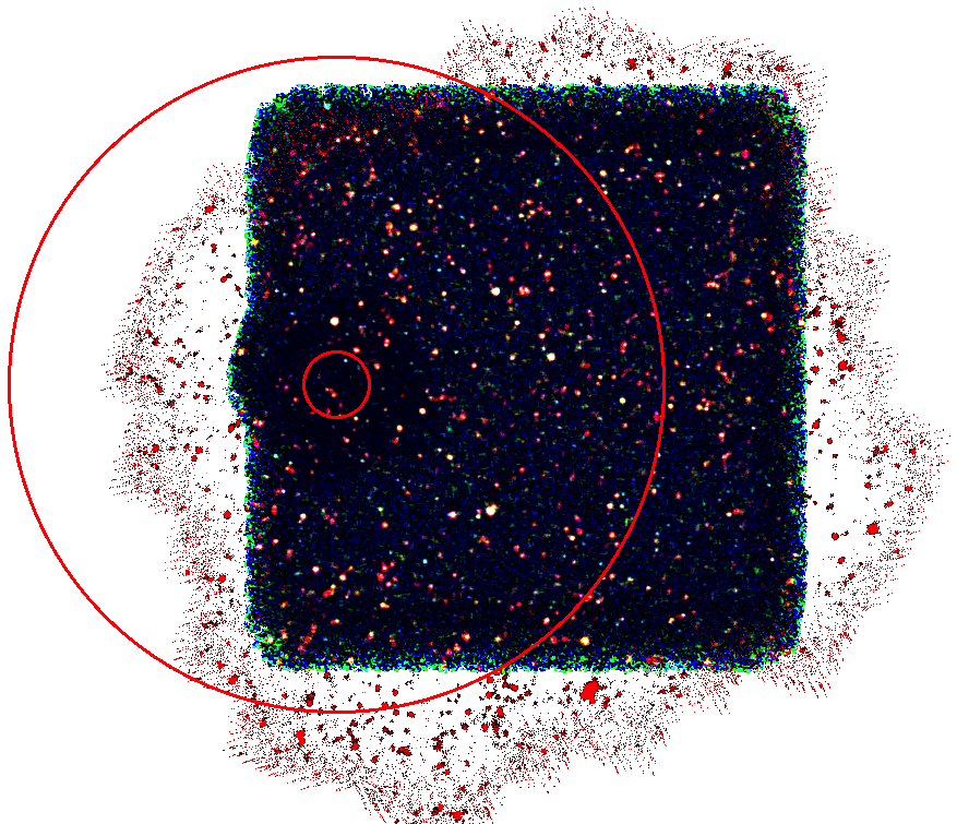
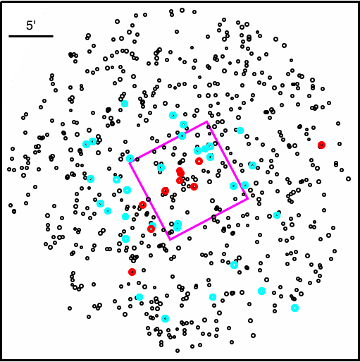
Figure 1: (Left) Colour image (250/160/100 $\mu m$) of the Herschel co-added observations of CLG0218. The inner red circle is centered on the galaxy ID 16 and has a radius of 2$\arcmin$. The larger circle with $r$=10 Mpc encloses the area covered by the MIPS catalogue used in this work. (Right) Footprint of cluster members with MIPS detection in a 10 Mpc radius area centered on the cluster galaxy ID 16. Photometric redshift galaxies with $z_{phot}$= 1.52-1.72 are shown in black, spectroscopic galaxies in red and $z_{phot}$ galaxies with [OII] narrow band emission in cyan. The magenta 10$\arcmin\times$10$\arcmin$ square corresponds to the area with deep PACS imaging.

The evolution of the star-formation rate with redshift has been studied up to $z\sim$1 and is typically parametrized by a power-law function, SFR($z$) $\propto$ (1+$z$)^α, with a slope $\alpha$ ranging from 2 to 7 (e.g., Kodama et al., 2004; Geach et al., 2006; Saintonge et al., 2008; Bai et al., 2009; Haines et al., 2009). The recent investigation of Webb et al. (2013) using 42 clusters from the Red Sequence Cluster Survey lends support to a slope of 5–6 and ascribes this evolutionary trend to the in-falling galaxies in clusters at $z>$ 0.75. This conclusion underlines the importance of environment as we probe higher redshifts. Beyond redshift unity the evolution of the SFR in clusters is unconstrained mostly because of the scarcity of well studied systems (i.e., few confirmed clusters with good multi-wavelength data), however the recent works of (Brodwin et al., 2013; Zeimann et al., 2013) made a first step in that regime.

A reversal of the star formation–density relationship at $z>$ 1 was reported by Elbaz et al. (2007, 2011) in low galaxy density environments (i.e. the field) where, unlike in the local Universe, the average star-formation rate of galaxies increases with local galaxy density. On the other hand, mid-infrared observations of a couple of galaxy clusters at the highest known redshifts ($z\sim$ 1.5) have revealed a population of IR luminous, actively star-forming galaxies in the cluster cores (Hilton et al., 2010; Tran et al., 2010), indicating a reversal of the SF–density relation in higher galaxy density systems.

At intermediate and high-redshifts most of the energy from star formation and AGN activity is absorbed by dust and re-radiated at IR wavelengths. The Infrared Space Observatory (ISO) revealed that in intermediate redshift clusters most of the star formation is hidden at optical wavelengths (e.g., Duc et al., 2002; Metcalfe et al., 2005). Subsequent observations with Spitzer/MIPS confirmed this scenario (e.g., Geach et al., 2006; Marcillac et al., 2008). Specifically, Saintonge et al. (2008) observed an increasing fraction of dusty star-forming cluster galaxies from 3% locally to 13% at $z$ = 0.83 (see also Haines et al., 2009). In addition, it has been shown that most of the dust-obscured star formation in z $<$ 0.85 clusters happens in intermediate density regions (Koyama et al., 2008) or in groups (Tran et al., 2009).

The Herschel space observatory (Pilbratt et al., 2010) is the largest space telescope to date and provides unrivalled sensitivity in the wavelength range 55 to 672$\mu m$. Therefore, Herschel brackets the critical peak of FIR emission of $z\sim$1-2 galaxies, providing a direct, unbiased measurement of star formation. Up to now only a handful of studies of high-$z$ clusters and proto-clusters using Herschel data have been published (Popesso et al., 2012; Seymour et al., 2012; Santos et al., 2013; Pintos-Castro et al., 2013; Alberts et al., 2013), mostly because the angular resolution at the longest wavelengths (up to 18$\arcsec$) does not allow one to resolve small distant galaxies, and furthermore most of the observations have a high SFR detection threshold, enabling the study of the highly star-forming galaxies only. To investigate the relation between star-formation activity and environment at the epoch when clusters are assembling galaxies and galaxies are still undergoing their own formation process, several Herschel programmes, namely the Key Project PEP (PACS Evolutionary Probe, Lutz et al., 2011), and several guaranteed time (GT, PI Altieri) and open time (OT) programmes (PI Pope, Popesso) have targeted several tens of high-redshift clusters in a broad range of halo masses.

In this paper we present a detailed characterization of the infrared star-formation properties in the galaxy population of CLG0218.3-0510 (hereafter CLG0218, RA=34.59955 DEC= -5.17385) at $z$=1.62 and its large scale environment. This distant galaxy system was independently discovered as a strong overdensity of red galaxies using Spitzer-IRAC imaging (Papovich et al., 2010) and as a weak X-ray detection in XMM-Newton data (Tanaka et al., 2010). Subsequently, CLG0218 was observed with deep, multi-wavelength follow-up observations using the major astronomical observatories, in particular the Spitzer public legacy survey (SpUDS, PI: Dunlop) and the Cosmic Assembly Near-Infrared Deep Extragalactic Legacy Survey (CANDELS, PIs Faber, Ferguson). While the number of confirmed cluster members has been steadily increasing with a current sample of $\sim$ 50 galaxies (Papovich et al., 2010; Tanaka et al., 2010; Tadaki et al., 2012), the analysis of 85 ksec X-ray Chandra (Pierre et al., 2012) data rendered inconclusive whether there is extended emission associated with the galaxy overdensity, mostly because a bright point source associated with the central cluster galaxy dominates the X-ray flux. Removing this point source an upper limit on the cluster mass of 7.7$\times$10¹³M_⊙ was set, placing CLG0218 in the low mass / group category, or even proto-cluster. This value is consistent with the one derived from the deeper XMM-Newton data published in Tanaka et al. (2010), 5.7$\pm$1.4$\times$10¹³M_⊙, which we adopt in this paper. Throughout this paper we will simply refer to CLG0218 as a cluster of galaxies. The star-formation properties of this cluster have been studied using MIPS-24$\mu m$ in a central region of 1 Mpc by Tran et al. (2010). They found an enhancement of the fraction of star-forming galaxies in the cluster relative to lower redshift clusters. One caveat in this study is that the 24$\mu m$ derived SFRs were computed with the Chary & Elbaz (2001) templates which are known to overestimate the SFR for galaxies above $z$=1.5. Tadaki et al. (2012) followed a different approach using near-infrared (NIR) narrow-band imaging targeted to detect [OII] emitters in the cluster and the surrounding environment. They found a large filamentary structure around CLG0218 traced by [OII] emitters with a measured overdensity a factor 10 larger in the high density regions (cluster core and clumps) than in the field.

Here we use the largest sample of $z_{phot}$ and spectroscopically confirmed galaxies, and infrared maps that cover an area of 20$\times$20 Mpc thus enabling the study of the dust-obscured star formation in the cluster and its large scale environment. For a subset of the galaxy sample we have robust Herschel measurements which firmly constrains the amount of dust extinction and validates the star formation rates from 24$\mu m$.

The paper is organized as follows: in §2 we describe the MIPS, PACS and SPIRE observations and reduction procedures while in §4 we describe the multi-$\lambda$ ancillary used in this work. In §5 we obtain total infrared luminosities ($L_{IR}$) and derive star formation rates (SFRs) from the 24$\mu m$ data. A detailed analysis of the infrared properties of the central, IR brightest cluster galaxy is presented in §6. In §7 and §8 we investigate the relations between the environment, stellar mass and star formation. Our conclusions are summarized in §9.

The cosmological parameters used throughout the paper are: $H_{0}$=70 $h$ km/s/Mpc ($h$=1), $\Omega_{\Lambda}$=0.7 and $\Omega_{\rm m}$=0.3. In this cosmology, 1 Mpc at $z$=1.6 corresponds to $\sim$2$\arcmin$ on the sky. Quoted errors are at the 1-$\sigma$ level, unless otherwise stated.

2 Infrared observations and data reduction

2.1 MIPS data and source catalogue

CLG0218 was observed with Spitzer IRAC and MIPS 24$\mu m$ as part of SpUDS. The MIPS source catalogue was obtained with the PSF-fitting code StarFinder (Diolaiti, 2000) on the publicly available SpUDS images. Details on the MIPS source extraction and catalogue production can be found in Tran et al. (2010), that presented a subset limited to an area of 1 Mpc centered on the cluster. For the present work we select all sources detected with S/N $>$ 5 (which corresponds to a flux of 40$\mu$Jy) centered on the galaxy ID 16 (see §6) that is associated with an X-ray point source, out to a projected radius $r$=20$\arcmin$, that corresponds to 10 Mpc at the cluster redshift.

Table 1: Summary of the datasets used in our analysis. The ”Type” column refers to spectroscopy (S) or imaging (I).

Instrument	Type	Observed Band	Field-of-view
IMACS	S	MOS	15.46$\arcmin\times$15.46$\arcmin$
FMOS	S	MOS, $1.6-1.8\mu m$	30$\arcmin\phi$
MOIRCS	S	MOS, $0.9-1.7\mu m$	7$\arcmin\times$4$\arcmin$
MegaCAM	I	u	1 deg$\times$1 deg
SuprimeCAM	I	$BVRiz$	52$\arcmin\times$52$\arcmin$
WFCAM	I	J, H, K	41$\arcmin\times$41$\arcmin$
IRAC	I	3.6/4.5/5.8/8.0 $\mu m$	41$\arcmin\times$41$\arcmin$
MIPS	I	24 $\mu m$	41$\arcmin\times$41$\arcmin$
PACS	I	100/160 $\mu m$	34$\arcmin\times$34$\arcmin$
SPIRE	I	250/350/500 $\mu m$	34$\arcmin\times$34$\arcmin$
ACIS-S	I	0.5-10 keV	8.5$\arcmin\times$8.5$\arcmin$

2.2 Herschel data reduction and photometry

The Herschel 100/160/250/350/500$\mu m$ observations of CLG0218 were carried out as part of several programmes: (i) a 50 h guaranteed time programme (GT1, PI Altieri) aimed at studying the star formation history in high redshift (0.8$<z<$ 2.2) galaxy clusters, (ii) 80 h observations of the CANDELS fields (PI M. Dickinson) and (iii) 25 h observations of the HerMES Key Program (PI S. Oliver). We note that the PACS observations performed by these different programmes cover different areas at different depths. While the GT1 is centered on a 10$\arcmin\times$10$\arcmin$ region around the cluster centre, the deeper CANDELS dataset imaged a larger rectangular area (9$\arcmin\times$20$\arcmin$), and HerMES imaged a much larger area (30$\arcmin\times$30$\arcmin$) but with shallow exposures. See in Figure 1 the co-added image of the 3 programmes. As a consequence, the sensitivity of the PACS images varies significantly across the FOV, however it is optimal in the cluster region (magenta square in Fig. 1 with 10$\arcmin\times$10$\arcmin$). The 3-$\sigma$ sensitivity ranges from 1.3 (3.9) mJy (GT1+CANDELS+HerMES area) to 4.0 (9.6) mJy (HerMES only) in the 100 (160)$\mu m$ image.

The PACS (Poglitsch et al., 2011) GT1 observations at 100/160$\mu m$ were acquired on 19 January 2011 (obsids = 1342213032-5) with 4 crossed scan maps of 2.4h each covering a field of 10$\arcmin\times$10$\arcmin$ and the CANDELS observations on the Ultra Deep Survey (UDS) field were spread throughout July 2012 for a total of 80 h. The data were reduced using Hipe 9 (Ott et al., 2006). The data cubes were processed with a standard pipeline where detector timelines are highpass filtered with a sliding median over 21 readouts at 100$\mu m$ and 41 readouts at 160$\mu m$ to remove detector drifts and 1/f noise, with an iterative masking of the sources.

Given the large PSF / beam sizes of PACS and SPIRE, we opt to extract sources using priors, instead of matching blind catalogues using nearest neighbour approaches. Using our MIPS catalogue as prior we run HIPE/DAOPHOT to extract the sources and perform aperture photometry in the PACS bands. The aperture photometry is corrected with the encircled energy factors given by Balog et al. (2013) in radii of 6$\arcsec$ at 100$\mu m$ and 9$\arcsec$ at 160$\mu m$. Given the difficulty to obtain reliable errors with standard source detection algorithms because of the correlated noise present in PACS data, we compute the photometric errors as the 1-$\sigma$ detection limits in each band, in addition to 7% of the source’s flux. The astrometry relative to MIPS 24$\mu m$ is excellent and no shift was required to be applied to the PACS maps.

For our analysis we used the SPIRE (Griffin et al., 2010) observations at 250, 350 and 500$\mu m$ from Herschel-CANDELS UDS. The Herschel-CANDELS UDS observations are one of the deepest SPIRE observations, at a similar depth to GOODS-N from Herschel-GOODS (Elbaz et al., 2011), achieving instrumental noise much deeper than the nominal SPIRE extragalactic confusion noise (Nguyen et al., 2010). The Herschel-CANDELS UDS observations were performed following an 8-point dithering pattern in order to achieve more homogeneous coverage within the CANDELS UDS area. Adding the shallower smaller area GT1 observations or the HerMES (Oliver et al., 2012) observations in this region does not improve the depth as we are limited by the confusion – it only creates regions of inhomogeneous coverage within the field. The dithering also allows using a smaller than nominal pixel scale. Although this does not improve the resolution (below the Nyquist sampling), it improves the definition of the sources: the maps were made with (3.6,4.8,7.2)$\arcsec$/pixel for (250,350,500)$\mu m$. The rms noise in the three SPIRE bands within the good coverage is (3.3,4.0,5.8)$\times\sim$1.48 mJy at (250,350,500)$\mu m$ and indeed this is similar to the nominal extragalactic confusion noise of (5.8,6.3,6.8) mJy but still within the field-to-field or flux calibration uncertainties.

The SPIRE source detection was performed using Sussextractor (SXT, Smith et al., 2012) with a prior catalogue based on the MIPS+PACS catalogue. SXT finds a maximum likelihood fit of the SPIRE beam at the position of the input catalogue sources in the three bands independently. In each band the quality of the fit (e.g. the signal-to-noise) is a measure of the source detection that we also confirmed by visual inspection. When there was no plausible source at the position of the input catalogue we used the $3\sigma$ upper limit in each band, i.e. three times the confusion noise or (17.4,18.9,20.4) mJy at (250,350,500)$\mu m$.

3 Ancillary data

In addition to the MIPS and Herschel data we use the optical/near-IR imaging and spectroscopy summarized below (see Table 1). Details on the observations and reduction procedures can be found in the appropriate references. When referring to the spectroscopic data we intend the reduced source catalogues obtained in the literature or private communications. We use the optical spectroscopy catalogue of Papovich et al. (2010) obtained with the IMACS instrument at the Magellan telescope, as well as the near-infrared spectroscopy obtained with MOIRCS installed in the Subaru telescope and reported in Tanaka et al. (2010), and with FMOS also on Subaru (Tadaki et al., 2012).

Our optical/near-IR spectral energy distribution (SED) fitting presented below is based on multi-wavelength data collected from a number of surveys. Deep $BVRiz$ imaging has been performed with the Suprime-CAM at Subaru (Furusawa et al., 2008) and we use the publicly available z-band selected catalogue (z_AB=26.5 mag), which forms the basis of our catalogue. We combine this catalogue with the $u$-band photometry taken with CFHT MegaCAM ($u^{*}_{AB}(5\sigma,2"{\rm ap.})=27.0$) by cross-matching objects in the two catalogues within 1 arcsecond. We further include the publicly available $JHK$ photometry from DR8plus taken as part of the UKIRT Infrared Deep Sky Survey (UKIDSS, Lawrence et al. 2007). We use 2$\arcsec$ apertures and apply aperture corrections (which are estimated for each data set) to measure total magnitudes. We note that although the $K$-band would be more appropriate than the z-band to select red (dusty) galaxies at $z$=1.62, the $K$-band data is 1.5 magnitudes shallower than the z-band ($K_{AB}$=25 mag, 3$\sigma$). We performed several checks to assess the z-band versus $K$-band selection using our catalogues and we made SED shape predictions based on the limiting magnitudes of the z- and $K$-bands, using the templates of Berta et al. (2013) shifted to $z$=1.6. We conclude that with the z-band selection we do not significantly miss MIPS sources (7-8% of sources at all redshifts) that would otherwise be detected in the $K$-band, therefore we find that the deep z-band catalogue is suitable for the galaxy selection, in comparison with the shallower $K$-band catalogue. The Spitzer IRAC observations of CLG0218 obtained by the SpUDS are also included in the optical-NIR SED fitting.

The 85 ksec Chandra observation published in Pierre et al. (2012) is also used here. While no diffuse emission was detected in this data, the sub-arcsecond resolution of Chandra allowed for the detection of three point-sources associated with confirmed cluster members which will be important to evaluate the impact of AGN in the IR SEDs.

4 Galaxy cluster sample

As detailed below, our galaxy cluster sample is divided in a more robust, spectroscopically confirmed sample, and a photometric redshift sample of galaxies with 24$\mu m$ emission.

4.1 Spectroscopic galaxies

Our spectroscopic sample of 46 cluster members originates from 3 observation campaigns: (i) the IMACS (Papovich et al., 2010) and (ii) MOIRCS observations (Tanaka et al., 2010) secured 16 cluster members selected by colour and photometric redshifts, and (iii) the more recent large area follow-up with FMOS of [OII] narrow-band emitters (Tadaki et al., 2012) independently confirmed 40 cluster members. Of these, ten galaxies overlap with the initial IMACS + MOIRCS catalogue. A total of ten spectroscopic galaxies extending to a radius of 8.5 Mpc at the cluster redshift have 24$\mu m$ emission and will be used in our investigation of the star formation of the cluster and its associated large scale environment.

Table 2: List of the spectroscopic galaxies at $z$=1.62 (first ten rows) and photo-$z$ candidates with [OII] emission (33 rows after break) from Tadaki et al. (2012) detected by MIPS. The infrared properties are based on the 24$\mu m$ fluxes and corrected for the mid-IR excess problem following the approach of Rujopakarn et al. (2013).

ID	RA	DEC	z	Dist	$M_{*}$	F24	$L_{IR}$	SFR
				(kpc)	($\times$1010 M⊙)	mJy	($\times$1011$L_{\odot}$)	(M⊙/yr)
6*	34.57167	-5.18492	1.6487	915	6.35	0.0793$\pm$0.00269	5.21$\pm$0.34	42.1$\pm$2.9
7	34.59967	-5.15572	1.6222	553	2.20	0.08455$\pm$0.00340	5.62$\pm$0.37	46.9$\pm$3.2
10	34.56325	-5.13664	1.6224	1585	4.69	0.12074$\pm$0.00379	8.64$\pm$0.61	72.6$\pm$ 5.2
16*	34.59955	-5.17385	1.6238	0	6.72	0.28767$\pm$0.00328	24.57$\pm$1.96	232.2$\pm$19.8
17	34.59786	-5.15957	1.6248	438	2.63	0.11289$\pm$0.00339	7.97$\pm$0.56	66.7$\pm$4.7
22	34.62734	-5.19286	1.6269	1027	2.99	0.07136$\pm$0.00340	4.59$\pm$0.30	37.9$\pm$2.5
25	34.65436	-5.26554	1.603	3258	2.80	0.08689$\pm$0.00270	5.81$\pm$0.39	49.5$\pm$3.3
27	34.67099	-5.21945	1.615	2585	2.00	0.08264$\pm$0.00338	5.47$\pm$0.36	45.9$\pm$3.1
60	34.32777	-5.10499	1.599	8551	1.35	0.05534$\pm$0.00300	3.38$\pm$0.21	28.5$\pm$1.8
137	34.69108	-5.34808	1.599	6002	1.61	0.06622$\pm$0.00376	4.19$\pm$0.27	34.2$\pm$2.3
1003	34.59531	-5.08806	1.619$\pm$0.098	2616	28.6	0.06221$\pm$0.00336	3.89$\pm$0.25	32.2$\pm$2.1
1005	34.70046	-5.1923	1.432$\pm$0.086	3132	2.27	0.09774$\pm$0.00288	6.70$\pm$0.46	56.1$\pm$3.9
1008	34.49514	-5.33445	1.747$\pm$0.089	5844	5.16	0.27709$\pm$0.00343	23.48$\pm$1.86	222.3$\pm$18.8
1014	34.70506	-5.02685	1.618$\pm$0.096	5511	1.33	0.04944$\pm$0.00323	2.94$\pm$0.18	24.3 $\pm$1.5
1015	34.65158	-5.26029	1.703$\pm$0.048	3084	3.08	0.08388$\pm$0.00282	5.57$\pm$0.37	46.5$\pm$3.1
1016	34.6953	-5.1313	1.529$\pm$0.053	3200	2.65	0.11576$\pm$0.00322	8.21$\pm$0.57	69.1$\pm$4.9
1046	34.5648	-5.11625	1.539$\pm$0.044	2052	2.42	0.11944$\pm$0.00339	8.53$\pm$0.60	71.8$\pm$5.1
1053	34.443	-5.38437	1.584$\pm$0.105	8003	1.99	0.04626$\pm$0.00291	2.72$\pm$0.16	22.4$\pm$1.4
1059	34.77112	-5.1696	1.651$\pm$0.05	5238	7.34	0.62738$\pm$0.00435	62.81$\pm$5.55	636.5$\pm$60.0
1078	34.48349	-5.07822	1.609$\pm$0.111	4584	2.37	0.06652$\pm$0.00347	4.21$\pm$0.27	35.0$\pm$2.3
1079	34.7666	-5.09876	1.585$\pm$0.064	5588	3.11	0.11590$\pm$0.00330	8.22$\pm$0.57	69.2$\pm$4.9
1080	34.67669	-5.39654	1.759$\pm$0.097	7194	3.69	0.07001$\pm$0.00332	4.48$\pm$0.29	37.3$\pm$2.4
1088	34.63499	-5.14839	1.557$\pm$0.054	1334	1.11	0.07281$\pm$0.00330	4.70$\pm$0.30	39.1$\pm$2.6
1109	34.41346	-5.23934	1.420$\pm$0.074	6018	4.19	0.12107$\pm$0.00343	8.68$\pm$0.61	73.0$\pm$5.2
1111	34.47474	-5.18248	1.563$\pm$0.106	3816	2.78	0.09399$\pm$0.00400	6.39$\pm$0.43	53.5$\pm$3.7
1122	34.59218	-5.06676	1.569$\pm$0.041	3265	1.65	0.06509$\pm$0.00342	4.11$\pm$0.26	34.1$\pm$2.2
1123	34.54131	-5.10883	1.447$\pm$0.071	2662	1.84	0.07649$\pm$0.00282	4.99$\pm$0.33	41.5$\pm$2.8
1125	34.62784	-5.4367	1.555$\pm$0.040	8066	1.66	0.06283$\pm$0.00344	3.94$\pm$0.25	32.6$\pm$2.1
1155	34.54086	-5.12823	1.607$\pm$0.200	2259	1.77	0.08780$\pm$0.00391	5.89$\pm$0.39	49.2$\pm$3.4
1164	34.55123	-5.1129	1.525$\pm$0.087	2367	2.71	0.11608$\pm$0.00327	8.24$\pm$0.58	69.3$\pm$4.9
1169	34.72103	-5.17092	1.494$\pm$0.063	3708	11.5	0.28355$\pm$0.00334	24.14$\pm$1.92	229.0$\pm$19.5
1176	34.49677	-5.18354	1.629$\pm$0.121	3150	2.32	0.08359$\pm$0.00338	5.55$\pm$0.37	46.3$\pm$3.1
1202	34.45989	-5.14504	1.533$\pm$0.072	4348	2.83	0.08113$\pm$0.00352	5.35$\pm$0.35	44.7$\pm$3.0
1213	34.53631	-5.39567	1.51$\pm$0.059	7046	1.57	0.06741$\pm$0.00277	4.28$\pm$0.27	35.6$\pm$2.3
1217	34.73699	-5.23179	1.61$\pm$0.093	4554	1.36	0.05656$\pm$0.00344	3.47$\pm$0.21	28.7$\pm$1.8
1225	34.70364	-5.28452	1.496$\pm$0.095	4636	1.87	0.06872$\pm$0.00338	4.38$\pm$0.28	36.4$\pm$2.4
1226	34.70381	-5.2425	1.617$\pm$0.179	3809	3.21	0.10240$\pm$0.00400	7.08$\pm$0.49	59.4$\pm$4.1
1228	34.37853	-5.41709	1.495$\pm$0.074	10019	2.0	0.07896$\pm$0.00314	5.18$\pm$0.34	43.2$\pm$2.9
1240	34.77837	-5.10404	1.57$\pm$0.072	5856	1.86	0.05682$\pm$0.00314	3.49$\pm$0.22	28.8$\pm$1.8
1260	34.60447	-5.26243	1.548$\pm$0.024	2708	1.16	0.08142$\pm$0.00276	5.38$\pm$0.36	44.9$\pm$3.0
1272	34.75204	-5.21685	1.572$\pm$0.065	4829	0.90	0.05142$\pm$0.00309	3.09$\pm$0.19	25.5$\pm$1.6
1312	34.61321	-5.04895	1.526$\pm$0.090	3823	3.73	0.15646$\pm$0.00453	11.80$\pm$0.86	100.1$\pm$10.9
1313	34.60363	-5.25612	1.662$\pm$0.221	2521	5.37	0.06744$\pm$0.00276	4.28$\pm$0.27	35.6$\pm$2.3

4.2 Photo-$z$ members

We compute photometric redshifts ($z_{phot}$ hereafter) using the $uBVRIZJHK(3.6,4.5)\mu m$ catalogue constructed above. We use the SED fitting code described in Tanaka et al. (2013). In short, we construct model templates using an updated version of the Bruzual & Charlot (2003) models, which includes an improved treatment of the thermally pulsating AGB stars. We assume exponentially decaying star formation histories with the decay time scale allowed to vary. Dust attenuation is included using the attenuation curve by Calzetti et al. (2000). Emission lines are added to the spectra using the emission line intensity ratios given in Inoue et al. (2011) assuming the Calzetti (1997) attenuation to the emission lines. We apply the same template error function as in Tanaka et al. (2013) in order to reduce systematic differences between observations and model templates. We infer the galaxies physical parameters such as stellar mass and SFR from the fitting of the stellar population synthesis models. Each model parameter is marginalized over all the other parameters and we take the median of the probability distribution as a point estimate and quote the 68% interval as an uncertainty.

We compare the resultant $z_{phot}$ with spectroscopic redshifts from the literature (Smail et al., 2008; Papovich et al., 2010; Tanaka et al., 2010; Simpson et al., 2012; Tadaki et al., 2012); Akiyama et al. in prep.). The redshift catalogue is a collection of follow-up campaigns targeting different types of objects and is quite heterogeneous therefore we have to exercise some caution when interpreting the numbers. We find $\sigma(\Delta z/(1+z))\sim 0.04$ with an outlier rate of $\sim 10\%$ (see Fig. 2). The 1-$\sigma$ range of the photo-z uncertainty at $z=1.62$ is thus $\sigma(z_{phot})=0.04\times(1+z)=0.10$. The $\pm 2\sigma$ range in photometric redshifts to select candidate galaxy cluster members is then 1.42$<z_{phot}<$1.82.

Using a nearest neighbour algorithm with a distance of 1.5$\arcsec$ we match the MIPS sources with our photo-$z$ catalogue and we find 981 24$\mu m$ sources within an radius of 10 Mpc projected distance from the cluster center with a photo-$z$ 1.42–1.82. However, given our large number of sources we can afford to apply a stricter $z_{phot}$ cut allowing for a 1 $\sigma$ range, ie., 1.52–1.72. With this cut we have 679 MIPS sources in that same area. Constraining our analysis to the inner 1 Mpc projected radius we have 14 MIPS photo-$z$ members, of which 4 are spectroscopic members.

In addition, we use in our study the full catalogue with 352 narrow-band emitters of which 40 were spectroscopically confirmed using Subaru/FMOS (see above). For the remaining sources we cross-match the photo-$z$ catalogue, and we obtain photometric redshifts for 308 emitters, of which 269 OII have 1.42$<z_{phot}<$ 1.82 (we relax the constraints on the photometric range because the indication of [OII] emission strengthens the hypothesis of these galaxies having a redshift consistent with the cluster). Thirty-three [OII] members are associated with MIPS detections, distributed in a radial range 0–8 Mpc.

In summary, in the following sections we will investigate the mid-to-far infrared properties of (i) 10 spectroscopic galaxies, (ii) 33 OII emitters with 1.42$<z_{phot}<$1.82 and (iii) 679 photo-$z$ members with a stricter redshift range of 1.52–1.72. These 693 galaxies are spread around a radius of 10 Mpc from the cluster center which allows us to study the large scale environment around CLG0218. Specifically, there are 14 galaxies at $r<$ 1 Mpc, 60 at 1$<r<$3 Mpc and 619 at 3$<r<$10 Mpc.

Figure 2: Comparison between the spectroscopic and photometric redshifts for objects in the area of our analysis. The solid line corresponds to $z_{phot}=z_{spec}$, the dashed lines are $|z_{phot}-z_{spec}|$/(1+$z_{spec}$) = $\pm$0.15. Objects outside of these dashed lines are regarded as outliers. The scatter is also estimated with a standard estimator of $\sigma$ = 1.48 MAD (($z_{phot}-z_{spec}$)/(1+$z_{spec}$)) where MAD is median absolute deviation and the factor 1.48 is a conversion factor from MAD to sigma for the normal distribution.

5 The total infrared luminosity, $L_{IR}$, and the derived SFRs

5.1 Results from MIPS only

The most commonly used infrared SED template libraries to describe the spectra of star-forming galaxies are those of Chary & Elbaz (2001), Dale & Helou (2002) and Rieke et al. (2009). Herschel observations showed that using these libraries to infer the total infrared luminosity from the 24$\mu m$ flux alone significantly overestimates the $L_{IR}$ by a factor 2–7 for galaxies at $z>$1.5 with $L_{IR}$ $>$10${}^{10}L_{\odot}$ (e.g., Nordon et al., 2010; Rujopakarn et al., 2011).

To overcome this so-called mid-IR problem, Rujopakarn et al. (2013) recently derived an empirical stretching factor for the Rieke et al. (2009) SED templates, based on the evidence that IR luminous star-forming galaxies at 1 $<z<$ 3 have extended star-forming regions, as opposed to the strongly nuclear concentrated starbursts in local LIRGs and ULIRGs (note that Rieke et al. 2009 consider $L_{IR}$ from 5–1000$\mu m$). We use this approach here to obtain the total infrared luminosities. In the next section we will also check this method by comparing these values with the ones computed with both MIPS (corrected) and Herschel.

To convert the luminosity to a SFR we apply the Kennicutt relation (Kennicutt, 1998) modified for the Chabrier IMF (Chabrier, 2003; Erb et al., 2006):

$$SFR\,(M_{\odot}yr^{-1})=10^{-10}L_{IR}/L_{\odot}$$ (1)

For simplicity we assume a redshift of 1.62 for all galaxies in these computations and we estimate the errors on $L_{IR}$ and SFR by considering photometric redshift errors of 0.1. The star formation rates range from 18 to 2500 M_⊙/yr, with a median of 55 M_⊙/yr.

Table 3: Infrared fluxes (24–500 $\mu m$) of the spectroscopic and photo-$z$ galaxies at $z\sim$1.62 with Herschel detection. All fluxes are in mJy and the sources are ordered in projected cluster centric distance. The top, middle and bottom sections refer to the galaxies at $r<$ 1 Mpc, at 1$<r<$3 Mpc and at $r>$3 Mpc, respectively.

ID	F24	F100	F160	F250	F350	F500
16	0.288$\pm$0.003	8.6$\pm$1.0	17.8$\pm$2.5	22.8$\pm$6.0	19.3$\pm$6.5	14.9$\pm$7.0
17742	0.083$\pm$0.004	–	10.9$\pm$2.1	22.6$\pm$6.0	27.6$\pm$6.6	26.4$\pm$7.1
4862	0.214$\pm$0.003	7.6$\pm$1.0	22.1$\pm$2.8	34.4$\pm$6.2	40.4$\pm$6.8	27.2$\pm$7.0
3509	0.259$\pm$0.003	12.1$\pm$1.3	16.5$\pm$1.5	20.3$\pm$6.0	13.7$\pm$6.4	–
3622	0.255$\pm$0.004	11.6$\pm$1.2	26.9$\pm$3.2	43.0$\pm$6.4	40.8$\pm$6.8	23.7$\pm$7.0
9896	0.136$\pm$0.004	8.6$\pm$1.0	15.2$\pm$2.4	22.7$\pm$6.0	21.6$\pm$6.5	15.6$\pm$7.0
5238	0.205$\pm$0.004	2.5$\pm$0.6	8.3$\pm$1.9	21.0$\pm$6.0	25.5$\pm$6.5	21.0$\pm$7.0
2154	0.339$\pm$0.004	19.8$\pm$1.8	34.8$\pm$3.7	49.1$\pm$6.5	33.0$\pm$6.6	–
2480	0.312$\pm$0.002	–	8.6$\pm$1.9	24.6$\pm$6.0	32.4$\pm$6.6	24.1$\pm$7.2
2787	0.292$\pm$0.003	–	7.7$\pm$1.8	18.4$\pm$6.0	21.2$\pm$6.5	15.1$\pm$7.0
12996	0.110$\pm$0.004	3.7$\pm$0.7	4.7$\pm$1.6	17.7$\pm$6.0	24.2$\pm$6.5	24.3$\pm$7.0
3270	0.268$\pm$0.004	5.3$\pm$0.8	18.4$\pm$2.6	44.9$\pm$6.4	42.7$\pm$6.8	35.4$\pm$7.2
5596	0.197$\pm$0.004	3.7$\pm$0.7	14.1$\pm$2.3	20.8$\pm$6.0	16.9$\pm$6.5	–
1614	0.402$\pm$0.003	13.3$\pm$1.4	31.9$\pm$3.5	58.4$\pm$6.7	50.7$\pm$7.0	30.5$\pm$7.1
2664	0.299$\pm$0.003	16.1$\pm$1.5	39.7$\pm$4.1	54.9$\pm$6.6	35.8$\pm$6.7	16.2$\pm$7.0
1608	0.403$\pm$0.004	10.4$\pm$1.1	18.1$\pm$2.6	26.7$\pm$6.1	24.3$\pm$6.5	–
4234	0.233$\pm$0.004	4.8$\pm$0.8	10.3$\pm$2.0	19.1$\pm$6.0	20.8$\pm$6.5	16.7$\pm$7.0
9772	0.137$\pm$0.004	1.6$\pm$0.5	12.4$\pm$2.2	30.5$\pm$6.2	33.7$\pm$6.7	35.4$\pm$7.2
9079	0.144$\pm$0.004	1.2$\pm$0.5	12.3$\pm$2.1	25.8$\pm$6.1	28.6$\pm$6.6	40.3$\pm$7.3
1393	0.435$\pm$0.004	8.3$\pm$1.0	20.2$\pm$2.7	35.7$\pm$6.2	33.6$\pm$6.7	23.3$\pm$7.0
1829	0.372$\pm$0.003	8.5$\pm$1.0	20.5$\pm$2.7	38.6$\pm$6.3	31.0$\pm$6.6	17.8$\pm$7.0
5890	0.191$\pm$0.003	1.5$\pm$0.5	6.0$\pm$1.7	17.4$\pm$6.0	23.9$\pm$6.6	19.1$\pm$7.0
4877	0.214$\pm$0.003	8.0$\pm$1.0	18.4$\pm$2.6	32.6$\pm$6.2	27.5$\pm$6.6	–
1439	0.427$\pm$0.004	7.7$\pm$1.0	26.6$\pm$3.2	39.4$\pm$6.2	36.5$\pm$6.7	22.2$\pm$7.0
4626	0.220$\pm$0.003	1.4$\pm$0.5	7.5$\pm$1.8	21.9$\pm$6.0	22.8$\pm$6.5	15.7$\pm$7.0
7053	0.171$\pm$0.004	8.4$\pm$1.0	20.1$\pm$2.7	31.8$\pm$6.1	25.6$\pm$6.5	15.1$\pm$6.9
14261	0.102$\pm$0.003	3.8$\pm$0.7	6.6$\pm$1.8	25.6$\pm$6.1	29.1$\pm$6.6	28.6$\pm$7.1
10896	0.127$\pm$0.004	10.9$\pm$1.1	13.4$\pm$2.2	22.1$\pm$6.0	15.2$\pm$6.4	–
2641	0.301$\pm$0.004	1.9$\pm$0.6	11.2$\pm$2.1	17.5$\pm$6.0	16.0$\pm$6.4	–

5.2 Results from MIPS+Herschel detections

Even though our infrared analysis is driven by the MIPS data because the sensitivity and spatial resolution of MIPS enables the detection and characterization of a large galaxy sample, we have Herschel detections for a smaller yet sizable subset of the MIPS catalogue. This is important because it will allow us to evaluate the reliability of the 24$\mu m$-derived SFRs. Of the 693 galaxies at $z\sim$1.62 individually detected with MIPS, about half are not covered by PACS. Although 97 sources have 3-$\sigma$ detections in both PACS bands, we find it more reliable for the FIR SED fitting to have also a measurement (not upper limit) of the 250$\mu m$ band, given that the peak of the FIR SED is around the 250$\mu m$ at this redshift. A subset of 40 galaxies have 3-$\sigma$ fluxes in 3 Herschel bands, either the 100/160/250$\mu m$ bands or the 160/250/350$\mu m$ bands. After visual inspection for contamination by close neighbours and reliability of the detections - particularly those which lie in the PACS area with poorer sensitivity - there are 29 $z_{phot}$ members with a robust FIR SED fit. Using the Spitzer and the Herschel flux measurements, we fit the galaxy SEDs with LePhare (Arnouts et al., 1999; Ilbert et al., 2006), that adjusts SED templates from the chosen Chary & Elbaz (2001) library based on a $\chi^{2}$ minimization. In Figure 3 we compare the star formation rates obtained by direct integration of the FIR SED anchored on the Herschel data with the ones extrapolated from the MIPS 24$\mu m$ fluxes and corrected according to §5.1. For the overlapping sample of 29 galaxies, the range of SFR(24$\mu m$) is 46 – 397, with a median of 178 M_⊙/yr. Even though there is some scatter around the 1–1 relation, we find a strong correlation between these 2 measures of SFR, quantified by a Spearman rank $\rho$=0.72, with a probability for a null-hypothesis of 9.3$\times$10^-05.

It is hard if not impossible to investigate whether the scatter is due to measurement errors or uncertainties in the calibration of the SFRs. For most galaxies, the Herschel fluxes are close to the 3-$\sigma$ detection limit, with SFR errors ranging from 11 to 30% with a median of 21%, hence we do not have enough information to identify the origin of the scatter. Nevertheless, visual inspection of the K-band shows that a third of this sample has close neighbours (i.e., within $r$=6$\arcsec$), hence contamination may be an issue causing an artificial boost to the star formation rates derived from Herschel fluxes. Indeed, as evidenced in Fig. 3, this may explain why some sources have SFRs(Herschel) significantly greater than the ones measured from 24$\mu m$.

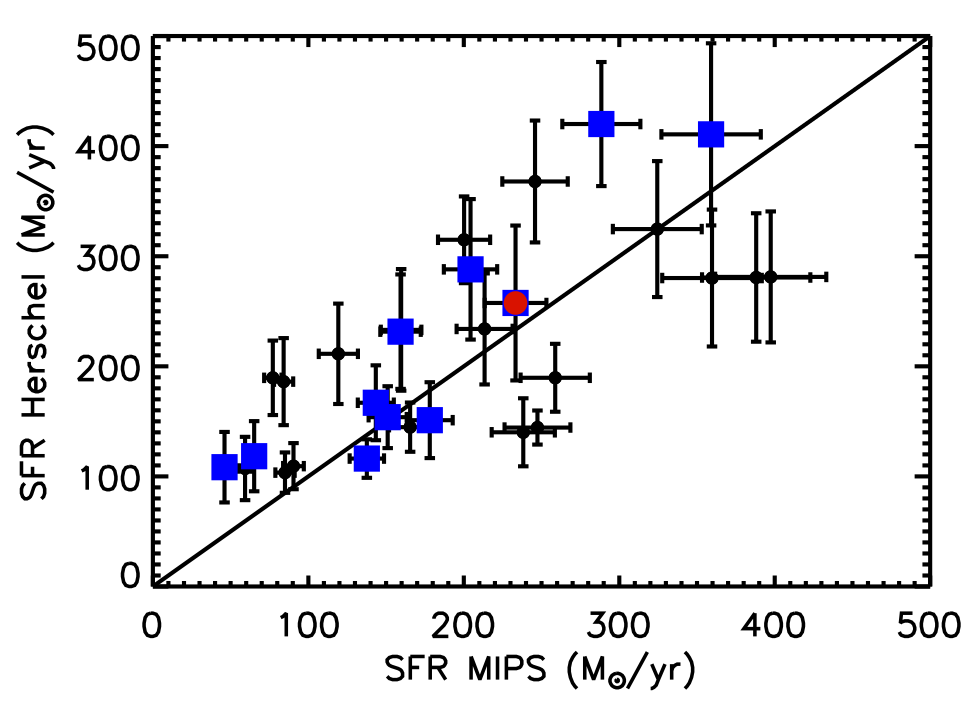
Figure 3: SFR(MIPS) vs SFR(Herschel). The red dot indicates the brightest infrared cluster galaxy (ID 16). The blue squares indicate possible contamination from neighbouring galaxies that could boost the SFRs obtained with Herschel.

5.3 Dust extinction

The mid-to-far infrared data allow us to obtain a robust estimate of the amount of extinction due to dust by directly comparing the star formation-rates obtained from the [OII] luminosity with the ones measured from the 24$\mu m$ fluxes (or full FIR SED if we have Herschel detections).

Using equation (4) of Kewley et al. (2004), we compute dust-uncorrected SFR([OII]) for a sample of 33 cluster galaxies detected both in narrow band imaging and MIPS. We find that, in order to reconcile the SFR([OII]) with the ones obtained using the 24$\mu m$ observations (corrected for the mid-IR excess problem) we require A([OII])$\sim$3 magnitudes (see Fig. 4). Similar extinction levels have been reported in the literature for galaxies at $z\sim$1.5 and with similar stellar mass (Koyama et al., 2011; Kashino, 2013). This value is a factor 3 higher than the average extinctions we obtain with the optical/NIR SED fitting analysis. The narrow range of stellar masses (median of 4$\times$10¹⁰ M_⊙) of this sample does not enable the investigation of the role of $M_{*}$ with extinction.

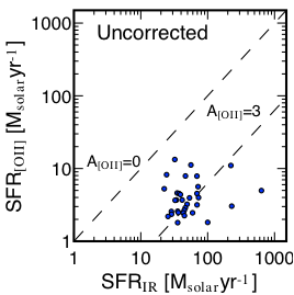
Figure 4: Comparison of the SFR([OII]) vs SFR(MIPS) for a subset of 33 galaxies detected both in narrow band imaging and MIPS. The diagonal dash lines show the amount of extinction in [OII] necessary to reconcile the two SFR diagnostics.

6 The brightest FIR cluster galaxy

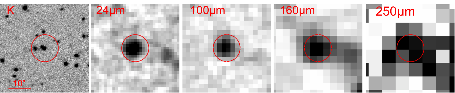
Figure 5: The brightest infrared cluster galaxy (ID 16). 40$\arcsec\times$40$\arcsec$ cutouts centered on the galaxy, from left-to-right: K-band, 24$\mu m$, 100$\mu m$, 160$\mu m$, 250$\mu m$.

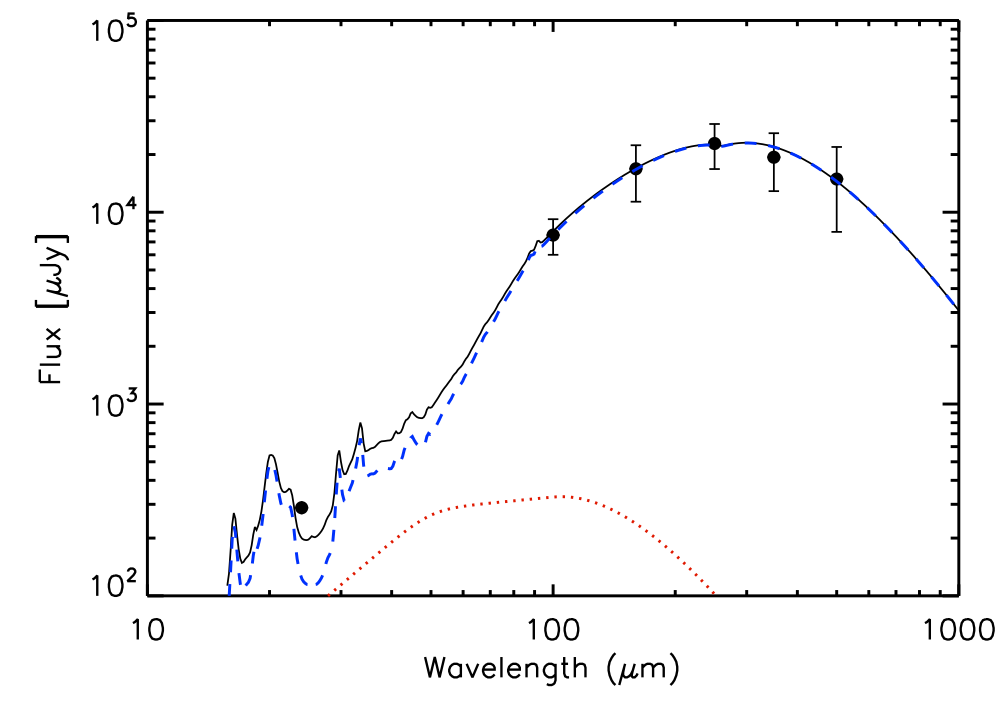
Figure 6: Spectral energy distribution (black points) of the brightest infrared cluster galaxy (ID 16) and best-fit (blue solid line). The negligible contribution from the AGN component is shown by the red dotted line.

CLG0218 hosts a relatively massive (7$\times 10^{10}$ M$\odot$) galaxy at the spectroscopic redshift 1.6238 (ID 16 in our catalogue) that dominates the cluster (i.e., $r<$ 1 Mpc) infrared emission. In previous work (e.g., Tran et al., 2010; Bassett et al., 2013) this galaxy was taken as the cluster centre hence we adopt this approach here too. Following the procedure described in §5.2 we obtain a total infrared luminosity $L_{IR,Herschel}$=3.3$\pm$1.0$\times 10^{12}L_{\odot}$, confirming that ID 16 is a ULIRG, and SFR(Herschel) = 256$\pm$70 M$\odot$/yr. We also estimate $L_{IR}$ using the method previously described based on the extrapolation from 24$\mu m$, and correct it for the mid-IR excess problem. We note that Rujopakarn et al. (2013) stress that the proposed methodology may not apply to galaxies hosting an AGN. We also note that for $z>$1 the new 24$\mu m$ indicator underestimates by a factor up to 0.5 dex the total infrared luminosity in comparison with Herschel derived luminosities (Fig. 3 of Rujopakarn et al., 2013). As expected, for ID 16 we find a lower SFR from the 24$\mu m$ flux, SFR(24$\mu m$) = 232$\pm$20 M_⊙/yr, although this is fully consistent with the Herschel derived value. This galaxy is also associated with X-ray emission detected by Chandra, therefore we investigate the contribution of the AGN component to the FIR emission, using the programme DecompIR (Mullaney et al., 2011), an SED model fitting software that attempts to separate the AGN from the host star forming (SF) galaxy. Briefly, the AGN component is an empirical model based on observations of moderate-luminosity local AGNs, whereas the 5 starburst models were developed to represent a typical range of SED types, with an extrapolation beyond 100$\mu m$ using a grey body with emissivity $\beta$ fixed to 1.5. For more details see Mullaney et al. (2011) and Seymour et al. (2012). The best-fit model obtained with DecompIR, ’SB5’, indicates that the host galaxy dominates the FIR emission, with a negligible ($\sim$4%) contribution from the AGN to the total luminosity as shown in Figure 6.

Since we have a good sampling of the FIR SED for this galaxy we are able to measure the galaxy dust temperature using a modified black body model with an emissivity index $\beta$=1.5. The fit relies only on the PACS and SPIRE data that effectively straddle the peak of the SED. We find that the cold dust component of the galaxy has a temperature $T_{dust}$=34.5$\pm$4.2 K, a value typical of high-$z$ ULIRGs (e.g., Hwang et al., 2010).

We note that, if any, the contamination from the close neighbour located at $\sim$1.5$\arcsec$ from ID 16 must be small since it is not centered with the 24$\mu m$ emission (see Fig. 5). This galaxy may belong to the cluster, with $z_{phot}$=2.0.

Since ID 16 clearly dominates the cluster SFR (the second highest star forming galaxy in the cluster has SFR=160 M_⊙/yr) we can draw a comparison with the Spiderweb galaxy (PKS1138) embedded in a proto-cluster system at $z$=2.16 (Miley et al., 2006), because less than one Gyr separates the 2 galaxies in the adopted cosmology. Unlike the Spiderweb, ID16 is not associated with significant radio emission as seen by the deep VLA catalogue of Simpson et al. (2006), nor does the AGN (X-ray) emission appear to significantly contribute to the FIR SED. The recent Herschel study of PKS1138 by Seymour et al. (2012) shows that 60% of the total infrared luminosity is due to the AGN component, and the star formation rate from the starburst corresponds to 772$\pm$83 M_⊙/yr (we scaled here the published value to the Chabrier IMF). Therefore, the core of CLG0218 appears to have a different history in comparison to PKS1138. Studies on the formation of galaxy clusters indicate that the development of the intracluster medium in the initial process of cluster virialization takes place around the brightest cluster galaxy (BCG, e.g., Voit et al., 2005). Therefore, another interesting aspect to explore is whether galaxy ID 16 could be seen as a precursor of the cluster BCG (Lapi et al., 2011). Again in PKS1138, the Spiderweb galaxy is undoubtedly the dominant galaxy of the system, with a stellar mass of the order of 10¹² M_⊙ and will most likely form the brightest cluster galaxy. In CLG0218 the scenario is different. In Papovich et al. (2011) the formation of the BCG is discussed using a sample of $K$-band selected quiescent galaxies. The authors consider that the two most massive ($\sim$2$\times$10¹¹M_⊙) spectroscopically confirmed galaxies (ID 39716 and ID 40170 in their nomenclature), separated by a projected distance of 126 kpc, will eventually merge and form the BCG with a stellar mass $>$3$\times$10¹¹ M$\odot$. Here we raise the possibility that ID 16, though at a projected distance of about 300 kpc from these two massive, quiescent galaxies, could also merge with them, contributing to the BCG as well (see Fig. 7). With the current data this is difficult to assess let alone prove, mainly because it’s not possible to accurately establish the cluster centre, however it would be interesting to follow-up on this point with kinematic studies.

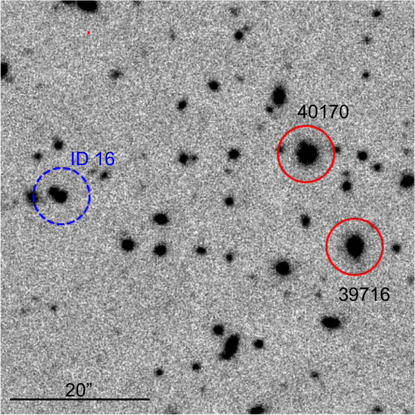
Figure 7: The cluster CLG0218 seen in the K-band (1$\arcmin\times$1$\arcmin$): ID 16 and the two most massive (quiescent) cluster galaxies. The angular scale of 20$\arcsec$ shown in the figure corresponds to a physical size of 170 kpc at redshift $z$=1.62.

7 The sSFR–$M_{*}$ relation

In this section we investigate the relation between stellar mass and star formation rate. The stellar masses were computed with the same optical/NIR SED fitting technique as described in section 4.2. We estimate a 5$\sigma$ mass completeness limit of 1.5$\times$10¹⁰ M_⊙ based on the z-band limiting magnitude (26.5 mag).

We first explore the relation between the stellar mass and SFR. In Fig. 8 we plot the specific star formation rate (sSFR=SFR/$M_{*}$) versus the stellar mass for the three galaxy samples used in our study. The deep 24$\mu m$ data allows us to reach the main sequence in this distant cluster (horizontal dash line in the figure), sSFR_MS= 1.3 Gyr^-1 obtained with the relation proposed by Elbaz et al. (2011), $sSFR_{MS}\,\,[Gyr^{-1}]=26\times t_{cosmic}^{-2.2}$. The majority of the (U)LIRGs in the CLG0218 system and environment are therefore starbursts (see Fig. 8). As shown in Table 3 and Fig. 8-right panel, we find that the median SFR increases with increasing stellar mass. This trend as well as the absolute median SFR values are very similar for the 3 galaxy samples. Given the low number statistics of the spectroscopic and [OII] emitter samples, we will use from now on the overall sample of 693 galaxies detected by MIPS.

The sSFR is essentially a measure of the star formation efficiency of galaxies, and the large scatter in the sSFR – $M_{*}$ relation is generally attributed to complex processes related with the amount of gas available or used to convert to stars (e.g. Salmi et al. 2012). A negative trend in the sSFR–$M_{*}$ relation has been reported at all redshifts (e.g. Rodighiero et al., 2010). In CLG0218 we confirm this trend, where the most massive galaxies have the lowest sSFR, that implies that more massive galaxies formed their stars earlier and more rapidly than their low mass counterparts.

The locus of the 14 star forming cluster galaxies (i.e., within 1 Mpc) forms a tight relation, described by a linear fit with slope $\alpha$ =-0.012, a mean of 2.0 Gyr^-1, and a standard deviation of 0.89 (see diagonal black solid line in Fig. 8). We compare our results on the sSFR – $M_{*}$ relation of CLG0218 with other published work. The redshift evolution of the specific SFR has been studied in a number of recent papers of which we highlight a recent compilation of data by Sargent et al. (2012). The authors find an evolutionary trend described by a power law $\propto$ (1+z)^2.8±0.1. At redshift $\sim$1.6 Fig. 1.c of Sargent et al. (2012) predicts a sSFR for galaxies with $M_{*}\sim$5$\times$10¹⁰M$\odot$ of $\sim$1.34 Gyr^-1. In CLG0218 we measure, for the same stellar mass, and using the linear fit to the 14 cluster members, a sSFR of 1.89 Gyr^-1, a value that is slightly higher than the one expected with the power law fitting function, but closer to the observational results at the same redshift from Elbaz et al. (2011). Therefore, the sSFR–$M_{*}$ relationship of the cluster CLG0218 agrees well with the relationship for the GOODS field galaxies presented in Elbaz et al. (2011).

Table 4: Star formation rates measured from the MIPS 24$\mu m$ fluxes as function of stellar mass for the 3 samples: 10 spectroscopic galaxies, [OII] emitters, photometric redshift candidates with 1.52 $<z_{phot}<$ 1.7.

Sample	Mass bin	median SFR
	(M⊙)	(M⊙/yr)
spec.	1.5–5$\times$1010	47
spec.	5–10$\times$1010	191
spec.	$\geq$1011	–
OII, $z_{phot}$	1.5–5$\times$1010	46
OII, $z_{phot}$	5–10$\times$1010	222
OII, $z_{phot}$	$\geq$1011	229
$z_{phot}$	1.5–5$\times$1010	56
$z_{phot}$	5–10$\times$1010	92
$z_{phot}$	$\geq$1011	161

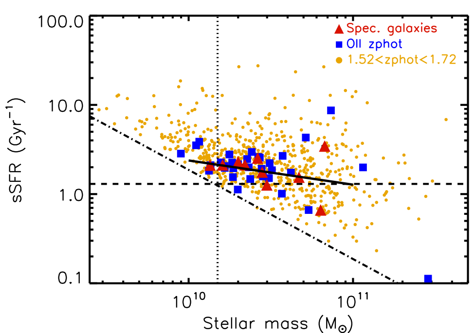
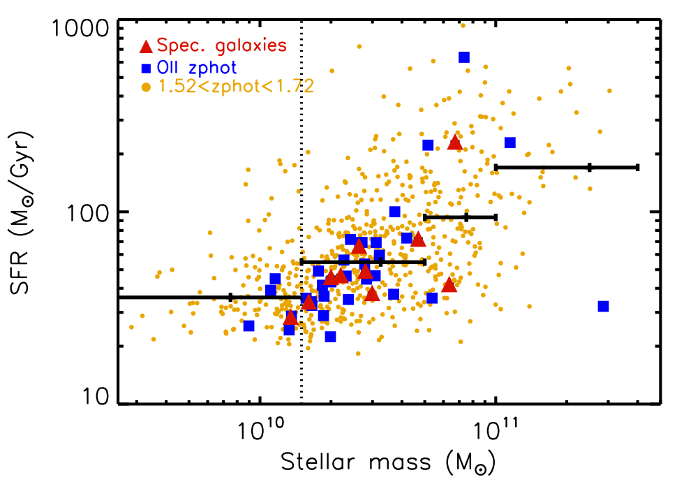
Figure 8: Left Specific star formation rate as function of stellar mass for the three samples of galaxies 1) spectroscopically galaxies at $z\sim$1.62 (red), 2) [OII] $z_{phot}$ members (blue) and MIPS emitters with 1.52$<z<$1.72 (orange). The vertical dotted line indicates our mass completeness limit; the horizontal dash line marks the main-sequence level and the diagonal dash-dot line establishes the 5-$\sigma$ sensitivity limit of our MIPS data. The solid black line is a fit to the 14 member galaxies within the cluster region ($r<$ 1 Mpc). Right Star formation rate as function of stellar mass. The median SFR of the full sample per mass bin in indicated by the horizontal black solid lines.

8 Mapping the SFR in the cluster and its environment

In this section we investigate the relation between SF, environment and galaxy stellar mass. We explore two main approaches to define and study the environment: i) fixed aperture, ii) local galaxy density. We also study the spatial distributions of the star forming and passive galaxies at 1.52$<z_{phot}<$1.72. Finally, we calculate the normalized total cluster SFR and compare it with works in the literature to gain insight on the redshift evolution of the SFR in groups and clusters.

8.1 Star formation rate vs cluster centric distance

We divide our full sample of 693 star forming galaxies in three mass bins, taking into account our mass completeness level of 1.5$\times$10¹⁰ M_⊙: 1) the low-mass bin, 1.5–5$\times$10¹⁰ M_⊙, 2) an intermediate mass category, 5–10$\times$10¹⁰ M_⊙, and 3) massive galaxies with $\geq$10¹¹ M_⊙. We then group the galaxies in 1 Mpc slices. As in Tran et al (2010) and Bassett et al (2013), we consider the cluster region to be within a radius of 1 Mpc. As suggested by Bassett et al. and Tadaki et al, the field is defined by the galaxies beyond a radius of 3 Mpc cluster centric distance. Figure 9 shows the total SFR in each bin, normalized by the bin area for the three stellar masses regimes and the combined sample. The low and intermediate mass curves follow similar trends and absolute values, with a sharp transition at a radius 1–2 Mpc where the SFR decreases by a factor $\sim$2 relative to the inner bin, and then increases at $r$ = 4–5 Mpc, stabilizing to a level of 70–90 M_⊙/yr/Mpc². The high stellar mass galaxies present a different behavior, though we are limited by small number statistics. The inner bin with 4 galaxies has a lower value of 50 M_⊙/yr/Mpc², immediately followed by a sharp decline with no galaxies in the 1–2 Mpc bin. From then on we see a marked increase in the total SFR reaching 120 M_⊙/yr/Mpc² at $r$= 3–4 Mpc, again a decrease to nearly 0, resuming to a total SFR per area at r$>$6 Mpc concordant with the lower stellar mass bins.

This figure suggests that galaxy stellar mass may play an important role in the distribution / environment of star-forming galaxies in clusters. In particular, high $M_{*}$ star forming galaxies have a low SFR contribution in the cluster region and are nearly absent in the in-falling region. In addition, we highlight the quenching action of the transition region at 1–3 Mpc, characterized by a lower SFR in star-forming galaxies of any mass bin.

The behavior of the combined stellar mass samples (black dash line in Figure 9) mirrors the trends described above. The cluster bin has a high SFR value of $\sim$300 M_⊙/yr/Mpc² which plunges down to 130 M_⊙/yr/Mpc² at 1–3 Mpc but rises to approximately the cluster value at $r$= 4 Mpc and then stabilizes to an intermediate value of $\sim$250 M_⊙/yr/Mpc². The main caveat to the interpretation of this result is that large scale substructure, ie. filaments, may bias this view at large projected distances, therefore we investigate in the next section the local galaxy density which is more insensitive to such effects.

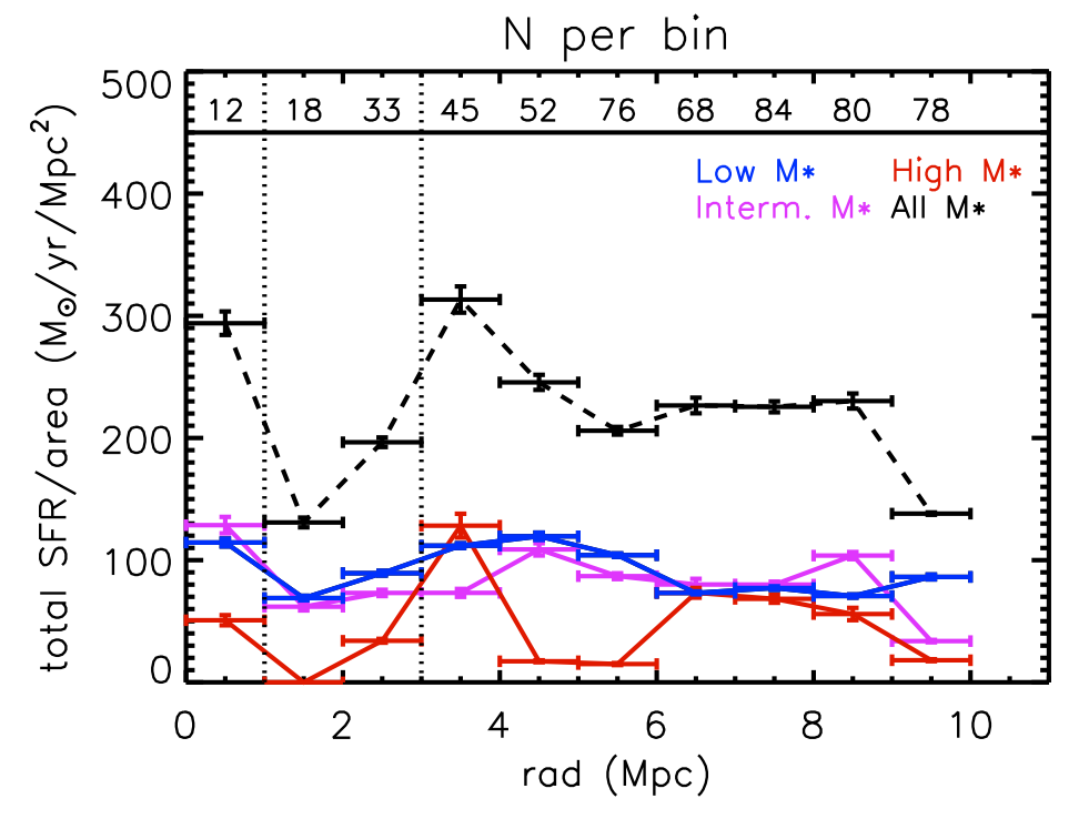
Figure 9: SFR measured in annuli of 1 Mpc width normalized by the bin area vs cluster centric distance. The SF sample is divided in 3 subsamples according to their stellar mass. The black dash line shows the results for the full (all $M_{*}$) sample, and the corresponding errors take into account the number of galaxies per bin, which are listed at the top of the plot.

8.2 Star formation rate and galaxy density

One of the most widely used techniques to study the environment in and around galaxy clusters is the use of a local density (e.g., Tanaka et al., 2006) defined as the number of galaxies within a circle of radius equal to the distance of the $n$th neighbour, normalized by the enclosed area. To be consistent with previous work we consider a local density defined with $n$=5, $\Sigma_{5}$. To compute the local density we use the combined sample of star forming and passive galaxies that lie above the mass cut $M_{*}$$>$1.5$\times$10¹⁰M_⊙.

We find no obvious trend between SFR and local density, in line with the result found by Tadaki et al. (2012) using a smaller and somewhat different sample including the [OII] emitters, and more recently Ziparo et al. (2013). However, the galaxy density maps computed with the distance to the 5th nearest neighbour for the star forming and passive galaxies independently, show two large filamentary structures several Mpc across (Fig. 10). This confirms the view that groups and clusters are found at the crossings of such matter filaments and what is generally termed the field is not simply a random distribution of galaxies.

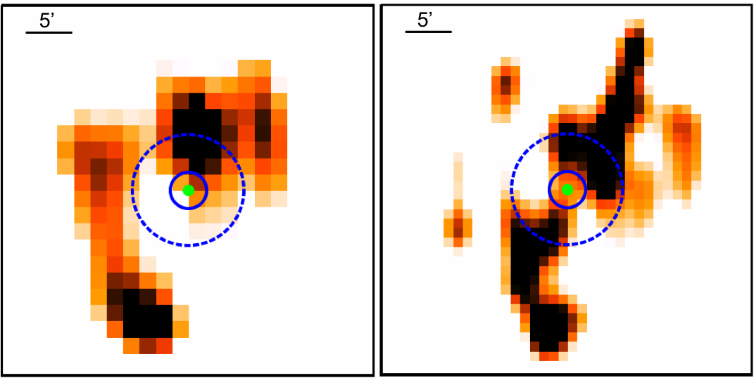
Figure 10: Gaussian smoothed density maps of the (left) passive galaxies and (right) star forming galaxies obtained with the distance to the 5th nearest neighbour. Image sizes are 40$\arcmin\times$40$\arcmin$. North is up and East is to the left. The images are centered on ID 16 (green circle), the two blue circles represent radii of 3 Mpc (dash circle) and 1 Mpc (solid). Two significant filamentary structures are seen in the upper-right and lower-left quadrants in both the passive and SF galaxy maps.

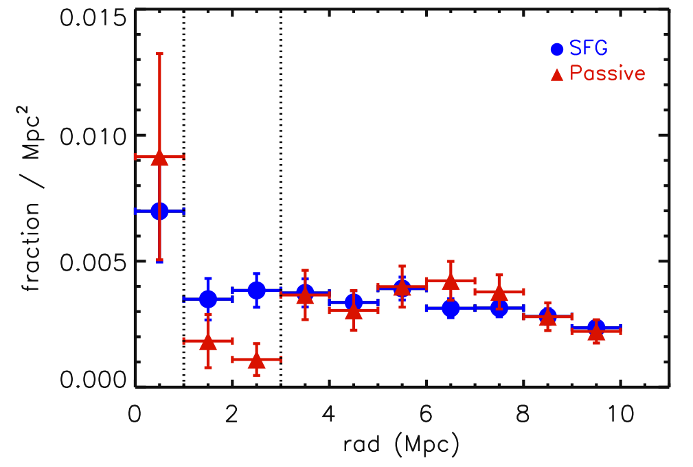
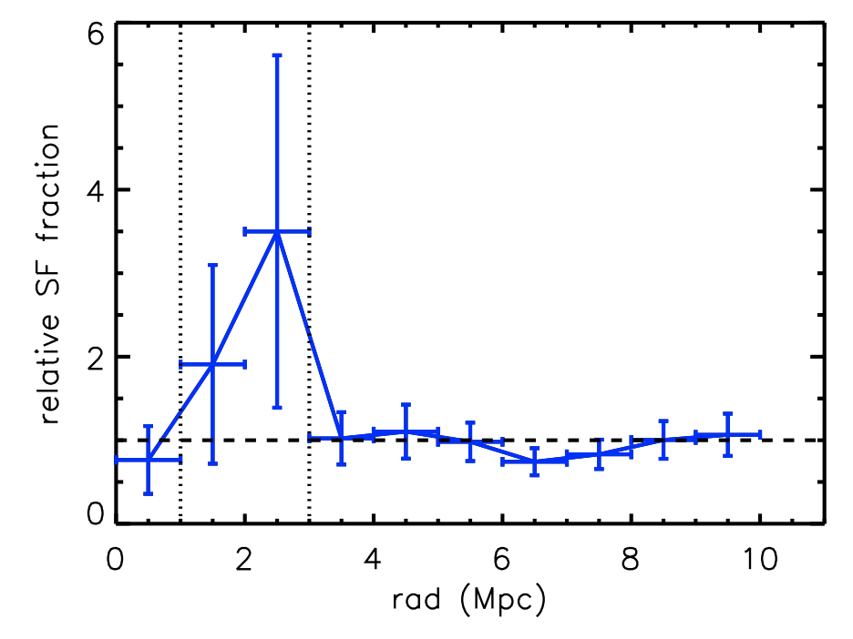
Figure 11: (Left) Fraction of star forming (blue) and quiescent (red) galaxies measured in 1 Mpc slices versus projected cluster concentric distance (Right) Ratio of the two curves displayed on the left panel.

8.3 The relative fraction of SF to passive galaxies

Besides studying the star-forming population of this cluster and its surrounding region, we also investigate the relative fraction of SF to passive galaxies in the same area. This is important because in the lower redshift Universe galaxy clusters are typically dominated by quiescent galaxies, particularly in the core (Dressler, 1980; Wilman et al., 2009). Therefore the study of the fraction of star forming galaxies covering such a large area (i.e., reaching the low galaxy density of the field) enables us to investigate a potential reversal of the SF-density relation at high-redshift.

The selection of passive galaxies was done using our optical/infrared SED catalogue. We selected galaxies with the same $z_{phot}$ range considered for the star forming galaxies, 1.52–1.72, and we excluded all sources with sSFR $>$0.01 Gyr^-1. Using these criteria we end up with a sample of 205 quiescent galaxies. By applying the mass cut $M_{*}$$>$1.5$\times$10¹⁰M_⊙ we finally have a sample of 174 quiescent galaxies, in contrast with the 547 star forming galaxies above the mass completeness level.

On the left panel of Fig. 11 we plot the relative fractions of passive and star forming galaxies (normalizing to the total number of galaxies in each sample) as a function of radius, again by binning the galaxies in 1 Mpc slices and normalized by the area covered by each bin. The errors in each bin are simply the Poisson errors. While in the cluster region ($r<$1 Mpc) and in the field area ($r>$3 Mpc) there is no statistical difference between the two samples, we find an excess of the SF fraction relative to the corresponding passive fraction in the intermediate bin, 1$<r<$3 Mpc. This behavior is quantified in the right-hand panel of Figure 11, where we plot the ratio between the 2 samples. The fraction of star forming galaxies in the transition region is $\sim$4 times larger than that of the passive galaxies, albeit the large associated errors.

Another way to compare the spatial distribution of the star forming and passive galaxies that does not rely on binned data is to compute the two-sided Kolmogorov-Smirnov (K-S) statistic of the 2 samples. This approach allows us to avoid any dependency on the bin size and consequently the statistical errors. We find that the probability of the two distributions being drawn from the same parent sample is 0.24 if we limit the test to a projected distance of 0–3 Mpc, and 0.27 when considering the full radial range. Such low probability values strengthen our previous result of significant differences between the samples of passive and star forming galaxies.

In addition, we find that the fraction of star forming galaxies is higher in the cluster than anywhere in the field (see blue line in Fig. 11, left panel). We quantify this behavior by performing a linear fit to the fraction of star forming galaxies over the radial range 1–10 Mpc. We obtain a value $f_{SF>1Mpc}$ of 0.0041, that represents the area normalized mean fraction of star forming galaxies across the transition and field regions. The central value, 0.0070$\pm$0.0050, is 1.7 times greater than the mean value, $f_{SF>1Mpc}$, however this value is hampered by the statistical errors. Hence our conclusion that the fraction of star forming galaxies is significantly enhanced in the cluster relative to the field is a tentative one (1-$\sigma$).

8.4 The mass-normalized cluster SFR

The total SFR of the system ($\Sigma$SFR) is obtained by summing up the SFR of all members above the mass limit, enclosed in a circle with 1 Mpc radius: total SFR($<$1 Mpc) = 369$\pm$31 M_⊙/yr/Mpc². We also calculate the total star formation rate within a radius of 0.5 Mpc to be able to compare our results with Tran et al. (2010), who quote a SFR ($r<$0.5 Mpc) equal to 1740 $M_{\odot}$/yr/Mpc². We find instead a lower value of the star formation in the same region: 990$\pm$121 $M_{\odot}$/yr/Mpc², using Herschel SFRs where possible. This discrepancy can be understood considering that Tran et al used the Chary & Elbaz (2001) templates that overestimate $L_{IR}$ at these redshifts. If we use SFRs from MIPS only we get a lower value, 786 $M_{\odot}$/yr/Mpc². Assuming that the SFRs derived from Herschel are the most accurate, this points to an overcorrection of the 24$\mu m$ star-formation rates when using the Rujopakarn et al method.

The mass-normalized cluster SFR is obtained by dividing $\Sigma$SFR ($<$1 Mpc) by the system gravitational mass, 5.7$\pm$1.4$\times$10¹³M_⊙ (Tanaka et al., 2010). We thus obtain, $\Sigma$SFR/M_g = 6.5$\times$10^-12 yr^-1Mpc^-2. The parameter $\Sigma$SFR/M_g has been used by several authors to quantify the evolution of the global star-formation rate in clusters with redshift. Koyama et al. (2011) confirmed previous findings on the rapid increase of the mass-normalized SFR with redshift, following the relation $\propto$ (1+$z$)⁶, though his study was based on a small sample of a dozen clusters reaching only $z\sim$ 1 and the aperture considered to compute the total SFR was 0.5 Mpc, instead of the virial radius. More recently Webb et al. (2013) performed a similar study using the Red Sequence Cluster sample with 42 clusters between 0.3$<z<$1.0 and found a similar evolutionary trend with a slope of 5.4$\pm$1.9. The authors used $r_{200}$ to compute the total SFR of the cluster and attribute the evolution to variations in the in-falling field galaxy population.

For consistency, since we consider the total cluster gravitational mass, we consider as well a radius that encompasses the total cluster mass, 1 Mpc. Comparing our value, $\Sigma$SFR/M_g =6.7$\times$10^-12 yr^-1Mpc^-2, with Figure 11 and 12 of Koyama et al. (2011), we find that CLG0218 actually falls in very good agreement with the (1+$z$)⁶ relation. Although this comparison is only qualitative, it lends support to the empirically expected significant increase in the the global star formation of CLG0218, relative to lower redshift clusters. However, our investigation of the radial distribution of the SFR presented in Fig. 9 as well as the fraction of star-forming galaxies depicted in Fig. 11 seems to be inconsistent with the hypothesis raised by Webb et al. (2013) that the in-falling galaxy population is responsible for a high level of SFR in high-$z$ clusters. Instead, the high level of SFR in the CLG0218 at $z$=1.62 is most likely due to a reversal of the SFR–density relation.

9 Conclusions

In this paper we perform a new large scale characterization of the dusty star-forming properties in and around CLG0218, a low mass galaxy cluster at $z$=1.6, using deep 24$\mu m$ MIPS and Herschel 100–500$\mu m$ imaging data covering an area of 20$\times$20 Mpc (comoving scale at the cluster redshift). Here we summarize our main findings:

1. using the 24$\mu m$ fluxes we measure luminosity based SFRs in the range 18–2500 M_⊙/yr for a sample of 693 spectroscopic and $z_{phot}$ galaxies across a radius of 10 Mpc from the cluster center;

2. for a subsample of 29 galaxies we have robust Herschel detections that allows us to assess the MIPS SFRs: although the scatter is large the overall agreement is good. While contamination from neighbouring galaxies may explain SFRs(Herschel)$>$SFRs(MIPS), it’s also possible that the methodology proposed by Rujopakarn et al. (2013) may overcorrect the SFR for high luminosity galaxies;

3. we characterize the brightest FIR cluster galaxy, ID 16, a spectroscopic member with $M_{*}$=7$\times$10¹⁰M$\odot$, SFR(Herschel)=256$\pm$70 M_⊙/yr and a dust temperature of 34.5$\pm$4.2 K. This galaxy is also taken to be the centre of the cluster. Even though there is X-ray emission associated with this galaxy we do not detect a significant AGN contribution to the FIR SED;

4. we estimate an extinction of 3 magnitudes in [OII] for the galaxies associated with CLG0218 and its environment;

5. the SFR contribution from high $M_{*}$ galaxies varies significantly with clustercentric distance and is much lower than that of the lower $M_{*}$ galaxies. High $M_{*}$ are absent in the in-falling region at 1–3 Mpc;

6. we do not find any obvious trend between the individual galaxy star-formation rates and local galaxy density parametrized by $\Sigma_{5}$;

7. we measure an enhancement by almost a factor 2 in the fraction of star-forming galaxies in the cluster (defined by an aperture with $r$= 1 Mpc) relative to the field (i.e. $r>$3 Mpc);

8. we find a significant decrease (by a factor 3.5) in the fraction of passive relative to star-forming galaxies in the in-falling region;

9. we find two large scale filamentary structures in the galaxy density maps of both the passive and the star-forming samples, showing that the galaxy distribution in the field surrounding CLG0218 is not uniform.

The enhanced fraction of star-forming galaxies at r$<$1 Mpc seen in Fig. 11 shows that SF is nearly two times larger in the higher density environment of the cluster with respect to the lower galaxy density of the surrounding field and in this sense it can be interpreted as a reversal of the SF–density relation. In addition, the similar relative fraction of SF and passive galaxies within the cluster (also seen at $r>$ 3 Mpc) is surprising and indicates this system has a young, active population of galaxies. Our study shows that the in-falling region (1–3 Mpc) is where most differences are seen in terms of dependance with stellar mass, lower SFR and deficiency of quiescent galaxies. This result is in stark contrast to the study of XMMUJ2235.3-2557, a massive galaxy cluster at $z$=1.39, in which most of the SFR seen by Herschel is at $r_{vir}$ and beyond (Santos et al., 2013). This suggests that as we move from massive distant clusters to even more distant but less massive clusters/groups, star formation migrates from the field, through the outskirts and onto to the cluster core. To better understand this effect, future studies of the star formation in high redshift clusters should include the surrounding cluster environment.

References

- Alberts et al. (2013) Alberts, S., et al. 2013, arXiv:1310.6040
- Arnouts et al. (1999) Arnouts, S.; et al., 1999, MNRAS, 310, 540
- Bai et al. (2009) Bai, L., Rieke, G. H., Rieke, M. J., Christlein, D., & Zabludoff, A. I. 2009, ApJ, 693, 1840
- Balog et al. (2013) Balog, Z., et al. 2013, arXiv:1309.6099
- Bassett et al. (2013) Bassett, R. et al. 2013, ApJ, 770, 58
- Berta et al. (2013) Berta, S., et al. 2013, A&A, 551, A100
- Brodwin et al. (2013) Brodwin, M., et al. 2013, arXiv:1310.6039
- Bruzual & Charlot (2003) Bruzual G., Charlot S., 2003, MNRAS, 344, 1000
- Calzetti (1997) Calzetti D., 1997, AIPC, 408, 403
- Calzetti et al. (2000) Calzetti D., Armus L., Bohlin R. C., Kinney A. L., Koornneef J., Storchi-Bergmann T., 2000, ApJ, 533, 682
- Chabrier (2003) Chabrier, G. 2003, PASP, 115, 763
- Chary & Elbaz (2001) Chary, R., & Elbaz, D. 2001, ApJ, 556, 562
- Dale & Helou (2002) Dale, D. A., & Helou, G. 2002, ApJ, 576, 159
- Diolaiti (2000) Diolaiti, E., Bendinelli, O., Bonaccini, D., et al. 2000, A&AS, 147, 335
- Dressler (1980) Dressler, A. 1980, ApJ, 236, 351
- Duc et al. (2002) Duc, P.-A., et al. 2002, A&A, 382, 60
- Elbaz et al. (2007) Elbaz, D., et al. 2007, A&A, 468, 33
- Elbaz et al. (2011) Elbaz, D., et al. 2011, A&A, 533, A119
- Erb et al. (2006) Erb, D. K., Shapley, A. E., Pettini, M., et al. 2006, ApJ, 644, 813
- Furusawa et al. (2008) Furusawa H., et al., 2008, ApJS, 176, 1
- Geach et al. (2006) Geach, J. E., et al. 2006, ApJ, 649, 661
- Griffin et al. (2010) Griffin, M. J., et al. 2010, A&A, 518, L3
- Haines et al. (2009) Haines, C. P., Smith, G. P., Egami, E., et al. 2009, ApJ, 704, 126
- Haines et al. (2013) Haines, C. P., et al. 2013, ApJ, 775, 126
- Hayashi et al. (2010) Hayashi, M., Kodama, T., Koyama, Y., Tanaka, I., Shimasaku, K., Okamura, S. 2010, MNRAS, 402, 1980
- Hilton et al. (2010) Hilton, M., Lloyd-Davies, E., Stanford, S. A., et al. 2010, ApJ, 718, 133
- Hwang et al. (2010) Hwang, H. S., et al. 2010, MNRAS, 409, 75
- Ilbert et al. (2006) Ilbert, O., et al. 2006, A&A, 457, 841
- Inoue et al. (2011) Inoue A. K., et al. 2011, MNRAS, 415, 2920
- Lapi et al. (2011) Lapi, A., et al. 2011, ApJ, 742, 24
- Lawrence et al. (2007) Lawrence, A., et al. 2007, MNRAS, 379, 1599
- Lutz et al. (2011) Lutz, D., et al. 2011, A&A, 532, A90
- Madau et al. (1996) Madau, P., Ferguson, H. C., Dickinson, M. E., Giavalisco, M., Steidel, C. C., Fruchter, A. 1996, MNRAS, 283, 1388
- Magnelli et al. (2011) Magnelli, B., Elbaz, D., Chary, R. R., Dickinson, M., Le Borgne, D., Frayer, D. T., Willmer, C. N. A. 2011, A&A, 528, A35
- Marcillac et al. (2008) Marcillac, D., et al. 2008, ApJ, 675, 1156
- Metcalfe et al. (2005) Metcalfe, L., Fadda, D., & Biviano, A. 2005, Space Sci. Rev., 119, 425
- Miley et al. (2006) Miley, G. K., et al. 2006, ApJ, 650, L29
- Mullaney et al. (2011) Mullaney, J. R., Alexander, D. M., Goulding, A. D., & Hickox, R. C. 2011, MNRAS, 414, 1082
- Nguyen et al. (2010) Nguyen, H. T., Schulz, B., Levenson, L., et al. 2010, A&A, 518, L5
- Noeske et al. (2007) Noeske K. G. et al., 2007, ApJL, 660, L43
- Nordon et al. (2010) Nordon, R., et al. 2010, A&A, 518, L24
- Oliver et al. (2012) Oliver, S. J., et al. 2012, MNRAS, 424, 1614
- Ott et al. (2006) Ott, S., et al. 2006, Astronomical Data Analysis Software and Systems XV, 351, 516
- Papovich et al. (2010) Papovich, C., et al. 2010, ApJ, 716, 1503
- Papovich et al. (2011) Papovich, C., et al. 2011, ApJ,
- Pierre et al. (2012) Pierre, M., Clerc, N., Maughan, B., Pacaud, F., Papovich, C., Willmer, C. N. A. 2012, A&A, 540, A4
- Pilbratt et al. (2010) Pilbratt, G. L., et al. 2010, A&A, 518, L1
- Pintos-Castro et al. (2013) Pintos-Castro, I., et al. 2013 A&A
- Poglitsch et al. (2011) Poglitsch, A., Waelkens, C., Geis, N., et al. 2010, A&A, 518, L2
- Popesso et al. (2012) Popesso, P., et al. 2012, A&A, 537, A58
- Kashino (2013) Kashino, D., et al. 2013, arXiv:1309.4774
- Kennicutt (1998) Kennicutt R. C., Jr, 1998, ARA&A, 36, 189
- Kewley et al. (2004) Kewley, L. J., Geller, M. J., & Jansen, R. A. 2004, AJ, 127, 2002
- Kodama et al. (2004) Kodama, T., Balogh, M. L., Smail, I., Bower, R. G., & Nakata, F. 2004, MNRAS, 354, 1103
- Koyama et al. (2008) Koyama, Y., et al. 2008, MNRAS, 391, 1758
- Koyama et al. (2011) Koyama, Y., Kodama, T., Nakata, F., Shimasaku, K., & Okamura, S. 2011, ApJ, 734, 66
- Lidman et al. (2008) Lidman, C., Rosati, P., Tanaka, M., et al. 2008, A&A, 489, 981
- Rieke et al. (2009) Rieke, G. H., Alonso-Herrero, A., Weiner, B. J., P rez-Gonz lez, P. G., Blaylock, M., Donley, J. L., Marcillac, D. 2009, ApJ, 692, 556
- Rodighiero et al. (2010) Rodighiero, G., et al. 2010, A&A, 518, L25
- Rujopakarn et al. (2011) Rujopakarn, W., Rieke, G. H., Eisenstein, D. J., & Juneau, S. 2011, ApJ, 726, 93
- Rujopakarn et al. (2013) Rujopakarn, W., Rieke, G. H., Weiner, B. J., P rez-Gonz lez, P., Rex, M.; Walth, G. L., Kartaltepe, J. S. 2013, ApJ, 767, 73
- Saintonge et al. (2008) Saintonge, A., Tran, K.-V. H., & Holden, B. P. 2008, ApJ, 685, L113
- Santos et al. (2013) Santos, J. S. et al. 2013, MNRAS, 433, 1287
- Sargent et al. (2012) Sargent, M. T., Béthermin, M., Daddi, E., & Elbaz, D. 2012, ApJ, 747, L31
- Seymour et al. (2012) Seymour, N., Altieri, B., De Breuck, C., et al. 2012, ApJ, 755, 146
- Simpson et al. (2006) Simpson, C., Martínez-Sansigre, A., Rawlings, S., et al. 2006, MNRAS, 372, 741
- Simpson et al. (2012) Simpson C., et al., 2012, MNRAS, 421, 3060
- Smail et al. (2008) Smail I., Sharp R., Swinbank A. M., Akiyama M., Ueda Y., Foucaud S., Almaini O., Croom S., 2008, MNRAS, 389, 407
- Smith et al. (2012) Smith, A. J., et al. 2012, MNRAS, 419, 377
- Tadaki et al. (2012) Tadaki, K.-i., et al. 2012, MNRAS, 423, 2617
- Tanaka et al. (2006) Tanaka, M., et al. 2006, MNRAS, 366, 1551
- Tanaka et al. (2010) Tanaka, M., Finoguenov, A., & Ueda, Y. 2010, ApJ, 716, L152
- Tanaka et al. (2013) Tanaka, M., et al., 2013, PASJ, 65, 17
- Tran et al. (2009) Tran, K.-V. H., et al. 2009, ApJ, 705, 809
- Tran et al. (2010) Tran, K.-V. H., et al. 2010, ApJ, 719, L126
- Voit et al. (2005) Voit, G. M. 2005, Reviews of Modern Physics, 77, 207
- Webb et al. (2013) Webb, T., et al. 2013, arXiv:1304.3335
- Wilman et al. (2009) Wilman, D. J., Oemler, A., Jr., Mulchaey, J. S., et al. 2009, ApJ, 692, 298
- Zeimann et al. (2013) Zeimann, G., et al. 2013, arXiv:1310.6037
- Ziparo et al. (2013) Ziparo, F., et al. 2013, MNRAS, 1855