Charles University in Prague
Faculty of Mathematics and Physics

DOCTORAL THESIS

Shell galaxies:

kinematical signature of shells, satellite galaxy disruption and dynamical friction

Astronomical Institute
of the Academy of Sciences of the Czech Republic

Supervisor of the doctoral thesis: RNDr. Bruno Jungwiert, Ph.D.

Study program: Physics
Specialization: Theoretical Physics, Astronomy and Astrophysics

Prague 2013

This research has made use of NASA’s Astrophysics Data System, micronised purified flavonoid fraction, and a lot of iso-butyl-propanoic-phenolic acid. Typeset in LYX, an open source document processor. For graphical presentation, we used Gnuplot, the PGPLOT (a graphics subroutine library written by Tim Pearson) and scripts and programs written by Miroslav Křížek using Python and matplotlib. Calculations and simulations have been carried out using Maple 10, Wolfram Mathematica 7.0, and own software written in programming language FORTRAN 77, Fortran 90 and Fortran 95. The software for simulation of shell galaxy formation using test particles are based on the source code of the MERGE 9 (written by Bruno Jungwiert, 2006; unpublished); kinematics of shell galaxies in the framework of the model of radial oscillations has been studied using the smove software (written by Lucie Jílková, 2011; unpublished); self-consistent simulations have been done by Kateřina Bartošková with GADGET-2 (Springel, 2005).

We acknowledge support from the following sources: grant No. 205/08/H005 by Czech Science Foundation; research plan AV0Z10030501 by Academy of Sciences of the Czech Republic; and the project SVV-267301 by Charles University in Prague. This work has been done with the support for a long-term development of the research institution RVO67985815.

I declare that I carried out this doctoral thesis independently, and only with the cited sources, literature and other professional sources.

I understand that my work relates to the rights and obligations under the Act No. 121/2000 Coll., the Copyright Act, as amended, in particular the fact that the Charles University in Prague has the right to conclude a license agreement on the use of this work as a school work pursuant to Section 60 paragraph 1 of the Copyright Act.

In Prague, 19. 8. 2013Ivana Ebrová

Title: Shell galaxies: kinematical signature of shells, satellite galaxy disruption and dynamical friction
Author: Ivana Ebrová
Department / Institute: Astronomical Institute of the Academy of Sciences of the Czech Republic
Supervisor of the doctoral thesis: RNDr. Bruno Jungwiert, Ph.D., Astronomical Institute of the Academy of Sciences of the Czech Republic

Abstract: Stellar shells observed in many giant elliptical and lenticular as well as a few spiral and dwarf galaxies presumably result from radial minor mergers of galaxies. We show that the line-of-sight velocity distribution of the shells has a quadruple-peaked shape. We found simple analytical expressions that connect the positions of the four peaks of the line profile with the mass distribution of the galaxy, namely, the circular velocity at the given shell radius and the propagation velocity of the shell. The analytical expressions were applied to a test-particle simulation of a radial minor merger, and the potential of the simulated host galaxy was successfully recovered. Shell kinematics can thus become an independent tool to determine the content and distribution of dark matter in shell galaxies up to $\sim$$100$ kpc from the center of the host galaxy. Moreover we investigate the dynamical friction and gradual disruption of the cannibalized galaxy during the shell formation in the framework of a simulation with test particles. The coupling of both effects can considerably redistribute positions and luminosities of shells. Neglecting them can lead to significant errors in attempts to date the merger in observed shell galaxies.

Keywords: galaxies: kinematics and dynamics, galaxies: interactions, galaxies: evolution, methods: analytical and numerical

1 Objectives and motivation

The most successful theory of the evolution of the Universe so far seems to be the theory of the hierarchical formation based on the assumption of the existence of cold dark matter, significantly dominating the baryonic one. In such a universe, large galaxies are formed by merging of small galaxies, protogalaxies and diffuse accretion of surrounding matter. Galactic interaction and dark matter play thus a crucial role in the life of every galaxy.

But the determination of both the dark matter content and the merger history of a galaxy is difficult. Firstly, the cold dark matter interacts only gravitationally (and possibly via the weak interaction) and thus the mapping of its distribution in galaxies is tricky. Secondly, the nature disallows us to see individual galaxies from different angles, thus our knowledge of their spatial properties is degenerate. Thirdly, it is non-trivial to determine anything about the history of a given galaxy as the whole existence of humanity presents only a snapshot in the evolution of the Universe. Yet this knowledge is important to confirm or disprove theories of the creation and evolution of the Universe, improve their accuracy and to understand how the Universe we live in actually looks.

The deal of the galactic astronomy is to try to circumvent these obstacles. One of the possibilities is to use tidal features left by the galactic interactions. They act as dynamical tracers of the potential of their host galaxies and as hints left behind by the accreted galaxies in the past. The special case is that of arc-like fine structures found in shell galaxies. Their unique kinematics carries both qualitative and quantitative information on the distribution of the dark matter, the shape of the potential of the host galaxy and its merger history. Moreover, shell galaxies have their own mysteries that call for an explanation.

?figurename? 1: Shell galaxy M89.

Some shells need to be discovered using deep photometry, e.g., Duc et al. (2011), whereas others can be today captured using amateur technology. The photography of galaxy M89 in Fig. 1 was taken by a member of our research group Michal Bílek using his own amateur equipment (taking 4.4 hours of exposure with an 8", f/4 Schmidt-Newton telescope equipped with a CCD at a site about 50 km from Prague). Faint structures were first identified by Malin (1979) and Xu et al. (2005) who concluded that the galaxy possibly possesses a low-luminosity active galactic nucleus. Michal’s image shows fairly well the shell at bottom left, the jet at bottom right and a less prominent shell at top right.

However all the information is hidden so deep in the structure and kinematics of shell galaxies that it is not clear that they could be practically unraveled. Certainly, a lot of effort and invention is required. In this work we focus mainly on the possibility to deduce the potential of the host galaxy using shell kinematics (Part II). We aim at creating equations and algorithms applicable to observed data. Now comes the era when the instrumental equipment begins to allow us to actually obtain such kind of data and that requires deeper theoretical understanding of the topic. Having no such data yet at hand, we apply our methods to simulated data. This method requires that the shell is formed by stars on mainly radial orbits. According to present state of knowledge, shells in one galaxy are probably bound by common origin in a radial minor merger. Reproducing their overall structure is nevertheless complicated by physical processes such as the dynamical friction and the gradual decay of the cannibalized galaxy. We deal with these phenomena in Part III.

Self-consistent simulations allow us to simulate many physical processes at once. Some of them are difficult or outright impossible to reproduce by analytical or semi-analytical methods. At the same time, the manifestation of these processes in self-consistent simulations is difficult to separate and sometimes they may even be confused with non-physical outcomes of used methods. Moreover, self-consistent simulations with high resolution necessary to analyze delicate tidal structures such as the shells are demanding on computation time. This demand is even larger if we want to explore a significant part of the parameter space.

Attempts to date a merger from observed positions of shells have been made in previous works. Recently, Canalizo et al. (2007) presented HST/ACS observations of spectacular shells in a quasar host galaxy (Fig. 3) and, by simulating the position of the outermost shell by means of restricted $N$-body simulations, attempted to put constraints on the age of the merger. They concluded that it occurred a few hundred Myr to $\sim 2$ Gyr ago, supporting a potential causal connection between the merger, the post-starburst ages in nuclear stellar populations, and the quasar. A typical delay of 1–2.5 Gyr between a merger and the onset of quasar activity is suggested by both $N$-body simulations by Springel et al. (2005) and observations by Ryan et al. (2008). It might therefore appear reassuring to find a similar time lag between the merger event and the quasar ignition in a study of an individual spectacular object. In Part III we explore the options for inclusion of the dynamical friction and the gradual decay of the cannibalized galaxy in test-particle simulations and we look at what these simulations tell us about the potential and merger history of shell galaxies.

In Appendix A, we show the conversion of units used in the thesis to SI units. List of abbreviations can be found in Appendix B. Videos mostly illustrating the formation and evolution of shell structures are part of the electronic attachment of the thesis. Their description can be found in Appendix H and the videos can be downloaded at: pc048b.fzu.cz/$\sim$ivana/shells/phd

?partname? I Introduction

2 Shell galaxies in brief

Shell galaxies, like e.g. the beautiful and renowned NGC 3923 in Fig. 2, are galaxies containing fine structures. These structures are made of stars and form open, concentric arcs that do not cross each other. The term shells has spread throughout the literature, gradually superseding the competing term ripples. According to the knowledge gained over the past more than thirty years, their origin lies in the interactions between galaxies.

?figurename? 2: NGC 3923 from Malin and Carter (1983) made from UK Shmidt IIIa-J plates. The bottom row shows more central parts of the galaxy. All images were processed (unsharp masking) to emphasize the shell structure. 10 ^′′ roughly corresponds to 1 kpc in the galaxy.

3 Observational knowledge of shell galaxies

This section is mostly based on the review of literature presented in Ebrová (2007).

3.1 Observational history

It was Halton Arp, who first noticed the shell galaxies in his Atlas of Peculiar Galaxies (Arp, 1966a) and the accompanying article Arp (1966b). He used the term “shells” to describe the structures associated with galaxy Arp 230. The Atlas contains 338 objects, divided into several subgroups. Shell galaxies are found under “concentric rings” (Arp numbers 227 to 231), but many other objects are in fact shell galaxies (Arp 92, 103, 104, 153–155, 171, 215, 223, 226 and probably others).

To date, the only (at least partial) list of shell galaxies is “A catalogue of elliptical galaxies with shells” from Malin and Carter (1983). The authors present a catalogue of 137 galaxies (with declination south of $-17\text{\textdegree}$) that exhibit shell or ripple features at large distances from the galaxy or in the outer envelope. Some further work has been done on this set of galaxies: Wilkinson et al. (1987a, b) examined these shell galaxies to find radio and infrared sources, Wilkinson et al. (1987c) carried out two-color CCD photometry of 66 Malin-Carter galaxies, Carter et al. (1988) obtained nuclear spectra for 100 of the galaxies in the catalogue. In a series of articles, Longhetti et al. (1998a, b); Rampazzo et al. (1999); Longhetti et al. (2000, 1999) (the fifth part surprisingly preceding the fourth) examined star formation history in 21 catalogued shell galaxies. Forbes et al. (1994) were searching for secondary nuclei in 29 shell galaxies. Larger samples of shell galaxies were studied for example by Schweizer (1983), Thronson et al. (1989), Forbes and Thomson (1992) or Colbert et al. (2001). Their results will be mentioned in the following chapters. Unsurprisingly, many observational studies have been carried out over decades for smaller samples or many individual shell galaxies.

3.2 Occurrence of shell galaxies

Originally (Arp, 1966b; Malin and Carter, 1983), shells were discovered basically in galaxies of E, E/S0 or S0 morphological type. Schweizer and Seitzer (1988) revealed that they can be found also in S0/Sa and Sa galaxies (NGC 3032, NGC 3619, NGC 4382, NGC 5739, and a Seyfert galaxy NGC 5548) and even one Sbc galaxy (NGC 3310) was found likely to contain a shell. In fact, Schweizer and Seitzer were against the term “shells”, supporting the term “ripples” being more descriptive and not forcing a particular geometric interpretation. NGC 2782 (Arp 215) is probably a spiral galaxy with shells which Arp misclassified as spiral arms rather than as shells. NGC 7531, NGC 3521, and NGC 4651 (Martínez-Delgado et al., 2010) are examples of some other lesser known cases of spiral galaxies with shells. The last of them, NGC 4651 and also M31 (Fardal et al., 2007, 2012) are the only spiral galaxies where a multiple shell system has been discovered. Coleman (2004) and Coleman et al. (2004) reported a shell, immediately followed by another one (Coleman and Da Costa, 2005; Coleman et al., 2005) in Fornax dwarf spheroidal galaxy and it became the only shell galaxy of this type.

The realistic estimate of the relative abundance of shell galaxies (Schweizer, 1983; Schweizer and Ford, 1985; cited in Hernquist and Quinn, 1988, and Malin and Carter, 1983) is about 10% in early-type galaxies. Malin and Carter (1983) state a surface brightness detection limit $\mu_{\mathrm{max}}=26.5$ mag$/$arcsec² in B filter. Schweizer and Seitzer (1988) quoted similar results for their sample of more than a hundred of galaxies, with the abundance of 6% for S0 and 10% for E type galaxies, but with significantly lower number among spirals (around 1%). Weil and Hernquist (1993a) state that Seitzer and Schweizer (1990) found 56% and 32% of 74 E and S0 type galaxies respectively posses ripples.

In a complete sample of 55 elliptical galaxies at distances 15–50 Mpc and luminosity cut of M${}_{\mbox{B}}$$<-20$ with detection limit $\mu_{\mathrm{max}}=27.7$ mag$/$arcsec² in V band, at least 22% of galaxies have shells, making them the most common interaction signature identified by Tal et al. (2009). Shells are also the most commonly detected feature in a sample of radio galaxies of Ramos Almeida et al. (2011) with $\mu_{\mathrm{max}}\sim 26$ mag$/$arcsec² in V filter.

On the contrary, in ATLAS^3D sample of 260 early-type galaxies Krajnović et al. (2011) found only 9 (3.5%) galaxies with shells at the limiting surface brightness $\mu_{\mathrm{max}}\sim 26$ mag$/$arcsec² in r band. Kim et al. (2012) examined a sample of 65 early types drawn from the Spitzer Survey of Stellar Structure in Galaxies (S⁴G) and identified 4 shell galaxies (6%). Their detection limit was 25.2 mag$/$arcsec² for newly obtained S⁴G data and 26.5 mag$/$arcsec² for some Spitzer archival images, both at 3.6 $\mu$m, which correspond to 26.9 and 28.2 mag$/$arcsec² in B band, respectively. But they failed to detect some previously known shells in at least three cases: NGC 2974 and NGC 5846 (Tal et al., 2009) and NGC 680 (Duc et al., 2011) – these three galaxies alone increase the percentage of shell galaxies in their sample to 11%. Atkinson et al. (2013) found shells in 6% of blue galaxies and around 14% in red galaxies. The survey concerns 1781 luminous galaxies with the redshift range $0.04<z<0.2$ and detection limit 27.7 mag$/$arcsec² in $\textrm{g}^{\prime}$ filter.

The occurrence of tidal features of any kind in galaxies is quite high: 73% in the sample of Tal et al. (2009); 53% in a sample of 126 red galaxies at a median redshift of $z=0.1$ and $\mu_{\mathrm{max}}\sim 28$ mag$/$arcsec² using B, V, and R filters (van Dokkum, 2005); 71% in the subsample of 86 color- and morphology- selected bulge-dominated early-type galaxies of the previous sample; about 24% in s sample of 474 close to edge-on early-type galaxies using the Sloan Digital Sky Survey DR7 archive with $\mu_{\mathrm{max}}\sim 26$ mag$/$arcsec² using $\mathrm{\textrm{u}^{\prime}}$, $\mathrm{\textrm{g}^{\prime}}$, $\textrm{r}^{\prime}$, $\mathrm{\textrm{i}^{\prime}}$, $\mathrm{\textrm{z}^{\prime}}$ bends (Miskolczi et al., 2011); 12–26% (according to confidence level of a feature identification) in the sample of Atkinson et al. (2013). The lower detection rate in Atkinson et al. (2013) is explained by authors by assertion that the majority of tidal features in early-type galaxies are seen at surface brightness near (or below) 28 mag$/$arcsec². Since shells are generally low surface brightness features, the abundance of shell galaxies will probably rise with deeper photometric observations.

Another important piece of information from the above mentioned studies is the environmental dependence of occurrence of shell structures. They are seen about five times more often in isolated galaxies than in galaxies in clusters. Malin and Carter (1983) explored 137 shell galaxies – 65 (47.5%) are isolated, 42 (30.9%) occur in loose groups (of these 13% have one or two close companions), only 5 (3.6%) occur in clusters or rich groups, and the remaining 25 (18%) occur in groups of two to five galaxies. Taking into account only isolated galaxies, the relative abundance of shell galaxies increases to 17%. Similar result was reached more recently by Colbert et al. (2001) – they detected shell/tidal features in nine of the 22 isolated galaxies (41%), but only one of the twelve (8%) group early-type galaxies shows evidence for shells. Reduzzi et al. (1996) presented their result that 4% of 54 pairs of galaxies (pairs are located in low-density environments) and 16% of 61 isolated early-type galaxies exhibit shells. Adams et al. (2012) found abundance of tidal features about 3% in a sample of 54 galaxy clusters ($0.04<z<0.15$) containing 3551 early-type galaxies, $\mu_{\mathrm{max}}=26.5$ mag$/$arcsec² in $\textrm{r}^{\prime}$ filter.

Schweizer and Ford (1985) have investigated an unbiased sample of 36 isolated giant ellipticals, in order to study their fine morphology. They found that 16 of them (44%) possess ripples (some of them very weak, as Schweizer and Ford note). In contrast to this, Marcum et al. (2004) did not find a single shell galaxy in their sample of nine early-type galaxies previously verified to exist in extremely isolated environments, even though, according to the prognosis, at least four shell galaxies should have been present. The probability of this (a sample of nine early-type galaxies from regions of low galaxy density with no shell) is about 1% if we assume that 40% of galaxies in low-density environments have shells.

However, the true abundance of shell galaxies can still be different from what has been summarized here. It crucially depends on which galaxies we classify as shell galaxies and on our ability to detect faint shells in otherwise innocent looking galaxies.

3.3 Appearance of the shells

Shells have been detected in various numbers, appearance and distributions. Rich systems like NGC 3923 (Fig. 2) or NGC 5982 (Sikkema et al., 2007) show about 30 shells, but it is rather an exception among shell galaxies. A large fraction of the Malin-Carter catalogue (1983) consists of galaxies with less then 4 shells. It is in fact difficult to make statements about numbers of shells in galaxies, because the detection of all of them (sometimes even the proof of their existence) is a delicate matter. Shells actually contain only a fraction of total luminosity of the host galaxy, mostly from 3 to 6% (e.g., it is 5% for the famous NGC 3923; Prieur, 1988). Shell surface brightness contrast is very low, about 0.1–0.2 mag (Dupraz and Combes, 1986). Schweizer (1986) states that on the brightness profiles of host galaxies, ripples appear as minor steps of about 1–10% in the local light distribution.

To enhance or detect shells and other fine structures in galaxies, some more or less sophisticated techniques are often used, like unsharp masking for photographic images (Malin, 1977), digital masking (Schweizer and Ford, 1985) or structure map (Pogge and Martini, 2002; based on the probabilistic image-restoration method of Richardson and Lucy; Richardson, 1972). Host galaxy subtraction was used to process the image of a shell galaxy in Fig. 3.

Shells are stellar structures that form arcs in galaxies (circular or slightly elliptical) that either lie within a specific double cone on opposite sides of the galaxy, or encircle the galaxy almost all around. In general, they tend to have sharp outer boundaries, but many of them are faint and diffuse. Prieur (1990) and Wilkinson et al. (1987c) recognized three different morphological categories of shell galaxies.

?figurename? 3: Top: Very deep ACS/WFC image (total integration time of 11432 s) of a formerly unknown shell galaxy, the host galaxy of the quasar MC2 1635+119 (Canalizo et al., 2007; Bennert et al., 2007; the three images shown here are unpublished and were kindly provided by G. Canalizo and N. Bennert). The shell structure is already visible in this final reduced but otherwise unaltered image. The image size is 10 ^′′$\times$10 ^′′. The residual image is shown in the bottom left panel and was obtained by subtracting a model – fitted using GALFIT (Peng et al., 2002) – for the host galaxy light (bottom right) from the original data (top). Acknowledgment: NASA, STScI.

?figurename? 4: Galaxy-subtracted image of the type I shell galaxy NGC 7600 from Turnbull et al. (1999). North is up and east is to the left. The dark oval shape is an artifact of the subtraction process. The easternmost shell lies 215 ^′′ away from the galaxy center. The field of view is 9 ^′. Acknowledgment: The Isaac Newton Group of Telescopes and the Royal Astronomical Society.

• Type I (Cone) – shells are interleaved in radius. That is, the next outermost shell is usually on the opposite side of the nucleus. They are well-aligned with the major axis of the galaxy. Shell separation increases with radius. Prominent examples are NGC 3923 (Fig. 2), NGC 5982, NGC 1344 but also NGC 7600 in Fig. 4.

• Type II (Randomly distributed arcs) – shell systems that exhibit arcs which are randomly distributed all around a rather circular galaxy. A typical example of this kind is NGC 474 in Fig. 5.

• Type III (Irregular) – shell systems that have more complex structure or have too few shells to be classified.

Prieur (1990) has found all three types in approximately the same fraction.

Dupraz and Combes (1986) state that the angular distribution of the shells is strongly related to the eccentricity of the galaxy. When the elliptical is nearly E0, the structures are randomly spread around the galactic center. On the contrary, when the galaxy appears clearly flattened ($>$E3), the shell system tends to be aligned with its major axis. In this case, shells are also interleaved on both sides of the center. Their ellipticity is in general low, but neatly correlated to the eccentricity of the elliptical. Nearly E0 galaxies are surrounded by circular shells, while the ellipticity of the shells is of about 0.15 for E3–E4 galaxies.

When we define the radial range of the shell system as the ratio between the distance from the galactic center to the outermost and the innermost shells, then this range of radii, over which shells are found, is large. The value reaches over 60 for type I galaxy NGC 3923 (the innermost shell is less than 2 kpc from center and the outermost one $\sim$100 kpc; Prieur, 1988), but in most systems, a ratio of 10 or less would be more typical. The range is lower than 5 for systems where only a few shells are detected (Dupraz and Combes, 1986).

In their sample of three shell galaxies, Fort et al. (1986) found that the characteristic thicknesses of shells are of the order of 10% or less of their distance from the center of the galaxy.

Wilkinson et al. (1987c) probed 66 of the 74 galaxies in the range from 01h 40m to 13h 46m in the Malin and Carter (1983) catalogue. They found that shells commonly occur close to the nucleus. In roughly 20% of the systems these innermost shells have spiral morphology.

?figurename? 5: Galaxy-subtracted image of the type II shell galaxy NGC 474 from Turnbull et al. (1999). North is up and east is to the left. The easternmost shell is 202 ^′′ from the galaxy center. NGC 470 is located just off the frame, $\sim$300 ^′′ west. The field of view is 9 ^′. Acknowledgment: The Isaac Newton Group of Telescopes and the Royal Astronomical Society.

3.4 Colors

At the beginning of the research on shell galaxies, it was widely believed that shells are rather bluer than the underlying galaxy (Athanassoula and Bosma, 1985). But it was rather difficult to obtain relevant data for shells with only several percent of galaxy’s luminosity and the uncertainty was probably huge.

Carter et al. (1982) presented broad-band optical and near-IR photometry of NGC 1344. The color indices derived suggest that the shell comprises a stellar population, perhaps bluer than the main body of the galaxy. The first CCD photometric observations of shell galaxies were made in April 1983 at the CFHT (Canada-France-Hawaii Telescope) by Fort et al. (1986) for their three objects (NGC 2865, NGC 5018, and NGC 3923). Unlike the shells of NGC 2865 and NGC 5018 which were found bluer than the galaxy itself, the shells of NGC 923 had similar color indices to those of the galaxy. The results were obtained from the outer shells of the galaxies.

Pence (1986) got the same result for NGC 3923 and in addition for NGC 3051 as well. On the other hand, McGaugh and Bothun (1990) found both redder and slightly bluer systems of shells among their three shell galaxies (Arp 230, NGC 7010, and Arp 223 = NGC 7585). Multicolor photometry of NGC 7010 shows a color trend between the center and the galaxy periphery, red in the center and blue further out.

Recent observations, using the ever-improving observational capabilities may turn the old myth of blue shells over. Sikkema et al. (2007) wrote: “To date, observations give a confusing picture on shell colors. Examples are found of shells that are redder, similar, or bluer, than the underlying galaxy. In some cases, different authors report opposite color differences (shell minus galaxy) for the same shell. Color even seems to change along some shells; examples are NGC 2865 (Fort et al., 1986), NGC 474 (Prieur, 1990), and NGC 3656 (Balcells, 1997). Errors in shell colors are very sensitive to the correct modeling of the underlying light distribution. HST images allow for a detailed modeling of the galaxy light distribution, especially near the centers, and should provide increased accuracy in the determination of shell colors.” In their sample of central parts of six galaxies (NGC 1344, NGC 3923, NGC 5982, NGC 474, NGC 2865, and NGC 7626) they find only one shell (in NGC 474) with blue color. All other shells have similar or redder colors – what is just contrary to the results of Fort et al. in 80’s for NGC 2865 and Carter et al. (1982) for NGC 1344. Sikkema et al. attribute the red color to dust which is physically connected to the shell (see Sect. 3.5).

Forbes et al. (1995) measured shell colors of shell galaxy IC 1459 and found them to be similar to the underlying galaxy. In their study of the shell galaxies NGC 474 and NGC 7600, Turnbull et al. (1999) found inner shells redder than the outer ones. For the first shells, colors seem to follow those of the galaxy, for NGC 7600 three outermost shells are bluer than the galaxy. In Liu et al. (1999) it is said that a preliminary reduction of the shell sample shows that most of the shells have colors that are similar to the elliptical. The shell colors in the shell galaxy MC 0422-476 are scattered around the underlying galaxy value (Wilkinson et al., 2000). Pierfederici and Rampazzo (2004) inspected another sample of five galaxies with shells (NGC 474, NGC 6776, NGC 7010, NGC 7585, and IC 1575) and found the color of the shells being similar to or slightly redder than that of the host galaxy with the exception of one of the outer shells in NGC 474, the only interacting galaxy in the sample.

3.5 Gas and dust

Athanassoula and Bosma (1985) found that shells are not a good indicator of the presence of dust. Shell galaxies (64 items) of Wilkinson et al. (1987b) have rather higher dust contain than normal elliptical. Sikkema et al. (2007) detected central dust features out of dynamical equilibrium in all of their six shell galaxies. Using HST archival data, about half of all elliptical galaxies exhibit visible dust features (Lauer et al. 2005: 47% of 177 in field galaxies). On the other hand, Colbert et al. (2001) found evidence for dust features in approximately 75% of both the isolated and group galaxies (17 of 22 and 9 of 12, respectively). But in their sample also all of the galaxies that display shell/tidal features contain dust. Also Rampazzo et al. (2007) found all of their three shell galaxies to show evidence of dust features in their center.

Moreover, Sikkema et al. (2007) discovered that the shells contain more dust per unit stellar mass than the main body of the galaxy. This could explain redder color of shells which is observed in many cases (Sect. 3.4). Observational evidence for significant amounts of dust residing in a shell was also found in NGC 5128 (Stickel et al., 2004).

In general, both the ionized and neutral gas contents of shell galaxies are thus comparable to those of normal early-type galaxies (Dupraz and Combes, 1986) or rather higher (Wilkinson et al., 1987b). However, arcs of H I have been discovered (Schiminovich et al., 1994, 1995) lying parallel to but outside of the outer stellar arcs in a few shell systems (Cen A = NGC 5128 and NGC 2865). In Centaurus A, gas has the same arc-like curvature but is displaced 1 ^′ ($\sim 1$ kpc) to the outside of the stellar shells. A similar discovery has been made by Balcells et al. (2001) in NGC 3656. The shell, at 9 kpc from the center, has traces of H I with velocities bracketing the stellar velocities, providing evidence for a dynamical association of H I and stars at the shell. Petric et al. (1997) found an off-centered H I ring in NGC 1210. A short report about H I in shell galaxies has been done by (Schiminovich et al., 1997).

Charmandaris et al. (2000) reveal the presence of dense molecular gas in the shells of NGC 5128 (Cen A). Cen A, the closest active galaxy, is a giant elliptical with jets and strong radio lobes on both sides of a prominent dust lane which is aligned with the minor axis of the galaxy (van Gorkom et al., 1990; Clarke et al., 1992; Hesser et al., 1984). A significant amount of gas and dust is situated predominantly in an equatorial disk where vigorous star formation is occurring (Dufour et al., 1979). Charmandaris et al. detected CO emission from two of the fully mapped optical shells with associated H I emission, indicating the presence of $4.3\times 10^{7}$ M_⊙ of H${}_{\text{2}}$, assuming the standard CO to H${}_{\text{2}}$ conversion ratio.

About $5\times 10^{8}$ M_⊙ of molecular gas is located in the inner 2 ^′ ($\sim 13$ kpc) of the NGC 1316 (Fornax A) and is mainly associated with the dust patches along the minor axis (Horellou et al., 2001). In addition, the four H I detections in the outer regions are all far outside the main body of NGC 1316 and lie at or close to the edge of the faint optical shells and X-ray emission of NGC 1316. The location and velocity structure of the H I are reminiscent of other shell galaxies such as Cen A.

Around $8\times 10^{7}$ M_⊙ of neutral hydrogen, and some $10^{9}$ M_⊙ of molecular hydrogen have been previously found in NGC 3656 by Balcells and Sancisi (1996). Roughly 10% of the total gas content, one third of the neutral hydrogen, lies in an extension to the south, what is also similar to Cen A. NGC 3656 also contains a prominent central dust line (Leeuw et al., 2007).

These galaxies seem to form up an interesting category of shell galaxies – aside from the shells, they also contain a prominent central dust line, good amount of gas (usually both H I and CO detected), and are usually strong radio sources with jets and active nucleus. Galaxies with these features are suspected of cannibalization of a gas-rich companion. Some examples of this group are NGC 5128 (Centaurus A), NGC 1316 (Fornax A), NGC 3656, NGC 1275 (Perseus A; massive network of dust, active nucleus; Carlson et al., 1998), IC 1575 (active nucleus in the center drives the jet orthogonally to the strong central dust lane, producing the two radio lobes; Pierfederici and Rampazzo, 2004), and possibly IC 51 (Schiminovich et al., 2013), NGC 5018 (Rampazzo et al., 2007), and NGC 7070A (Rampazzo et al., 2003).

Pellegrini (1999) found that the softer X-ray component which likely comes from hot gas, is not as large as expected for a global inflow, in a galaxy of an optical luminosity as high as that of NGC 3923. Sansom et al. (2000) find that early-type galaxies with fine structure (e.g. shells) are exclusively X-ray underluminous and, therefore, deficient in hot gas.

Rampazzo et al. (2003) analyzed the warm gas kinematics in five shell galaxies. They found that stars and gas appear to be decoupled in most cases. Rampazzo et al. (2007) , Marino et al. (2009), and Trinchieri et al. (2008) investigated star formation histories and hot gas content using the NUV and FUV Galaxy Evolution Explorer (GALEX) observations (and in the latter case also X-ray ones) in a few shell galaxies.

3.6 Radio and infrared emission

Wilkinson et al. (1987a) surveyed a subset of 64 galaxies of the Malin & Carter catalogue at 20 and 6 cm with the VLA. Apart from Fornax A, only two galaxies of their set contained obvious extended radio sources. 42% of the galaxies were detected, down to a 6-cm flux density limit of about 0.6 mJy. This detection rate does not differ significantly from normal early-type galaxies. In a complete sample of 46 southern 2 Jy radio galaxies at intermediate redshifts ($0.05<z<0.7$) of Ramos Almeida et al. (2011), 35% of galaxies have shells.

A more interesting discovery was made by Wilkinson et al. (1987b). Eight of the previous sample of 64 shell galaxies plus two from Sadler (1984) sample of E and S0 galaxies were detected by IRAS. And here comes the discovery: All of these galaxies are also radio sources with 6-cm flux densities $\geq 0.6$ mJy. They noted that according to the binomial distribution, the probability of finding all 10 galaxies at both wavelengths by chance would be 0.1%. From non-shell galaxies which are detected in the IRAS survey, only 58% are radio sources. So, there is a strong radio-infrared correlation for shell galaxies. In the tree-dimensional radio-infrared-shell space, no significant correlation is seen in any two dimensions, but a correlation is apparently found if all three are taken together.

Thronson et al. (1989) investigated infrared color-color diagram of early-type galaxies. On average, shell galaxies appear to have broadband mid- and far-infrared energy distributions very similar to those of normal S0 galaxies, although many of them were classified as ellipticals.

3.7 Other features of host galaxies

From their sample of 100 shell galaxies, Carter et al. (1988) derived that about 15–20% of shell galaxies have nuclear post-starburst spectra. Ramos Almeida et al. (2011) found shells in 15 out of 33 (45%) of the non-starburst systems, but in only 1 out of 13 (8%) of the starburst systems. All their objects are powerful radio galaxies (PRGs) and quasars.

Longhetti et al. (2000) have studied star formation history in a sample of 21 shell galaxies and 30 early-type galaxies that are members of pairs, located in very low density environments. The last star formation event (which involved different percentages of mass) that happened in the nuclear region of shell galaxies is statistically old (age of the burst from 0.1 to several Gyr) with respect to the corresponding one in the sub-sample of the interacting galaxies (age of the burst $<0.1$ Gyr or ongoing). This distinction has been possible only using diagrams involving newly calibrated “blue” indices. Assuming that stellar activity is somehow related to the shell formation, shells have to be long lasting structures.

There is an obvious strong association between kinematically distinct/decoupled cores (“KDC” or “KDCs”) and shell galaxies. First example of an elliptical galaxy with a KDC was NGC 5813 (Efstathiou et al., 1982). These galaxies are characterized by a rotation curve that shows a decoupling in rotation between the outer and inner parts of the galaxy. In some spectacular cases, the core can be spinning rapidly in the opposite direction to the outer part of the galaxy (e.g. IC 1459). It was found by Forbes (1992; cited in Hau et al., 1999) that all of the nine well-established KDCs and a further four out of the six “possible KDCs” possess shells.

Some galaxies are known to contain multiple nuclei (e.g. NGC 4936, NGC 7135, MC 0632-629, MC 0632-629). Forbes et al. (1994) conducted the first systematic search for secondary nuclei in a sample of 29 known shell galaxies. They find six (20%) galaxies with a possible secondary nucleus, what they concluded to be a probable upper limit to the true fraction of secondary nuclei. In the sample of radio galaxies of Ramos Almeida et al. (2011), five galaxies have more than one nucleus while also having shells detected. That makes 20% of their shell galaxies containing the secondary nucleus. Thereof one double nucleus is uncertain (PKS 1559+02) and one galaxy has triple nucleus indicated (PKS 0117-15). On the other hand, Longhetti et al. (1999) in their sample of 21 shell galaxies found only one (ESO 240-100) to be characterized by the presence of a double nucleus.

According to Wilkinson et al. (1987c), shell galaxies have an enormous diversity of central surface brightness. In addition, Wilkinson et al. (1987a) found a wide variety of optical appearances, suggesting that shell galaxies are not a homogeneous class with uniform physical characteristics.

4 Summary of shell characteristics

1. Shells are observed in at least 10% of early-type galaxies (E and S0) and $\sim$1% of spirals.

2. Shell galaxies occur markedly most often in regions of low galaxy density.

3. The number of shells in a galaxy ranges from 1 to $\sim$30.

4. The shells contain at most a few per cent of the overall brightness of the galaxy.

5. Surface brightness contrast of the shells is very low, about 0.1–0.2 mag.

6. Shells are of stellar nature.

7. For type I shell galaxies (see in Sect. 3.3), shells are interleaved in radius and their separation increases with radius.

8. Shells appear to be aligned with the galaxy’s major axis and slightly elliptical for flattened galaxies, and randomly spread around the galactic center for nearly E0 galaxies.

9. The radial range of shells (the ratio of the radii of the outermost and the innermost shells) is typically less then 10 but can reach over 60.

10. Shells commonly occur close to the nucleus.

11. In roughly 20% of the systems, the innermost shells have spiral morphology.

12. Shells can have any color, perhaps they are rather similar to or slightly redder than the host galaxy.

13. The colors of shells are different even in the same galaxy, tend to be red in the center and bluer further out.

14. It seems that galaxies with shells also contain central dust features.

15. An increased amount of dust has been observed in shells.

16. Slightly displaced arcs of H I, with respect to the stellar shells, have been discovered in some galaxies.

17. Molecular gas associated with shells was detected in several galaxies.

18. The detection rate of radio emission of shell galaxies is similar to other early-type galaxies.

19. There is probably a strong radio-infrared correlation for galaxies which possess shells.

20. 15–20% of shell galaxies have nuclear post-starburst spectra.

21. There is a strong association between kinematically distinct/decoupled cores and shells in galaxies.

22. The shell galaxies have an enormous diversity of central surface brightness and a wide variety of optical appearances.

5 Scenarios of shells’ origin

In the eighties and nineties several theories of formation of shell galaxies were proposed. They can be divided into three categories:

• Gas dynamical theories (Sect. 5.1) – The first truly developed theories connect star formation and the formation of shells. These theories, however, seem to be contradicted by observation and now they are not usually taken into consideration.

• Weak Interaction Model (WIM, Sect. 5.2) – According to this model, shells are density waves induced in a thick disk population of dynamically cold stars by a weak interaction with another galaxy. WIM has nice explanations for many phenomena related to the shells but suffers from some deficiencies and obscurities.

• Merger model – The most widely accepted theory is based on the idea that the stars in shells come from a cannibalized galaxy. The entire Sect. 6 is devoted to this model.

For a more detailed review, see Ebrová (2007).

5.1 Gas dynamical theories

The first theory of shell formation has been proposed by Fabian et al. (1980), who suggested that shells are regions of recent star formation in a shocked galactic wind. Gas produced by the evolution of stars in an elliptical galaxy and driven out of the galaxy in a wind powered by supernovae would be heated and compressed as it passes through a shock. As the gas cools, star formation can occur. This scenario was expanded by Bertschinger (1985) and Williams and Christiansen (1985). In the Williams and Christiansen (1985) model, shells are initiated in a blast wave expelled during an active nucleus phase early in the history of the galaxy, sweeping the interstellar medium in a gas shell, in which successive bursts of star formation occur, leading to the formation of several stellar shells.

This scenario was inspired by the supposedly bluer color of the shells, but as time and the measurements have shown, shells are composed mostly of old populations of stars (see Sect. 3.4). As Williams and Christiansen mention, star formation is a subject only to local conditions and is a stochastic process. This is in conflict with the observed interleaving of shells in many shell galaxies. Further, there is the failure to detect either ionized or neutral gas associated with the shells except in a very few cases. Dupraz and Combes (1986) argued that the mechanism of star formation in such a galactic wind is not known; the galaxy should have possessed a very large amount of interstellar matter in order to produce stellar mass of a typical shell system; and the supernovae explosions might rapidly dispel the wind which would exclude that as much as 20–25 shells form around some shell galaxies.

Loewenstein et al. (1987) reconciled previous models with the last observations at that time. Only a modest outburst is demanded by the authors to cause a period of star-formation in an outward-moving disturbance from the galactic core. The newly-formed stars occupy a small volume in the orbital phase-space of the underlying galaxy. The shells were produced in the same phase-wrapping mechanism as in the merger model (Sect. 6.1) producing an interleaved shell system (point 7 in Sect. 4). The model does not exclude the merger hypothesis, since a merger can lead to a burst of star formation in the galactic core that is the precursor of the initial blast wave. The inner shells are older than the outer ones in this scenario. This could lead to the color gradient which seems to be observed in some cases (point 13 in Sect. 4) and which was not known at the time.

All these arguments are sound, but other observed aspects of shell galaxies seem to exclude the model of Loewenstein et al. anyway. Aside from the already mentioned points, Colbert et al. (2001) discovered a consistency of the colors of the isolated galaxies with and without shells and it argues against the picture in which shells are caused by asymmetric star formation. Again the failure to detect gas in shells argues against this scenario. Finally, the lack of signs of recent star formation in the shells is the most fatal reality for the model discussed here.

A rather different scenario was proposed by Umemura and Ikeuchi (1987), and was quickly forgotten for its clumsiness and only a little agreement with observations. They tentatively considered a hot supernova-driven galactic wind as a process which produces both extended multiple stellar shells and hot X-ray coronae which have been detected around a number of early-type galaxies. Few of them also have shells (NGC 1316, NGC 1395, NGC 3923, and NGC 5128). This scenario suffers from much the same diseases as the former ones. Moreover, it gives no explanation for the increasing separation of shells with radius, since the distribution of shells is variable with the lapse of time in this scenario. As previously mentioned, early-type galaxies with fine structure are X-ray underluminous, thus deficient in hot gas (Sect. 3.5). However, this theory seems to be primarily out of game because of the observed systematic interleaving of shells.

All the models mentioned above more or less fell in condemnation and oblivion before they even started to try explaining more detailed characteristics observed in shell galaxies.

5.2 Weak Interaction Model (WIM)

Thomson and Wright (1990) came up with an elegant and revolutionary model of shell formation in elliptical/lenticular galaxies which is still in the game today. According to them, shells are density waves induced in a thick disk population of dynamically cold stars by a weak interaction with another galaxy – whence the name, the Weak Interaction Model (WIM). A year later, this hypothesis was further developed and supported by new simulations of Thomson (1991).

To support their theory, the authors state that Thronson et al. (1989) pointed out that most of the elliptical galaxies with shells catalogued by Malin and Carter (1983) are classified elsewhere as S0s. As such, a significant population of dynamically cold stars moving on nearly circular orbits could be present in these systems. They also note that faint thick disks could be present in many elliptical galaxies without detection. The authors noted that a thick-disk population which makes up only a few per cent of the total mass of a galaxy is required to explain the faint features seen in most shell galaxies. But the disk must by heavy enough to produce shells which form a few per cent of the overall brightness of the galaxy (point 4 in Sect. 4). Wilkinson et al. (2000) looked for such a disk in the shell galaxy MC 0422-476 and found no sign of an exponential disk, or any thick disk additional to the short-axis tube orbits already expected within an oblate ellipsoidal potential.

The WIM has always been simulated with the parabolic encounter of the secondary galaxy, since more circular orbits would decay rapidly during a close encounter, resulting in a merger scenario, while more hyperbolic orbits would result in encounters too quick to be effective. This fact can also account for the less frequent occurrence of shell galaxies in clusters than in the field (point 2 in Sect. 4).

Required mass of the secondary is about 0.05–0.2 of the primary mass and orbital inclination 45° or less with respect to the thick disk. The total time of the shell structure’s visibility is typically around 10 Gyr in Thomson and Wright (1990). But in the simulations of Thomson (1991), the shells are visible for only about 3 Gyr.

Possibly, the age of the shell system can be deduced from its appearance and thus the presence of a suitable secondary galaxy at an appropriate distance could be checked. But e.g. around NGC 3610 no surrounding galaxies were found (Silva and Bothun, 1998).

In WIM, the host galaxy is an oblate spheroid, and shells are readily formed as spiral density waves in the thick disk which is symmetric about the plane of symmetry of the galaxy. The model also gives the correct relative frequency of two types of shell galaxies (i.e. 1:1, Sect. 3.3), since the systems appear as type II shell galaxies when viewed at inclination angles less than approximately 60° (0° is face-on). At inclination angles larger than 60°, the systems appear as type I. As we change the viewing angle, the observed ellipticity changes from E0 (for 0°) to E4 (90°), where E4 may be the true ellipticity of the galaxy, since Prieur (1990), cited in Thomson (1991), found a strong peak at this value in the type I ellipticity histogram. However, implications of this would be somewhat strange – either all elliptical galaxies are E4 type oblate spheroids seen from different angles, or shells do occur only in E4 galaxies, what would be probably in contradiction to their relatively frequent occurrence.

Prieur (1988) pointed out that the shells in NGC 3923 are much rounder than the underlying galaxy and have an ellipticity which is similar to the inferred equipotential surfaces. This idea was originally put forward by Dupraz and Combes (1986) who found such a relationship for their merger simulations (Sect. 6). The same effect can be seen in the simulations presented by Thomson (1991).

Another advantage of the WIM lies in its ability to explain the occurrence of the shells over a broad range of radii (point 9 in Sect. 4) and close to the nucleus (point 10), since shells are formed in the thick disk that is required to be already present in the galaxy.

In his study of the shell galaxy NGC 3923, Prieur (1988) discussed varying distribution of the shells – interleaved in outer region and roughly symmetric in inner parts. According to this model, in the outer region of the galaxy, the simulations show a predominantly one-armed trailing spiral density wave which, when viewed edge-on, gives rise to the interleaving of the outer shells, naturally aligned with the major axis. Inside the perigalactic radius of the path of the intruder, the tidal forces produced during the encounter induce a bi-symmetric kinematic density wave in the thick disk. Thomson has achieved an almost breathtaking agreement with the observation of radial shell distribution, except for the innermost shells that have not appeared at all in his simulations. But he believes it could be remedied by shrinking the core radius of primary galaxy.

The WIM for shells does not predict the existence of a kinematically distinct nucleus (KDC, point 21 in Sect. 4). Hau and Thomson (1994) proposed a mechanism whereby a counter-rotating core could be formed by the retrograde passage of a massive galaxy past a slowly rotating elliptical with a pre-existing rapidly rotating central disk. In their study of the shell galaxy NGC 2865, Hau et al. (1999) state that the requirement of the WIM for the nuclear disk to be primordial is in conflict with the observed absorption line indices. It is also unlikely that a passing galaxy can transfer a large amount of orbital angular momentum over a period longer than 0.5 Gyr without being captured or substantially disrupted, as NGC 2865 has an extended massive dark halo (Schiminovich et al., 1995). Thus a purely interaction induced origin for the shells and KDC in NGC 2865 is ruled out.

The observation by Pence (1986) shows that the surface brightness of shells in NGC 3923 is a “surprisingly constant” fraction ($\sim$3–5%) of the surface brightness of the underlying galaxy. The WIM produces shells with the correct surface brightness, since they are formed in a thick disk which has the same surface brightness profile as the underlying galaxy. However, further observations (Prieur, 1988; Sikkema et al., 2007) revealed more shells in NGC 3923 that defy this rule. And there are more disobedient shell galaxies: NGC 474 and NGC 7600 (Turnbull et al., 1999) and MC 0422-476 (Wilkinson et al., 2000). Similarly for NGC 2865, the WIM origin is in conflict with the existence of bright outer shells, their blue colors, and their chaotic distribution (Fort et al., 1986).

Furthermore, Carter et al. (1998) revealed a minor axis rotation of the famous NGC 3923 what suggests a prolate or triaxial potential, and challenges the requirement of an oblate potential by the WIM. They noted that it is difficult to induce minor axis rotation in an oblate potential without inducing any corresponding major axis rotation that has not been observed.

Silva and Bothun (1998) note that the spectacular morphological fine structure of the shell galaxy NGC 3610 leads to the natural conclusion that this galaxy has undergone a recent merger event. This scenario is supported by the existence of a centrally concentrated intermediate-age stellar population which is a prediction of the dissipative gas infall models. Furthermore, the central stellar structure could have been formed by this infalling gas. It seems unlikely that the structures were formed by a non-merging tidal interaction since there is no nearby galaxy.

It is interesting that nobody has ever noticed any general one-armed spiral in the outer shells of type II shell galaxies nor any bi-symmetric spiral in inner regions. Only Wilkinson et al. (1987c) probed 66 shell galaxies and found that in roughly 20% of the systems these innermost shells have spiral morphology. But they did not specify which galaxies they were nor what spiral morphology has been found. Thomson (1991) explains: “The broken appearance of the shells is actually an interference pattern formed by the leading and trailing density waves induced during the encounter”, and he adds that the faint residual one-armed leading spiral feature seen at the end of some of the simulations is probably an $m$ = 1 kinematic density wave. The relative importance of this mode for the shell forming process is not fully understood, but it does play an important role in determining the shell morphology produced by the more massive encounters.

Wilkinson et al. (2000) found many arguments for and against the WIM in their study of the shell galaxy MC 0422-476.

Longhetti et al. (1999) favor the WIM, since they derived that in shell galaxies, the age of the last star forming event ranges from 0.1 to several Gyr. If the last burst of stellar activity that affects the absorption line strength indices, correlates with the dynamical mechanism forming the shell features, these shells are long lasting phenomena. The WIM predicts such a long life for the shells, whereas for the merger model of Quinn (1984), Sect. 6, guessed a shorter lifetime due to the initial dispersion of velocities that the stars of the shell inherited. But for example, in the framework of the merger model, Dupraz and Combes (1986) happily simulated shell systems for 10 Gyr.

A consequence of the WIM is that the stars which make up the shells must be in nearly circular orbits. That is almost opposite to the conclusions of the merger model (Sect. 6). It could be thus decided from measurements of the shell velocity fields which model is favored, but this is indeed a formidable task, as the shells contain at most a few per cent of the overall brightness of the host galaxy. Some attempts have been already carried out (Balcells and Sancisi, 1996), but as far as we know, the results are inconclusive.

To conclude, the WIM has nice explanations for many phenomena related to the shells (inner shells, shell distribution, symmetry of inner shells, etc.), for which the competing merger model (Sect. 6) seeks explanations with difficulties or has none at all. On the other side, the WIM suffers from some deficiencies and obscurities (thick disk, KDC, shells brightness, etc.). Generally, it seems to lack observational confirmation of phenomena specific to the model.

?figurename? 6: Time evolution of a cloud of test particles falling into a one dimensional Plummer potential $v-x$ space (upper row), particle radial density (lower row). The $x$ axis is centered with the center of the potential and scaled so that 1 on the axis is the Plummer radius.

6 Merger model

In this section we introduce the merger origin scenario of the shell galaxies that we consider for the rest of the thesis. For a more detailed (but slightly outdated) review, see Ebrová (2007).

6.1 Phase wrapping

The idea of a connection between mergers and shells was first published by Schweizer (1980) in his study of the shell galaxy NGC 1316 (Fornax A). The presence of shells (or “ripples” as Schweizer calls them) deep within NGC 1316 and a surprising number of galaxies with ripples but no companions fosters his belief that Fornax A, too, has been shaken by a recent intruder rather than by any of the present neighbors. Schweizer imagined that the ripples represent a milder version of the strong response that occurs in the disk of a galaxy when an intruder of comparable mass free-falls through the center: A circular density wave runs outward, followed sometimes by minor waves, and give the galaxy the appearance of a ring (Lynds and Toomre, 1976; Toomre, 1978).

Quinn (1983, 1984) took up the idea of a merger origin of shells, but showed it in a slightly different spirit. When a small galaxy (secondary) enters the scope of influence of a big elliptical galaxy (primary) on a radial or close to a radial trajectory, it splits up and its stars begin to oscillate in the potential of the big galaxy which itself remains unaffected. In their turning points, the stars have the slowest speed and thus tend to spend most of the time there, they pile up and produce arc-like structures in the luminosity profile of the host galaxy. Quinn modeled the formation of shell galaxies using test-particle and restricted $N$-body codes, much as many other did later (e.g, Hernquist and Quinn, 1987b, 1988, 1989; Dupraz and Combes, 1986) and as we will do in this work as well. It should be also noted that already Lynden-Bell (1967) described something like a pig-trough dynamics in violent relaxation in stellar systems.

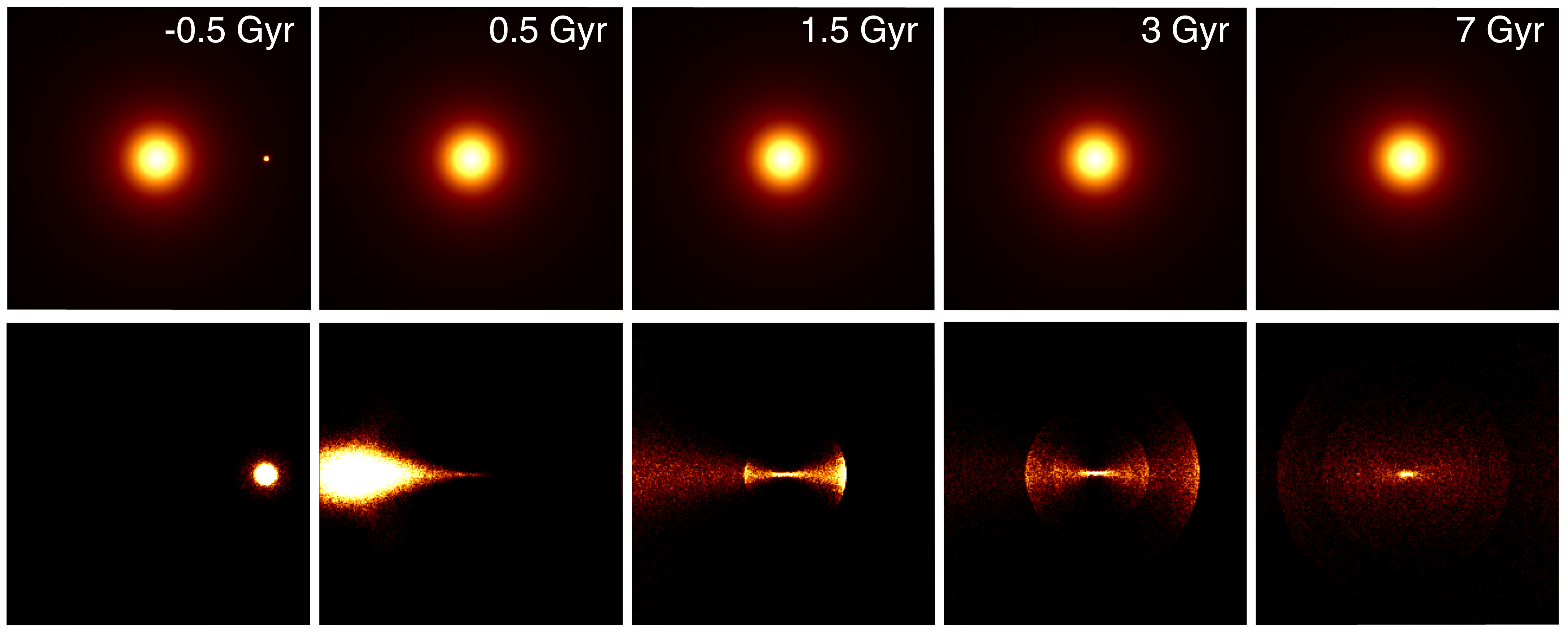
?figurename? 7: Surface brightness density from the simulation of a radial minor merger. Top row: both primary and secondary galaxy are displayed. Bottom row: only the surface density of particles originally belonging to the secondary is displayed. Panels show an area of $300\times 300$ kpc. Time-stamps mark the time since the release of the star in the center of the host galaxy. For parameters of the simulation, see Appendix H point 1.

The mechanism is illustrated on the one dimensional example in Fig. 6. The density maxima occur near the turnaround points of the particle orbits. The maximal radial position of the orbit is first reached by the most tightly bound particles, but as more distant particles stop and turn around, the density wave propagates slowly in radius to the outermost turning point set by the least bound particle. The particles in phase space form a characteristic structure, for which this mechanism of shell formation is often called “phase wrapping”.

In an idealized case, the edges in density are the caustics of the mapping of the phase density of particles into physical space (Nulsen, 1989). As a natural consequence, the shells are interleaved in radius and their separation increases with radius (point 7 in Sect. 4). Furthermore, the range of the number of shells present around ellipticals is a simple consequence of the age of the event. More shells will imply that a longer time has passed since the merger event. A more detailed explanation and some equations can be found in Sect. 9.1. The best insight on the shell formation is provided by video 1-shells.avi, which is a part of the electronic attachment. Five snapshots related to the video can be seen in Fig. 7. For the description, see Appendix H point 1.

6.2 Cannibalized galaxy

The choice of the type of the secondary galaxy initially felt on a disk galaxy. The authors were probably led to it by two aspects. Firstly, dynamically cold systems promised to be better in shell formation, since they occupy a smaller phase volume than velocity dispersion supported galaxies of comparable masses. In such a process of non-colliding stars we can assume phase volume conservation according to the Liouville’s theorem. This means that a system with an initially small phase volume keeps this property and forms sharper shells. So, the visibility of the shell system is expected to be lower for an elliptical companion than for a spiral companion of the same mass, since the velocity dispersion is greater for the elliptical. Secondly, the observations seemed to suggest that the stars in shells have the color indices of late-type galaxies (see Sect. 3.4). Later observations have shown that the shells are not that blue (see also Sect. 3.4), but even before that the simulations showed that the shell systems can be formed by a disk as well as an elliptical companion (Dupraz and Combes, 1986; Hernquist and Quinn, 1988).

Hernquist and Quinn (1988) examined among others the influence of the phase volume and velocity dispersion of a spherical companion on shell formation. As was already mentioned above, higher dispersion means higher blur of resulting shells through the increase of the phase volume (velocity dispersion is proportional to the square root of mass of the accreted companion). Another effect brought in by higher dispersion is that the material can be captured into more tightly bound orbits, so shells are produced more rapidly, since the shell production rate is indirectly proportional to the shortest period of stellar oscillations. This means that for the same potential of the primary galaxy, we can easily get different shell systems by changing some parameters of the accreted galaxy, what constituted one of several serious problems of the idea to explore the potential of the host galaxy through its shell system.

The disk-like secondary galaxy has some extra options that the spherical one lacks. By accreting differently inclined disks we can get different peculiar structures. The resulting configuration of sharp-edged features is considerably more complex and disordered than for a spherical companion. For a very flat system, there is also the possibility of forming caustics through spatial wrapping. That is to say, as the sheet of particles moves and folds in three-dimensional space, sharp edges can be formed in its two-dimensional projection onto the plane of the sky. Projection effects become critical in this context, as evidenced by the different viewing angles, see Hernquist and Quinn (1988). This effect was evident already in the simulations by Quinn (1984).

6.3 Ellipticity of the host galaxy

Dupraz and Combes (1986) tried to explain the observed characteristics of shell morphology (point 8 in Sect. 4) with the encounter of a disk galaxy with a prolate or oblate primary E-galaxy. The secondary galaxy falls into the prolate galaxy around its symmetry axis and into the oblate galaxy perpendicularly to its symmetry axis (the symmetry axis is the major axis when the E-galaxy is prolate, minor axis when oblate). The disk of the secondary galaxy is always oriented in the direction of the collision. In the prolate case, the companion stars achieve pendular motion along the major axis of the E-galaxy. The shells form consequently along this axis, alternatively on one side and the other (type I shell galaxy, see Sect. 3.3). On the contrary, in the oblate case, the shell system does not possess any symmetry, since there is no privileged major axis here. The shells appear randomly spread around the center of the E-galaxy (type II shell galaxy).

Dupraz and Combes (1986) state that a shell system is found aligned with the major axis of an elliptical galaxy, only when the E-galaxy is prolate and the impact angle is likely to be lower than 60°. A shell system is found aligned with the minor axis of an E-galaxy, only when the latter is oblate and the impact angle is lower than $\sim$30°. It is interesting to note that no such system, with the shell aligned with the minor axis, is known.

However, all this results were negated by Hernquist and Quinn (1989), who also simulated an ellipsoidal potential of the primary galaxy. Their result is that if the potential well maintains the same shape at all radii as in the simulations of Dupraz and Combes, then the shape of the dark matter halo, as well as that of the central galaxy, is responsible for aligning and confining the shells. If, on the other hand, the potential is allowed to become spherical at large radii, the shell alignment and angular extent are less sensitive to the properties of the potential at small radii. This means that two primaries, one oblate and the other prolate, can have similar projected shapes and similar outer shells if the outer isophotentials in each case become spherical. Hence the shape of the potential at large as well as small radii needs to be considered when examining the shell extent and alignment.

Even the same authors formerly tried to get some information about the potential of several chosen shell galaxies (Hernquist and Quinn, 1987b), but for those reasons and the reasons stated in Sects. 6.2 and 6.4, they were left with nothing to say but: “The shell morphology is sensitive to the shape of the primary at large and small radii as well as to the detailed structure of the companion. This would imply that it is difficult, if not impossible, to infer the form of the primary from the shell geometry alone. In this conclusion, we disagree with Dupraz and Combes (1986).”

6.4 Radial distribution of shells

The radial distribution of shells was always probably the most watched aspect of the merger model. From Sect. 6.1 we already know how easily the merger model reproduces the interleaving in radii. The shell formation is closely connected to the period of radial oscillation in the host galaxy potential, what is in any case an increasing function of radius, see Sect. 9. The shells as density waves receding from the center, composed in every moment of different stars, are the older the further from the center they are. With time, the frequency of the shells increases, thus the distances between shells decrease towards the center, what is also in agreement with observations (see Sect. 3.3).

The above-mentioned facts suggest a connection of shell distribution and the potential of the underlying galaxy. But already Quinn (1984) discovered that the radial distribution of shells derived from the potential inferred from the observed luminous matter distribution cannot agree with the observed reality. Quinn (1984) derived that the potential of the shell galaxy NGC 3923 must be less centrally condensed at radii $1<r/r_{\text{e}}<4$ (where $r_{\text{e}}$ is the half-mass radius) than the luminous matter observations predict. This discovery was reflected by Dupraz and Combes (1986); Hernquist and Quinn (1987b) as they added an extensive dark matter halo in their simulations and then they were able to better reproduce the observed shape of the shell distribution. But immediately after that, Dupraz and Combes (1987) synthesized successfully a similar radial distribution taking into account the dynamical friction instead of dark matter. Moreover, in spite of the simplicity of their model, they synthesized a wide variety of shapes for the shell distribution by varying only the two parameters: mass ratio of primary and secondary and impact parameter. It all leads to the conclusion that the shell system is not suitable to study the potential of a host galaxy.

Note that in the eighties only photometric data were considered. Merrifield and Kuijken (1998) suggested methods of measurement of the potential using shell kinematics (Sect. 7.2). The method relies on the stars, which form the shell, to be on the close-to-radial orbits and it is insensitive to the details of the merger such as the type of cannibalized galaxy and dynamic friction.

The cornerstone of the merger theory is also the huge range of radii in which the shells occur. A simple merger simulation, as of Quinn (1984) (see Sect. 6.1), is not able to produce shells simultaneously on large and small radii. The presence of shells deep within the host galaxy (and thus the presence of deeply bound stars that once were part of the secondary galaxy) was mysterious from the very beginning. But because at that time the merger model had no direct competition, it was felt more as a challenge than a flaw. However, the advent of the WIM (Sect. 5.2) that does not have any problems explaining this phenomenon, challenges the merger model more seriously.

Quinn (1984) suggested three possible explanations: First, the infall velocity of the disk may have been small and hence the disk was initially strongly bound to the elliptical. Second, the mass ratio may have been closer to unity, and hence energy could have been transferred from orbital motion to internal velocity dispersion. But as the most probable explanation he promoted the idea that the disruption process is a gradual one and that the center-of-mass motion of the disk is subject to dynamical friction.

Another effect that no one predicted was found by Heisler and White (1990). They self-consistently simulated the secondary galaxy and left the primary as a rigid potential. During the disruption event there is a substantial transfer of energy between the various parts of the satellite. Stars which lead the main body through the encounter are braked and later form the inner shell system. Stars which lag the main body are accelerated and turn into an escaping tail. This transfer is asymmetric and, for the encounters they have studied, the surviving core suffers a net loss of orbital energy which can shrink the apocenter of its orbit by a large factor. All these transfer effects increase with the mass of the satellite. It should be emphasized that this energy transfer happens only within the original secondary galaxy and no dynamical friction from the stars of the primary galaxy is accounted for in this case.

This scenario also allows the shell formation in a larger spread of radii. If the core of the cannibalized galaxy survives the merger, new generations of shells are added during each successive passage. This was predicted by Dupraz and Combes (1987) and successfully reproduced by Bartošková et al. (2011) in self-consistent simulations. Further, the combination of the loss of orbital energy in this way and the dynamical friction could bring new results, if properly modeled. This was also mentioned by Seguin and Dupraz (1996), who also simulated the formation of shell galaxies in a radial merger in a self-consistent manner, although without any dark matter halo in the primary galaxy.

6.5 Radiality of the merger

The assumption of a radial merger is the most awkward and criticized point of Quinn’s model of shell formation. In his work, Quinn (1984) has shown that if the center-of-mass motion of the infalling disk is predominantly non-radial, the merger produces confused, often overlapping shells which appear enclosing. This does not correspond to what we see in real shell galaxies.

On the other hand, A. Toomre modeled an off-axis release of a non-rotating, inclined disk into a fixed spherical force field (shown in Schweizer, 1983) and his results resemble the observed shapes. The model was similar to that of Quinn in that the disk was released as a set of test particles with identical subparabolic velocities. The shells are created via the mass transfer from the secondary galaxy flying by on a parabolic trajectory. The captured part forms a complex structure around the primary galaxy. In this case, a complete merger is not necessary to produce the shells. Hernquist and Quinn (1988) present examples of objects from the Arp atlas (Arp, 1966a) that may well have resulted from such non-merging encounters – Arp 92 (NGC 7603), 103, 104 (NGC 5216 + NGC 5218), and 171 (NGC 5718 + IC 1042) all show evidence of interactions as well as diffuse shell-like features surrounding the more luminous galaxy. Hernquist and Quinn (1988) also note that, as in the strictly planar case, the term "shell" can occasionally be a misnomer since the stars near the vicinity of a sharp edge are not necessarily distributed on a three-dimensional surface in space.

However, the requirement of a fairly radial encounter stays valid to produce type I shell galaxies (Sect. 3.3) as NGC 3923 or NGC 7600 that we have already seen in Fig. 2 and Fig. 4, respectively. A strictly radial merger of galaxies is improbable, but now cosmological $N$-body simulations tell us that satellites are preferentially accreted on very eccentric orbits (Wang et al., 2005; Benson, 2005; Khochfar and Burkert, 2006).

Dupraz and Combes (1987) considered that the shell distribution, from the parabolic encounter with dynamical friction, remains unchanged for a (small but) significant range of impact parameters. The more massive the secondary galaxy is (compared with the primary), the larger range is allowed. González-García and van Albada (2005a, b) carried out $N$-body simulations of encounters between spherical galaxies with and without a dark halo with $\sim 10^{4}$ particles. Shells are rather a byproduct of their work, but they were able to get them even for impact parameters enclosing 95% of the total mass of the primary. Even earlier, Barnes (1989) examined the evolution of a compact group of six disk galaxies in a self-consistent simulation of 65,536 particles. The result was a giant elliptical galaxy containing the shells. The shells were created during the final infall of the last galaxy into the merged body of all other galaxies. The initial distribution of the disk galaxies and their inclinations were by no means special, and Barnes did not specifically try to get the shells. This simulation may mean that during the evolution of a compact group, the shell galaxies are indeed formed in the final stage of the merger. Similarly, recently Cooper et al. (2011) found shell galaxies as a product of galaxy formation in Milky Way-mass dark halo in two from six simulated halos from the Aquarius project (Springel et al., 2008), which builds upon large-scale cosmological simulations. Furthermore, it is supported by the observed high occurrence of shells in isolated giant galaxies (Sect. 3.2).

6.6 Major mergers

Hernquist and Spergel (1992) published results of their simulation of a major merger which creates shells. Two identical galaxies with self-gravitating disks and halos merged following a close collision from a parabolic orbit. The plane of each disk initially coincides with the orbital plane. When plotted in phase space, the remnant exhibits more than 10 clearly defined phase-wraps which can be identified with shells. Shells also occur near the nucleus and appear to be aligned with the major axis of the resulting galaxies.

González-García and Balcells (2005) examined the creation of elliptical galaxies from mergers of disks. They used disk-bulge-halo or bulge-less, disk-halo models with mass ratios of the participants of 1:1, 1:2, and 1:3 and various impact parameters. As a result of those mergers, shells which could be identified in phase space occurred sometimes. They found out that the models without bulges with the mass ratio of 1:2 or 1:3 lead to more prominent shells. But these were always shell systems of type II (all-round) or type III (irregular). González-García and Balcells note the lack of shells in remnants of equal-mass mergers and on all prograde mergers. This contrasts with the shell system presented by Hernquist and Spergel (1992), a prograde merger of two equal-mass, bulge-less disks. The perfect alignment of the disk spins with the orbital angular momentum may have favored the formation of shells in their model.

González-García and van Albada (2005a, b) have also carried out simulations of encounters between spherical galaxies (see Sect. 6.5): In their first paper without a dark halo and in the second one with a dark halo (with mass ratios of 1:1, 1:2, and 1:4). The sharpness of the occurring shells was higher in models with a halo. A head-on collision for a run with mass a ratio 4:1 showed the shells even after 5 Gyr from the first encounter of the galaxy centers. But the shells showed up also in the merger with 1:2 mass ratio and a nonzero impact parameter. In any case, the shells are formed from particles of the less massive galaxy through the same phase wrapping that was established by Quinn (1984).

To summarize, shells can be formed via a merger even in the cases when the mass ratios are not as dramatic as it has been simulated in the 80s (the big mass of the secondary galaxy could influence the alignment of shells with the major axis of the host galaxy, but no one has so far explored it). It is probably not common to have shells when two disk galaxies of comparable masses merge. Hernquist and Spergel (1992) got shells in their model maybe only thanks to the very special conditions of the collision they have chosen. Furthermore, the interleaving structure and more generally the distribution of shells is not known for such cases. Some authors have guessed a major-merger origin for the shell galaxies in their observational studies (Schiminovich et al., 1995; Balcells et al., 2001; Goudfrooij et al., 2001; Serra et al., 2006).

6.7 Simulations with gas

Only a few works have been dedicated to modeling the formation of shell galaxies in the presence of gas, all of them in the framework of the minor-merger model. Weil and Hernquist (1993b) used a variant of the TREESPH code but self-gravity was strictly ignored. The primary galaxy was treated as a rigid spherically symmetric potential. They performed four runs – two radial and two non-radial; two of them were prograde with the disk inclined by 45°. Isothermal processes were assumed (T = $10^{4}$ K) except for one run where radiative cooling was allowed, and at the end 94% particles had temperature 6,000–10,000 K. Main results are that in all cases gaseous and stellar debris segregated and gas forms dense rings around the nucleus of the primary galaxy where massive star formation may occur. Furthermore the diameter of the ring depends on the impact parameter (the total angular momentum in the ring is 50% of the initial value for those particles); radial and inclined encounter forms a s-shaped ring and a counterrotating core; and about a half of all the gas particles is captured in these rings.

A completely different conclusion was reached by Kojima and Noguchi (1997). They used the sticky particle method (after collision, the radial velocity component of the particle is halved and the sign reversed) and performed four runs of simulation – radial (twice), prograde, retrograde (all with zero inclination). Both galaxies were self-gravitating systems. Star formation was modeled as a probability of a change of a gas particle to a stellar based on local gas density. They found definitely no significant segregation of gas and stars; star formation was mainly reduced because of scattering on the deep potential well of the primary (radial and retrograde runs); for slightly prograde orbit, the inner part of the secondary galaxy survives, a small stellar bar of the secondary is created which causes bar-driven gas inflow and a strong starburst. In the radial run with a less concentrated primary, a larger part of the secondary survives and the oscillating remnant destroys the shells. They state that the “poststarburst” nature of shell galaxies is due to the cessation of star formation in the disk galaxies caused by the merger (no massive star formation is caused by the encounter itself).

The model of Combes and Charmandaris (1999, 2000); Charmandaris and Combes (2000) was based on the belief in two components of galactic gas – diffuse H I gas ends in center of primary, while the small and dense gas clouds have an intermediate behavior between stars and H I. They took into account the dynamical friction and a proper treatment of the dissipation of the gas (using cloud-cloud collision code). The gaseous component was liberated first since it was less bound than stars. Then stars lose their energy due to the dynamical friction what causes some displacement of the gaseous and stellar shells. That was really observed in some shell galaxies, see Sect. 3.5.

6.8 Merger model and observations

Merger models can well explain the interleaving of shells and their increasing separation with radius (point 7 in Sect. 4) and the number of shells increases with time. The observed brightness of shells puts a lower limit to the mass of the original secondary galaxy that is usually several per cent of the primary (point 4 in Sect. 4). The question of an alignment of shells with the major axis of the host galaxy and the correlation between the type of the shell galaxy and ellipticity (point 8 in Sect. 4) remains unsettled for the merger model. The merger model has also problems explaining the large range of radii where the shells are found and their occurrence at low radii (points 9 and 10 in Sect. 4). Mergers of different secondary galaxies can explain different colors of shells and their possible difference from the color of the underlying galaxy (point 12 in Sect. 4).

A merger origin of shell systems is supported by many observations, a list of which would be lengthy. It seems that all the shell galaxies that have been so far examined in detail contain dust close to the nucleus (point 14 in Sect. 4). These dust features are often found to be out of dynamical equilibrium (Sect. 3.5), what clearly points to their external origin. Shell galaxies contain even more characteristics believed to be the results of a merger, including tidal tails, multiple nuclei or nuclear post-starburst spectra.

It seems that about 20% of shell galaxies could contain a second nucleus (Sect. 3.7) – a characteristic that one would expect in a galaxy after a merger event. Forbes et al. (1994) calculate that this could be an expected frequency due to the short lifetime of the nucleus of the secondary galaxy as opposed to the long-living shells. They note that it is also the expected frequency for the WIM origin of shell galaxies – the galaxies with the double nuclei would be those we see at the moment when the secondary galaxy just passes through the primary.

A large support for the merger theories comes from the kinematically distinct cores (KDCs). Even before it was recognized that all known galaxies with KDCs in 1992 are shell galaxies, (point 21 in Sect. 4, see also Sect. 3.7), the origin of KDCs from mergers of galaxies has been independently anticipated. Already Kormendy (1984) proposed this mechanism for the formation of counterrotating cores in elliptical galaxies and Balcells and Quinn (1990) investigated this using self-consistent numerical simulations of mergers between elliptical galaxies of unequal mass, and found that the core kinematics in the remnant depend mostly upon the orbital angular momentum at a late stage of the merger, whereas the kinematics of the outer regions is largely the original kinematics of the primary. Thus, in retrograde encounters a counter-rotating core can form. Hernquist and Barnes (1991), cited in Turnbull et al. (1999), demonstrated the formation of a counterrotating central gas disk in a merger of two gas-rich disk galaxies of equal mass. But this model is less widely accepted than the previous one. Hau and Thomson (1994) suggested a model that would comply with the WIM, but it is probably even less popular.

Enormous diversity of central surface brightness (point 22 in Sect. 4) and other characteristic show that shell galaxies are otherwise not a compact or privileged group of galaxies – so to say, the secondary cannot choose on what it falls. Still some selection effect seems to be there, because shell galaxies are much more often seen in regions with low galactic density (point 2 in Sect. 4). That can be explained with velocities in galaxy clusters being too high for one galaxy to be captured by another, or the influence of the surrounding galaxies breaks the shells structure or even prevents it from forming; or both.

Simulations show (Sect. 6.7) that in the framework of the merger model of shells’ creation, diffuse gas is introduced into the center of the host galaxy (point 20 in Sect. 4), while dense gas clouds form slightly displaced shells with respect to the stellar shells (points 16 and 17 in Sect. 4). Both are in agreement with the observations.

As the observations show, shells in galaxies are fairly common (point 1 in Sect. 4, see also Sect. 3.2). It means that in fact they occur even more frequently because from the three-dimensional shape of the shells as introduced by Quinn (1984), Sect. 6, we can easily understand that we see shells only when looking from angles close to the plane perpendicular to the line of the collision. But it is not that improbable as the shells in mergers are formed in a much larger range of impact parameters than it was originally believed (see Sect. 6.6) and interactions between galaxies are quite a common matter.

7 Measurements of gravitational potential in galaxies

Before we present our original results, we introduce the reader shortly to the topic of measuring galactic potentials, particularly in the case of elliptical and shell galaxies.

7.1 Insight into methods

The issue of the determination of the overall potential and distribution of the dark matter in galaxies is among the most prominent in galactic astrophysics. In disk galaxies, where stars and gas move on near-circular orbits, we can derive the potential (at least in the disk plane) directly up to several tens of kiloparsecs from the center of the galaxy in question. Early-type galaxies lack such kinematical beacons.

Several different methods have been used to measure the potentials and the potential gradients of elliptical galaxies, including strong gravitational lensing (e.g., Koopmans et al., 2006, 2009; Auger et al., 2010), weak gravitational lensing (e.g., Mandelbaum et al., 2008), X-ray observations of hot gas in the massive gas-rich galaxies (e.g., Fukazawa et al., 2006; Churazov et al., 2008; Das et al., 2010), rotational curves from detected disks and rings of neutral hydrogen (e.g., Weijmans et al., 2008), stellar-dynamical modeling from integrated light spectra (e.g., Thomas et al., 2011), as well using tracers such as planetary nebulae (e.g., Coccato et al., 2009), globular clusters (e.g., Norris et al., 2012) and satellite galaxies (e.g., Nierenberg et al., 2011; Deason et al., 2012).

All the methods have various limits, e.g., the redshift of the observed object, the luminosity profile, gas content, and so forth. In particular, the use of stellar dynamical modeling is plausible in the wide range of galactic masses, as far as spectroscopic data are available. However, it becomes more challenging past few optical half-light radii. Moreover, the situation is made complex by our insufficient knowledge of the anisotropy of spatial velocities. Another complementary gravitational tracers or techniques are required to derive mass profiles in outer parts of the galaxies. While comparing independent techniques for the same objects at the similar galactocentric radii, the discrepancies in the estimated circular velocity curves were revealed together with several interpretations (e.g., Churazov et al., 2010; Das et al., 2010). The compared techniques usually employ modeling the X-ray emission of the hot gas (assuming hydrostatic equilibrium) and dynamical modeling of the optical data in the massive early-type galaxies. Therefore, even for the most massive galaxies with X-ray observations at disposal, there is a need for other methods to independently constrain the gravitational potential at various radii.

7.2 Use of shells

Using the radial distribution of shells to derive the potential of the host galaxy seems tempting, but it insofar generally failed due to reasons discussed in Sect. 6.4. The question remains whether it is better to use the outer shells that are less affected by the dynamical friction and possible later generations of shells, or if we could, by careful modeling of all the relevant physical processes, reproduce the whole observed shell distribution for a suitable potential.

An alternative hypothetical use of shells to determine the dark matter content of galaxies is proposed by Sanderson et al. (2012). The increased concentration of matter and its low velocity dispersion in the shells is favorable for indirect detection of dark matter via gamma-ray emission from dark matter self-annihilation due to the Sommerfeld effect.

A slightly less exotic, though not less bold method has been proposed by Merrifield and Kuijken (1998). The method uses shells to constrain the form of the gravitational potential in the case of validity of the Quinn (1984) merger model (described in Sect. 6.1). They studied theoretically the kinematics of a stationary shell, a monoenergetic spherically symmetric system of stars oscillating on radial orbits in a spherically symmetric potential. They predicted that spectral line profiles of such a system exhibit two clear maxima, which provide a direct measure of the gradient of the gravitational potential at the shell radius.

In practice, the situation is far more complex and the shells themselves are faint structures in a bright galaxy, so the fulfillment of this program seems almost impossible. However, the authors state that they have carried out signal-to-noise ratio calculations for some of the brighter shell galaxies such as NGC 3923, and have ascertained that data of the requisite quality could be obtained with a couple of nights integration using a 4-m telescope.

Now comes the era when the instrumental equipment begins to allow us to actually obtain such kind of data and that requires deeper theoretical understanding of the topic. In Part II, we extend the work of Merrifield and Kuijken (1998) and we develop methods to better reproduce parameters of the potential of the host galaxy from measured data.

The first attempt to analyze the kinematical imprint of a shell observationally was made by Romanowsky et al. (2012), who used globular clusters as shell tracers in the early-type galaxy M87, the central galaxy in the Virgo cluster. They obtained wide-field (0–200 kpc from the center) high-precision (median velocity uncertainties: 14 km$/$s) spectroscopic data for 488 globular clusters. They found signatures of a cold stream (about 15 globular clusters at 150 kpc) and a large shell-like pattern (about 30 globular clusters between 50 and 100 kpc) and verified the presence of these features using statistical tests. These features are the first large stellar substructure with a clear kinematical detection in any type of galaxy beyond the Local Group. The stream is associated with a known stellar filament but there is no photometric shell visible in the galaxy. Typical surface brightness in the region of the shell-like pattern is $\mu_{\mathrm{V}}\sim 27$ mag$/$arcsec². Following the calculations of Merrifield and Kuijken (1998), Romanowsky et al. (2012) derived circular velocity at the shell radius $v\mathrm{{}_{c}\sim 270}$ km$/$s while X-ray data indicate $v\mathrm{{}_{c}\sim}$650–900 km$/$s in the same region. Further analysis done by the authors suggests that for such a shell to be created, the host galaxy would have to accrete a large group of dwarf galaxies or a single giant elliptical or a lenticular galaxy (about 5 times bigger than the entire Milky Way system).

Fardal et al. (2012) obtained radial velocities (median error 3 km$/$s) of 363 red giant branch stars in the region of the so-called Western Shelf in M31, the Andromeda galaxy. The Western Shelf, located about 25 kpc from the center of the galaxy, is one of several features in the stellar halo of M31. In the space of line-of-sight velocity velocity versus projected radius, the data they obtained show a wedge-like pattern. This is consistent with the previous finding of Fardal et al. (2007) who reproduced main photometric structures in the stellar halo using a simulation of an accretion of a dwarf satellite within the accurate M31 potential model. They inferred that the Western Shelf is a shell from the third orbital wrap of a tidal debris stream. Using similar simulation, Fardal et al. (2012) derived that the Western Shelf moves with phase velocity of 40 km$/$s and that the wedge pattern has a global offset -20 km$/$s with respect to the systemic velocity due to the angular momentum.

?partname? II Shell kinematics

A lot of useful information about the shell galaxies can be extracted from the kinematics of the stars forming the shell system. That it is by measuring the line-of-sight velocity distribution (LOSVD) near the edge of the shell. Now comes the era when the instrumental equipment begins to allow us to actually obtain such kind of data and that requires deeper theoretical understanding of the topic. First attempts to analyze such kind of data have been already made, see Sect. 7.2. The idea to use shell kinematics, has been proposed by Merrifield and Kuijken (1998), hereafter MK98, and we further developed it in papers Jílková et al. (2010) and Ebrová et al. (2012), Appendices LABEL:apx:clanek-lucka and LABEL:apx:clanek-huevo, respectively.

?figurename? 8: Potential of the host galaxy. The potential is modeled as a double Plummer sphere with parameters listed in Table 2.

8 Preliminary provisions

First we introduce several useful notions to aid the reader.

8.1 Host galaxy potential model

In this part of the thesis, we will often need to illustrate the shell kinematics using specific examples. For this purpose, the potential of the host galaxy is modeled as a double Plummer sphere with parameters presented in Table 1, unless specified otherwise. This model has properties consistent with observed massive early-type (and even shell) galaxies (Auger et al., 2010; Nagino and Matsushita, 2009; Fukazawa et al., 2006). The forms of the potential and density for the chosen model are shown in Figs. 8 and 9, respectively.

	Plummer radius	total mass
	kpc	M⊙
luminous component	5	$2\times 10^{11}$
dark halo	100	$1.2\times 10^{13}$

?tablename? 1: Parameters of the potential of the host galaxy used in Part II. The potential is modeled as a double Plummer sphere.

The potential of a Plummer sphere can be expressed as

$$\phi(r)=-\frac{\mathrm{G}\,M}{\sqrt{r^{2}+\varepsilon^{2}}},$$ (1)

where G is the gravitational constant, $M$ is the total mass of the galaxy, $r$ is the distance from the center of the galaxy and $\varepsilon$ is the Plummer radius. The radial density then reads

$$\rho(r)=\rho_{0}\frac{1}{(1+r^{2}/\varepsilon^{2})^{5/2}},$$ (2)

where $\rho_{0}=3M/(4\pi\varepsilon^{3})$ is the central density. The interested reader can find more on the Plummer potential in Sects. 17.2–17.4.

Let us note that such a choice of the potential of the host galaxy represents a whole class of models. For example, we can express all distances in the terms of the Plummer radius of the luminous component and all masses in the terms of the total mass of the luminous component and then choose these two parameters at will. For clarity, we nevertheless keep the specific values noted below.

?figurename? 9: Density of the host galaxy. The potential is modeled as a double Plummer sphere with parameters listed in Table 2.

8.2 Terminology

In this section, we briefly introduce terms used in next sections.

• Model of radial oscillations – through Part II, the word model is assigned to the concept described in Sect. 9 and used for modeling of shell kinematics. The model assumes that shells are made by stars on strictly radial orbits released at one moment in the center of the host galaxy. The potential of the host galaxy is chosen to represent real galaxies reasonably well. In our work, we restrict ourselves to a double Plummer sphere introduced in Sect. 8.1.

• Approximation of constant acceleration and shell velocity (Sect. 11) – it is basically the model of radial oscillations but the value of acceleration in the host galaxy as well as the value of the shell phase velocity are always constant. The approximation is assumed to be valid only in the vicinity of the shell edge. In the framework of this approximation, the position of line-of-sight velocity maxima are calculated using either of the following three methods: the approximative LOSVD (Sect. 11.2); the approximative maximal LOS velocities (Sect. 11.4); and and the method using the slope of the LOSVD intensity maxima (Sect. 11.5). Differences between these methods are summarized in Sect. 11.6.

• Higher order approximation (Sect. 12) – similarly as previous, but this time we allow the value of acceleration in the host galaxy to change linearly with galactocentric radius.

• Simulation – in this part, we only use this term when we model shell galaxies in the simulation of a radial minor merger of galaxies using test particles (Sect. 13).

8.3 Quantities

• time; usually indicates the time since the release of stars at the center of the host galaxy

• vector of Cartesian coordinates that are oriented so that the origin is at the center of the host galaxy; $x-y$ is the projected plane (“the sky”) and the $z$ direction coincides with the line of sight (LOS); $x$-axis is also the collision axis although in the model of radial oscillations it is just a virtual concept, since no collision is actually modeled

• coordinates of the projected plane

• galactocentric radius, distance from center of the galaxy; $r=\sqrt{x^{2}+y^{2}+z^{2}}$

• projected radius, the projection of $r$ into the $x-y$ plane; $R=\sqrt{x^{2}+y^{2}}$

• potential of the host galaxy; in this part, we use a spherically symmetric potential introduced in Sect. 8.1; parameters of the potential are the total mass $M_{*}$, $M_{\mathrm{DM}}$ and the scale radius $\varepsilon_{*}$, $\varepsilon_{\mathrm{DM}}$ of the luminous and dark component, respectively

• spatial density (in a spherically symmetric system)

• circular velocity; provided spherical symmetry of the galaxy, it simply denotes the quantity $\sqrt{r\phi^{\prime}(r)}$ , where $\phi^{\prime}(r)$ is the first derivative of the galactic potential with respect to the galactocentric radius $r$.

• acceleration in the host galaxy; $a_{0}$ is the constant term and $a_{1}$ is the coefficient of a linear term of the expansion of the acceleration around the shell edge

• period of radial motion at the galactocentric radius $r$ in the host galaxy potential; Eq. (4)

• serial number of a shell; shells are traditionally numbered from the outermost to the innermost ones; Sect. 9.1

• current turning point, i.e. the radius where the stars are located in their apocenters at a given moment (the moment of measurement); Eq. (3)

• phase velocity of a current turning point; Eq. (5)

• position of a star at a given time $t$ since the release of the star in the center of the host galaxy; Eqs. (6) and (7); often plain $r$ also denotes the position of stars but the meaning is clear from the context

• position of the apocenter of a star (uniquely related to the energy of the star for radial orbits); Eqs. (6) and (7)

• stellar velocity at the galactocentric radius $r$; in the model of radial oscillations the stellar velocity is always in the radial direction

• position of the edge of a shell, a function of time $r_{\mathrm{s}}(t)$; Sect. 9.2, Eq. (8)

• position of the shell edge at the moment of measurement

• phase velocity of a shell edge; approximately equal to $v_{\mathrm{TP}}$; Eq. (9)

• time when a star currently at radius $r$ will or did reach the corresponding edge of the shell; Sect. 11.1

• line-of-sight velocity; the projection of the stellar velocity into $z$ direction; $v_{\mathrm{los}}=v_{r}z/r$

• the maximal absolute value of the LOS velocity

• radius of maximal LOS velocity, radius from which comes the contribution to the LOSVD at the maximal speed $v_{\mathrm{los,max}}$; Sect. 11.3

• spot at the line of sight from which comes the contribution to the LOSVD at the maximal speed; $z_{v\mathrm{max}}=\pm\sqrt{r_{v\mathrm{max}}^{2}-R^{2}}$, Sect. 9.8

• line-of-sight velocity distribution (LOSVD); Eq. (11)

• shell-edge density distribution; Eq. (13), Sects. 9.6, 9.7, and 9.8

• discrete equivalents of $\sigma_{\mathrm{sph}}\left(r_{\mathbf{s}}\right)$; Eq. (17)

• projected surface density, the projection of spacial density into the $x-y$ plane

9 Model of radial oscillations

If we approximate the shell system with a simplified model, we can describe its evolution completely depending only on the potential of the host galaxy. The approximation lies in the numerical integration of radial trajectories of stars in a spherically symmetric potential. Stars behave as if they were released in the center of the host galaxy at the same time and their distribution of energies is continuous. Usually we demand that the distribution is continuous at least in such a range that stars with apocentra 10–30 kpc around the edge of the observed shell are present. Moreover we need that their density in this region does not go sharply to zero. In some cases, we need to know the distribution of energies explicitly. We express it in terms of the shell-edge density distribution (Sects. 9.6), which is a quantity more suitable for our situation and which can be unambiguously converted to the distribution of energies or the initial velocity distribution (Appendix C). We show that the particular choice of the function does not affect the results presented in this work (Sects. 9.7).

We call this model the model of radial oscillations, and it corresponds to the notion that the cannibalized galaxy came along a radial path and disintegrated in the center of the host galaxy. As a result the stars were released at one moment in the center and began to oscillate freely on radial orbits. This approach was first used by Quinn (1984), followed by Dupraz and Combes (1986, 1987) and Hernquist and Quinn (1987a); Hernquist and Quinn (1987b).

This model uses the exact knowledge of the chosen potential of the host galaxy, but requires it to be spherically symmetric. The potential can be given analytically or numerically and the stellar trajectories are usually integrated numerically. It differs from the real shell galaxies in several aspects but it is still the most exact analytical model that we can easily construct. We will show that in this model, the LOSVD of shells exhibits four intensity maxima and how the position of these maxima are connected with the parameters of the host galaxy potential. All the following approximations will be compared to the model of radial oscillations. Later we will show that the model agrees very well with results of test-particle simulations of the formation of the shell galaxies (Sect. 13).

9.1 Turning point positions and their velocities

In shell galaxies, the shells are traditionally numbered according to the serial number of the shell, $n$, from the outermost to the innermost (which in the model of radial oscillations for a single-generation shell system corresponds to the oldest and the youngest shell, respectively). If the cannibalized galaxy comes from the right side of the host galaxy, stars are released in the center of the host galaxy. After that, they reach their apocenters for the first time. But a shell does not form here yet, because the stars are not sufficiently phase wrapped. We call this the zeroth oscillation (the zeroth turning point) as we try to match the number of oscillations with the customary numbering scheme of the shells. We label the first shell that occurs on the right side (the same side from which the cannibalized galaxy approached) with $n=1$. Shell no. 2 appears on the left side of the host galaxy, no. 3 on the right, and so forth.

In the model of radial oscillations, the shells occur close to the radii where the stars are located in their apocenters at a given moment (the current turning point, $r_{\mathrm{TP}}$, in our notation). The shell number $n$ corresponds to the number of oscillations that the stars near the shell have completed or are about to complete. The current turning point $r_{\mathrm{TP}}$ must follow the equation

$$t=(n+1/2)T(r_{\mathrm{TP}}),$$ (3)

where $t$ is the time elapsed since stars were released in the center of the host galaxy. $T(r)$ is the period of radial motion at a galactocentric radius $r$ in the host galaxy potential $\phi(r)$:

$$T(r)=\sqrt{2}\int_{0}^{r}\left[\phi(r)-\phi(r^{\prime})\right]^{-1/2}\mathrm{d}r^{\prime}.$$ (4)

The radial period is defined as the time required for a star to travel from apocenter to pericenter and back (Binney and Tremaine, 1987).

The position of the current turning point evolves in time with a velocity given by the derivative of Eq. (3) with respect to radius

$$v_{\mathrm{TP}}(r;n)=\mathrm{d}r/\mathrm{d}t=\frac{1}{\mathrm{d}t/\mathrm{d}r}=\frac{1}{n+1/2}\left(\mathrm{d}T(r)/\mathrm{d}r\right)^{-1}.$$ (5)

We can clearly see from this relation, which was first derived by Quinn (1984), that any further turning point (turning point with higher $n$) at the same radius moves more slowly than the former one. Thus causes a gradual densification of the space distribution of the shell system with time.

Technically, the reason for this densification is that the time difference between the moments when two stars with similar energy reach their turning points is cumulative. Let $\bigtriangleup t$ be the difference in periods at two different radii $r_{\mathrm{a}}$ and $r_{\mathrm{b}}$ (with $r_{\mathrm{a}}<r_{\mathrm{b}}$, on the right). The radius where stars complete the first oscillation moves from $r_{\mathrm{a}}$ to $r_{\mathrm{b}}$ in $\bigtriangleup t$. But in the second orbit on the left, the stars from $r_{\mathrm{b}}$ will already have a lag of $\bigtriangleup t$ behind those from $r_{\mathrm{a}}$ and will just be getting a second one, so the third one (the second on the same side) reaches $r_{\mathrm{b}}$ from $r_{\mathrm{a}}$ in $3\times\bigtriangleup t$. Every $n$th completed oscillation on the right side, then moves $n$ times more slowly than the first one. The situation is similar on the left side, and the shell system is getting denser. Moreover, the turning point has an additional lag of $1/2T(r_{\mathrm{TP}})$, because the stars were released in the center of the host galaxy before their zeroth oscillation. This is the source of the factor $(n+1/2)$ in Eqs. (3) and (4).

9.2 Real shell positions and velocities

Even in the framework of the model of radial oscillations, the position and velocity of the true edge of the shell cannot be expressed in a straightforward manner. Photometrically, shells appear as a step in the luminosity profile of the galaxy with a sharp outer cut-off. This is because the stars of the cannibalized galaxy occupy a limited volume in the phase space. With time, the shape of this volume gets thinner, more elongated, and wrapped around invariant surfaces defined by the trajectories of the stars in the phase space, increasing its coincidence with these surfaces. A shell appears close to the points where the invariant surface is perpendicular to the plane of the sky (Nulsen, 1989). For the $n$th shell, this is the largest radius where stars about to complete their $n$th oscillation are currently located. This radius corresponds to the shell edge (Sect. 9.3) and it is always larger than that of the current turning point of the stars that are completing their $n$th oscillation. Thus, the shell edge consists of outward-moving stars about to complete their $n$th oscillation.

Dupraz and Combes (1986) state that the stars forming the shell move with the phase velocity of the shell. While we show that this holds only roughly, we use this approximation in Sect. 11 to derive the relation between the shell kinematics and the potential of the host galaxy.

The position of a star, $r_{\mathrm{*}}$, at a given time $t$ since the release of the star in the center of the host galaxy is given by an implicit equation for $r_{\mathrm{*}}$ and is a function of the star energy, or equivalently the position of its apocenter $r_{\mathrm{ac}}$. For stars with the integer part of $t/[2T(r_{\mathrm{ac}})]$ odd, the equation reads:

$$\begin{array}[]{rcl}t=(n+1)\sqrt{2}&\int_{0}^{r_{\mathrm{ac}}}&\left[\phi(r_{\mathrm{ac}})-\phi(r^{\prime})\right]^{-1/2}\mathrm{d}r^{\prime}-\\ -&\int_{0}^{r_{\mathrm{*}}}&\left[2(\phi(r_{\mathrm{ac}})-\phi(r^{\prime}))\right]^{-1/2}\mathrm{d}r^{\prime}.\end{array}$$ (6)

For stars that have completed an even number of half-periods (only such stars are found on the shell edge), the equation is

$$\begin{array}[]{rcl}t=n\sqrt{2}&\int_{0}^{r_{\mathrm{ac}}}&\left[\phi(r_{\mathrm{ac}})-\phi(r^{\prime})\right]^{-1/2}\mathrm{d}r^{\prime}+\\ +&\int_{0}^{r_{\mathrm{*}}}&\left[2(\phi(r_{\mathrm{ac}})-\phi(r^{\prime}))\right]^{-1/2}\mathrm{d}r^{\prime}.\end{array}$$ (7)

The first term in Eq. (7) corresponds to $n$ radial periods for the star’s energy ($n$ is maximal so that $nT(r_{\mathrm{ac}})<t$), while the other term corresponds to the time that it takes to reach radius $r_{\mathrm{*}}$ from the center of the galaxy. Even for the simplest galactic potentials, these equations are not analytically solvable and must be solved numerically.

The position of the $n$th shell $r_{\mathrm{s}}$ equals the maximal radius $r_{\mathrm{*}}$ that solves Eq. (7) for the given $n$. In symbolic notation

$$r_{\mathrm{s}}=\mathrm{max}\{r_{\mathrm{*}}(r_{\mathrm{ac}});\left\lfloor t/T(r_{\mathrm{ac}})\right\rfloor=n-1\},$$ (8)

where $r_{\mathrm{*}}(r_{\mathrm{ac}})$ is an implicit function given by Eq. (7). Simultaneously, we require $r_{\mathrm{ac}}$ to satisfy the equation $\left\lfloor t/T(r_{\mathrm{ac}})\right\rfloor=n-1$, where $\left\lfloor x\right\rfloor$ indicates the integer part of $x$, so that $\left\lfloor t/T(r_{\mathrm{ac}})\right\rfloor$ is the number of periods completed by the star since the release of the star in the center of the host galaxy. Radial period $T(r_{\mathrm{ac}})$ is defined by Eq. (4) and $n$ is the serial number of the shell for which we want to find the edge radius $r_{\mathrm{s}}$.

Such a radius is actually identical to the step in projected surface density that corresponds to the shell edge (Sect. 9.3). For a shell with nonzero phase velocity the shell edge is always further from the center than the current turning point, $r_{\mathrm{TP}}<r_{\mathrm{s}}$. On the other hand, the apocenter $r_{\mathrm{ac}}$ of a star currently located at the shell edge is obviously further from the center than the current shell edge position.

The shell velocity $v_{\mathrm{s}}$ is obtained from the numerical derivative of a set of values of $r_{\mathrm{s}}$ for several close values of $t$

$$v_{\mathrm{s}}=\mathrm{d}r_{\mathrm{s}}/\mathrm{d}t.$$ (9)

The stellar velocity at the shell edge, $v_{r}(r_{\mathrm{s}})$, is obtained by inserting $r_{\mathrm{s}}$ with its corresponding $r_{\mathrm{ac}}$ into:

$$v_{r}(r_{\mathrm{*}})=\pm\sqrt{2[\phi(r_{\mathrm{ac}})-\phi(r_{\mathrm{*}})]}.$$ (10)

For the stars following Eq. (7), the velocity will be positive; for the rest, it will be negative. The positive velocity means that the stars are moving outward. The edge of a shell is exclusively made up of stars with positive velocities. Recall that the star moves along radial trajectories.

It is clear that $v_{r}(r_{\mathrm{s}})\leq v_{\mathrm{s}}$. Actually, $v_{r}(r_{\mathrm{s}})$ is lower than the phase velocity of the shell (Table 2) but the difference between the values of these velocities is small. At the same time, the position of the shell for a given time is not far from the current turning point, and their separation changes slowly in galactic potentials. Thus, the velocity of the turning points given in Eq. (5) is a good approximation for the shell velocity (Fig. 14). Eq. (5) is not generally solvable analytically either, but the numerical calculation of $v_{\mathrm{TP}}$ is much easier than determining the true shell velocity $v_{\mathrm{s}}$. The procedure to calculate $v_{\mathrm{s}}$ is described in this section.

?figurename? 10: Projected surface density of shells in the host galaxy, with potential introduced in Sect. 8.1, 2.2 Gyr after the release of the stars in the center. The scale bar is logarithmic in arbitrary units.

9.3 Appearance of the shells

The model of radial oscillations is primarily used for calculating the positions of LOSVD maxima. Nevertheless, we can also use it to derive the spatial and projected surface density of the stars that form the shell ($\rho(r)$ and $\Sigma_{\mathrm{los}}(R)$, respectively) and the shape of the LOSVD itself. We do not aim to produce these quantities with such a precision that would be required for comparison with observation within this model. But we can still have a look at them to obtain qualitative insight, although their exact shape is not important for our work.

To do that, it is not sufficient to know the kinematics as described in Sect. 9.2 but we need to add an assumption about the radial dependence of the shell-edge density distribution $\sigma_{\mathrm{sph}}\left(r_{\mathbf{s}}\right)$. We chose this to correspond to a constant number of stars at the edge of the shell; for more details, see Sects. 9.6, 9.7, and 9.8. Furthermore we assume that the density of stars on the shells has uniform angular distribution. In most cases, we follow the shell kinematics only between $0.9r_{\mathrm{s}}-r_{\mathrm{s}}$ and thus an opening angle of at least $51.7\text{\textdegree}$ is sufficient.

Fig. 10 shows the projected surface density of the five outermost shells at 2.2 Gyr after the release of the stars in the center of the host galaxy (for parameters of the potential, see Sect. 8.1). Projected surface density of the host galaxy itself is not displayed. The opening angle of the shells is chosen to be the full $180\text{\textdegree}$. Shells with an odd serial number are to the right, those with an even number to the left, corresponding to the cannibalized galaxy flying in from the right hand side of the host galaxy. The whole picture is analogical to the results of the N-particle simulation analyzed in Sect. 13.2.

In practice, such a projected surface density depends only on the projected radius $R$ and it is shown also in Fig. 11. Jumps in the density do indeed correspond to the radius $r_{\mathrm{s}}$ in the sense in which it is introduced in Sect. 9.2, Eq. (8).

?figurename? 11: Projected surface density of shells with respect to the projected radius, the same as in Fig 10.

9.4 Kinematics of shell stars

In the model of radial oscillations, we can also describe the LOSVD of a shell at a given time $t$, for a given potential of the host galaxy $\phi(r)$. Eqs. (6) and (7) determine the current star position $r_{\mathrm{*}}$ and the shell number $n$ for any apocenter $r_{\mathrm{ac}}$ in a range of energies. The radial velocity of a star on the particular radius is given by inserting the corresponding pair of $r_{\mathrm{ac}}$ a $r_{\mathrm{*}}$ in Eq. (10). Naturally, the projections of these velocities to the selected line of sight (LOS) form the LOSVD, which can be formally expressed by Eq. (15). To reconstruct the LOSVD, we have to add an assumption about the radial dependence of the shell-edge density distribution $\sigma_{\mathrm{sph}}\left(r_{\mathbf{s}}\right)$. We chose this to correspond to a constant number of stars at the edge of the shell, $\sigma_{\mathrm{sph}}\left(r_{\mathbf{s}}\right)\propto 1/r_{\mathrm{s}}^{2}$. In Sects. 9.6, 9.7, and 9.8, we deal with this function in detail and show that the particular choice does not matter much. Here we concisely describe the LOSVD at the projected radius $R$ which is less than the position of current turning points, $R<r_{\mathrm{TP}}$. The other case ($r_{\mathrm{TP}}<R<r_{\mathrm{s}}$) is discussed in Sect. 9.5.

?figurename? 12: Left: Scheme of the kinematics of a shell with radius $r_{\mathrm{s}}$ and phase velocity $v_{\mathrm{s}}$. The shell is composed of stars on radial orbits with radial velocity $v_{\mathrm{r}}$ and LOS velocity $v_{\mathrm{los}}$. Right: The LOSVD at projected radius $R=0.9r_{\mathrm{s}}$, where $r_{\mathrm{s}}=120$ kpc (parameters of the shell are highlighted in bold in Table 2), in the framework of the model of radial oscillations. The profile does not include stars of the host galaxy, which are not part of the shell system, and is normalized, so that the total flux equals one. (a) The LOSVD showing separate contributions from inward and outward stars; (b) the same profile, separated for contributions from the near and far half of the host galaxy.

Mr. Eggy measures the LOSVD of stars in the shell, which is composed of inward and outward stars on radial trajectories as illustrated in Fig. 12. The stars near the edge of the shell move slowly. But it is clear from the geometry that contributions add up from different galactocentric distances, where the stars are either still traveling outwards to reach the shell or returning from their apocenters to form a nontrivial LOSVD.

For every galactocentric distance $r$ intersected by the line of sight $z$, there is a different radial stellar velocity $v_{\mathrm{r}}$ and a different projection factor $z/r$. The maximal/minimal LOS velocity comes from stars at two particular locations along the line of sight (A and B), both of which are at the same galactocentric distance for outward or inward stars (the radii of maximal LOS velocity, Sects. 9.8 and 9.8; $r_{\mathrm{A}}^{\mathrm{outward}}=r_{\mathrm{B}}^{\mathrm{outward}}\equiv r_{v\mathrm{max}}^{\mathrm{outward}}$; $r_{\mathrm{A}}^{\mathrm{inward}}=r_{\mathrm{B}}^{\mathrm{inward}}\equiv r_{v\mathrm{max}}^{\mathrm{inward}}$). For inward stars, points A and B are closer to the center of the host galaxy than for outward stars ($r_{v\mathrm{max}}^{\mathrm{inward}}<r_{v\mathrm{max}}^{\mathrm{outward}}$) as indicated in Fig. 12 on the left. This will be discussed more precisely in Sect. 11.6 (see also Fig. 21). The maximal/minimal LOS velocity corresponds to the intensity maximum of the LOSVD, as can be seen in the right-hand panels of Fig. 12. The nature of this correspondence is explained in Sect. 9.8.

The edge of the shell moves outwards with velocity $v_{\mathrm{\mathrm{s}}}$. At any given instant, the stars that move inwards are returning from a point where the shell edge was at some earlier time, and so their apocenter is inside the current shell radius $r_{\mathrm{s}}$. Similarly, the stars that move outwards will reach the shell edge in the future. Consequently, the stars that move inwards are always closer to their apocenter than those moving outwards at the same radius, and their velocity is thus smaller. The inward stars move toward Mr. Eggy in the farther of the two points (A) and away from them in the nearer point (B), while the stars moving outwards behave in the opposite manner. Together, there are four possible velocities with the maximal contribution to the LOSVD, resulting in its symmetrical quadruple shape shown in Fig. 12. In the picture, the intensity maxima coincide with velocity extremes for separate contributions to the LOSVD (for more details, see Sect. 9.8).

?figurename? 13: Locations of peaks of the LOSVDs in the framework of the model of radial oscillations: (a) for the first shell at different radii, (b) for the first to the fourth shell at the radius of 120 kpc. Parameters of all shells are shown in Table 2. For parameters of the host galaxy potential, see Sect. 8.1.

9.5 Characteristics of spectral peaks

In this section we describe and demonstrate the characteristics of the LOSVD maxima in the model of radial oscillations using a particular host galaxy model. We model the potential of the host galaxy as a double Plummer sphere, as described in Sect. 8.1.

The separation between peaks of the LOSVD for a given projected radius $R$ is given by the distance of $R$ from the edge of the shell $r_{\mathrm{s}}$. The profile shown in Fig. 12 corresponds to projected radius $R=0.9r_{\mathrm{s}}$. The closer to the shell edge, the narrower the profile is. The separation of the peaks at a given $R$ depends on the phase velocity of the specific shell, near which we observe the LOSVD. This velocity is, for a fixed potential, given by the shell radius and its serial number (Sect. 9.1). These effects are illustrated in Fig. 13, where we show the positions of the LOSVD peaks for the first shell at different radii $r_{\mathrm{s}}$ and for a shell at 120 kpc with different serial numbers $n$. Note that the higher the serial number $n$ at a given radius, the smaller is the difference in the phase velocity between the two shells with consecutive serial numbers and thus in the positions of the respective peaks. Parameters of the corresponding shells can be found in Table 2.

$t$	$n$	$r_{\mathrm{s}}$	$r_{\mathrm{TP}}$	$v_{\mathrm{s}}$	$v_{r}(r_{\mathrm{s}})$	$v_{\mathrm{TP}}$	$v_{\mathrm{c}}$
Myr		kpc	kpc	km$/$s	km$/$s	km$/$s	km$/$s
215	1	15	14.5	63.5	57.5	61.2	245
416	1	30	28.3	90.3	82.6	81.0	261
634	1	60	53.9	165.8	151.5	151.8	362
1006	1	120	113.9	142.4	133.3	141.8	450
1722	2	120	117.9	84.7	79.4	84.7	450
2428	3	120	118.9	60.3	54.6	60.3	450
3130	4	120	119.3	46.8	42.6	47.0	450

?tablename? 2: Parameters of shells for which the LOSVD intensity maxima are shown in Fig. 13. $t$: time since the release of stars at the center of the host galaxy, in which the shell has reached its current radius calculated in the framework of the model of radial oscillations; $n$: serial number of a shell (Sect. 9.1); $r_{\mathrm{s}}$: shell radius; $v_{\mathrm{s}}$: shell phase velocity according to the method described in Sect. 9.2; $r_{\mathrm{TP}}$: galactocentric radius of the current turning points of the stars at this time, given by Eq. (3); $v_{r}(r_{\mathrm{s}})$: radial velocity of the stars at the shell edge; $v_{\mathrm{TP}}$: phase velocity of the current turning point according Eq. (5); $v_{\mathrm{c}}$: circular velocity at the shell-edge radius. For parameters of the host galaxy, see Sect. 8.1. The shell that is used in Figs. 12, 15–18, and 21–25 is highlighted in bold.

?figurename? 14: Dependence of the phase velocity of the turning points on the galactocentric radius for the first four shells according to Eq. (5). For parameters of the host galaxy potential, see Sect. 8.1. Black crosses show the true velocity of the first shell calculated for several radii according to the method described in Sect. 9.2.

The radial dependence of the phase velocity of the first four shells in the whole host galaxy is shown in Fig. 14. Using Eq. (5), we see that the velocity of each subsequent shell differs from the first one only by a factor of $3/(1+2n)$. The large interval of the galactocentric radii where the shell velocity increases is caused by the presence of the halo with a large scaling parameter. In fact, we do not show the shell velocity, but the velocity of the turning points at the same radius. Nevertheless, these are sufficiently close. Black crosses show the true velocity of the first shell calculated for several radii according to the method described in Sect. 9.2. For shells of higher $n$, these differences between the phase velocity of a shell and the corresponding turning point with consecutive serial numbers are even smaller.

The edge of a moving shell is at the radius, which is always slightly further from the center than the current turning points. Between these radii ($r_{\mathrm{TP}}<R<r_{\mathrm{s}}$), there is an intricate zone, where all the stars of a given shell move outwards. As shown in Fig. 15, when the LOS radius from lower radii gets near to the turning points of the stars, the inner maxima of the LOSVD approach each other until they merge and finally disappear. We actually see a minimum in the middle of the LOSVD closer to the shell edge than the current turning points. The intricate zone is much larger for the first shell. For the shell radius of 120 kpc in our host galaxy potential, it occupies 6 kpc for the first shell, 2 kpc for the second one, and less than one kpc for the fourth shell (Table 2).

?figurename? 15: Evolution of the LOSVD near the shell edge for the second shell at $r_{\mathrm{s}}=120$ kpc (parameters of the shell are highlighted in bold in Table 2) for the projected radius 116, 117, 118, and 119 kpc in the framework of the model of radial oscillations. In this model, the current turning points of stars in the shell are at $r_{\mathrm{TP}}=117.9$ kpc. For $R>r_{\mathrm{TP}}$ the inner maxima disappear. Profiles do not include stars of the host galaxy, which are not part of the shell system and are normalized so that the total flux equals one. For parameters of the host galaxy potential, see Sect. 8.1.

9.6 Equations of LOSVD

We want to investigate the LOSVD, $F(v_{\mathrm{los}})$, on a given projected radius $R$ for one particular shell. Assuming cylindrical symmetry of the shell system, $F^{\mathrm{near}}(v_{\mathrm{los}})=F^{\mathrm{far}}(-v_{\mathrm{los}})$, where the superscripts indicate the near and far half of the galaxy. The total LOSVD is obtained adding the two contributions together.

$F^{\mathrm{far}}(v_{\mathrm{los}})$ form the far half of the galaxy is given by the integral of the distribution of shell stars $f(\mathbf{r},v_{\mathrm{los}})$ along the line of sight

$$F^{\mathrm{far}}(v_{\mathrm{los}})=\int_{0}^{z_{\mathrm{fin}}}f(\mathbf{r},v_{\mathrm{los}})\mathrm{d}z.$$ (11)

In the model of radial oscillations, we assume spherical symmetry of the shell system and thus the distribution function depends only on galactocentric radius $r$. Moreover, in this model, stars are located on a three-dimensional hypersurface in the six-dimensional phase space as they move as if they were released all at once in the center of the galaxy. In this case $z_{\mathrm{fin}}=\sqrt{r_{\mathrm{s}}^{2}-R^{2}}$. Furthermore, for a given $r$, in each moment there are only two possible values for the radial velocity, $v_{r1}$ and $v_{r2}$, therefore only two possible values for its projection to the line of sight, thus

$$f(\mathbf{r},v_{\mathrm{los}})=\rho_{1}(r)\delta[v_{\mathrm{los}}-\frac{z}{r}v_{r1}]+\rho_{2}(r)\delta[v_{\mathrm{los}}-\frac{z}{r}v_{r2}],$$ (12)

where $\delta$ is the Dirac delta function; and $\rho_{1}(r)$ and $\rho_{2}(r)$ are the densities of stars with the velocities $v_{r1}$ and $v_{r2}$, respectively. The values $v_{r1}$ and $v_{r2}$ are taken from Eq. (10), into which we put both pairs $[r;r_{\mathrm{ac}1}]$ and $[r;r_{\mathrm{ac}2}]$, that solve Eqs. (6) and (7) in Sect 9.2 for given galactic potential $\phi(r)$, time $t$ since the release of the star, and serial number $n$ of a shell. In Eqs. (6) and (7) $r$ is substituted for $r_{*}$ and $r_{\mathrm{ac}1}$ or $r_{\mathrm{ac}2}$ for $r_{\mathrm{ac}}$.

To evaluate the density, $\rho(r)$, let us first define $N\left(r_{\mathbf{s}}\right)$ as the probability density for stars to have their shell radius within an interval $(r_{\mathbf{s}},r_{\mathbf{s}}+\mathrm{d}r_{\mathbf{s}})$. Then we can define the distribution $\sigma_{\mathrm{sph}}\left(r_{\mathbf{s}}\right)$ as

$$\sigma_{\mathrm{sph}}\left(r_{\mathbf{s}}\right)=m\frac{N\left(r_{\mathbf{s}}\right)}{r_{\mathbf{s}}^{2}},$$ (13)

where $m$ is the (average) mass of a star. We call $\sigma_{\mathrm{sph}}\left(r_{\mathbf{s}}\right)$ the shell-edge density distribution. In this case, $r_{\mathbf{s}}$ is a function of the stellar energy, $r_{\mathbf{s}}(r_{\mathrm{ac}})$, and stands for the value of the shell edge radius at the moment when the star with the corresponding energy is at the shell edge.

The radial dependence of $\sigma_{\mathrm{sph}}\left(r_{\mathbf{s}}\right)$ determines the time evolution of the projected surface density of a shell, Sect. 14. The shell-edge density distribution also determines what the distribution of stellar velocities was at the time of their release in the center of the host galaxy, see Appendix C.

The spatial density $\rho(r)$ is given by

$$\rho(r)=\sum_{i=1}^{2}\frac{r_{\mathrm{s}i}^{2}(r)}{r^{2}}\sigma_{\mathrm{sph}}\left(r_{\mathbf{s}i}(r)\right)\frac{\mathrm{d}r_{\mathrm{s}i}(r)}{\mathrm{d}r},$$ (14)

where $r_{\mathrm{s}}(r)$ is the location where the stars, currently situated at the radius $r$, will or did reach their respective shell edge, and $r_{\mathrm{s}}(r)$ has two solutions, $r_{\mathrm{s1}}(r)$ and $r_{\mathrm{s2}}(r)$, for one $r$, where $0<r<r_{\mathrm{s}}$.

Eq. (14) is easy to understand: the first fraction, $r_{\mathrm{s}i}^{2}(r)/r^{2}$, corresponds to the geometrical dilution of the number of stars during radial movement and the last fraction, $\mathrm{d}r_{\mathrm{s}i}(r)/\mathrm{d}r$, converts the somewhat ephemeral distribution function in an artificially chosen parameter (shell radius) into a coordinate density. The final formal expression for the LOSVD then reads

$$F^{\mathrm{far}}(v_{\mathrm{los}})=\int_{0}^{z_{\mathrm{fin}}}\sum_{i=1}^{2}\frac{r_{\mathrm{s}i}^{2}(r)}{r^{2}}\sigma_{\mathrm{sph}}\left(r_{\mathbf{s}i}(r)\right)\frac{\mathrm{d}r_{\mathrm{s}i}(r)}{\mathrm{d}r}\delta[v_{\mathrm{los}}-\frac{z}{r}v_{ri}]\mathrm{d}z.$$ (15)

We call this expression “formal”, because – at least in the model of radial oscillations – we are not able to obtain closed analytical expression for almost any of the terms involved.

9.7 Shell-edge density distribution and LOSVD

For us, the modeling of the shape of the LOSVD is of peripheral importance, as we will eventually need to know only the positions of the LOSVD maxima. The peaks occur at the edge of the distribution (Sect 9.8). The determination of the location of the line-of-sight velocity extremes does not require the knowledge of stellar density profile. We do not even aim to qualitatively model the shape of the LOSVD, but we can still show it to obtain a qualitative insight.

?figurename? 16: LOSVD of the second shell at $r_{\mathrm{s}}=120$ kpc (parameters of the shell are highlighted in bold in Table 2) for the projected radius 108 kpc in the framework of the model of radial oscillations, where the shell-edge density distribution is $\sigma_{\mathrm{sph}}\left(r_{\mathbf{s}}\right)\propto r_{\mathrm{s}}^{2}$ for the blue curve and $\sigma_{\mathrm{sph}}\left(r_{\mathbf{s}}\right)\propto 1/r_{\mathrm{s}}^{2}$ for the red one. The profiles do not include stars of the host galaxy, which are not part of the shell system, and are normalized, so that the total flux equals one.

If we want to obtain the full LOSVD, we have to choose the radial dependence of the shell-edge density distribution $\sigma_{\mathrm{sph}}\left(r_{\mathbf{s}}\right)$. In the framework of the radial-minor-merger origin of shell galaxies, $\sigma_{\mathrm{sph}}\left(r_{\mathbf{s}}\right)$ depends on the parameters of the merger that has produced the shells. It is determined by the energy distribution of stars of the cannibalized galaxy in the instant of its decay in the center of the host galaxy. But the energy distribution is principle unknown for real shell galaxies and it can be very different for various collisions even if we consider only radial mergers. Thus you need to choose $\sigma_{\mathrm{sph}}\left(r_{\mathbf{s}}\right)$ somehow arbitrary.

For simplicity, we choose the shell-edge density distribution to be

$$\sigma_{\mathrm{sph}}\left(r_{\mathbf{s}}\right)\propto 1/r_{\mathrm{s}}^{2},$$ (16)

corresponding to a shell containing the same number of stars at each moment. It turns out that no reasonable choice of this function has an effect on the general characteristics of the LOSVD and the principles of its formation that we describe in Sect. 9.8.

For illustration, we demonstrate the LOSVD of $\sigma_{\mathrm{sph}}$ increasing as $r^{2}$ and $\sigma_{\mathrm{sph}}$ decreasing as $1/r^{2}$ in Fig. 16. For the profiles shown, the ratio of the inner and outer peaks changes with the change of the $\sigma_{\mathrm{sph}}$, but the peak positions are unaffected and the overall shape of the profile does not change significantly. For shells that were created in a radial minor merger, we can expect the shell-edge density distribution to rise in the inner part of the host galaxy, followed by an extensive area of its decrease. The fact that the main features of the LOSVD do not depend on the choice of $\sigma_{\mathrm{sph}}$ means that our method of measuring the potential of shell galaxies is not sensitive to the details of the decay of the cannibalized galaxy It also means that, for the purposes of the modeling the LOSVD of shells, we can safely pick $\sigma_{\mathrm{sph}}$ of our choice.

9.8 Nature of the quadruple-peaked profile

Now we will show, why the LOSVD is so insensitive to the choice of the radial dependence of the shell-edge density distribution $\sigma_{\mathrm{sph}}\left(r_{\mathbf{s}}\right)$. Fig. 17 shows the formation of the quadruple-peaked profile for the far half of the galaxy (that is, for positive values of $z$) at particular projected radius $R$. The inner peak is located to the left, the outer one to the right (Fig. 17 – lower panels). For the near half of the galaxy, the graph is simply reflected along the axis $v_{\mathrm{los}}=0$. To help visualize the problem, we show the individual contributions to the LOSVD from stars with different shell radii that correspond to different points along the line of sight. To allow that, we discretize their continuous distribution $\sigma_{\mathrm{sph}}\left(r_{\mathbf{s}}\right)$ to a set of equidistant spheres. Each of the spheres carries a density of stars obtained by integration of the distribution $\sigma_{\mathrm{sph}}\left(r_{\mathbf{s}}\right)$ over a small range in shell radii as follows:

$$\Sigma_{\mathrm{sph}}(r_{\mathrm{s}})=\int_{r_{\mathrm{s}}-\Delta r_{\mathrm{s}}/2}^{r_{\mathrm{s}}+\Delta r_{\mathrm{s}}/2}\sigma_{\mathrm{sph}}(r)\mathrm{d}r$$ (17)

to represent the given part of the distribution. To each of the spheres, we associate the weight

$$I=(r_{\mathrm{s}}/r)^{2}\Sigma_{\mathrm{sph}}(r_{\mathrm{s}})\frac{r}{\sqrt{r^{2}-R^{2}}},$$ (18)

which shows its contribution to the LOSVD. Similarly to Eq. (14), the term $(r_{\mathrm{s}}/r)^{2}$ simply takes into account the geometric dilution of the sphere with radius. The factor $r/\sqrt{r^{2}-R^{2}}$ reflects the fact that spheres with different radii are intersected by the line of sight under different angles. The color of the point encodes the weight $I$ for each contributing sphere – the upper panels of both figures (a) and (b) in Fig. 17. Note that to each value of $z$ we can assign the corresponding $r=\sqrt{z^{2}+R^{2}}$.

To evaluate which spheres contribute to the observed shell profile, we let them evolve (either backwards or forwards) from the point in time when they will reach or have reached their shell radii to the time of the observation and we place them on the exact locations they reach after this evolution. This operation is a discrete analog of the term $\mathrm{d}r_{\mathrm{s}}(r)/\mathrm{d}r$ in Eq. (14) which transfers the distribution in $r_{\mathrm{s}}$ into the distribution in actual positions at the time of observation. In the figures, we can see its effects as dilution and thickening of the distribution of the colored points in different parts of the plane. The points are located at a curve in the $v_{\mathrm{los}}-z$ plane. The shape of the curve is determined by the $\delta$ functions in Eq. (12). Finally, we count the spheres in bins of $v_{\mathrm{los}}$ irrespective of their $z$ coordinate to obtain the LOSVD (the lower panels of both figures (a) and (b) in Fig. 17).

$\sigma_{\mathrm{sph}}\left(r_{\mathbf{s}}\right)$ and $\Sigma_{\mathrm{sph}}\left(r_{\mathbf{s}}\right)$ are different quantities, but from Eq. (17) it is clear that once we choose the radial dependence of one of them, the other has to have the same dependence. In Fig. 17 (a), this function is chosen to be $\Sigma_{\mathrm{sph}}(r_{\mathrm{s}})\propto 1/r_{\mathrm{s}}^{2}$, which is the formula we generally use for $\sigma_{\mathrm{sph}}\left(r_{\mathbf{s}}\right)$ or $\Sigma_{\mathrm{sph}}\left(r_{\mathbf{s}}\right)$ unless specifically noted otherwise. In Fig. 17 (b) we show that the quadruple-peaked shape appears even for a completely reversed density function $\Sigma_{\mathrm{sph}}(r_{\mathrm{s}})\propto r_{\mathrm{s}}^{2}$. The densities are calculated relative to the density at the radius of current turning points, $\Sigma_{\mathrm{sph}}(r_{\mathrm{TP}})=1$.

?figurename? 17: The LOSVD and its different contributions along the line of sight $z$ for the far half of the host galaxy for the second shell at $r_{\mathrm{s}}=120$ kpc (parameters of the shell are highlighted in bold in Table 2) for the projected radius 108 kpc in the framework of the model of radial oscillations. Graphs (a) and (b) differ in the choice of $\Sigma_{\mathrm{sph}}\left(r_{\mathbf{s}}\right)$: (a) $\Sigma_{\mathrm{sph}}(r_{\mathrm{s}})\propto 1/r_{\mathrm{s}}^{2}$, (b) $\Sigma_{\mathrm{sph}}(r_{\mathrm{s}})\propto r_{\mathrm{s}}^{2}$.

The bottom panels of both figures in Fig. 17 show the LOSVD itself. Although the weights of every point are different for the different choices of $\Sigma_{\mathrm{sph}}(r_{\mathrm{s}})$, the dominant effect is the bending of the curve in the $v_{\mathrm{los}}-z$ plane around $z_{v\mathrm{max1/2}}$ at the LOS velocity extremes and thus the points around these extremes are much denser for a unit of the $v_{\mathrm{los}}$ than in the inner part of the distribution. This effect is completely the same for both (a) and (b). The change of the weight causes relative differences in the heights of the LOSVD peaks, but in no way casts any doubts over their existence at the extremes of the projected velocity.

?figurename? 18: LOSVD and its individual contributions along the line of sight for the far half of the host galaxy for the second shell at $r_{\mathrm{s}}=120$ kpc (parameters of the shell are highlighted in bold in Table 2) for the projected radius 108 kpc (light blue curve in the lower panel) and 119 kpc (dark blue curve in the lower panel) in the framework of the model of radial oscillations.

The points $z_{v\mathrm{max1/2}}$ correspond to the radii of maximal LOS velocity $r_{v\mathrm{max1/2}}$ (points A and B from Sect. 9.4) through the equation $r_{v\mathrm{max}}=\sqrt{z_{v\mathrm{max}}^{2}+R^{2}}$. If the density in the vicinity of these points quickly dropped towards zero, the peaks could disappear. This should certainly not happen at all projected radii around the shell edge, because then there would be no shell at all. Moreover, such a gap has no physical foundation for shells of radial-minor-merger origin. On the other hand, if the shell has rather stream-like nature, the stars may be present in only one half of the galaxy. Then just one inner and one outer peak would be observable (i.e. the inner peak at negative velocities and the outer at positive or vice versa). This is probable the case of the so-called Western Shelf in the Andromeda galaxy (Fardal et al., 2012).

The only case of disappearance of peaks, which is natural to the model of radial oscillations, occurs for the inner peaks in the zone between the current turning points $r_{\mathrm{TP}}$ and the shell edge. The reason is evident from Fig. 18 where we show the contributions along the line of sight at projected radii $R=108$ kpc and $R=119$ kpc, while the edge of the shell is at $r_{\mathrm{s}}=120$ kpc and the current turning points at $r_{\mathrm{TP}}=118$ kpc. The color code in this case encodes the positions of the apocenters of the stars contributing to the respective LOSVD. The location of the apocenters $r_{\mathrm{ac}}$ roughly corresponds to the radii $r_{\mathrm{s}}(r)$ where the stars will or have been located during their passage through the edge of the shell. The radius $r_{\mathrm{s}}(r)$ is obviously always slightly closer to the center of the host galaxy than the apocenters of the respective stars. For the shell that we show (the second shell at $r_{\mathrm{s}}=120$ kpc) the difference of these radii is (for the chosen potential of the host galaxy) approximately $r_{\mathrm{ac}}-r_{\mathrm{s}}(r)=2$ kpc.

10 Stationary shell

MK98 studied the kinematics of a stationary shell – a monoenergetic spherically symmetric system of stars oscillating on radial orbits in a spherically symmetric potential. They derived an analytic approximation for the LOSVD in the vicinity of the shell edge, predicting a double-peaked spectral-line profile, where the locations of these peaks are connected via a simple relation to the gradient of the potential of the host galaxy at the shell edge.

As our work expands the analysis of MK98, we also show the derivation of their results. In Sect. 13, we apply also their method to the simulated data and compare the results with the results of our methods. Furthermore, the approximation of a stationary shell allows some calculations that prove impossible for a moving shell, such as the calculation of an explicit analytical shape of the LOSVD.

The stationary shell differs qualitatively from the model of radial oscillations, because it requires stars to appear at all radii between $R$ and $r_{\mathrm{s}}$, where $R$ is the projected radius at which we observe the LOSVD. But because all the stars in this system have the same energy, it is impossible to create such a situation by releasing all of the stars at one time from one point.

10.1 Motion of stars in a shell system

Let the shell edge be again $r_{\mathrm{s}}$. Stars at this radius are in their apocenters and thus stationary. We assume following:

• stars are on strictly radial orbits

• all stars have the same energy

• stars are near the shell edge, so $1-r/r_{\mathrm{s}}\ll 1$

The radial velocity of stars at a given galactocentric radius $r$ is then given by the difference of the host galaxy potential $\phi$ at this radius and at the edge of the shell

$$v_{r\pm}=\pm\sqrt{2\left[\phi(r_{\mathrm{s}})-\phi(r)\right]}.$$ (19)

The velocity projected to the line of sight is

$$v_{\mathrm{los}}^{2}=\left(1-R^{2}/r^{2}\right)2\sqrt{\phi(r_{\mathrm{s}})-\phi(r)}.$$ (20)

Expanding this function around $r=r_{\mathrm{s}}$ we obtain

$$\begin{array}[]{rcl}v_{\mathrm{los}}^{2}=&&-2\left(r-r_{\mathrm{s}}\right)\phi^{\prime}(r_{\mathrm{s}})\left(1-R^{2}/r_{\mathrm{s}}^{2}\right)-\\ &&-\left(r-r_{\mathrm{s}}\right)^{2}\frac{1}{r_{\mathrm{s}}^{3}}\left[4R^{2}\phi^{\prime}(r_{\mathrm{s}})+r_{\mathrm{s}}\left(r_{\mathrm{s}}^{2}-R^{2}\right)\phi^{\prime\prime}(r_{\mathrm{s}})\right]+\\ &&+o\left[\left(r-r_{\mathrm{s}}\right)^{3}\right],\end{array}$$ (21)

where $\phi^{\prime}(r_{\mathrm{s}})$ and $\phi^{\prime\prime}(r_{\mathrm{s}})$ are the first and the second derivative of the potential of the host galaxy with respect to the radius at $r_{\mathrm{s}}$. Near the edge of the shell ($\left|R-r_{\mathrm{s}}\right|\ll r_{\mathrm{s}}$), the following holds:

$$\left(1-R^{2}/r_{\mathrm{s}}^{2}\right)\simeq 2\frac{r_{\mathrm{s}}-R}{r_{\mathrm{s}}}.$$ (22)

Using Eq. (22) and neglecting all terms of the order $o\left[\left(R-r_{\mathrm{s}}\right)^{3}\right]$, Eq. (21) takes the form

$$v_{\mathrm{los}}^{2}\simeq 4\left(r_{\mathrm{s}}-r\right)\left(r-R\right)\frac{\phi^{\prime}(r_{\mathrm{s}})}{r_{\mathrm{s}}}.$$ (23)

The derivative of this expression is zero when

$$r=\frac{1}{2}(R+r_{\mathrm{s}}).$$ (24)

thus the extremes of the projected velocity, $v_{\mathrm{los,max}\pm}$, must follow

$$v_{\mathrm{los,max}\pm}=\pm v_{\mathrm{c}}(1-R/r_{\mathrm{s}}),$$ (25)

where $v_{\mathrm{c}}=\sqrt{r_{\mathrm{s}}\phi^{\prime}(r_{\mathrm{s}})}$ is the circular velocity in the potential of the host galaxy at the radius of the shell. If we call $\bigtriangleup v_{\mathrm{los}}=2\left|v_{\mathrm{los,max}\pm}\right|$ the difference between the minimal and maximal LOS velocity at the given galactocentric radius, the derivative of this variable directly gives the derivative of the gravitational potential of the galaxy at the radius of the shell edge (equation (7) in MK98):

$$\frac{\mathrm{d}(\bigtriangleup v_{\mathrm{los}})}{\mathrm{d}R}=-2\frac{v_{\mathrm{c}}}{r_{\mathrm{s}}}.$$ (26)

10.2 Constant acceleration

Alternatively, we may assume that the stars move in a gravitational field of a constant acceleration $a_{0}=-\phi^{\prime}(r_{\mathrm{s}})$. In such a case, the radial velocity $v_{r}$ of a star at radius $r$ will by given by

$$v_{r\pm}=\pm\sqrt{2a_{0}(r-r_{\mathrm{s}})}$$ (27)

and its projection to the line of sight

$$v_{\mathrm{los}}^{2}=\left(v_{r\pm}z/r\right)^{2}=-2a_{0}(r_{\mathrm{s}}-r)\left(1-R^{2}/r^{2}\right),$$ (28)

where $R$ and $z$ denote the projected radius and the distance along the line of sight, respectively. The center of the host galaxy is located at $R=0$ and $z=0$. Comparing Eq. (23) and Eq. (28) , we obtain an approximative relation for the projection factor $z/r$ near the edge of the shell

$$z/r=\sqrt{1-R^{2}/r^{2}}\simeq\sqrt{2(r/r_{\mathrm{s}}-R/r_{\mathrm{s}})}.$$ (29)

We use this relation in Sect. 11.7 in order to calculate the extremes of the LOS velocity in the approximation of a shell with a constant phase velocity.

10.3 LOSVD

Eq. (26) shows, that by measuring the width of the projected velocity distribution at different radii near the shell edge we can easily obtain the gradient of the potential of the host galaxy at the shell edge. Measuring the extremes of the LOS velocity may prove very difficult in practice, particularly because of the contamination of the signal from the shell by the light of the host galaxy. For the stationary shell, we can however calculate the shape of the LOSVD explicitly and it turns out that the extremes of the LOS velocity correspond to the maxima of the intensity in the LOSVD, as shown below in this section.

?figurename? 19: LOSVD of the stationary shell at four projected radii according to Eq. (35).

MK98 derived the analytical form of LOSVD, $F(v_{\mathrm{los}})$, in the approximation for the projected radius close to the edge of a stationary shell $r_{\mathrm{s}}$. For the construction of the LOSVD, we start with Eq. (11) – the integration of the stellar distribution function in the shell along the line of sight at the chosen projected radius $R$. The problem is again spherically symmetric, thus the distribution depends only on the radius $r$. Moreover, for a stationary shell, the spatial density near the shell edge is proportional to $\rho(r)\varpropto(v_{r}r^{2})^{-1}$, thus it is useful to express the distribution function in radial velocity

$$f(\mathbf{r},v_{\mathrm{los}})=f(r,v_{r})\frac{\mathrm{d}v_{r}}{\mathrm{d}v_{\mathrm{los}}}.$$ (30)

It follows from Eq. (23) that a particular value of the projected velocity can be found only at two specific galactocentric radii $r_{\pm}$ along the line of sight

$$r_{\pm}=r_{\mathrm{s}}/2\sqrt{R/r_{\mathrm{s}}+1\pm\left[(1-R/r_{\mathrm{s}})^{2}-\left(v_{\mathrm{los}}/v_{\mathrm{c}}\right)^{2}\right]}.$$ (31)

Note that at a particular galactocentric radius, the value of the radial velocity is fully determined in the case of a stationary shell, see Eq. (27). Thus

$$f(r,v_{r})=\frac{k}{v_{r}r^{2}}\delta(v_{r}-v_{r\pm}),$$ (32)

where $\delta$ is the Dirac delta function and $k$ is a constant of proportionality of the density at the given shell radius. The LOSVD then take the form

$$F(v_{\mathrm{los}})=\int\frac{k}{v_{r}r^{2}}\delta(v_{r}-v_{r\pm})\frac{\mathrm{d}z}{\mathrm{d}v_{\mathrm{los}}}\mathrm{d}v_{r}$$ (33)

yielding after the integration

$$F(v_{\mathrm{los}})=\frac{kr_{\mathrm{s}}^{2}\left|v_{\mathrm{los}}\right|}{2v_{\mathrm{c}}}\left[\frac{1}{r_{+}z_{+}v_{r+}\left|R+r_{\mathrm{s}}-2r_{+}\right|}+\frac{1}{r_{-}z_{-}v_{r-}\left|R+r_{\mathrm{s}}-2r_{-}\right|}\right],$$ (34)

where $z_{\pm}=(r_{\pm}^{2}-R^{2})$. Eq. (34) can be further simplified for $r_{\pm}$ near $r_{\mathrm{s}}$ and assuming $1-R/r_{\mathrm{s}}\ll 1$ to obtain a final relation (equation (15) in MK98)

$$F(v_{\mathrm{los}})\propto 1/\left[r_{\mathrm{s}}\sqrt{(1-R/r_{\mathrm{s}})^{2}-\left(v_{\mathrm{los}}/v_{\mathrm{c}}\right)^{2}}\right].$$ (35)

The function $F(v_{\mathrm{los}})$ has a clear double-peaked profile, symmetric around zero (or rather the overall velocity of the system). Examples of such a profile are shown in Fig. 19.

10.4 Comparison with the model of radial oscillations

The approximation of the stationary model differs qualitatively from the model of radial oscillations in that there is only a double-peaked profile (instead of a quadruple-peaked one). If the real shell galaxies are of radial-minor-merger origin, they would rather exhibit a profile with four peaks (Sect. 9.4). Nevertheless, we can compare the locations of the two peaks of the stationary shell with the model (Sect. 9.4) in Fig. 20. We have inserted the values of the shell radius $r_{\mathrm{s}}=120$ kpc and the circular velocity at the edge of the shell in the chosen potential $v_{\mathrm{c}}=450$ km$/$s (for parameters of the host galaxy potential, see Sect. 8.1) into Eq. (25).

On the other hand the model of radial oscillations uses the complete knowledge of the potential and the velocity of the shell at different times derived from it. The higher is the number of the shell, the lower is its velocity and the closer are the peaks of the quadruple-peaked profile to each other and to the green line of the stationary shell. However this holds only near the edge of the shell. For lower radii, the approximation of a stationary shell causes the positions of the peaks to diverge from the model of the radial oscillations.

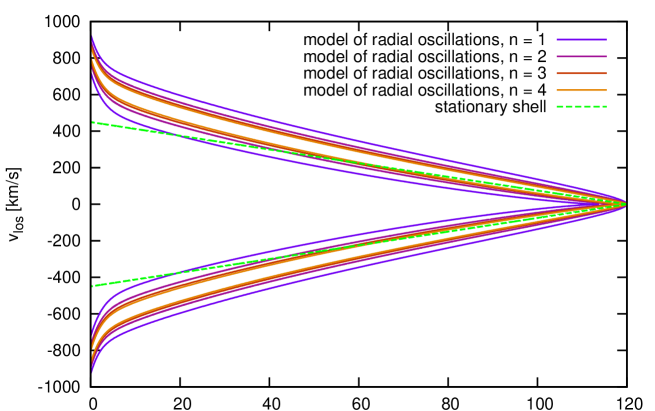
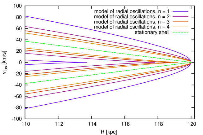
?figurename? 20: LOSVD peak locations for the stationary shell at the radius of 120 kpc according to Eq. (25) (green dashed lines); and for the first four shells at the radius of 120 kpc (parameters of the shells are listed in Table 2) according to the model of radial oscillations (Sect. 9.4). The upper panel shows the whole range of radii, the lower zooms in on the edge of the shell.

11 Constant acceleration and shell velocity

Now we will leave the stationary case and look at the kinematics of a moving shell. The nonzero velocity of the shell complicates the kinematics of shells in two aspects. Due to the energy difference between inward and outward stars at the same radius, the LOSVD peak is split into two, see Fig. 12, and the shell edge is not at the radius of the current turning point, but slightly further from the center of the host galaxy. In this section, we describe the LOSVD of such a shell using the assumption of a locally constant galactic acceleration together with the assumption of a locally constant shell phase velocity. We call it the approximation of constant acceleration and shell velocity. In addition, we assume that the velocity of stars at the edge of the shell is equal to the phase velocity of the shell.

This approximation is nothing but a modification of the model of radial oscillations for a constant acceleration and shell velocity and thus the concept that the stars behave as if they were released in the center of the host galaxy at the same time and their distribution of energies is continuous is still valid in this approximation.

11.1 Motion of a star in a shell system

The galactocentric radius of the shell edge is a function of time, $r_{\mathrm{s}}(t)$, where $t=0$ is the moment of measurement and $r_{\mathrm{s}}(0)=r_{\mathrm{s0}}$ is the position of the shell edge at this time. We assume following:

• stars are on strictly radial orbits

• locally constant value of the radial acceleration $a_{0}$ in the host galaxy potential

• a locally constant velocity of the shell edge $v_{\mathrm{s}}$¹³

• stars at the shell edge have the same velocity as the shell

The galactocentric radius of each star is at any time $r(t)$, while $t_{\mathrm{s}}$ is the time when the star could be found at the shell edge $r_{\mathrm{s}}(t_{\mathrm{s}})$. Then the equation of motion and the initial conditions for the star near a given shell radius are

$$\frac{\mathrm{d}^{2}r(t)}{\mathrm{d}t^{2}}=a_{0},$$ (36)

$$\left.\frac{\mathrm{d}r(t)}{\mathrm{d}t}\right|_{t=t_{\mathrm{s}}}=v_{\mathrm{s}},$$ (37)

$$r(t_{\mathrm{s}})=r_{\mathrm{s}}(t_{\mathrm{s}})=v_{\mathrm{s}}t_{\mathrm{s}}+r_{\mathrm{s0}}.$$ (38)

The solution of these equations is

$$r(t)=a_{0}(t-t_{\mathrm{s}})^{2}/2+v_{\mathrm{s}}(t-t_{\mathrm{s}})+r_{\mathrm{s}}(t_{\mathrm{s}}),$$ (39)

$$v_{r}(t)=v_{\mathrm{s}}+a_{0}(t-t_{\mathrm{s}}),$$ (40)

and the actual position of the star $r(0)$ and its radial velocity $v_{r}(0)$ at time of measurement ($t=0$) are

$$r(0)=t_{\mathrm{s}}^{2}a_{0}/2+r_{\mathrm{s0}},$$ (41)

$$v_{r}(0)=v_{\mathrm{s}}-a_{0}t_{\mathrm{s}}.$$ (42)

Eliminating $t_{\mathrm{s}}$ from the two previous equations, we get

$$v_{r}(0)_{\pm}=v_{\mathrm{s}}\pm v_{\mathrm{c}}\sqrt{2\left(1-r(0)/r_{\mathrm{s0}}\right)},$$ (43)

where $v_{\mathrm{c}}=\sqrt{-a_{0}r_{\mathrm{s0}}}$ is the circular velocity at the shell-edge radius.

11.2 Approximative LOSVD

The projection of the velocity given by Eq. (43) to the LOS at a projected radius $R$ will be

$$\begin{array}[]{rcl}v_{\mathrm{los}\pm}&=&\sqrt{1-R^{2}/\left(r\left(0\right)\right)^{2}}v_{r}(0)_{\pm}=\\ &=&\sqrt{1-R^{2}/\left(r\left(0\right)\right)^{2}}\left[v_{\mathrm{s}}\pm v_{\mathrm{c}}\sqrt{2\left(1-r(0)/r_{\mathrm{s0}}\right)}\right].\end{array}$$ (44)

Using this expression, we can model the LOSVD at a given projected radius for a given shell. For the proper choice of a pair of values $v_{\mathrm{c}}$ and $v_{\mathrm{s}}$, we can find a match with observed and modeled peaks of the LOSVD. When we use this approach, we call it the approximative LOSVD.

To model the approximative LOSVD by Eq. (44), we have to add an assumption about the radial dependence of the shell-edge density distribution, Eq. (13). We chose this function in the same manner as in the model of radial oscillations that is in a way that corresponds to constant number of stars at the edge of the shell. In Sect. 9.7 we have shown in the model of radial oscillations that a different choice of the radial dependence of the shell brightness changes neither the quadruple-peaked shape of the LOSVD of the shells, nor the positions of the maximal/minimal velocity which corresponds to the peaks of the LOSVD. This holds also for the approximative LOSVD, because the approximative LOSVD is very close to the LOSVD from the model of the radial oscillations, see Fig. 23. For the approximative LOSVD also holds that the inner peaks of the LOSVD disappear in the zone between the current turning points and the edge of the shell.

11.3 Radius of maximal LOS velocity

MK98 proved that near the edge of a stationary shell, $r_{s}$, the maximum intensity of the LOSVD is at the edge of the distribution. They also proved that the maximal absolute value of the LOS velocity $v_{\mathrm{los,max}}$ comes from stars at the galactocentric radius

$$r_{v\mathrm{max}}=\frac{1}{2}(R+r_{\mathrm{s0}}),$$ (45)

at each projected radius $R$.

For a moving shell, analogous equations are significantly more complex and a similar relation cannot be easily proven. Nevertheless, when we apply both results of MK98 we can show in examples (Figs. 22, 23, and others) that their use is valid, even for nonstationary shells. In the framework of the radial oscillations model (Sect. 9.4), we have shown that the peaks of the LOSVD occur at the edges of distributions of the near or the far half of the galaxy (Sect. 9.8). The inner peak corresponds to inward-moving stars and the outer one to outward-moving ones. This approach is used in the equations in Sect. 11.4. The maximal LOS velocity corresponds to the outer peak and the minimal to the inner one. Reasons and justification for use of Eq. (45) for $r_{v\mathrm{max}}$ are discussed in Sect. 11.6, point 2 (see also Fig. 21).

11.4 Approximative maximal LOS velocity

Using the results of MK98, we derive an expression for the maxima/minima of the LOS velocity corresponding to locations of the LOSVD peaks in observable quantities (i.e., the maxima/minima of the LOS velocity, the projected radius, and the shell radius) by substituting $r_{v\mathrm{max}}$ given by Eq. (45) for $r(0)$ in Eq. (44)

$$\begin{array}[]{rcl}v_{\mathrm{los,max}\pm}\!&=&\!\left(v_{\mathrm{s}}\pm v_{\mathrm{c}}\sqrt{1-R/r_{\mathrm{s0}}}\right)\,\times\\ &&\times\sqrt{1-4\left(R/r_{\mathrm{s0}}\right)^{2}\left(1+R/r_{\mathrm{s0}}\right)^{-2}}.\end{array}$$ (46)

For the measured locations of the LOSVD peaks $v_{\mathrm{los,max}+}$, $v_{\mathrm{los,max}-}$, projected radius $R$, and shell-edge radius $r_{\mathrm{s0}}$, we can express the circular velocity $v_{\mathrm{c}}$ at the shell-edge radius and the current shell velocity $v_{\mathrm{s}}$ by using inverse equations:

$$v_{\mathrm{c}}=\frac{\left|v_{\mathrm{los,max}+}-v_{\mathrm{los,max}-}\right|}{2\sqrt{\left(1-R/r_{\mathrm{s0}}\right)\left[1-4\left(R/r_{\mathrm{s0}}\right)^{2}\left(1+R/r_{\mathrm{s0}}\right)^{-2}\right]}},$$ (47)

$$v_{\mathrm{s}}=\frac{v_{\mathrm{los,max}+}+v_{\mathrm{los,max}-}}{2\sqrt{1-4\left(R/r_{\mathrm{s0}}\right)^{2}\left(1+R/r_{\mathrm{s0}}\right)^{-2}}}.$$ (48)

We call this approach the approximative maximal LOS velocity.

11.5 Slope of the LOSVD intensity maxima

Alternatively, the value of the circular velocity $v_{\mathrm{c}}$ at the shell-edge radius could be inferred from measurements of positions of peaks at two or more different projected radii for the same shell: let $\bigtriangleup v_{\mathrm{los}}=v_{\mathrm{los,max}+}-v_{\mathrm{los,max}-}$, where $v_{\mathrm{los,max}\pm}$ satisfy Eq. (46). Then, in the vicinity of the shell edge,

$$\begin{array}[]{rcl}\bigtriangleup v_{\mathrm{los}}&=&2v_{\mathrm{c}}\sqrt{\left(R/r_{\mathrm{s0}}-1\right)\left[1-4\left(R/r_{\mathrm{s0}}\right)^{2}\left(1+R/r_{\mathrm{s0}}\right)^{-2}\right]}\simeq\\ &\simeq&2(1-R/r_{\mathrm{s0}})v_{\mathrm{c}},\end{array}$$ (49)

and taking the derivative with respect to the projected radius

$$\frac{\mathrm{d}(\bigtriangleup v_{\mathrm{los}})}{\mathrm{d}R}=-2\frac{v_{\mathrm{c}}}{r_{\mathrm{s0}}},$$ (50)

which happens to be the same expression as Eq. 26 (equation (7) in MK98). Nevertheless, for a stationary shell, $\bigtriangleup v_{\mathrm{los}}$ is the distance between the two LOSVD intensity maxima of a stationary shell, whereas in this framework, it is the distance between the outer peak for positive velocities and the inner peak for negative velocities or vice versa. This equation allows us to measure the circular velocity in shell galaxies using the slope of the LOSVD intensity maxima in the $R\times v_{\mathrm{los}}$ diagram.

When we use this approach, we call it the use of the slope of the LOSVD intensity maxima. It requires us to measure the LOSVD for at least two different projected radii. In exchange, as we show in Sect. 13.3, that it promises a more accurate derivation of $v_{\mathrm{c}}$. However it does not allow the derivation of the shell velocity $v_{s}$. For this purpose, we can use Eq. (46) to derive a hybrid relation between the positions of the LOSVD peaks, the circular velocity at the shell-edge radius $v_{\mathrm{c}}$, and the shell velocity:

$$v_{\mathrm{s}}^{2}=v_{\mathrm{c}}^{2}(1-R/r_{\mathrm{s0}})+\frac{v_{\mathrm{los,max}+}v_{\mathrm{los,max}-}}{4\left(R/r_{\mathrm{s0}}\right)^{2}\left(1+R/r_{\mathrm{s0}}\right)^{-2}-1}.$$ (51)

If we insert the value of $v_{\mathrm{c}}$ derived from the measurement of the LOSVD intensity maxima into this equation, we can expect a better estimate of the phase velocity of the shell.

11.6 Comparison of approaches

The approximation of a constant radial acceleration in the host galaxy potential and shell phase velocity (Sect. 11) splits into three different analytical and semi-analytical approaches for obtaining values of the circular velocity $v_{\mathrm{c}}$ at the shell-edge radius and the shell phase velocity $v_{\mathrm{s}}$. Different approaches/models have a different color assigned. This color is used in Figs. 21–27 and 31–33 to represent the output of the corresponding approach. Here we summarize differences, advantages and disadvantages in these three approaches:

1. The approximative LOSVD (purple curves): For the given shell at the chosen projected radius, Eq. (44) is a function of only two parameters – $v_{\mathrm{c}}$ and $v_{\mathrm{s}}$. Assuming a radial dependence of the shell-edge density distribution, Eq. (44) allows us to plot the whole LOSVD (Sect. 11.2). However, computing the LOSVD and the positions of peaks requires a numerical approach in this framework. When deriving $v_{\mathrm{c}}$ and $v_{\mathrm{s}}$ from the observed LOSVD, we need to find a numerical solution to Eq. (44) and to search for a pair of $v_{\mathrm{c}}$ and $v_{\mathrm{s}}$, which matches the (simulated) data best.

2. The approximative maximal LOS velocities (orange curves): Eq. (46) supplies the positions of the peaks directly. It differs from the previous approximation in the assumption about the galactocentric radius $r_{v\mathrm{max}}$, from which comes the contribution to the LOSVD at the maximal speed. The assumption is that $r_{v\mathrm{max}}$ is given by Eq. (45), which was derived by MK98 for a stationary shell. This equation is actually only very approximate (see Fig. 21), but allows us to analytically invert Eq. (46) to obtain formulae for the direct calculation of $v_{\mathrm{c}}$ and $v_{\mathrm{s}}$ from the measured peak positions in the spectrum of the shell galaxy near the shell edge – Eqs. (47) and (48). Nevertheless, when measuring in the zone between the radius of the current turning points and the shell radius, we can expect very bad estimates of $v_{\mathrm{c}}$ and $v_{\mathrm{s}}$.

3. Using the slope of the LOSVD intensity maxima in the $R\times v_{\mathrm{los}}$ diagram: Eq. (50) cannot be used to draw theoretical LOSVD maxima for the given potential of the host galaxy, because it connects only the circular velocity in the host galaxy and the difference of the slopes of the LOSVD maxima. Moreover, the difference of the slopes alone does not allow us to determine the shell velocity, but we can use Eq. (51) as it is described in Sect. 11.5. Nevertheless it is this approach that gives the most accurate estimate of $v_{\mathrm{c}}$ when applied to simulated data, Sect. 13.3.

These methods can be compared with the model of radial oscillations described in Sect. 9.4 (plotted with light blue curves in the relevant figures). The model of radial oscillations uses thorough knowledge of the potential of the host galaxy. From it we extract the circular velocity at the shell-edge radius and the current shell velocity and we put them in the approximative relations derived in Sect. 11. We apply all the three approximations to the simulated data in Sect. 13.3.

?figurename? 21: Galactocentric radii $r_{v\mathrm{max}}$ that contribute to the LOSVD maxima according to Eq. (45), which was used in the derivation of the approximative maximal/minimal LOS velocities (Sect. 11.6, point 2) – orange curve, according to the approximative LOSVD (Sect. 11.6, point 1) – purple curves, and according to the model of radial oscillations (Sect. 9.4) – light blue curves for the second shell at 120 kpc (parameters of the shell are highlighted in bold in Table 2). For parameters of the host galaxy potential, see Sect. 8.1.

Fig. 21 shows a comparison of the radii that contribute to the LOSVD maxima according to the model of radial oscillations, the approximative LOSVD, and the approximative maximal LOS velocities. For the first two methods, the radius corresponding to the inner maxima of the LOSVD (which are the maxima created by the inward stars) is lower than that for the outer maxima, whereas Eq. (45) assumes the same $r_{v\mathrm{max}}$ for both inward and outward stars.

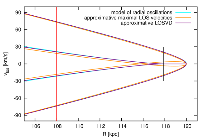
?figurename? 22: LOSVD peak locations for the second shell at the radius of 120 kpc (parameters of the shell are highlighted in bold in Table 2) according to the approximative maximal LOS velocities (Sect. 11.6, point 2) given by Eq. (46) (orange curves); the approximative LOSVD (Sect. 11.6, point 1) given by Eq. (44) (purple curves); and the model of radial oscillations (Sect. 9.4) (light blue curves which almost merged with the purple ones near the shell edge). The red line shows the position of the LOSVD from Fig. 23, the black one shows the position of the current turning points. The upper panel shows the whole range of radii, the lower zooms in on the edge of the shell. For parameters of the host galaxy potential, see Sect. 8.1.

Fig. 22 shows locations of the LOSVD peaks for the second shell at the radius of 120 kpc near the shell-edge radius. The purple curve is calculated using the approximative LOSVD (Sect. 11.6, point 1) given by Eq. (44), into which we inserted the velocity of the second shell according to the model of radial oscillations and the circular velocity in the potential of the host galaxy (see Sect. 8.1 for parameters of the potential). The purple curve does not differ significantly from the light blue curve calculated in the model of radial oscillations (Sect. 9.4). The more important deviations in the orange curve of the approximative maximal LOS velocities (Sect. 11.6, point 2) given by Eq. (46), are caused by Eq. (45) for $r_{v\mathrm{max}}$. With this assumption, approximative maximal LOS velocities (the orange curve) predict that around the zone between the current turning point and the shell edge, the inner peaks change signs. This means that for the part of the galaxy closer to the observer, both inner and outer peaks will fall into negative values of the LOS velocity and vice versa. However, from the model of the radial oscillations, we know that the signal from the inner peak in a given (near or far) part of the galaxy is always zero or has the opposite sign to that of the outer peak.

The model of the radial oscillations and the approximative LOSVD given by Eq. (44) were also used to construct the LOSVD for the second shell located at 120 kpc, at the projected radius of 108 kpc in Fig. 23. The graph also shows the locations of the peaks using the approximative maximal LOS velocities given by Eq. (46).

To wrap up, all three approaches give a good agreement with the model of radial oscillations. The first approach is practically identical to this model in the vicinity of the shell edge, but it requires numerical solution of equations. The second approach is more approximative and gives worse results particularly in the zone between the current turning point and the shell edge, but allows direct expression of $v_{\mathrm{c}}$ and $v_{\mathrm{s}}$. The third approach gives only the relation between the slopes of the LOSVD maxima and $v_{\mathrm{c}}$, but we have already announced that it gives the best results when calculating $v_{\mathrm{c}}$ from the simulated data.

?figurename? 23: LOSVD of the second shell at $r_{\mathrm{s}}=120$ kpc (parameters of the shell are highlighted in bold in Table 2) for the projected radius $R=0.9r_{\mathrm{s}}=108$ kpc according to the approximative LOSVD (Sect. 11.6, point 1) given by Eq. (44) (purple curve) and the model of radial oscillations (Sect. 9.4) (light blue curve almost merged with the purple one). Locations of peaks as given by the approximative maximal LOS velocities (Sect. 11.6, point 2) given by Eq. (46) are plotted with orange lines. Profiles do not include stars of the host galaxy that are not part of the shell system and are normalized, so that the total flux equals to one. For parameters of the host galaxy potential see Sect. 8.1.

11.7 Projection factor approximation

In Sect. 10.2 we have derived an approximative relation for the factor $z/r$ that projects the galactocentric velocity of the stars at radial trajectories to the line of sight, Eq. (29), which has been already used by Fardal et al. (2012) to derive the relation for $v_{\mathrm{los,max}\pm}$. Inserting this equation to the expression for the projected velocity of the stars of the shell, Eq. (44) in Sect. 11.2, we get

$$v_{\mathrm{los}\pm}(r)\simeq\sqrt{2(r/r_{\mathrm{s0}}-R/r_{\mathrm{s0}})}\left[v_{\mathrm{s}}\pm v_{\mathrm{c}}\sqrt{2\left(1-r/r_{\mathrm{s0}}\right)}\right].$$ (52)

?figurename? 24: Galactocentric radii $r_{v\mathrm{max\pm}}$ that contribute to the LOSVD maxima for the second shell at 120 kpc (parameters of the shell are highlighted in bold in Table 2) according to Eq. (53) – red curves. For comparison, we show the radii $r_{v\mathrm{max}}$ according to the model of radial oscillations (Sect. 9.4) – light blue curves – and according to the approximation of Sect. 11.6 (orange and purple curves). See also Fig. 21.

The derivative of this expression is zero for $r=r_{v\mathrm{max}\pm}$, where

$$r_{v\mathrm{max\pm}}=r_{\mathrm{s0}}\left(\frac{v_{\mathrm{s}}}{4v_{\mathrm{c}}}\right)^{2}\left[\frac{1}{2}\left(\frac{4v_{\mathrm{c}}}{v_{\mathrm{s}}}\right)^{2}\left(1+\frac{R}{r_{\mathrm{s0}}}\right)-1\pm\sqrt{\left(\frac{4v_{\mathrm{c}}}{v_{\mathrm{s}}}\right)^{2}\left(1-\frac{R}{r_{\mathrm{s0}}}\right)+1}\right].$$ (53)

Near the edge of the shell, the values $r_{v\mathrm{max\pm}}$ are in good coincidence with the galactocentric radii that contribute to the LOSVD maxima according to the model of radial oscillations (Sect. 9.4), whereas at lower radii they differ substantially, Fig. 24.

The position of the outer LOSVD peaks is expressed as the function $v_{\mathrm{los+}}(r_{v\mathrm{max+}})$, the position of the inner peaks as $v_{\mathrm{los-}}(r_{v\mathrm{max-}})$, Fig. 25. The equations have a solution only for $r_{v\mathrm{max}}<R$. The radius, where $r_{v\mathrm{max-}}=R$, is the radius of the current turning point $r_{\mathrm{TP}}$ in this approximation and for $R>r_{\mathrm{TP}}$ the inner peaks disappear. Eq. (53) implies

$$r_{\mathrm{TP}}=r_{\mathrm{s0}}\left[1-\frac{1}{2}\left(\frac{v_{\mathrm{s}}}{v_{\mathrm{c}}}\right)^{2}\right].$$ (54)

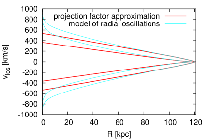
?figurename? 25: LOSVD peak locations for the second shell at the radius of 120 kpc (parameters of the shell are highlighted in bold in Table 2). The red curves show the values of the functions $v_{\mathrm{los+}}(r_{v\mathrm{max+}})$ and $v_{\mathrm{los-}}(r_{v\mathrm{max-}})$, where $v_{\mathrm{los\pm}}(r)$ is given by Eq. (52) and $r_{v\mathrm{max\pm}}$ follows Eq. (53). The light blue curves are LOSVD peak locations according to the model of radial oscillations (Sect. 9.4). The left panel shows the whole range of radii, the right zooms in on the edge of the shell. For parameters of the host galaxy potential, see Sect. 8.1.

The functions $v_{\mathrm{los+}}(r_{v\mathrm{max+}})$ and $v_{\mathrm{los-}}(r_{v\mathrm{max-}})$ are a good approximation to the LOSVD peak locations near the edge of the shell, as can be seen in Fig. 25. Using these functions are a better way to calculate these than the approximative LOSVD (Sect. 11.6, point 1), because their values are given analytically. Nevertheless they are such a complicated function of the circular velocity $v_{\mathrm{c}}$ at the shell-edge radius and the current shell velocity $v_{\mathrm{s}}$ that they do not allow the expression of these variables as a simple function of observable quantities, unlike the approximative maximal/minimal LOS velocities (Sect. 11.6, point 2). Thus we will not use these function in the following and show them only for the sake of completeness and comparison with Fardal et al. (2012).

12 Higher order approximation

The approximation of a locally constant galactic acceleration $a_{0}$ and shell phase velocity $v_{\mathrm{s}}$, Sect. 11, describes the positions of the LOSVD peaks fairly well and allows a good determination of the parameters of the potential of the host galaxy. Nevertheless we try to have a look outside the realm of constant $a_{0}$ and $v_{\mathrm{s}}$ using the same concept that stars behave as if they were released in the center of the host galaxy at the same time and their distribution of energies is continuous.

12.1 Motion of a star in a shell system

The galactocentric radius of the shell edge is a function of time, $r_{\mathrm{s}}(t)$, where $t=0$ is the moment of measurement and $r_{\mathrm{s}}(0)=r_{\mathrm{s0}}$ is the position of the shell edge at this time. Let us define a new coordinate system $s$, where the radial coordinate is the distance from the edge of the shell, in the same direction as the galactocentric radius

$$s(t)=r(t)-r_{\mathrm{s0}}.$$ (55)

The position of the stars of the given shell in this system is always negative.

We assume the following:

• stars are on strictly radial orbits

• radial acceleration in the potential of the host galaxy is given as $a(s)=a_{0}+a_{1}s$, where $a_{0}$ and $a_{1}$ are constant for a given shell

• position of the shell edge is (insofar) a general function of time $s_{\mathrm{s}}(t)$

• stars at the shell edge have the same velocity as the shell

The position of each star is at any time $s(t)$, while $t_{\mathrm{s}}$ is the time when the star could be found at the shell edge $s_{\mathrm{s}}(t_{\mathrm{s}})$. Then the equation of motion and the initial conditions for the star near a given shell radius are

$$\frac{\mathrm{d}^{2}s(t)}{\mathrm{d}t^{2}}=a_{0}+a_{1}s,$$ (56)

$$\left.\frac{\mathrm{d}s(t)}{\mathrm{d}t}\right|_{t=t_{\mathrm{s}}}=v_{\mathrm{s}},$$ (57)

$$s(t_{\mathrm{s}})=s_{\mathrm{s}}(t_{\mathrm{s}}).$$ (58)

The solution to these equation differs for negative and positive values of $a_{1}$. The position of a star in a general time $t$ is given by

$$s(t,a_{1}>0)=\frac{\left[a_{1}s_{\mathrm{s}}(t_{\mathrm{s}})+a_{0}\right]\cosh\left[\sqrt{a_{1}}\left(t-t_{\mathrm{s}}\right)\right]+\sqrt{a_{1}}v_{\mathrm{s}}\sinh\left[\sqrt{a_{1}}\left(t-t_{\mathrm{s}}\right)\right]-a_{0}}{a_{1}},$$ (59)

$$s(t,a_{1}<0)=\frac{\left[\left|a_{1}\right|s_{\mathrm{s}}(t_{\mathrm{s}})-a_{0}\right]\cos\left[\sqrt{\left|a_{1}\right|}\left(t-t_{\mathrm{s}}\right)\right]+\sqrt{\left|a_{1}\right|}v_{\mathrm{s}}\sin\left[\sqrt{\left|a_{1}\right|}\left(t-t_{\mathrm{s}}\right)\right]+a_{0}}{\left|a_{1}\right|},$$ (60)

where $\sinh(x)=1/2\left[\exp(x)-\exp(-x)\right]$ and $\cosh(x)=1/2\left[\exp(x)+\exp(-x)\right]$. For $a_{1}=0$, the solution of Sect. 11.1 holds. At the time of the measurement $t=0$ we obtain two pairs of equations for the position of the star $s(0)$ and its radial velocity $v_{r}(0)=\left.\mathrm{d}s(t)/\mathrm{d}t\right|_{t=0}$, depending on the sign of $a_{1}$

$$\begin{array}[]{rcl}s(0,a_{1}>0)&=&1/a_{1}\left\{\left[a_{1}s_{\mathrm{s}}(t_{\mathrm{s}})+a_{0}\right]\cosh\left(t_{\mathrm{s}}\sqrt{a_{1}}\right)-\sqrt{a_{1}}v_{\mathrm{s}}\sinh\left(t_{\mathrm{s}}\sqrt{a_{1}}\right)-a_{0}\right\},\\ v_{r}(0,a_{1}>0)&=&1/\sqrt{a_{1}}\left\{\sqrt{a_{1}}v_{\mathrm{s}}\cosh\left(t_{\mathrm{s}}\sqrt{a_{1}}\right)-\left[a_{1}s_{\mathrm{s}}(t_{\mathrm{s}})+a_{0}\right]\sinh\left(t_{\mathrm{s}}\sqrt{a_{1}}\right)\right\},\end{array}$$ (61)

$$\begin{array}[]{rcl}s(0,a_{1}<0)&=&1/\left|a_{1}\right|\left\{\left[\left|a_{1}\right|s_{\mathrm{s}}(t_{\mathrm{s}})-a_{0}\right]\cos\left(t_{\mathrm{s}}\sqrt{\left|a_{1}\right|}\right)-\sqrt{\left|a_{1}\right|}v_{\mathrm{s}}\sin\left(t_{\mathrm{s}}\sqrt{\left|a_{1}\right|}\right)+a_{0}\right\},\\ v_{r}(0,a_{1}<0)&=&1/\sqrt{\left|a_{1}\right|}\left\{\sqrt{a_{1}}v_{\mathrm{s}}\cos\left(t_{\mathrm{s}}\sqrt{\left|a_{1}\right|}\right)+\left[\left|a_{1}\right|s_{\mathrm{s}}(t_{\mathrm{s}})-a_{0}\right]\sin\left(t_{\mathrm{s}}\sqrt{\left|a_{1}\right|}\right)\right\}.\end{array}$$ (62)

For galactic potentials, one value of $s(0)$ will yield solutions for two different values of $t_{\mathrm{s}}$ and correspondingly two values of $v_{r}(0)$ and its projection to the line of sight. The minimal and maximal LOS velocities show the positions of LOSVD peaks.

12.2 Comparison of approximations

Now we compare this higher order approximation with the approximation of a constant acceleration (Sect. 11) and the model of radial oscillations (Sect. 9.4). For higher accuracy, we can obviously introduce the acceleration of the shell $a{}_{\mathrm{s}}$ and express the shell position as $s_{\mathrm{s}}(t_{\mathrm{s}})=v_{\mathrm{s}}t_{\mathrm{s}}+a{}_{\mathrm{s}}t_{\mathrm{s}}^{2}/2$. However, for observation data it would mean to fit 4 parameters ($a_{0}$, $a_{1}$, $v_{\mathrm{s}}$, and $a{}_{\mathrm{s}}$), what could prove difficult in practice. To compare the approximations, we thus restrict ourselves to a shell of constant velocity, that is $s_{\mathrm{s}}(t_{\mathrm{s}})=v_{\mathrm{s}}t_{\mathrm{s}}$, like in Sect. 11.

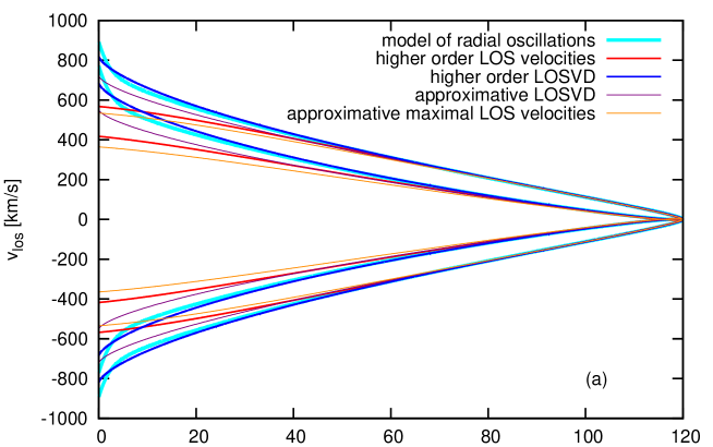
?figurename? 26: Comparison of LOSVD peak locations in different approximations for the second shell at the radius of 120 kpc, $a_{1}=1.2\times 10^{-5}$ Myr^-2. The upper panel shows the whole range of radii, the lower zooms in on the edge of the shell. For parameters of the host galaxy potential, see Sect. 8.1.

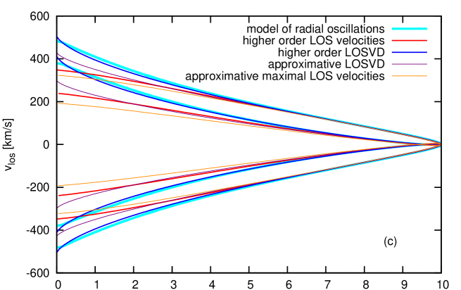
?figurename? 27: Comparison of LOSVD peak locations in different approximations for the first shell at the radius of 10 kpc, $a_{1}=8.5\times 10^{-4}$ Myr^-2. The upper panel shows the whole range of radii, the lower zooms in on the edge of the shell. For parameters of the host galaxy potential, see Sect. 8.1.

Besides the usual second shell at 120 kpc showed in Fig. 26, we show also the first shell at 10 kpc in Fig. 27. In our case, the value of $a_{1}$ at the galactocentric distance of 10 kpc is almost two orders of magnitude larger than the corresponding value at 120 kpc (see Fig. 28). For the approximations, we have used values of parameters calculated from the potential of the host galaxy (for parameters of the host galaxy potential, see Sect. 8.1). The model of radial oscillations (thick light-blue curves) requires the knowledge of the potential at all radii. The maxima/minima of the LOS velocities (that correspond to the locations of the peaks of the LOSVD) are shown in purple for the approximation of a constant acceleration (or, as we call it, using the "approximative LOSVD" by Eq. (44)), and in dark blue for a LOS projection of the solution of Eq. (61) with a nonzero $a_{1}$, which is positive for both shells. At the edge of the shell, both approximations are almost identical to the model of radial oscillations. On the other hand, at lower galactocentric radii, only the approximation with a nonzero $a_{1}$ follows the model of radial oscillations reasonably well. In general, the shell will be difficult to observe in real galaxies at lower projected radii, but for the case of observations of individual stars, star clusters and planetary nebulae, the kinematical imprint of the shell could be observed considerably far from its edge.

The purple and blue curves are calculated by finding maxima/minima of the LOS velocities at each projected radius. It is possible to obtain these in a much easier, but less accurate manner using the approximation for the radius of maximal LOS velocity $r_{v\mathrm{max}}=\frac{1}{2}(R+r_{\mathrm{s0}})$, as described in Sect. 11.3. The orange and red curves in Fig. 26 and Fig. 27 show the result of this procedure in the approximation of a constant acceleration (the "approximative maximal LOS velocity", Eq. (46)) and in the approximation with a nonzero value of $a_{1}$, respectively. Again, both approximations merge near the edge of the shell. For lower projected radii, the two curves separate again, but taking into account their overall difference from the model of radial oscillations, we cannot in this case consider the approximation of a nonzero $a_{1}$ to be a significant improvement. The approximative maximal LOS velocity with constant acceleration has the advantage that it allows a direct expression of basic variables (the circular velocity $v_{\mathrm{c}}$ at the shell-edge radius and shell phase velocity $v_{\mathrm{s}}$) in terms of observable quantities, facilitating and easy application to measured data. The same cannot be done in the approximation with a nonzero value of $a_{1}$.

12.3 $\boldsymbol{a{}_{1}}$

The assumption about the function $a(r)$ in the host galaxy is in fact an assumption on the radial dependence of the density of the host galaxy, by

$$a(r)=\frac{4\pi\mathrm{G}}{r^{2}}\int_{0}^{r}\rho(r^{\prime})r^{\prime 2}\mathrm{d}r^{\prime},$$ (63)

where $\rho(r)$ is the density in the host galaxy and G is the gravitational constant. For the case of constant acceleration $a=a_{0}$ the derivative of Eq. (63) with respect to $r$ shows that the density goes to zero for large $r$ as

$$\rho(r)=\frac{a_{0}}{2\pi\mathrm{G}}r^{-1},$$ (64)

whereas for $a=a_{0}+a_{1}(r-r_{\mathrm{s0}})$ the density goes to $\frac{3a_{1}}{4\pi\mathrm{G}}$ for large $r$ as

$$\rho(r)=\frac{3a_{1}}{4\pi\mathrm{G}}+\frac{a_{0}+a_{1}r_{\mathrm{s0}}}{2\pi\mathrm{G}}r^{-1}.$$ (65)

It is important to note that this approximation of the acceleration is applied only locally, although this word may sometimes mean a fairly large span of radii. The parameter $a_{1}$ may, in real galaxies, assume both positive and negative values. In Fig. 28 we show the radial dependence of $a_{1}$ in the host galaxy modeled as a double Plummer sphere (for parameters of the host galaxy potential, see Sect. 8.1).

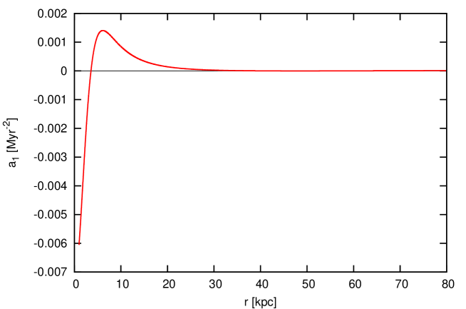
?figurename? 28: The radial dependence of $a_{1}$ in the host galaxy. For parameters of the host galaxy potential, see Sect. 8.1.

13 Test-particle simulation

We performed a simplified simulation of formation of shells in a radial minor merger of galaxies. Both merging galaxies are represented by smooth potential. Millions of test particles were generated so that they follow the distribution function of the cannibalized galaxy at the beginning of the simulation. The particles then move according to the sum of the gravitational potentials of both galaxies. When the centers of the galaxies pass through each other, the potential of the cannibalized galaxy is suddenly switched off and the particles continue to move only in the fixed potential of the host galaxy. We use the simulation to demonstrate the validity of our methods of recovering the parameters of the host galaxy potential by measuring the positions of the peaks in the LOSVD of simulated data.

?figurename? 29: Snapshots from our test-particle simulation of the radial minor merger, leading to the formation of shells. Each panel covers 300$\times$300 kpc and is centered on the host galaxy. Only the surface density of particles originally belonging to the satellite galaxy is displayed. The density scale varies between frames, so that the respective range of densities is optimally covered. Time-stamps mark the time since the release of the star in the center of the host galaxy.

In all cases, we look at the galaxy from the view perpendicular to the axis of collision, so that the cannibalized galaxy originally flew in from the right. Information on details of the simulation process can be found in Sect. 17.1.

13.1 Parameters of the simulation

The potential of the host galaxy is the same as the one described in Sect. 8.1. Let us only recall that it is a double Plummer sphere with respective masses $M_{*}=2\times 10^{11}$ M_⊙ and $M_{\mathrm{DM}}=1.2\times 10^{13}$ M_⊙ , and Plummer radii $\varepsilon_{*}=5$ kpc and $\varepsilon_{\mathrm{DM}}=100$ kpc for the luminous component and the dark halo, respectively. The potential of the cannibalized galaxy is chosen to be a single Plummer sphere with the total mass $M=2\times 10^{10}$ M_⊙ and Plummer radius $\varepsilon_{*}=2$ kpc.

The details of the simulations are described in Sect. 17.1. In the simulations that we present in this part, neither the gradual decay of the cannibalized galaxy nor the dynamical friction is included. The cannibalized galaxy is released from rest at a distance of 100 kpc from the center of the host galaxy. When it reaches the center of the host galaxy in 306.4 Myr, its potential is switched off and its particles begin to oscillate freely in the host galaxy. The shells start appearing visibly from about 50 kpc of galactocentric distance and disappear at around 200 kpc, as there are very few particles with apocenters outside these radii, Fig. 29. Video from the simulation is part of the electronic attachment. For the description of the video, see Appendix H point 2 and 3.

13.2 Comparison of the simulation with models

In the simulations, some of the assumptions that we used earlier (the model of radial oscillations, Sect. 9) are not fulfilled. First, the particles do not move radially, but on more general trajectories, which are, in the case of a radial merger, nevertheless very eccentric. Second, not all the particles are released from the cannibalized galaxy right in the center of the host galaxy; when the potential is switched off, the particles are located in the broad surroundings of the center and some are even released before the decay of the galaxy. These effects cause a smearing of the kinematical imprint of shells, as the turning points are not at a sharply defined radius, but rather in some interval of radii for a given time.

?figurename? 30: Simulated shell structure 2.2 Gyr after the decay of the cannibalized galaxy. Only the particles originally belonging to the cannibalized galaxy are taken into account. Top: surface density map; middle: the LOSVD density map of particles in the $\pm 1$ kpc band around the collision axis; bottom: histogram of galactocentric distances of particles. The angle between the radial position vector of the particle and the $x$-axis (the collision axis) is less than 90$\degr$ for the blue curve and less than 45$\degr$ for the red curve. The horizontal axis corresponds to the projected distance $X$ in the upper panel, to the projected radius $R$ in the middle panel, and to the galactocentric distance $r$ in the lower panel.

$r_{\mathrm{s}}$	$n$	$r_{\mathrm{TP,model}}$	$v_{\mathrm{s,sim}}$	$v_{\mathrm{s,model}}$	$v\mathrm{{}_{c,model}}$
kpc		kpc	km$/$s	km$/$s	km$/$s
48.8	5	48.5	38.7$\pm$2.1	38.7	326
$-$70.6	4	$-$69.9	59.8$\pm$1.6	54.3	390
105.0	3	103.9	68.1$\pm$1.9	63.5	441
$-$157.8	2	$-$155.7	74.3$\pm$1.2	72.4	450
257.4	1	251.0	97.5$\pm$1.4	95.7	406

?tablename? 3: Parameters of the shells in a simulation 2.2 Gyr after the decay of the cannibalized galaxy. The shell positions $r_{\mathrm{s}}$ are taken from the simulation. The values of $r_{\mathrm{TP,model}}$ and $v_{\mathrm{s,model}}$ are calculated for the shell position $r_{\mathrm{s}}$ and its corresponding serial number $n$ according to the model of radial oscillations (Sect. 9). The shell velocity $v_{\mathrm{s,sim}}$ is derived from 20 positions between the times 2.49–2.51 Gyr for each shell. The value $v\mathrm{{}_{c,model}}$ corresponds to the circular velocity at the shell-edge radius $r_{\mathrm{s}}$ for the chosen potential of the host galaxy (Sect. 8.1).

?figurename? 31: LOSVD map of the simulated shell structure 2.2 Gyr after the decay of the cannibalized galaxy (middle panel in Fig. 30). Light blue curves show locations of the maxima according to the model of radial oscillations (Sect. 9.4) for shell radius $r_{\mathrm{s}}$, corresponding serial number $n$, and the known potential of the host galaxy (Sect. 8.1). Orange curves are derived from the approximative maximal LOS velocities (Sect. 11.6, point 2) given by Eq. (46) for $r_{\mathrm{s}}$, $v_{\mathrm{s,model}}$, and $v\mathrm{{}_{c,model}}$. Parameters of the shells are shown in Table 3. Black lines mark the location at $0.9r_{\mathrm{s}}$ for each shell. The LOSVD for these locations are shown in Fig. 32. The map includes only stars originally belonging to the cannibalized galaxy.

The model of radial oscillations presented in Sect. 9 predicts that 2.2 Gyr after the decay of the cannibalized galaxy, five outermost shells should lie at the radii of 257.3, $-$157.8, 105.1, $-$70.5, and 48.8 kpc. The negative radii refer to the shell being on the opposite side of the host galaxy with respect to the direction from which the cannibalized galaxy flew in. These radii agree surprisingly well with the radii of the shells measured in the simulation 2.2 Gyr after the decay of the cannibalized galaxy, see Fig. 30 and Table 3. The position of the shell edge $r_{\mathrm{s}}$ in the simulation was determined as the position of a sudden decrease of the projected surface density (see Figs. 41 and  42). These values are shown in Table 3.

In the simulation, the first shell at 257.4 kpc is composed of only a few particles, and therefore we will not consider it (its parameters are listed in Table 3 for completeness). Thus, the outermost relevant shell in the system lies at $-$157.8 kpc and has a serial number $n=2$. Also, the shell at 48.8 kpc suffers from lack of particles, but we will include it nevertheless.

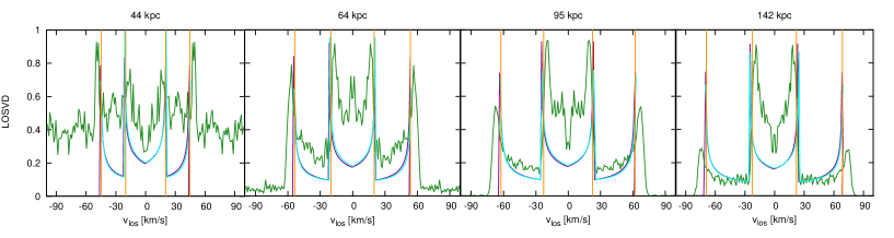
?figurename? 32: LOSVDs of four shells at projected radii $0.9r_{\mathrm{s}}$ (indicated as the title of each plot) 2.2 Gyr after the decay of the cannibalized galaxy (parameters of the shells are shown in Table 3). The simulated data are shown in green, the LOSVDs according to the approximative LOSVD (Sect. 11.6, point 1) given by Eq. (44) in purple, and LOSVDs according to the model of radial oscillations (Sect. 9.4) in light blue. The graph also shows the locations of the peaks using the approximative maximal LOS velocities (Sect. 11.6, point 2) given by Eq. (46) by orange lines. Profiles do not include stars of the host galaxy, which are not part of the shell system. The theoretical profiles are scaled so that the intensity of their highest peak approximately agrees with the highest peak of the simulated data. LOSVD is given in relative units, so maxima of the profiles have values of about 0.9.

Fig. 31 shows the comparison between the LOSVD in the simulation, the peaks of the LOSVD computed in the model of radial oscillations (light blue curves), and the approximative maximal LOS velocities – Eq. (46) (orange curves). To evaluate the approximative maximal LOS velocities, we obtained the shell velocity $v_{\mathrm{\mathrm{s,model}}}$ from the model of radial oscillations (Sect. 9) for the respective serial number $n$ of the shell and circular velocity $v\mathrm{{}_{c,model}}$ at the shell-edge radius, using our knowledge of the potential of the host galaxy. The values of all the respective shell quantities are listed in Table 3. Within the resolution of Fig. 31, the theoretical positions of the LOSVD maxima agree very well with the simulated data, even further from the shell edge than the usual limit of $0.9r_{\mathrm{s}}$.

Fig. 31 also shows the locations that correspond to the radii of $0.9r_{\mathrm{s}}$ for each individual shell (black lines). The LOSVD for these locations is shown in Fig. 32. The data are taken from an area spanning $0.5\times 2$ kpc centered at $(R,0)$ in the projected $X-Y$ plane, where $R$ is the number indicated above the corresponding panel in Fig. 32. The positions of simulated LOSVD peaks largely agree with the approaches of the approximation of constant acceleration and shell velocity described in Sect. 11.6 and with the model of radial oscillations (Sect. 9).

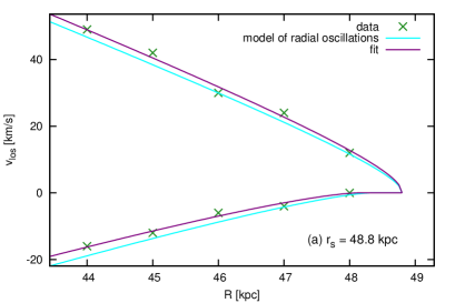
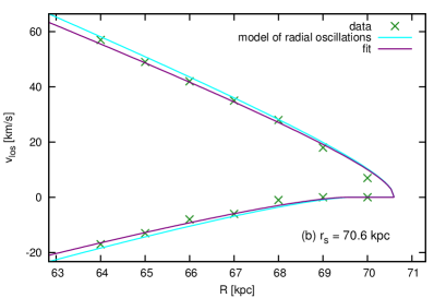
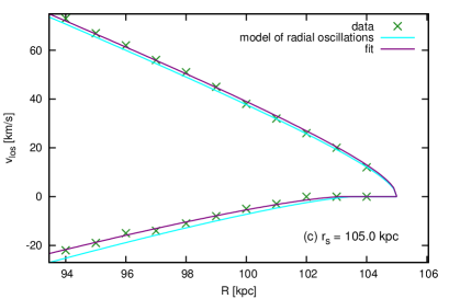
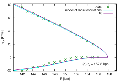
?figurename? 33: Fits for circular velocity $v_{\mathrm{c}}$ and shell velocity $v_{\mathrm{s}}$ using the approximative LOSVD (Sect. 11.6, point 1) given by Eq. (44) for four shells ($r_{\mathrm{s}}$ indicated in bottom right corner of each plot) in the simulation 2.2 Gyr after the decay of the cannibalized galaxy. The best fit is the purple curve, and its parameters are shown in Tables 4 and 5 in the columns labeled $v_{\mathrm{c,fit}}$ and $v_{\mathrm{s,fit}}$. The green crosses mark the measured maxima in the LOSVD, and the light blue curves show the locations of the theoretical maxima derived from the host galaxy potential according to the model of radial oscillations (Sect. 9.4). Note that the values of $v_{\mathrm{c}}$ and $v_{\mathrm{s}}$ used in the approximative LOSVD for the purple line were obtained by fitting the parameters to the simulated data, whereas in Figs. 22, 23, and 32, the values are known from the model of the host galaxy potential.

13.3 Recovering the potential from the simulated data

We used a snapshot from our simulation, which 2.2 Gyr after the decay of the cannibalized galaxy, as a source of the simulated data and tried to reconstruct the parameters of the potential of the host galaxy from the locations of the LOSVD peaks measured from the simulated data by using the the approximation of constant acceleration and shell velocity (Sect. 11).

For a given host galaxy, the signal-to-noise (S$/$N) ratio in the simulated data is a function of the number of simulated particles, the age of the shell system, the distribution function of the cannibalized galaxy, and the impact velocity. For a given radius in the simulated data, we can obtain arbitrarily good or bad S$/$N ratios by tuning these parameters. Thus, we adopted the universal criteria: 1) the LOSVD of each shell is observed down to 0.9 times its radius; 2) we measured the positions of the LOSVD peaks in different locations within the shell, sampled by 1 kpc steps. These criteria give us between 7 and 15 measurements for a shell. Each measurement contains two values: the positions of the outer and inner peaks, $v_{\mathrm{los,max}+}$ and $v_{\mathrm{los,max}-}$, respectively, for each projected radius $R$ (see green crosses in Fig. 33).

?figurename? 34: Comparison of velocity of the shell as a function of radius from the model and the simulated data. Velocity for the first shell ($n=1$) in the host galaxy model is shown by the black line. Red crosses show $v_{\mathrm{s,eq(\ref{eq:vs-vc})-slope}}$ (Table 5) as they result from the analysis of the simulated LOSVD. Values are corrected for shell number $n$ by the factor $3/(2n+1)$, so they correspond to velocity of the first shell, e.g., Eq. (5).

We do not estimate the errors, since the real data will be dominated by other sources, such as the contamination of the signal from the light of the host galaxy and the accuracy of the subtraction of this background light, night-sky background in the case of ground-based telescopes, detector noise, instrumental dispersion, accuracy in the determination of the systemic velocity and so forth. So we decided to quote only the mean square deviation and the standard error of the linear regression.

First we used the approximative maximal LOS velocities given by Eqs. (47) and (48) for a direct calculation of the circular velocity $v_{\mathrm{c,eq(\ref{eq:vc,obs})}}$ at the shell-edge radius $r_{\mathrm{s}}$ and the current shell velocity $v_{\mathrm{s,eq(\ref{eq:vs,obs})}}$. These equations are the inverse of Eq. (46), which corresponds to the model shown in orange lines in pictures throughout the text (Sect. 11.6, point 2). Mean values from all the measurements for each shell are shown in Tables 4 and 5 in the end of the section.

Compared with the approximative maximal LOS velocities, we obtain a better agreement with the circular velocity of our host galaxy potential when using the slope of the LOSVD intensity maxima (Sect. 11.6, point 3) given by Eq. (50), where we fit the linear function of the measured distance between the outer and the inner peak on the projected radius ($v_{\mathrm{c,slope}}$ in Table 4 and in Fig. 35). To estimate the shell velocity, we use a hybrid relation Eq. (51) between the positions of the LOSVD peaks, the circular velocity at the shell-edge radius $v_{\mathrm{c}}$, and the shell velocity. We substitute the values of $v_{\mathrm{c,slope}}$ derived from the measurements (that we know better describe the real circular velocity of the host galaxy) into this relation, thus obtaining the improved measured shell velocity $v_{\mathrm{s,eq(\ref{eq:vs-vc})-slope}}$ (Table 5 and Fig. 34).

In the zone between the current turning points and the shell edge, the inner peaks coalesce and gradually disappear (Fig. 15). The simulated data do not show a disappearance of the inner peaks as abrupt and clear as the theoretical LOSVD profiles predict, so that in this zone, we can usually measure one inner peak at 0 km$/$s. The information from these measurements is degenerate, and thus we defined a subsample of simulated measurements with all four clear peaks in the LOSVD (in the columns labeled SS in Tables 4 and 5). The spread of the values derived using the approximative maximal LOS velocities given by Eqs. (47) and (48) is significantly lower for the subsample ($v_{\mathrm{c,eq(\ref{eq:vs,obs})}}^{\mathrm{SS}}$ and $v_{\mathrm{s,eq(\ref{eq:vc,obs})}}^{\mathrm{SS}}$) due to the exclusion of areas where these equations do not hold well. On the contrary, the slope of the linear regression in Eq. (50) using the slope of the LOSVD intensity maxima gives a worse result (with a larger error) for the subsample $v_{\mathrm{c,slope}}^{\mathrm{SS}}$ than the approximative maximal LOS velocities.

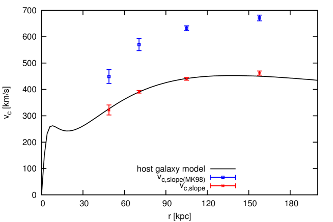
?figurename? 35: Circular velocity of the model and values derived from the simulated data: $v\mathrm{{}_{c,model}}$ of the host galaxy model is shown by the black line; blue and red points show values of circular velocity as they result from the analysis of the simulated LOSVD (see Sect. 13.2 and Table 4 for the numbers).

The third option to derive the circular velocity $v_{\mathrm{c}}$ at the shell-edge radius $r_{\mathrm{s}}$ and shell velocity $v_{\mathrm{s}}$ from the simulated data is to use the approximative LOSVD given by Eq. (44), which corresponds to the model shown in purple lines in pictures throughout the text (Sect. 11.6, point 1). However, this requires a numerical solution of the equation for a given pair of $v_{\mathrm{c}}$ and $v_{\mathrm{s}}$. We have calculated two sums of squared differences between $v_{\mathrm{los,max}}(v_{\mathrm{c}},v_{\mathrm{s}})$ as given by the approximative LOSVD and the simulated data. One for $v_{\mathrm{los,max-}}(v_{\mathrm{c}},v_{\mathrm{s}})$ and a second one for $v_{\mathrm{los,max+}}(v_{\mathrm{c}},v_{\mathrm{s}})$ . Then we have searched for the minimum of the sum of these two values to obtain best fitted values $v_{\mathrm{c,fit}}$ and $v_{\mathrm{s,fit}}$ (see Tables 4 and 5 for the results). Errors were estimated using the ordinary least squared minimization as if the functions $v_{\mathrm{los,max}+}(v_{\mathrm{c,fit}},v_{\mathrm{s,fit}})$ and $v_{\mathrm{los,max}-}(v_{\mathrm{c,fit}},v_{\mathrm{s,fit}})$ were fitted separately; quoted is the larger of the two errors.

$r_{\mathrm{s}}$	$v\mathrm{{}_{c,model}}$	$N$	$N^{\mathrm{SS}}$	$v_{\mathrm{c,eq(\ref{eq:vc,obs})}}$	$v_{\mathrm{c,eq(\ref{eq:vc,obs})}}^{\mathrm{SS}}$	$v_{\mathrm{c,slope}}$	$v_{\mathrm{c,slope}}^{\mathrm{SS}}$	$v_{\mathrm{c,fit}}$	$v_{\mathrm{c,slope(MK98)}}$
kpc	km$/$s			km$/$s	km$/$s	km$/$s	km$/$s	km$/$s	km$/$s
48.8	326	5	4	346$\pm$130	340$\pm$94	322$\pm$19	314$\pm$32	318$\pm$51	449$\pm$26
$-$70.6	390	7	5	394$\pm$85	390$\pm$53	391$\pm$5	392$\pm$11	368$\pm$60	570$\pm$23
105.0	441	11	8	478$\pm$144	452$\pm$64	440$\pm$5	447$\pm$7	427$\pm$28	632$\pm$9
$-$157.8	450	15	10	497$\pm$236	472$\pm$79	462$\pm$8	484$\pm$14	460$\pm$32	671$\pm$11

?tablename? 4: Circular velocity at the shell-edge radius $r_{\mathrm{s}}$ derived from the measurement of the simulated data 2.2 Gyr after the decay of the cannibalized galaxy. $r_{\mathrm{s}}$ and $v\mathrm{{}_{c,model}}$ have the same meaning as in Table 3. $N$: number of measurements for each shell; $v_{\mathrm{c,eq(\ref{eq:vc,obs})}}$: the mean of values derived from the approximative maximal LOS velocities given by Eq. (47) with its mean square deviation; $v_{\mathrm{c,slope}}$: a value derived from the linear regression using the slope of the LOSVD intensity maxima given by Eq. (50) and its standard error (see also Fig. 35); $v_{\mathrm{c,fit}}$: a value derived by fitting a pair of $v_{\mathrm{c}}$ and $v_{\mathrm{s}}$ in the approximative LOSVD given by Eq. (44) (Sect. 11.6, point 1 and Fig. 33); $v_{\mathrm{c,slope(MK98)}}$: the mean of values derived from the slope of the LOSVD intensity maxima given by Eq. (50) with its standard error (see also Fig. 35). In the equation, however, $\bigtriangleup v_{\mathrm{los}}$ is substituted with the distance between the two outer peaks of the LOSVD intensity maxima in order to mimic the measurement as originally proposed by MK98 for double-peaked profile. The quantities with the superscript SS correspond to the subsample, where only measurements with two discernible inner peaks in the LOSVD are used.

$r_{\mathrm{s}}$	$v_{\mathrm{s,model}}$	$v_{\mathrm{s,sim}}$	$v_{\mathrm{s,eq(\ref{eq:vs,obs})}}$	$v_{\mathrm{s,eq(\ref{eq:vs,obs})}}^{\mathrm{SS}}$	$v_{\mathrm{s,eq(\ref{eq:vs-vc})-slope}}$	$v_{\mathrm{s,eq(\ref{eq:vs-vc})-slope}}^{\mathrm{SS}}$	$v_{\mathrm{s,fit}}$
kpc	km$/$s	km$/$s	km$/$s	km$/$s	km$/$s	km$/$s	km$/$s
48.8	38.7	38.7$\pm$2.1	50.7$\pm$2.3	51.7$\pm$1.1	44.2$\pm$6.5	44.9$\pm$6.3	53$\pm$16
$-$70.6	54.3	59.8$\pm$1.6	60.8$\pm$9.8	65.6$\pm$2.0	60.7$\pm$10.8	66.0$\pm$2.9	66$\pm$19
105.0	63.5	68.1$\pm$1.9	74.8$\pm$4.6	76.5$\pm$1.4	68.0$\pm$8.9	71.3$\pm$2.5	79$\pm$9
$-$157.8	72.4	74.3$\pm$1.2	84.4$\pm$5.4	86.7$\pm$2.0	78.7$\pm$10.5	82.$\pm$3.5	85$\pm$14

?tablename? 5: Velocity of the shell at the radius $r_{\mathrm{s}}$ derived from the measurement of the simulated data 2.2 Gyr after the decay of the cannibalized galaxy. $r_{\mathrm{s}}$, $v_{\mathrm{s,model}}$, and $v_{\mathrm{s,sim}}$ have the same meaning as in Table 3. $v_{\mathrm{s,eq(\ref{eq:vs,obs})}}$: the mean of values derived from the approximative maximal LOS velocities given by Eq. (48) with its mean square deviation; $v_{\mathrm{s,eq(\ref{eq:vs-vc})-slope}}$: the mean of values derived from the hybrid relation given by Eq. (51) with its mean square deviation (see also Fig. 34); $v_{\mathrm{s,fit}}$: a value derived by fitting a pair of $v_{\mathrm{c}}$ and $v_{\mathrm{s}}$ in the approximative LOSVD given by Eq. (44) (Sect. 11.6, point 1 and Fig. 33). The quantities with the superscript SS correspond to the subsample, where only measurements with two discernible inner peaks in the LOSVD are used. Number of measurements is the same as in Table 4 for each shell.

The LOSVD intensity maxima resulting from this procedure are plotted in Fig. 33, together with the fitted data and the maxima given by the model of radial oscillations (Sect. 9.4). All three agree fairly well. The remaining two methods (the approximative maximal LOS velocities and using the slope of the LOSVD intensity maxima) use only equations to derive $v_{\mathrm{c}}$ and $v_{\mathrm{s}}$ and thus we do not show them in the plot. On the other hand, in Figs. 34 and 35, we show the comparison of values extracted from the simulated data with model values only for the most successful approach – using the slope of the LOSVD intensity maxima.

For the sake of comparison with the method of MK98, we calculated the circular velocity $v_{\mathrm{c,slope(MK98)}}$ at the shell-edge radius $r_{\mathrm{s}}$ using the slope of the LOSVD intensity maxima given by Eq. (50). To mimic the measurement of the circular velocity according to the Eq. (26), which was derived for the double-peaked profile, we assume $\bigtriangleup v_{\mathrm{los}}$ is the distance between the two outer peaks of the LOSVD intensity maxima. In Table 4 and Fig. 35, we can easily see that the values $v_{\mathrm{c,slope(MK98)}}$ differ from the actual circular velocity of the host galaxy $v\mathrm{{}_{c,model}}$ by a factor of 1.3–1.5.

The main message of this section is that in order to obtain the value of the circular velocity $v_{\mathrm{c}}$ at the shell-edge radius and shell phase velocity $v_{\mathrm{s}}$ from kinematical data near the shell edge, the best approach to use is the method based on the slope of the LOSVD intensity maxima given by Eq. (50) without limiting the data to a subsample.

13.4 Notes about observation

This work is a theoretical one, dealing with simulations and models. Obtaining and analyzing real data requires preparation, knowledge and experience that are beyond the goals we have set in this research. Nevertheless, we will make some remarks regarding potential observation of shell kinematics.

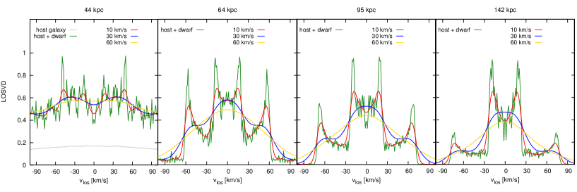
?figurename? 36: Line profiles of four shells at projected radii $0.9r_{\mathrm{s}}$ (indicated as the title of each plot, same as in Fig. 32) 2.2 Gyr after the decay of the cannibalized galaxy: gray lines show the LOSVDs for the host galaxy at a given radius (except for the radius of 44 kpc the signal of the host galaxy is negligible comparing to the signal from the cannibalized galaxy); green lines show the total LOSVDs from the host and the cannibalized galaxy together; red, blue, and yellow lines show convolutions of the total simulated data with different Gaussians representing the instrumental profiles having the FWHM 10, 30, and 60 km$/$s, respectively. Scaling is relative, similar as in Fig. 32.

When it comes to real observational data, there will be additional issues to deal with, night-sky background, detector noise, instrumental dispersion and so forth. MK98 estimated the data of the requisite quality could be obtained with a couple of nights integration using a 4-m telescope.

The situation gets more complex when the LOSVD assumes the quadruple-peaked profile instead of a double-peaked one. Not only becomes the intensity of a single peak smaller, but a higher spectral resolution is also needed to distinguish all four peaks. The instrumental dispersion naturally smooths features of the spectral profile. In Fig. 36, we show the LOSVDs from the simulated data smoothed with different Gaussians representing the instrumental profiles having the full width at half maximum (FWHM) of 10, 30, and 60 km$/$s. It is obvious that relatively high spectral resolution is necessary for observing an imprint of shell peaks in line profiles.

We have done our own simplified estimations of the observability of the LOSVD of shells. First, we used archival data of long-slit spectroscopy of the outermost shell in NGC 3923. The data were taken in July 2001 (about 10 hours of exposure time) and in March 2005 (about 20 hours) with FORS2 instrument at the Very Large Telescope (VLT, 8.2 meter diameter) of the European Southern Observatory. We processed a part of the data from 2005 using the FORS pipeline. The spectra are generally of a very low signal-to-noise ratio (S$/$N). We were particularly looking for the magnesium triplet around 5200 Å (taken into account the redshift of NGC 3923, about 30 Å) and we found no sign of it, so the analysis of kinematics was not possible. We conclude that the estimate of MK98 was probably a bit of an understatement.

Furthermore, we used exposure time calculators to determine expected S$/$N at available instruments (VLT/FORS2, VLT/FLAMES, Calar Alto/PPAK) assuming the exposure time 20 hours and the surface brightness of shells between 25 and 28 mag$/$arcsec² in V filter. The resulting S$/$N ranges from $\sim 0.3$ to $\sim 4.4$. This is not very satisfactory but using the integral field spectroscopy or the multi object spectroscopy, S$/$N could be increased by a factor of up to $\sim 10$ by summing the signal from all fibers. Moreover, one can use some kind of a cross-correlation technique (e.g., Simkin, 1974; Tonry and Davis, 1979) which allows to extract more accurate kinematic measurements than the actual resolution of the data is or extract more information from data with low S$/$N. Eventually, the situation should be much better with the next generation of telescopes, like the European Extremely Large Telescope or the James Webb Space Telescope.

Another important issue is the background light of the host galaxy. It is possible to model the LOSVD of the host galaxy, subtract it from the overall LOSVD and obtain the clear quadruple-peaked profile, but it may not be even necessary, because the velocity dispersion of the stars in the host galaxy would be likely significantly broader than the distance between the peaks and thus the peaks should be clearly visible already in the overall LOSVD.

Moreover, for shells at large radii, the contribution from the stars of the host galaxy becomes negligible – and it is exactly the shells at large radii that are the most interesting because our knowledge of the potential of the host galaxy is the worst in the outer parts of the galaxy, where the potential is expected to be dominated by the dark matter. In our simulated data, the host galaxy light is negligible already for the shell at 70 kpc, see Fig. 36. The surface brightness of observed shells goes from 24.5 mag$/$arcsec² (in V filter) up to the current detection limit of the deepest photometric observation $\sim 29$ mag$/$arcsec² (McGaugh and Bothun, 1990; Turnbull et al., 1999; Pierfederici and Rampazzo, 2004). The surface brightness of giant elliptical galaxies at $\sim 100$ kpc (the position of the outermost shell in NGC 3923) is 28–30 mag$/$arcsec² (in g and r filters; Tal and van Dokkum, 2011).

A category on its own is the measurement of LOS velocities of individual objects, such as globular clusters, planetary nebulae and individual giant stars (Fardal et al., 2012; Romanowsky et al., 2012), where the result is dependent only on the accuracy of the measurement and the number of measured objects.

The positions of LOSVD maxima should be symmetric around the systemic velocity which we can measure or assume to be in the middle between the peaks. We also need photometric data to find the center of the host galaxy and to measure the distance of the point of the spectroscopic observation and the shell edge from the center. As soon as we measure the locations of the LOSVD peaks $v_{\mathrm{los,max}+}$, $v_{\mathrm{los,max}-}$, the projected radius $R$ of the measurement, and the shell-edge radius $r_{\mathrm{s0}}$, we can calculate the value of the circular velocity $v_{\mathrm{c}}$ at the shell-edge radius and shell phase velocity $v_{\mathrm{s}}$ using one of the three approaches described in Sect. 11.6. Using the simulated data (Sect. 13.3), we found the derived $v_{\mathrm{c}}$ to be the most accurate when using the slope of the LOSVD intensity maxima given by Eq. (50), which requires the peak locations to be measured at several different radii. When a measurement from only one projected radius is available, Eqs. (47) and (48) can be used to derive $v_{\mathrm{c}}$ and $v_{\mathrm{s}}$ , respectively.

14 Shell density

In this section we take an apparent detour from the shell kinematics to explore the projected and volume densities of a shell. In Sect. 14.1 we express the projected surface density of the shell edge $\Sigma_{\mathrm{los}}(r_{\mathrm{s}})$ (that is, the projected surface density at the projected radius $R=r_{\mathrm{s}}$) as a function of $\Sigma_{\mathrm{sph}}$ (Sects. 9.6, 9.7, and 9.8) and the shell-edge radius $r_{\mathrm{s}}$. In Sect. 14.2 we investigate the evolution of $\Sigma_{\mathrm{los}}(r_{\mathrm{s}})$ as a function of time, as the position of the shell edge is a function of time. In Sect. 14.3 we show the volume density of a shell at a frozen moment and finally in Sect. 14.4, we explore the projected surface density of shells near the shell edge at a given time as a function of the projected radius $R$.

14.1 Projected surface density of the shell edge

Each time we needed to model an LOSVD, we have used the assumption that the shell-edge density distribution $\sigma_{\mathrm{sph}}\left(r_{\mathbf{s}}\right)$ or rather $\Sigma_{\mathrm{sph}}\left(r_{\mathbf{s}}\right)$ decreases as $1/r_{\mathrm{s}}^{2}\left(t\right)$, see Sects. 9.6, 9.7, and 9.8. Now we show how is this value related to an observable quantity, the projected surface density of the shell edge $\Sigma_{\mathrm{los}}(r_{\mathrm{s}})$. If we knew or assumed the mass-to-light ratio, $\Sigma_{\mathrm{los}}$ could be easily converted to the projected surface brightness.

?figurename? 37: Schema for the calculation of the projected surface density.

Consider a thin sphere of mass with a uniform spatial density $\rho$ and radius $r_{s}$, Fig. 37. When observed along the line of sight $z$, the amount of light registered from a point with a projected radius $R$ in the sphere’s image is proportional to the expression

$$\rho\Delta z=\rho\left(\sqrt{r_{\mathrm{s}}^{2}-R^{2}}-\sqrt{\left(r_{\mathrm{s}}-\Delta r\right)^{2}-R^{2}}\right),$$ (66)

which for an infinitesimally thin sphere ($\Delta r\rightarrow 0$) reduces to

$$\rho\Delta z\rightarrow\frac{r_{\mathrm{s}}\Sigma_{\mathrm{sph}}}{\sqrt{r_{\mathrm{s}}^{2}-R^{2}}}.$$ (67)

This expression diverges when the sphere is observed tangentially to its surface, that is on the shell edge – thus to talk about the projected surface density of the shell edge, we have to integrate the flux over a small observation area. As the shape of the area is irrelevant for infinitesimal sizes, we choose an area that is the easiest to integrate over in spherical coordinates that are convenient for a radially-symmetric density. Note that the angular size of the area is approximately $2\Delta R/r_{s}$ and thus the integrated flux is

$$\Sigma_{\mathrm{los}}=\frac{2}{S}\Sigma_{\mathrm{sph}}r_{\mathrm{s}}\intop_{0}^{\frac{\Delta R}{r_{\mathrm{s}}}}\intop_{r_{\mathrm{s}}-\Delta R}^{r_{\mathrm{s}}}\frac{R}{\sqrt{r_{\mathrm{s}}^{2}-R^{2}}}\mathrm{d}R\mathrm{d}\phi,$$ (68)

where $S=2\Delta R^{2}+o(\Delta R^{3})$ is the size of the integration area. Since $\intop_{a}^{b}\frac{x}{\sqrt{r^{2}-x^{2}}}\mathrm{d}x=\sqrt{r^{2}-b^{2}}-\sqrt{r^{2}-a^{2}}$, the integral reads

$$\Sigma_{\mathrm{los}}\simeq\Sigma_{\mathrm{sph}}\sqrt{\left(2r_{\mathrm{s}}-\Delta R\right)/\Delta R}\propto r_{\mathrm{s}}^{1/2}\Sigma_{\mathrm{sph}}.$$ (69)

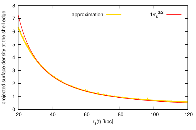
?figurename? 38: Time evolution of the projected surface density of the shell edge (0.01 kpc) in the approximation of a constant radial acceleration in the host galaxy potential and shell phase velocity (Sect. 11) – yellow curve, in arbitrary units. The red curve represents a function $r^{-3/2}$ normalized so that it has the same value at $R=60$ kpc as the yellow curve. For the parameters of the host galaxy potential, see Sect. 8.1.

?figurename? 39: Histogram of apocenters of particles in the simulation used in Sect. 13.

14.2 Time evolution

The radial dependence of $\Sigma_{\mathrm{sph}}$ is chosen, as usual, as $\Sigma_{\mathrm{sph}}(r_{\mathrm{s}}(t))\propto 1/r_{\mathrm{s}}^{2}(t)$. Then from Eq. (69) it follows that

$$\Sigma_{\mathrm{los}}(r_{\mathrm{s}}(t))\propto r_{\mathrm{s}}^{-3/2}(t).$$ (70)

However, the calculation leading to Eq. (69) assumes that all the stars are located at the sphere with the radius of the shell. We have thus examined the time evolution of the projected surface density of the shell edge in the framework of the approximation of a constant radial acceleration in the host galaxy potential and shell phase velocity (Sect. 11, in this section, Sect. 14, hereafter the approximation) – Fig. 38. For each shell radius we calculate the motion of stars under a constant acceleration, but we update this acceleration for different shell radii according to the chosen potential of the host galaxy (for the parameters of the potential, see Sect. 8.1). The time evolution of the projected surface density of the shell edge in this approximation does not depend on its velocity and thus on its serial number, see Sect. 14.4. In this approximation, stars are present at all radii, 0–$r_{\mathrm{s}}$, in contrast to the calculation that lead us to Eq. (70), where we assumed the stars to be located only at the shell radius (in a given time). Nevertheless, the time evolution of $\Sigma_{\mathrm{sph}}(r_{\mathrm{s}}(t))$, Fig. 38, turns out to be essentially identical when calculated by either of these approaches.

Both the calculation of Eq. (70), and the approximation assume $\Sigma_{\mathrm{sph}}$ to decrease as $1/r_{\mathrm{s}}^{2}\left(t\right)$, corresponding to constant number of stars at the edge of the shell, $N\left(r_{\mathbf{s}}\right)$. Fig. 39 shows the distribution of apocenters of particles in the simulation from Sect. 13, which is a good approximation to real $N\left(r_{\mathbf{s}}\right)$. We have to honestly admit that this function is anything but constant, but it is difficult to devise any approximation as the shape of the distribution significantly varies with parameters of the collision. Moreover, we do apply this function usually only in a small range of radii and as we have already shown, the character of the LOSVD does not depend much on its choice (Sects. 9.7 and 9.8). Converting the histogram of apocenters of the particles to the shell brightness is not straightforward as, both in the simulation and real shell galaxies, the distribution of particles is not uniform in azimuth, contrary to what he assumed in modeling the LOSVD both in the approximation and in the model of radial oscillations (Sect. 9.4).

14.3 Volume density

The calculation in Sect. 14.1 assumes that stars are at each moment located only on a sphere with the radius of the shell. Nevertheless it gives good results when compared to the approximation (Fig. 38), where this assumption does not hold. The reason is that the volume density decreases quickly inward from the shell edge (it obviously decreases outward in a jump, but that is not of concern at the moment). In their work, Hernquist and Quinn (1988) recall that Arnold (1984) states that for phase wrapped shells, that are just caustics in the mapping of the particle density from phase space into three-dimensional space, it holds that the density behind a caustic should scale as $(r_{\mathrm{s}}-r)^{-1/2}$. This behavior should be independent of the used potential of the host galaxy. In Fig. 40 we have compared the volume density near the shell edge in the approximation with this function and they indeed show a pretty good agreement.

?figurename? 40: Volume density for the third shell at $105$ kpc in the approximation of a constant radial acceleration in the host galaxy potential and shell phase velocity (Sect. 11) – yellow curve, in arbitrary units. The red curve represents a function $(r_{\mathrm{s}}-r)^{-1/2}$ normalized so that at $r_{\mathrm{s}}-r=1.1$ kpc it has the same value as the yellow curve. For the parameters of the host galaxy potential, see Sect. 8.1.

For a stationary shell, the volume density near the shell edge holds

$$\rho(r)=\frac{k}{v_{r}r^{2}},$$ (71)

where $k$ is a constant for the given shell and $v_{r}$ is the radial velocity of the shell. In a field of constant acceleration $a_{0}$ Eq. (27) holds – $v_{r}=\sqrt{2a_{0}(r-r_{\mathrm{s}})},$ thus the volume density is

$$\rho(r)\propto\frac{1}{r^{2}\sqrt{r-r_{\mathrm{s}}}}.$$ (72)

In the vicinity of the shell, the term $(r_{\mathrm{s}}-r)^{-1/2}$ dominates. For a moving shell it is difficult to make such analysis, but we have seen on an example, in Fig. 40, that this holds even in such case.

14.4 Projected surface density

Finally we reach a really observable quantity that is the projected surface density on the sky for a shell in a given time. For volume density following Eq. (72) the projected surface density turns out to be constant after integration. Thus we can assume constant projected surface density/brightness immediately behind the shell. The sharp-edged appearance of shells is caused by the abrupt decrease of their brightness outside the shell radius, as we already demonstrated in Sect. 9.3.

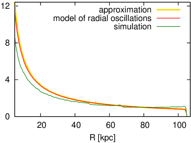
?figurename? 41: Surface brightness profile for two shells from simulation used in Sect. 13 – green curve; for equivalent shells using the approximation (Sect. 11) – yellow curve, and the model of radial oscillations (Sect. 9) – red curve. The curves are normalized so that they coincide and assume unit value at 50 and 80 kpc for shells with radii 70 and 105 kpc, respectively.

Fig. 41 shows the projected surface density profile for two shells from the simulation (Sect. 13) and for shells on same radii (70 and 105 kpc) using the approximation and the model of radial oscillations (Sect. 9). The approximation departs from the model of radial oscillations slightly only in the vicinity of the center of the host galaxy. In the approximation, the current location of a star for different $t_{\mathrm{s}}$ does not depend on the shell velocity, see Eq. (41), where $t_{\mathrm{s}}$ is the time where the star was or will be at the shell edge. Thus even the projected surface density calculated in the approximation does not depend on the serial number of the shell. The character of the profile immediate behind the shell is however slowly rising toward the center of the host galaxy, rather than constant. The shapes of the profile from the simulation and the approximation or the model of the radial oscillations coincide fairly well, even though the approximation and the model of radial oscillations assume uniform azimuthal distribution of particles which is obviously not valid in the simulation (see e.g. Figs. 30 or 29).

?figurename? 42: Surface brightness profile near the shell edge for the outer shell from simulation used in Sect. 13 – green curve; and for equivalent shells using the approximation – yellow curve, and the model of radial oscillations – red curve. The curves are normalized so that they coincide and assume unit value at 100 kpc.

On the other hand, no agreement at all is found for the outermost shell from the simulation at 158 kpc near its edge with the approximation or the model of radial oscillations, Fig. 42. The simulated shell even significantly decreases in brightness just at its edge. The reason for this is that the shell is nearing its demise and stars to arrive at higher radii are missing (see Figs. 30). Another factor is the azimuthal development of brightness, as the shell is the brightest near the axis of the merger and at higher angles (measured from the axis of the merger) the number of stars decreases. That, together with a large shell radius causes a decrease in the projected surface density at radii lower than the shell radius. A universal profile of the projected surface density/brightness for phase wrapped shells thus does not exist, but in general a rather constant or rising behavior can be expected for the inner shells, whereas the outer shell can show decrease toward the center of the host galaxy.

All the profiles of the projected surface density have been drawn for a band $\pm 1$ kpc around the merger axis in the projected plane perpendicular to the merger axis.

15 Discussion

In this part of the thesis, we developed a method to measure the potential of shell galaxies from kinematical data, extending the work of MK98, assuming a constant shell phase velocity and a constant radial acceleration in the host galaxy potential for each shell. The method splits into three different analytical and semi-analytical approaches (Sect. 11.6) for obtaining the circular velocity in the host galaxy, $v_{\mathrm{c}}$, and the current shell phase velocity, $v_{\mathrm{s}}$ – the approximative LOSVD, the approximative maximal LOS velocities, and the slope of the LOSVD intensity maxima. In Sect. 11.6, the first two approaches are compared to the model of radial oscillations (numerical integration of radial trajectories of stars in the host galaxy potential, Sect. 9). All three approaches are then applied to data for the four shells obtained from a test-particle simulation and compared to the theoretical values (Sect. 13.2).

The approximative LOSVD requires a numerical solution to Eq. (44) and the search for a pair of $v_{\mathrm{c}}$ and $v_{\mathrm{s}}$, which matches the (simulated) data best. Although this approach is not limited by any assumptions about the radius of the maximal LOS velocity (Sect. 11.3), it does not give a better estimate of $v_{\mathrm{c}}$ and $v_{\mathrm{s}}$ for our simulated shell galaxy than the other two methods. The deviation from the real value of $v_{\mathrm{c}}$ is between 2 % and 6 %.

Using the approximative maximal LOS velocities results in simple analytical relations and is the only one that can in principle be used for a LOSVD measured at only one projected radius. Nevertheless, when measuring in the zone between the radius of the current turning points and the shell radius, we can expect very bad estimates of $v_{\mathrm{c}}$ and $v_{\mathrm{s}}$. The mean value from more measurements of the LOSVD peaks for each shell of our simulated shell galaxy has similar accuracy to those of the approximative LOSVD, provided that we include only the measurements outside the zone between the radius of the current turning points and the shell radius.

The best method for deriving the circular velocity in the potential of the host galaxy seems to be to use the slope of the LOSVD intensity maxima, with a typical deviation in the order of units of km$/$s when fitting a linear function over all the measured positions of the LOSVD peaks for each shell. This circular velocity is then used in the hybrid relation, Eq. (51), to obtain the best estimate of the shell phase velocity.

All the approaches, however, derive the shell phase velocity systematically larger than the prediction of the model of radial oscillations $v_{\mathrm{s,model}}$ and the value derived from positions between the times 2.49–2.51 Gyr in the simulation $v_{\mathrm{s,sim}}$ (Table 5). This is because the simulated LOSVD peaks lie too far out (for the outer peaks) or too far in (for the inner peaks) when compared to the model of radial oscillations. That can be caused by nonradial trajectories of the stars of the cannibalized galaxy or by poor definition of the shell radius in the simulation.

Nevertheless, the shell phase velocity depends, even in the simplified model of an instant decay of the cannibalized galaxy in a spherically symmetric host galaxy (Sec. 9), on the serial number of the shell $n$ and on the whole potential from the center of the galaxy up to the shell radius, Eq. (5). A comparison of its measured velocity to theoretical predictions is possible only for a given model of the potential of the host galaxy and the presumed serial number of the observed shells. In such a case, however, it can be used to exclude some parameters or models of the potential that would otherwise fit the observed circular velocity.

The first shell has a serial number equal to one. A higher serial number means a younger shell. On the same radius, the velocity of each shell is always smaller than that of the previous one. In practice, it is difficult to establish whether the outermost observed shell is the first one created, or whether the first shell (or even the first couple of shells) is already unobservable. Here, we can use the potential derived from our method or a completely different one in a reverse way: to determine the velocity of the first shell on the given radius and to compare it to the velocity derived from the positions of the LOSVD peaks. Knowing the serial number of the outermost shell and its position allows us then to determine the time from the merger and the impact direction of the cannibalized galaxy. Moreover, the measurement of shell velocities can theoretically distinguish the shells from different generations, which can be present in a shell galaxy (Bartošková et al., 2011).

Our method for measuring the potential of shell galaxies has several limitations. Theoretical analyses were conducted over spherically symmetric shells, while the test-particle simulation was run for a strictly radial merger and analyzed in a projection plane parallel to the axis of the merger. In addition, both analytical analyses and simulations assume spherical symmetry of the potential of the host galaxy. In reality, the regular shell systems with higher number of shells in a single host galaxy are more often connected to galaxies with significant ellipticity (Dupraz and Combes, 1986). Moreover, in cosmological simulations with cold dark matter, halos of galaxies are described as triaxial ellipsoids (e.g., Jing and Suto, 2002; Bailin and Steinmetz, 2005; Allgood et al., 2006). However, the effect of the ellipticity of the isophotes of the host galaxy on the shell kinematics need not be dramatic, as the shells have the tendency to follow equipotentials that are in general less elliptical than the isophotes. Dupraz and Combes (1986) concluded that while the ellipticity of observed shells is generally low, it is neatly correlated to the eccentricity of the host galaxy. Prieur (1988) pointed out that the shells in NGC 3923 are much rounder than the underlying galaxy and have an ellipticity that is similar to the inferred equipotential surfaces. This idea was originally put forward by Dupraz and Combes (1986), who found such a relationship for their merger simulations. Our method is in principle applicable even to shells spread around the galactic center, which are usually connected to rounder elliptical galaxies if they were created in a close-to-radial merger. Nevertheless, the combination of the effects of the projection plane, merger axis, and ellipticity of the host galaxy can modify our results and require further analyses.

Because the kinematics of the stars that left the cannibalized galaxy is in the first approximation a test-particle problem, they should not be much affected by self-gravity of the cannibalized galaxy and the dynamical friction that this galaxy undergoes during the merger, both of which have been neglected in Part II.

Another complication is that the spectral resolution required to distinguish all four peaks is probably quite high (Sect. 13.4 and Fig. 36) and the shell contrast is usually small. The higher order approximation, Sect. 12, is sensible only when kinematical data are available to larger distances from the shell edge. In the application to simulated data, we considered a shell that is observable down to 0.9 shell radii. Nevertheless, there is the possibility to measure shell kinematics using the LOS velocities of individual globular clusters, planetary nebulae, and, in the Local group of galaxies, even of individual stars. It is even possible that the shell kinematics will be detectable in H I and CO emission, see Sects. 3.5 and 6.7.

We have also explored the projected surface density of shells, Sect. 14.4. In the model of radial oscillations, the shells show constant projected surface density near the shell edge, whereas outside the shell radius, there is a step-like decrease of the density, creating the sharp-edged feature of the shells. This behavior can be expected from shells with a large development in azimuth and a sufficient supply of stars at different energies. Already in our simple simulation of a radial minor merger with test particles and instantaneous decay of the cannibalized galaxy, we can observe a shell with a projected surface density that defies this description. We can assume that the self-gravity and gradual decay of the cannibalized galaxy can disrupt the observed profile even further. Moreover, we worked only in strictly spherical potentials and any non-zero ellipticity of the host galaxy can play a significant role. For the moment, all we can say is how the projected surface density of shells looks within the model of radial oscillations – any stronger statement would require more detailed simulations.

?partname? III Dynamical friction and gradual disruption

In the same spirit as in Part II, we will consider the formation of the shell structure during a radial minor merger. This time, we will try to get closer to real shell galaxies by introducing into the test-particle simulations the gradual decay of the secondary galaxy as well as its braking by dynamical friction against the primary.

16 Motivation

In Sect. 9.1 we have shown how are the positions of the shells related to the potential of the host galaxy at different times from the merger that created the shells. In practice, nevertheless, it has proven difficult to reproduce the space distribution of the shells in the observed shell galaxies using sensible potentials (Sect. 6). The main suspects of making the relation more complex are the dynamical friction and the possibility to have shells from multiple generations. In the case when the measurement of shell kinematics is not available, we can pose a goal less ambitions than the derivation of the potential of the host galaxy, that is to determine the age of the shell system (the time of the merger). To this end, the measurement of the position of the outermost shell could be sufficient, as this shell is the one which is the least effected by those additional effects.

As we have mentioned in Sect. 1, this is the approach chosen by Canalizo et al. (2007). They presented observations of shells in a quasar host galaxy and, by simulating the position of the outermost shell by means of restricted $N$-body simulations, attempted to put constraints on the age of the merger. They concluded that it occurred a few hundred Myr to $\sim 2$ Gyr ago, supporting a potential causal connection between the merger, the post-starburst ages in nuclear stellar populations, and the quasar. A typical delay of 1–2.5 Gyr between a merger and the onset of quasar activity is suggested by both $N$-body simulations by Springel et al. (2005) and observations by Ryan et al. (2008). It might therefore appear reassuring to find a similar time lag between the merger event and the quasar ignition in a study of an individual spectacular object.

The issue here is that noone has studied in detail the effects assumed to complicate the shell distribution (the dynamical friction and the gradual decay of the secondary galaxy) and thus it is not clear how exactly they change the shell structure and how they influence the position of the outermost shell. We try to include the dynamical friction and the gradual decay of the cannibalized galaxy in test-particle simulations. The manifestation of these processes in self-consistent simulations is difficult to separate and sometimes they may even be confused with non-physical outcomes of used methods. Test-particle simulations helped us to separate and better understand the roles of the dynamical friction and gradual tidal decay in the shell formation. Moreover, self-consistent simulations become demanding on computation time when we want to explore a significant part of the parameter space.

We look at what these enhanced test-particle simulations tell us about the potential and merger history of shell galaxies with the focus on the plausibility of the use of the outermost shell for dating the merger.

17 Description of simulation

In this and the previous part we show results of test-particle simulations and in this section we describe the procedure of their calculation in detail.

17.1 Configuration

The test (i.e. mass-less) particles of the secondary galaxy are generated (usually in counts from $10^{4}$ to $10^{7}$) so that they follow the density profile of the secondary galaxy. The particles then move according to a smooth gravitational potential of both galaxies, which move with respect to each other based on their masses, shape of potentials, positions and velocities; Eq. (77). Figures and videos are generally oriented so that the secondary galaxy approaches originally from the right hand side.

In the simplest case, when the centers of the galaxies pass through each other, the potential of the secondary galaxy is suddenly switched off and the particles continue to move only in the fixed potential of the primary galaxy. This approach is applied in simulation in Part II and in some simulations in Part III. In the simulations with dynamical friction and gradual disruption, the smooth potential of the secondary galaxy is kept for whole time and its mass is progressively lowered during each successive passage. The dynamical friction is added in the form of an (semi-)analytical prescription into the equations of motion of galaxies.

All the simulations in the thesis are, for the sake of simplicity, carried out for spherical galaxies, i.e. elliptical galaxies with zero ellipticity. The secondary (cannibalized) galaxy is always modeled as a single Plummer sphere. The primary (host) galaxy is modeled as a single or double Plummer sphere in Part III, while in Part II its potential has always two components, both Plummer spheres.

For the numerical integration of the motion of the test particles and the galaxies, the Leapfrog method was chosen. In this method, velocities derived for a time half step earlier (or later) than the current position are used to update the position. Conversely, to update the half-step velocity one step forward, the positions for the round position in between are used. In so doing the velocities can be seen to “leapfrog” over the current time step. This simple enterprise improves the accuracy of the numerical computation by an order compared to when the position $x$ and velocities $v$ are taken simultaneously. The error is of the order of $(\bigtriangleup t)^{3}$, where $\Delta t$ is the time step. For the longest time step used in our simulations (1 Myr), the error for the trial circular motion was only 11 revolutions after 10,000 (compared to the simple analytical solution that is available in this case), what is only 1 per mille.

17.2 Plummer sphere

The gravitational potential of each of the galaxies in this part, Part III, is modeled with the Plummer profile with varying parameters in different simulations:

$$\phi(r)=-\frac{\mathrm{G}\,M}{\sqrt{r^{2}+\varepsilon^{2}}},$$ (73)

where G is the gravitational constant, $M$ is the total mass of the galaxy, $r$ is the distance from the center of the galaxy and $\varepsilon$ is the Plummer radius – a scale parameter that determines the compactness of the galaxy. For $\varepsilon$ = 0 the Eq. (73) represents a simple potential of a point mass. The Plummer radius corresponds to the effective radius of the galaxy.

While the Plummer model follows the profile of the real spherical galaxies only approximately, we use it here – as was the case of numerous other studies of galaxies – because of its simple expressions of dynamical quantities. It was first used by Plummer (1911) to fit the observations of globular clusters and now is often used as a stellar distribution model in simulations.

From the Poisson equation $\bigtriangleup\phi=4\pi\mathrm{G}\rho$, we can easily infer the radial density distribution $\rho$ that acts as the source for the Plummer potential:

$$\rho(r)=\rho_{0}\frac{1}{(1+r^{2}/\varepsilon^{2})^{5/2}},$$ (74)

where $\rho_{0}=3M/(4\pi\varepsilon^{3})$ is the central density. About $\sqrt{2}/4$ (approx. 35%) of the total mass of the galaxy is enclosed inside the $r=\varepsilon$ radius.

The force $F(r)$ acting on a test particle (of a mass m) is calculated from the potential by the equation $F(r)=-\bigtriangledown\phi(r)$, what reads in Plummer potential as:

$$F(r)=-\mathrm{G}\,M\,m\frac{r}{(r^{2}+\varepsilon^{2})^{3/2}}.$$ (75)

The particles in our model then move according to an acceleration $\mathbf{a}(\mathbf{r})$ given by the potentials of both galaxies

$$\mathbf{a}(\mathbf{r})=-\mathrm{G}\sum_{i}\frac{M_{i}\mathbf{r}_{i}}{(r_{i}^{2}+\varepsilon_{i}^{2})^{3/2}},$$ (76)

where the summation goes over pres quantities corresponding to the secondary galaxy, and one or two components of the primary galaxy. In simulations where the potential of secondary galaxy is switched off, the particles continue to move only in the fixed potential of the primary galaxy. $\mathbf{r}_{i}$ is the vector of distance between the center of the primary or secondary galaxy and the particle: $\mathbf{r}_{i}=\mathbf{r_{\mathrm{particle}}-r_{\mathrm{galaxy}}}$, where $\mathbf{r_{\mathrm{particle}}}$ is a position vector of the particle and $\mathbf{r_{\mathrm{galaxy}}}$ is the position vector of the center of the primary or the secondary galaxy.

The action of two Plummer spheres on each other is a little more intricate. The non-zero radius reduces their attraction compared to two point masses. This interaction cannot be appropriately described by simple means, but we approximate the attraction by keeping the form of the Plummer potential and by defining a common softening parameter in order to fulfill the law of the action and reaction. The definition of the common softening parameter is derived from both Plummer radii and then we use it in the equation of motion as:

$$F(r)=-\mathrm{G}\,M_{\mathrm{p}}M_{\mathrm{s}}\frac{r}{(r^{2}+\varepsilon_{\mathrm{p}}^{2}+\varepsilon_{\mathrm{s}}^{2})^{3/2}},$$ (77)

where $r$ is the relative distance of centers of masses of galaxies. The indexes $\mathrm{p}$ and $\mathrm{s}$ mark the quantities corresponding to the primary and the secondary galaxy. The common softening parameter is then $\varepsilon_{\mathrm{common}}=\sqrt{\varepsilon_{\mathrm{p}}^{2}+\varepsilon_{\mathrm{s}}^{2}}$. In the case of a two-component primary galaxy, we use in Eq. (77) with $M_{\mathrm{p}}=M_{*}+M_{\mathrm{DM}}$ and $\varepsilon_{\mathrm{p}}^{2}=\varepsilon_{*}^{2}+\varepsilon_{\mathrm{DM}}^{2}$, where $*$ stands for luminous component and $\mathrm{DM}$ for the dark halo.

17.3 Velocity dispersion in Plummer potential

For computation of dynamic friction we will need to know the velocity dispersion in the Plummer potential, so let’s derive it briefly now. Applying the Jeans equations (see Binney and Tremaine, 1987, Ch. 4.2) to our spherically symmetric galaxy without any systematical movement, we get

$$\frac{\partial\left(\rho(r)\sigma^{2}(r)\right)}{\partial r}=-\rho(r)\frac{\partial\phi(r)}{\partial r},$$ (78)

where $\sigma$ stands for the velocity dispersion, which is assumed isotropic at any given $r$. Applying the assumption $\sigma(\infty)=0$ we get the solution:

$$\sigma^{2}(r)=\frac{1}{\rho(r)}\intop_{r}^{\infty}\rho(r^{\prime})\frac{\mathrm{d}\phi(r^{\prime})}{\mathrm{d}r^{\prime}}\mathrm{d}r^{\prime}.$$ (79)

The density $\rho$ and potential $\phi$ of the Plummer sphere are given by the Eq. (74) and Eq. (73), respectively. The final formula for the velocity dispersion of the galaxy with mass $M$ and Plummer radius $\varepsilon$ is thus

$$\sigma^{2}(r)=\frac{\mathrm{G}\,M}{6\,\sqrt{\varepsilon^{2}+r^{2}}}.$$ (80)

?figurename? 43: The radial dependence of the velocity dispersion in a Plummer sphere galaxy extending to infinity (red line) and a galaxy having the same Plummer profile truncated in 10 times its scale radius (green line). The distance is in multiples of the scale and the velocity dispersion in the units of the dispersion in the center $\sigma_{0}$ ($\sigma_{0}$ differs negligibly between the two cases).

For the galaxies in our model, we use the Eq. (80) in a slightly modified from, because in the previous derivation we considered an isolated Plummer sphere extending to the infinity. In reality, the size of a single galaxy is limited (by tidal forces) and so we assume that at some distance $R_{\mathrm{tc}}$ it ends and here, $\sigma(R_{\mathrm{tc}})=0$. With this assumption we get:

$$\sigma^{2}(r)=\frac{\mathrm{G}\,M}{6\,\varepsilon}(1+r^{2}/\varepsilon^{2})^{5/2}\left[\frac{1}{(1+r^{2}/\varepsilon^{2})^{3}}-\frac{1}{(1+R_{\mathrm{tc}}^{2}/\varepsilon^{2})^{3}}\right].$$ (81)

The radial dependence of the velocity dispersion for the truncated and the infinite galaxy are compared in Fig. 43.

17.4 Velocity dispersion in a double Plummer sphere

For a galaxy modeled as two Plummer spheres – one for the luminous component and another one for the dark halo – the situation with the velocity dispersion is more complex. The presence of one component influences the dispersion in the other one and vice versa. Eq. (79) changes to

$$\sigma_{1}^{2}(r)=\frac{1}{\rho_{1}(r)}\intop_{r}^{\infty}\rho_{1}(r^{\prime})\frac{\mathrm{d}\left[\phi_{1}(r^{\prime})+\phi_{2}(r^{\prime})\right]}{\mathrm{d}r^{\prime}}\mathrm{d}r^{\prime}.$$ (82)

Using Eq. (74) and Eq. (73) and after a partial integration, we obtain

$$\sigma_{1}^{2}(r)=\frac{\mathrm{G}\,M_{1}}{6\,\sqrt{\varepsilon_{1}^{2}+r^{2}}}+\frac{\mathrm{G}\,M_{2}}{\varepsilon_{2}^{3}}\left(1+r^{2}/\varepsilon_{1}^{2}\right)^{5/2}I(r,\varepsilon_{1},\varepsilon_{2}),$$ (83)

where the first term is identical to the dispersion of the first component without in the absence of the second one. The integral $I(r,\varepsilon_{1},\varepsilon_{2})$ is solved as follows

$$I(r,\varepsilon_{1},\varepsilon_{2})=\intop_{r}^{\infty}\frac{r^{\prime}}{\left(1+r^{\prime 2}/\varepsilon_{1}^{2}\right)^{5/2}\left(1+r^{\prime 2}/\varepsilon_{2}^{2}\right)^{3/2}}\mathrm{d}r^{\prime}=$$ (84)

$$=\frac{1}{3\left(\varepsilon_{2}^{2}-\varepsilon_{1}^{2}\right)}\left[\frac{1}{\left(r^{2}+\varepsilon_{1}^{2}\right)^{3/2}\left(r^{2}+\varepsilon_{2}^{2}\right)^{1/2}}+\frac{4}{\left(\varepsilon_{2}^{2}-\varepsilon_{1}^{2}\right)^{2}}\left(2-\sqrt{\frac{r^{2}+\varepsilon_{2}^{2}}{r^{2}+\varepsilon_{1}^{2}}}-\sqrt{\frac{r^{2}+\varepsilon_{1}^{2}}{r^{2}+\varepsilon_{2}^{2}}}\right)\right].$$

Fig. 44 illustrates the effect of the presence of the other component on the velocity dispersion of a Plummer sphere.

?figurename? 44: An illustration of the effect of a second component on the dispersion of a Plummer sphere ($M_{*}=3.2\times 10^{11}$ M_⊙ , $\varepsilon_{*}=7$ kpc). Red: the dispersion of the isolated sphere, green: additional dispersion caused by the presence of a second component of large mass ($M_{\mathrm{DM}}=6.4\times 10^{12}$ M_⊙ ) and large Plummer radius ($\varepsilon_{\mathrm{DM}}=60$ kpc), blue: the sum of the two. The dispersion is normalized so that the dispersion in the center of the first component in the absence of the second one (181 km$/$s) equals 1.

17.5 Standard set of parameters

For the future reference, let us define the standard set of parameters for simulations (used in this Part) as the following set of values:

The mass of the primary galaxy: $M_{\mathrm{p}}=3.2\times 10^{11}$ M_⊙

The secondary to primary mass ratio: 0.02

Plummer radius of the primary galaxy: $\varepsilon_{\mathrm{p}}=20$ kpc

The cut-off diameter for the primary galaxy: $R_{\mathrm{tc}}=200$ kpc

Plummer radius of the secondary galaxy: $\varepsilon_{\mathrm{s}}=2$ kpc

The initial radial distance of the secondary galaxy: 180 kpc

The initial velocity of the secondary galaxy: $125$ km$/$s, the escape velocity for the initial distance

These values are used as the usual setup of the presented simulations and we will refer to them often, so we do not have to repeat them.

Let us only remark that the escape velocity, $v_{\mathrm{esc}}$, is computed only approximately, on the same grounds as the force between the galaxy (see Eq. 77), i.e. we put

$$v_{\mathrm{esc}}=\sqrt{\frac{2\,G\,(M_{\mathrm{p}}+M_{\mathrm{s}})}{\sqrt{r^{2}+\varepsilon_{\mathrm{common}}^{2}}}.}$$ (85)

The results of our simulation show that, in the relevant range of radii, its difference from reality is negligible.

18 Dynamical friction

Dynamical friction is a braking force of gravitational origin acting on a body that moves through the field of stars or any other matter. We will be interested in the dynamical friction incurred on the secondary galaxy by the stars and dark matter of the primary galaxy. We encourage the reader to consult Appendix D – Introduction to dynamical friction – which is a modified chapter from Ebrová (2007). It explains in detail the nature of this phenomenon and it is likely to be of interest even to a reader already familiar with the topic.

Appendix D also contains a derivation of the Chandrasekhar formula (Sect. D.2). Chandrasekhar formula is an analytical expression derived by Chandrasekhar (1943) that is still often used to calculate the dynamic friction. The formula is a good approximation for the dynamical friction and is easy to use in test-particle simulations.

There are several different simplifications done during its derivation (see Sect. E.1). One is the assumption of homogeneity of the stellar field around the braked body (both density and velocity dispersion are taken as constants). This leads to a relatively simple expression that contains the so-called Coulomb logarithm. The exact value of this logarithm is unknown and is usually roughly estimated and taken as a constant.

In Ebrová (2007), we have devised an alternative way to calculate the dynamical friction in radial mergers (that are the most likely to produce shell structures). We call it our modification of the Chandrasekhar formula and a detailed description and derivation can be found in Appendix E. Here we summarize only the main ideas.

The homogeneity of density and velocity dispersion is not assumed during the derivation of the Chandrasekhar formula. Instead, a more realistic stellar distribution function is used, varying both the density and velocity dispersion based on the chosen model of the host galaxy. Using the radial symmetry, the originally 5-dimensional problem is reduced to a 2-dimensional one, Eq. (104), which is analytically insolvable and so numerical integration is used to calculate the final result for the dynamical friction. In this approach, no estimated values are needed as an input, only the distribution function chosen for the galaxy determines the friction.

In Sect. E.2, we compare the result of Eq. (104) to the Chandrasekhar formula. It is shown that using a constant as the Coulomb logarithm is completely inadequate for the problem at hand.

19 Multiple Three-Body Algorithm (MTBA)

We now investigate another alternative method to calculate the dynamical friction in radial minor merger. The method is described in the paper Seguin and Dupraz (1994) and it is also suitable for test-particle simulations.

19.1 Principle and characteristics

Seguin and Dupraz (1994) used restricted tree-body simulations to examine dynamical friction in head-on encounter. They adopted the Multiple Three-Body Algorithm which was originally proposed by Borne (1984). The basis of the method is to calculate the motion of the satellite galaxy from the gravitational influence of the particles in the primary galaxy. However, it is not a self-consistent simulation, as the particles are otherwise treated as test particles – their motion is calculated as the motion of massless particles in the sum of the gravitational potentials of both galaxies, in the same manner as in our simulations of the creation of the shell structure (Sect. 13 and Sect. 22). In the case of the MTBA, the particles are generated so that they follow the distribution function of the primary galaxy. Only when the motion of the secondary galaxy is calculated, these particles are used as if each of them had a mass of $m=M_{\mathrm{p}}/N$, where $M_{\mathrm{p}}$ is the total mass of the primary galaxy and $N$ is the total number of particles used. The force/acceleration acting upon the secondary galaxy in each step is fully determined by the action of all particles in the primary galaxy upon a chosen smooth potential of the secondary galaxy. Having also the potential of the satellite act on these particles naturally perturbs their trajectories and from their force exerted back on the satellite galaxy the dynamical friction naturally arises.

To summarize, this method to calculate the dynamical friction requires a model for the potentials of the primary and the secondary galaxy and the use of particles in the primary galaxy. The particles are treated in two different ways: as massless when their motion is calculated and as massive when the motion of the secondary galaxy is calculated.

Seguin and Dupraz (1994) have directly compared the results of a MTBA simulation with the coupled solution of the linearized Poison and collisionless Boltzmann equations for the first passage of the satellite. They found MTBA to be equivalent to the analytical method. Compared to their analytical method, the MTBA has the advantage of easier and faster calculation. Moreover the MTBA is more flexible so it can follow the whole process until a complete merger. Both these methods show that the dynamical friction in radial merger is not strictly proportional to the local density – contrary to what is assumed in the Chandrasekhar formula. Moreover, it is a time-dependent process which depends on the full past history of the merger, contrary to a satellite on a circular orbit in the co-rotating frame. This observation cannot be reproduced in any modification of the Chandrasekhar formula (including ours) which is fundamentally local.

In Seguin and Dupraz (1996) the MTBA has been compared with a self-consistent Particle-Mesh simulation. The MTBA gives an accurate estimate of the decay rate of orbital energy of the satellite, within 10% of the $N$-body simulation during the first orbit. But it fails to reproduce the ultimate phase of the merger.

19.2 Merger parameters

To compare different methods for the calculation of the dynamical friction, we have modeled the secondary as a point mass (eventually with a very small softening – 0.01 kpc) and have chosen the following parameters of the collision:

The mass of the primary galaxy: $M_{\mathrm{p}}=10^{12}$ M_⊙

The secondary to primary mass ratio: 0.01

Plummer radius of the primary galaxy: $\varepsilon_{\mathrm{p}}=10$ kpc

The cut-off diameter for the primary galaxy: $R=200$ kpc

The initial radial distance of the secondary galaxy: 100 kpc

The initial velocity of the secondary galaxy: 0 km$/$s

19.3 Results of simulations

It turns out that for a successful application of the MTBA it is necessary to use a high enough number of particles in the primary galaxy and a small enough time step of integration. The simulation for the chosen set of parameters (Sect. 19.2) stabilizes for about 100,000 particles with time step of 0.01 Myr, but even then there are noticeable differences mainly in the later part of the merger as we further increase the number of particles and decrease the time step, see Fig. 45 and Fig. 46. On the other hand, the introduction of the slight softening in the interaction of the secondary does not influence the results provided that enough particles and a small enough time step are used.

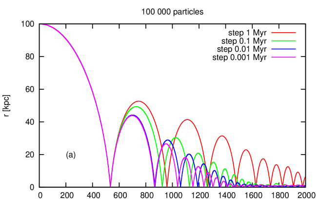
?figurename? 45: (a) Distance of the secondary from the center of the primary galaxy; (b) energy of the secondary. The motion was calculated using the MTBA with 100,000 particles for time steps of 0.001–1 Myr. Parameters of the collision are given in Sect. 19.2.

?figurename? 46: (a) Distance of the secondary from the center of the primary galaxy; (b) energy of the secondary.The motion was calculated using the MTBA with time step 0.01 Myr for 1,000-1,000,000 particles. Parameters of the collision are given in Sect. 19.2.

20 Comparison with self-consistent simulations

To compare the calculation of the dynamical friction using the methods mentioned earlier (Appendix E and Sect. 19) with the self-consistent simulations, we use the simulations performed by Kateřina Bartošková using GADGET-2. GADGET-2 is free software, distributed under the GNU General Public License. The code can be used for studies of isolated systems, or for simulations that include the cosmological expansion of space. It computes gravitational forces with a hierarchical tree algorithm (optionally in combination with a particle-mesh scheme for long-range gravitational forces) and represents fluids by means of smoothed particle hydrodynamics (SPH). Both the force computation and the time stepping are fully adaptive. The code is written in highly portable C and uses a spatial domain decomposition to map different parts of the computational domain to individual processors. GADGET-2 was publicly released in 2005 (Springel, 2005) and presently is the most widely employed code for the cosmic structure formation.

20.1 Altering GADGET-2 computational setting

The parameters of the collision have been set the same as in the previous case, Sect. 19.2, but with no cut-off diameter. $10^{5}$ particles have been used to represent the primary galaxy. The results differ for different settings of computational parameters in GADGET-2. Here we present results of five simulations that differ in settings for three chosen parameters and in the accuracy of variables during the calculation.

During the calculation of the gravitation force, spline softening is used. $SoftPar$ is the magnitude of the softening used for mutual interactions of the particles of the primary galaxy. $SoftSec$ is the softening for the secondary and in an interaction between the secondary and a particle of the primary galaxy, the larger value from $SoftPar$ and $SoftSec$ is used. $ETIA$ (ErrorTolIntAccuracy) influences the accuracy of the integration method. It is used in the estimation of the adaptive integration step $\Delta t$

$$\Delta t=\sqrt{\frac{2\,ETIA\,SoftPar}{a}},$$ (86)

where $a$ is the amount of acceleration the particle has been subjected to in the previous step. Thus the smaller $ETIA$ we choose, the shorter will be the time step. $Precision$ refers to the type of the floating-point precision used during numerical calculations.

The values we have used in the five different simulations and the labels of the simulations are shown in Table 6. The orbital decay of the satellite for all the runs is shown in Fig. 47. Run D has been calculated with the highest precision and we thus use it as a reference in the following section.

run	$ETIA$	$SoftPar$	$SoftSec$	$Precision$
		kpc	kpc
A	0.002	0.21	0.05	Single
B	0.008	0.05	0.05	Single
C	0.04	0.01	0.01	Single
D	0.04	0.01	0.01	Double
E	0.002	0.05	0.05	Single

?tablename? 6: The settings for the GADGET-2 simulations. The meaning of the parameters is explained in Sect. 20.1.

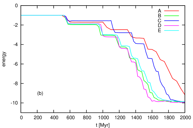
?figurename? 47: (a) Distance of the secondary from the center of the primary galaxy; (b) energy of the secondary.The motion has been calculated using GADGET-2. The parameters of the collision are given in Sect. 19.2, the settings for each simulation in Table 6.

20.2 Comparison of methods

Fig. 48 shows the orbital decay of the secondary in the merger with parameters given in Sect. 19.2 for three different methods of calculation of dynamical friction. Our modification of Chandrasekhar formula adds to the equations of motion of the secondary the dynamical friction calculated using a numerically integrated analytical formula as described in Appendix E. The MTBA method (Sect. 19) is represented by a simulation with 100,000 particles and time step of 0.01 Myr. From the self-consistent simulation with GADGET-2 we show run D (see Sect. 20.1).

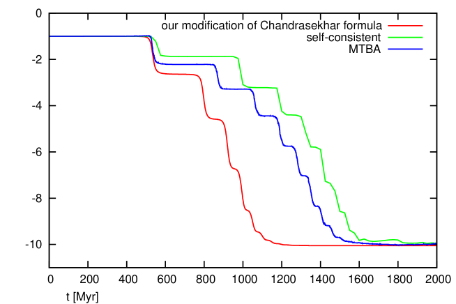
?figurename? 48: (a) Distance of the secondary from the center of the primary galaxy; (b) energy of the secondary in three different methods: our modification of Chandrasekhar formula (Sect. E.1, red curve); inconsistent simulation with GADGET-2 (Sect. 20.1, green curve); and MTBA (Sect. 19.1, blue curve). Parameters of the collision are given in Sect. 19.2.

Our modification of Chandrasekhar formula gives by far the fastest loss of the orbital energy of the satellite, but even the MTBA gives a significantly larger value of the dynamical friction than the self-consistent simulation.

In Sect. 22 we will however use our modification of Chandrasekhar formula for the calculation of the dynamical friction, as we have conducted a sizable number of simulation using this method before we became familiar with the MTBA. The MTBA is also more computationally demanding. It requires a small enough time step and the inclusion of test particles in the primary galaxy, which are otherwise of no interest for us. Our modification of Chandrasekhar formula, on the contrary, gives the same results for the motion of the secondary galaxy for the time step of 1 Myr as for any shorter step.

Doing self-consistent simulations is not an option because of the number of different simulations required for this study (most of which we do not show explicitly in this thesis). Because it seems that our modification of Chandrasekhar formula significantly overestimates the real value of the friction, the results have to be considered an upper bound for the influence of the dynamical friction on the shell structure. At the end, it turns out that the differences in the shell structure related to the choice of a method to calculate the dynamical friction is smaller than the uncertainty in the models of the tidal decay of the secondary galaxy (Sect. 21).

21 Tidal disruption

Together with the dynamical friction, the tidal disruption is another effect that is important for the galactic merger. The tidal disruption gradually lowers the mass of the cannibalized galaxy and thus mitigates the effect of the dynamical friction. During shell formation, it is of particular importance, because the gradual release of stars from the secondary galaxy has an important effect on the growing shell structure. The introduction of the tidal disruption into test-particle simulation is nevertheless a difficult task.

21.1 Massloss of the secondary

In the context of the tidal disruption of an object in the gravitation field of another body, the notion of the tidal radius is frequently introduced. This is an approximative approach to the tidal forces, assuming that under the tidal radius the matter is still bound to the disrupted body, but it is not the case anymore outside the tidal radius. The reader may find more details on the concept in Appendix F. Here we will only show how we used it in our test-particle simulations.

?figurename? 49: The purely analytical approach to the decay of the secondary galaxy during the first passage for the standard set of parameters (Sect. 17.5). Left: the evolution of the mass of the secondary galaxy. Rights: Distance of the secondary from the center of the primary galaxy (blue curve) and tidal radius of the secondary (red curve).

First we have implemented a purely analytical approach, where we calculate the current tidal radius in every step using Eq. (107) and update the mass of the secondary galaxy accordingly to the mass of a Plummer sphere with the original parameters of the secondary galaxy but restricted to the tidal radius. But this leads to us only lowering the satellite mass during the first passage through the center of the primary galaxy, see Fig. 49. Particles are released in limited amount also during further passages, but this mechanism obviously does not reflect the real situation for multiple passages.

?figurename? 50: Gradual decay of the secondary galaxy calculated using test particles. Top: distance between the centers of the primary and the secondary galaxy. Bottom: the number of particles bound to the secondary galaxy. Blue curves show the development for the simulation where we consider as bound particles those inside the sphere of the tidal radius, the red curves correspond to keeping particles with lower than escape velocity. Both simulations are carried out for the standard set of parameters (Sect. 17.5), the dynamical friction is calculated using our modification of the Chandrasekhar formula (Appendix E).

To describe the decay of the satellite during further passages, we have included in its calculation the test particles of the secondary galaxy. We count particles that we still consider bound with the satellite galaxy. The ratio between their number and the number of particles that we have put in the secondary galaxy at the beginning of the simulation determines its current mass. As a criterion for bound particles we consider that 1) the distance of the particle from the center of the secondary galaxy is lower than the current tidal radius; 2) the velocity of the particle with respect to the secondary galaxy does not exceed the escape velocity for its given distance from the center of the secondary galaxy. Fig. 50 shows how these two approaches differ for otherwise identical initial conditions.

The use of the tidal radius causes large fluctuations of the number of bound particles near the passage of the secondary galaxy through the center of the primary galaxy, when many particles suddenly find themselves outside the tidal radius. When later the secondary galaxy retreats from the center of the primary, the tidal radius quickly increases and more particles are included. Some of them eventually escape before the secondary reaches its apocenter, but still more particles stay bound to the secondary than there were during its passage through the center of the primary. In the other simulation the loss of particles is more monotonous, the orbital decay slightly faster, and more particles are caught in the center of the host galaxy.

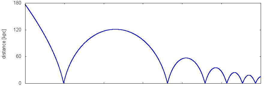
?figurename? 51: Development of the distance between the primary and the secondary galaxy (top) and the Plummer radius of the secondary galaxy (bottom). The simulations carried out for the standard set of parameters (Sect. 17.5), the dynamical friction is calculated using our modification of the Chandrasekhar formula (Appendix E). The radial density of the secondary galaxy at the beginning of the simulation and in 5 Gyr is shown Fig. 52.

The use of the two different methods to model the tidal disruption of the secondary does not have a dramatic impact on the merer. Nevertheless, the times of the passages of the secondary through the center of the host galaxy and the volume of particles released in each passage differ between the two models, mainly in the later phases of the merger. This may have a noticeable impact on the appearance of the shell system in different time, that is the positions of the shells, their number, brightness, opening angle and so forth.

The problem is that we have no hint as to which of the methods is a better approximation for the true decay of the secondary galaxy. If we were to compare the results with self-consistent simulations, we would likely get different results depending mainly on the configuration of the merger. Thus we compare the test-particle simulations done with different methods for the tidal disruption of the secondary galaxy and focus on features of the shell system that are independent of the method used (Sect. 22.1).

21.2 Deformation of the secondary galaxy

Another thing going on during the merger that is difficult to reproduce in test-particle simulations is the deformation if the cannibalized galaxy. We model components of galaxies with spherically symmetric Plummer spheres. Thus we have tried at least to change the profile of the sphere of the secondary galaxy during the simulation.

The mean value of the radial distance of a particle $\left\langle r\right\rangle$ in a Plummer sphere is given as

$$\left\langle r\right\rangle=\frac{\intop_{0}^{R_{\mathrm{tc}}}r^{\prime 3}\rho(r^{\prime})dr^{\prime}}{\intop_{0}^{R_{\mathrm{tc}}}r^{\prime\prime 2}\rho(r^{\prime\prime})dr^{\prime\prime}},$$ (87)

where $\rho(r^{\prime})$ is the density of the Plummer sphere Eq. (74) and we express the cut-off in multiplies of the Plummer radius $R_{\mathrm{tc}}=p\varepsilon$. The mean value of the radial distance is then

$$\left\langle r\right\rangle=\varepsilon\frac{2\left(1+p^{2}\right)^{3/2}-2-3p^{2}}{p^{3}}.$$ (88)

Thus if we calculate the mean value radial distance from the center of the secondary galaxy for the particles that we consider bound to it in the simulation

$$\left\langle r\right\rangle=\sum_{i=1}^{N}r_{i}/N,$$ (89)

we can easily convert it to a new Plummer radius for the secondary galaxy $\varepsilon_{\mathrm{s}}$. Fig. 51 shows the development of the Plummer radius of the secondary galaxy in a simulation with the standard set of parameters (Sect. 17.5). The Plummer radius is calculated using Eq. (88), where $\left\langle r\right\rangle$ is the mean radial distance of particles under the current tidal radius. The radial density of the secondary galaxy at the beginning of the simulation and in 5 Gyr is shown in Fig. 52. It is important to keep in mind that the density is calculated only from radial distances from the center of the satellite even though the spherical symmetry was surely broken during the simulation.

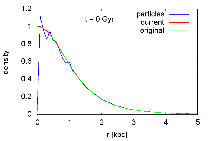
?figurename? 52: The radial density of the secondary galaxy at the beginning of the simulation and in 5 Gyr for the standard set of parameters (Sect. 17.5). In blue is the density calculated from the test particles of the secondary galaxy, in green the model of the secondary chosen at the start of the simulation and in red the density of the Plummer sphere that corresponds to the changing Plummer radius which is calculated from the distribution of the test particles. The density is normalized so that the central density of the initially chosen Plummer sphere of the secondary galaxy is one.

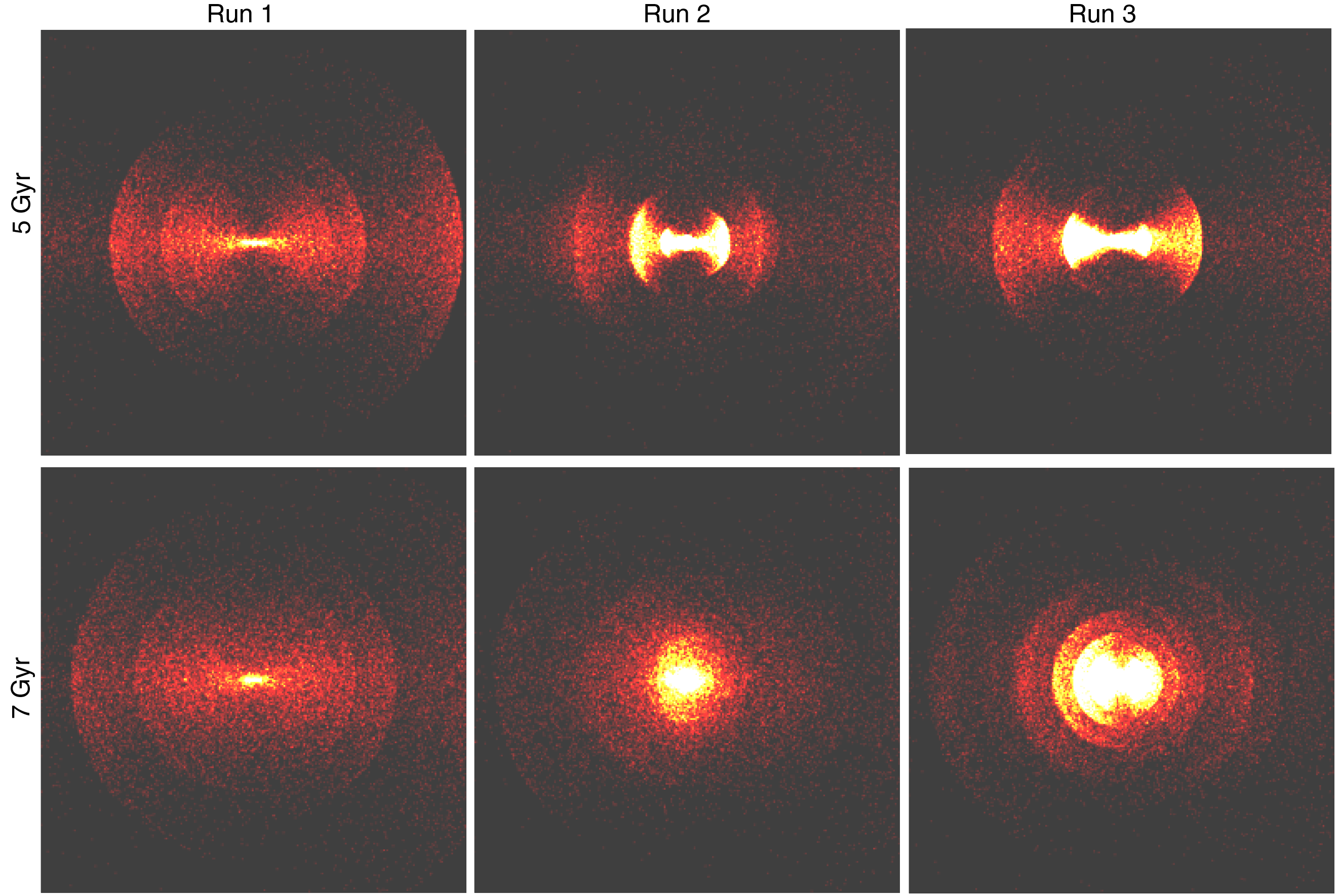
?figurename? 53: Snapshots of simulations. For description of all runs see text in Sect. 22.1. Time 0 is defined as the moment then the secondary galaxy reaches the center of the primary galaxy for the first time, which is (for all three runs) almost exactly 1 Gyr after it has been released from the distance of 180 kpc with escape velocity. Only the surface density of particles originally belonging to the satellite galaxy is displayed corresponding to the subtraction of the profile of the primary galaxy. Each box, centered on the host galaxy, shows 300$\times$300 kpc. Radial histogram of particles in 5 Gyr is shown in Fig. 54.

22 Simulations of shell structure

Now we finally show the combined effect that the inclusion of both the dynamical friction and gradual decay of the secondary galaxy in the simulations has on the shell formation. The simulations are carried out using the method described in Sect. 17, i.e. millions of test particles were generated so that they follow the distribution function of the secondary galaxy at the beginning of the simulation. The particles then move according to the sum of the gravitational potentials of both galaxies that are both represented by a smooth potential. The galaxies move with respect to each other as dictated by their masses, shape of potentials, positions and velocities.

The dynamical friction, when included, is calculated using our modification of the Chandrasekhar formula, see Appendix E, and the gradual decay of the secondary galaxy, when included, is calculated using some of the methods from Sect. 21.1. In Sect. 22.2, we have added the dark halo to the primary galaxy and Sect. 22.3 shows the shell formation in a self-consistent simulations. All the outputs are oriented so that the secondary originally approached the primary galaxy from the right hand side.

22.1 Dynamical friction and tidal disruption

We have compared three simulations, all of them for the standard set of parameters (Sect. 17.5).

• Run 1 – without dynamical friction and with instant disruption of the secondary.

• Run 2 – dynamical friction is calculated using our modification of the Chandrasekhar formula and the tidal disruption using the analytical approach based on the tidal radius as described at the beginning Sect. 21.1.

• Run 3 – dynamical friction is again calculated using our modification of the Chandrasekhar formula, the tidal disruption is based on the counting of particles inside/outside the current tidal radius. Additionally, the Plummer radius of the secondary galaxy is constantly recalculated as described in Sect. 21.2.

Snapshot from all the runs for two different times are shown in Fig. 53, radial histograms of particles in Fig. 54. Video from run 1 and run 2 is part of the electronic attachment. For the description of the video, see Appendix H point 4.

We compare a simple simulation (Run 1) with a pair of simulations (Runs 2 & 3), where the tidal decay of the secondary galaxy is modeled using two different methods. However, we can see a qualitative shift in the same direction between both Runs 2 & 3 and the simple simulation. The result of both Runs 2 & 3 is a multi-generation shell system, whereas Run 1 can in principle give rise only to one generation of shells.

For both Runs 2 & 3 there were more particles trapped in the gravitational field of the host galaxy and a large part of them has been transported to the vicinity of the center of the host galaxy. The outer shells (of the first generation) are more diffuse and significantly less luminous when compared to Run 1, whereas their positions remain essentially the same. On the other hand, in the later generations, there are brighter shells, some of which can overlap with the first-generation shells. The shells of the later generations appear on smaller radii and are often bright, whereas in Run 1 shells at small radii are completely missing. The evolution of the shell brightness in Run 1 is somehow calmer, whereas the shells of the later generations in Runs 2 & 3 have a tendency to reach very high brightness in certain small range of radii.

?figurename? 54: Radial histogram of stars of the secondary galaxy, centered on the primary 5 Gyr after the first passage of the secondary galaxy through the center of the primary galaxy for the three different simulations – run 1 (red), run 2 (green) and run 3 (blue). For description of all runs, see text in Sect. 22.1.

Runs 2 & 3 are more consistent with observations (Sect. 3) in the sense that their contain shells on both small and large radii. An important thing to notice is that within our model, any subsequent passage of the secondary galaxy through the center of the primary galaxy does not lead to a complete destruction of the shells from the previous passages. Towards the center of the host galaxy, we find shells with larger surface brightness, also a feature found in real shell galaxies. At the same time, in Runs 2 & 3 we can find faint shells surrounded by brighter ones from both sides, another effect observed in real galaxies and impossible to reproduce in a simple simulation.

The main difference between Run 2 and Run 3 lies in the positions of the shells from the later generations – those shells that dominate the system in later times thanks to their brightness. The timing of the second passage of the secondary galaxy through the center of the host galaxy is very similar for Run 2 and Run 3 but the difference in energy, mass and decay of the secondary galaxy is sufficient to produce shells at different radii. Run 3 also differs significantly from Run 2 (and also Run 1) in that a bright shells system persist even a long time after the first approach of the secondary galaxy (7 Gyr). However, we cannot say whether it is Run 2 or Run 3 that better describes the real merger of two galaxies under given initial conditions. This indicates that quantitative modeling of a shell system using test-particle simulation is very difficult or even impossible.

In spite of the difficulties, we dare to state qualitative conclusions independently on the method chosen for the tidal decay of the secondary galaxy: the introduction of the dynamical friction and the gradual decay to our simulations dramatically changes the appearance of shell structures. Only the outermost shell of the first generation is not overlayed by later, brighter generations of shells added during next passages of the satellite through the center of the primary. While the position of the outermost shell is not much affected by the dynamical friction, its brightness is rapidly lowered due to the many particles staying trapped in the weakened but remaining potential of the small galaxy.

22.2 Dark halo

To be even more realistic, we present a two-component model of the galaxy – a luminous component with a dark halo. The velocity dispersion of each component is under the influence of the other (Sect. 17.4). The velocity dispersion is an important parameter of the dynamical friction a thus values of the friction induced by each component slightly differ (the amount depends on parameters) from the values we get when the component is isolated (Sect. E.1).

We performed three simulations with parameters listed in Table 7. In all the cases, the mass of the secondary galaxy is 0.02 of the total mass of the primary; and the secondary approaches with escape velocity. Dynamical friction is calculated using our modification of the Chandrasekhar formula (Appendix E). The mass of the secondary galaxy was gradually lowered during the simulation according to the number of test particles under the current tidal radius (Sect. 21.1) and its Plummer radius was being adjusted according to the method described in Sect. 21.2.

run	$\varepsilon_{*}$	$M_{*}$	$\varepsilon_{\mathrm{DM}}$	$M_{\mathrm{DM}}$	$\varepsilon_{\mathrm{s}}$	$M_{\mathrm{s}}$	$D_{\mathrm{ini}}$	$v_{\mathrm{ini}}$
	kpc	M⊙	kpc	M⊙	kpc	M⊙	kpc	km$/$s
M0B0	7	$3.2\times 10^{11}$	-	-	2	$6.4\times 10^{9}$	180	125
M2B6	7	$3.2\times 10^{11}$	60	$6.4\times 10^{12}$	2	$1.344\times 10^{11}$	300	443
M6B10	7	$3.2\times 10^{11}$	100	$1.92\times 10^{13}$	2	$3.904\times 10^{11}$	300	756

?tablename? 7: Parameters of simulations. The potentials of the galaxies are modeled as a single Plummer sphere for the secondary galaxy in all runs and the primary galaxy in the run M0B0; and as a double Plummer sphere for the primary in runs M2B6 and M6B10. Indices *, DM and S refer to the luminous and dark components of the primary galaxy and the secondary galaxy, respectively. $\varepsilon$ is Plummer radius, $M$ total mass of the Plummer sphere, $D_{\mathrm{ini}}$ initial distance between centers of the secondary and primary galaxies and $v_{\mathrm{ini}}$ their mutual velocity.

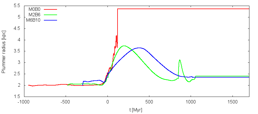
?figurename? 55: Evolution of the merger for three different configurations of the dark halo of the primary galaxy – distance between galaxies, number of particles bound to the secondary galaxy and its Plummer radius. For the parameters of the mergers, see Table 7.

?figurename? 56: Snapshots from three simulations, for the parameters of the mergers, see Table 7. Time stamps refer to the time elapsed since the first passage of the secondary galaxy through the center of the primary galaxy. Each panel covers 300$\times$300 kpc and is centered on the host galaxy. Only the surface density of particles originally belonging to the satellite galaxy is displayed. The density scale varies between frames, so that the respective range of densities is optimally covered.

Fig. 55 illustrates the evolution of the distance between the galaxies and the gradual decay of the secondary galaxy. Time stamps of each run have been shifted so that in each case the secondary galaxy reaches the center of the primary galaxy at time 0. In the first case (run M0B0 without any halo), the secondary galaxy lost all particles during the first passage and this simulation is rather equivalent to simulations with instant disruption. In the configurations that include the halo (runs M2B6 and M6B10), the velocity is such on the other hand that the primary galaxy catches only very few particles in the first passage and a significant growth of the shell structure is observed only in later phases of the merger.

Snapshots for three different times are shown in Fig. 56 and radial histograms for time 3 Gyr in Fig. 57. For the simulation with a heavy halo (run M6B10) the particles cover the largest span of energies (apocenters) and in both simulations with a halo (runs M2B6 and M6B10), new shells on lower radii are created in further passages of the secondary through the center of the primary galaxy and many particles end up being caught in the center of the primary. In the simulation without a halo (run M0B0) the secondary decays in the first passage, but the particles have mostly sizable energies at that time and thus have apocenters at larger galactocentric radii or outright escape the system. The positions of the shells in a given time are obviously different for different potentials of the primary galaxy.

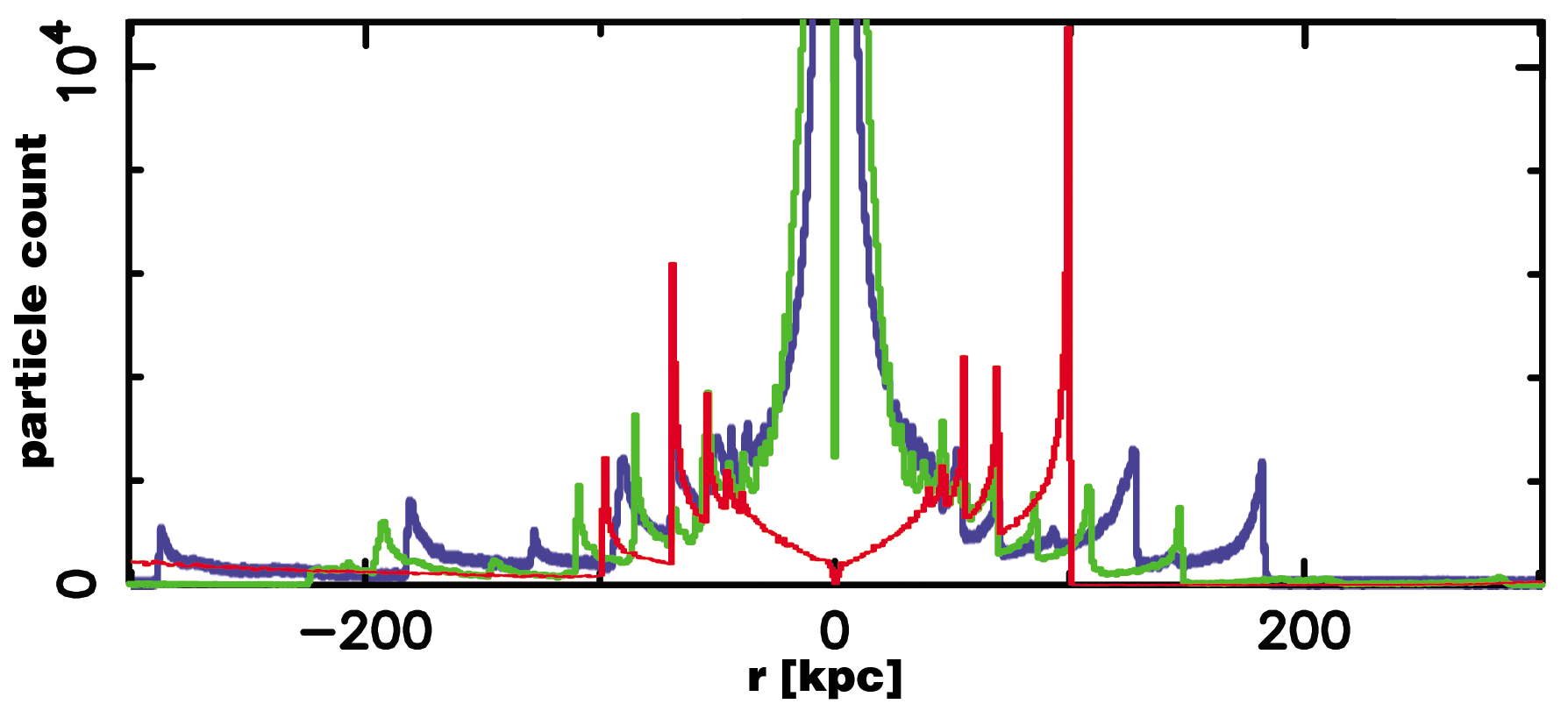
?figurename? 57: Radial histogram of stars of the secondary galaxy, centered on the primary 3 Gyr after the first passage of the secondary galaxy through the center of the primary for three different simulations. The meaning of colors is the same as in Fig. 55 (red: M0B0 – without halo, green: M2B6 – halo 20 times more massive than the luminous component, blue: M6B10 – 60 times more massive). For the parameters of the mergers, see Table 7.

The main effect of the halo on the shell system is probably in that its presence (through the increased mass of the primary galaxy) allows for a faster development of shells at larger radii, despite the secondary releasing in our case only a small part of its stars during its first passage through the center of the host galaxy. Meanwhile, there are additional shells created in the following passages, creating the high radial range of shells observed in some galaxies which has continuously proven difficult to reproduce in simulations.

The increased total mass of the host galaxy is apparently more important than the difference in the dynamical friction caused by the differences in local density and velocity dispersion for different halo configurations. The more massive halo accelerates the secondary galaxy more, reducing the loss of its energy via the dynamical friction and increasing the time before a subsequent return of the secondary galaxy. But the higher energy/velocity of the secondary galaxy allows the existence of shells at larger radii - while it is important to note that in our simulations, we see shells at 200 to 300 kpc from the center of the host galaxy, which is a distance where noone ever observed (or even looked for) shells in real galaxies.

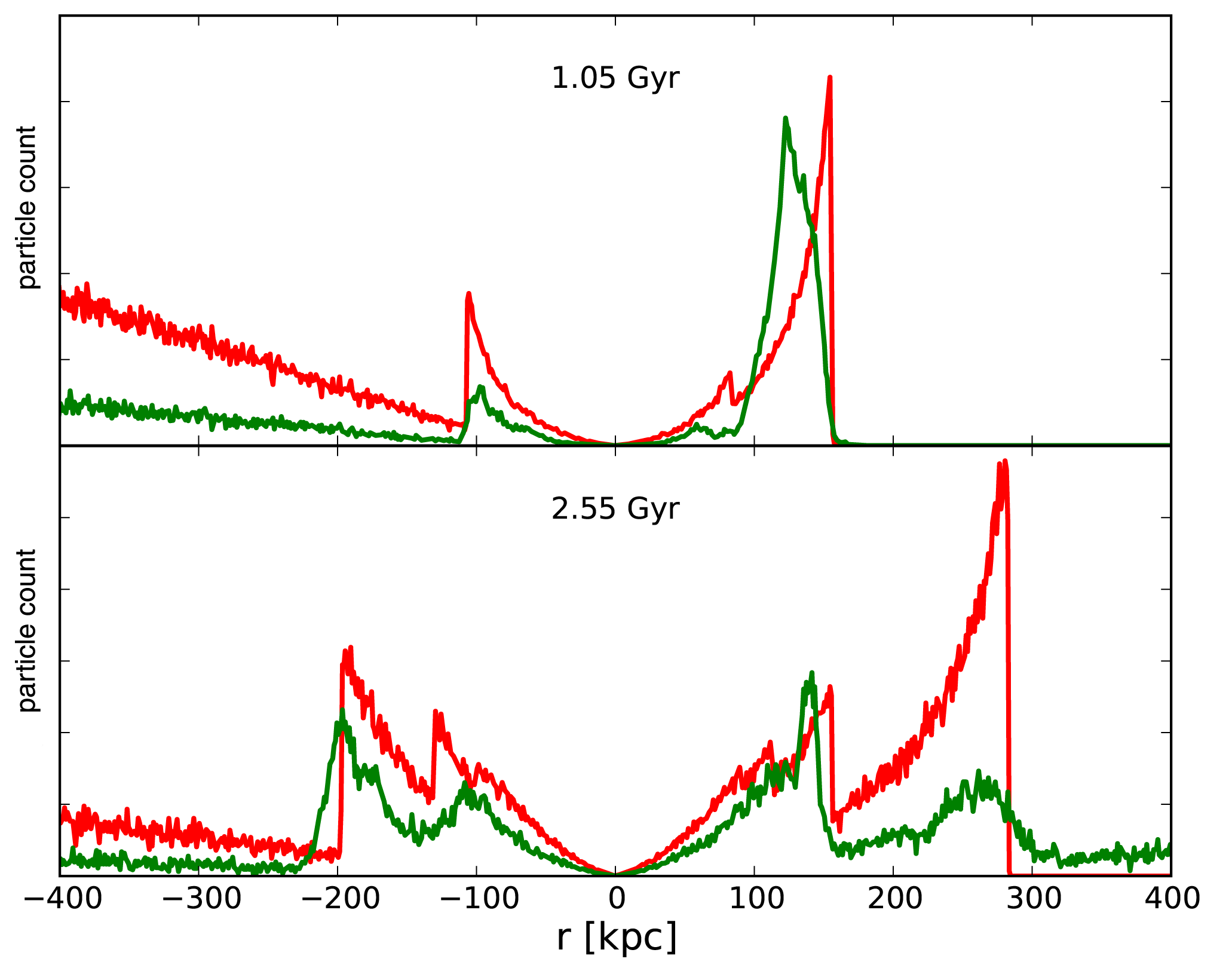
?figurename? 58: Comparison of histograms of radial distances of shells‘ particles in the self-consistent (green) and test-particle (red) simulations at two different time steps.

22.3 Self-consistent versus test-particle simulations

In this section, we compare two simulations with the same initial conditions, one conducted in a self-consistent manner using GADGET-2 by Kateřina Bartošková, the other one with test particles. Originally we intended to keep the parameters of the primary galaxy, but a two-component (luminous+dark matter) Plummer sphere is not a consistent system for an arbitrary choice of parameters, particularly for those we have used so far. The system is consistent when each physically distinct component has a positive distribution function (Ciotti, 1996). Thus we have chosen the following parameters for the merger:

The potential of the primary galaxy is a double Plummer sphere with respective masses $M_{*}=2\times 10^{11}$ M_⊙ and $M_{\mathrm{DM}}=8\times 10^{12}$ M_⊙ , and Plummer radii $\varepsilon_{*}=8$ kpc and $\varepsilon_{\mathrm{DM}}=20$ kpc for the luminous component and the dark halo, respectively. The potential of the secondary galaxy is chosen to be a single Plummer sphere with the total mass $M=2\times 10^{10}$ M_⊙ and Plummer radius $\varepsilon_{*}=2$ kpc. The cannibalized galaxy is released from the distance of 200 kpc from the center of the host galaxy with the initial velocity 102 km$/$s in the radial direction (as always).

Snapshots from several times for both of the simulations are shown in Fig. 59, radial histograms for the chosen times in Fig. 58. Video from the self-consistent simulation is part of the electronic attachment. For the description, see Appendix H point 5.

?figurename? 59: Snapshots from a test-particle simulation (left) and from the corresponding self-consistent simulation (right). Time equal zero corresponds to the passage of the secondary galaxy through the center of the primary galaxy. Each panel covers 400$\times$400 kpc and is centered on the host galaxy. Only the surface density of particles originally belonging to the satellite galaxy is displayed. The density scale varies between frames, so that the respective range of densities is optimally covered.

Unfortunately it turns out that for this choice of parameters, our method of including the gradual decay of the secondary galaxy (Sect. 21.1) does not lead to a very gradual decay at all. In the case of simulation with test particles, the secondary galaxy loses all its particles near its first passage through the center of the primary galaxy. Thus we use the model with instant disruption of the secondary instead. To make the comparison even worse, the self-consistent simulations behaves in yet another way: the core of the secondary galaxy survives the first two passages through the center of the primary galaxy and for some reason dissolves close to its apocenter.

However, despite these significant differences, the results are surprisingly similar. Most importantly, the radii of the outermost shells differ by less than 10%. In comparison with our enhanced test-particle simulations (e.g., Sect. 22.1 – Runs 2 & 3), the self-consistent simulation does not show a significant transport of particles of the secondary galaxy to the area around the center of the host galaxy, neither does it produce shells at low radii. Where on the other hand the self-consistent simulation resembles more the enhanced test-particle simulations than the simple test-particle simulation (with instantaneous disruption of the secondary galaxy and no dynamical friction) is the dramatic decrease of the brightness of the outermost shell on large radii (compare with Sect. 22.1 – Fig. 54).

23 Discussion

Our goal in this Part of the work was to include the dynamical friction and the gradual decay of the secondary galaxy in the test-particle simulations. It has been previously pointed out that coupling of these phenomena is a key effect in the shell structure formation but it was never modeled in much detail so far. Using these simulations, we aimed to asses the plausibility of timing the shell-creating merger using the outermost observed shell in a shell galaxy.

For the dynamical friction we used our own modification of the Chandrasekhar formula for radial trajectories, Appendix E, which is more faithful to the true stellar distribution function of the host galaxy. The dynamical friction calculated in this way is fully determined by the distribution function of the host galaxy and the mass and velocity of the secondary, thus is contains no free parameters. Comparison between our modification and the commonly used form of the Chandrasekhar formula, Sect. E.2, shows that the use of a constant Coulomb logarithm is completely inappropriate for radial mergers. But when compared with the self-consistent simulations, our method is found to significantly overestimate the friction, Sect. 20.2. In reality, the dynamical friction in a radial merger depends on the whole merger history and thus can be hardly reproduced by any modification of the Chandrasekhar formula, Sect. 19.1. Our simulations thus have to be understood as the upper estimate on the true effect of the dynamical friction on the shell formation.

Including the tidal disruption of the secondary galaxy in test-particle simulation is even more complicated. We have tried several methods, Sect. 21.1, and none of them is a priori better than any other. Moreover we tried to reflect on the change of the shape of the gravitational potential of the cannibalized galaxy during the merger using a variable Plummer radius, Sect. 21.2. We have carried out several simulations using different methods for the decay of the secondary galaxy, focusing on qualitative effects in which these simulations differ from simple simulations that assume instantaneous breakdown of the secondary galaxy and no dynamical friction. We can believe that effects that are independent of the method used are more likely to participate in shell forming process in reality.

One such effect is that while the position of the outermost shells of the first generation is not much affected by the inclusion of the gradual decay and dynamical friction in the simulations, its brightness is drastically lowered. The same effect is observed in our self-consistent simulation, Sect. 22.3. Even easily inferring the age of the collision is rendered impossible (as already pointed out by Dupraz and Combes, 1987). The shell systems in Fig. 54 (Sect. 22.1), all having the outermost shell at $+150$ kpc, are seen 5 Gyr after the first passage of the cannibalized galaxy through the center of the host galaxy. If we observationally identify the leftmost shell (around $-80$ kpc in Fig. 54) as being the outermost one, we would mistakenly estimate the merger age to be only $\sim 2.5$ Gyr. We would also wrongly determine the direction from which the secondary galaxy came: assuming the classical picture (based on simulations without friction and with instantaneous disruption), the outermost shell would be located on the side from which the satellite came, so we would conclude it went from the left while the opposite is true.

Furthermore, with respect to the simple simulation, in the simulations with gradual decay of the secondary, we observe the creation of new generations of shell during every passage of the remnant of the secondary galaxy through the center of the primary. In the consecutive generations, shells are created at lower radii and with higher brightness. It is important to see that, in our simulations, the subsequent passages of the secondary galaxy do not significantly disturb the existing shell structure of the previous generation and thus a shell system with a large range of radii is created. The radial range of shells observed in some real shell galaxies is truly impressive and it is impossible to reproduce in a simple simulation. It is also worth noting that in simulations with the gradual decay of the secondary, a large part of the mass of the secondary ends up in the proximity of the center of the primary galaxy.

Presence of a dark matter halo in the primary galaxy, Sect. 22.2, changes not only the dependence of the period of radial oscillations on radius (Sect. 9), but also the range of stellar energies through the change of the velocity of the accreted satellite. The halo allows for a faster development of shells at larger radii. A more massive halo creates a larger range of shell radii in our simulations than a less massive one. The increased total mass of the host galaxy is more important than the difference in the dynamical friction caused by the differences in local density and velocity dispersion for different halo configurations. The more massive halo accelerates the secondary galaxy more, reducing the loss of its energy via the dynamical friction and increasing the time before a subsequent return of the secondary galaxy. The higher velocity of the secondary galaxy also means that the primary galaxy catches only very few particles in the first passage and a significant growth of the shell structure is observed only in later phases of the merger.

In general, it seems that test-particle simulations are not suitable for a quantitative reproduction of observed shell systems. There is no reliable (semi-)analytical method to calculate the dynamical friction in radial and close-to-radial minor mergers. Apparently even more importantly, there is no universal method to model the tidal decay of the cannibalized galaxy in test-particle simulations. Unfortunately, it turns out that it is exactly the details of the decay of the secondary galaxy that affect significantly the overall shell structure. In two simulations, with apparently small differences in the loss of mass and energy of the secondary galaxy during the first passage and the time of the second passage, shells of the second generations were created at different radii with respect to the shells from the first generation (which are otherwise very similar between the simulations). Moreover, the brightness of these shells differs and with each farther passage of the secondary galaxy, the difference in the appearance of the shell system increases and the observability of shells in the host galaxy changes by whole gigayears. Overall, an accurate reproduction of a shell galaxy is a very delicate matter, as in practice we do not know an exact distribution of mass in the host galaxy, the original trajectory of the secondary galaxy, nor its own mass distribution and our simulations suggest that the shell structure is very sensitive even to small details in these quantities.

Nevertheless even despite the simplicity of the models we used, it turned out that our test-particle simulations with gradual disruption and dynamical friction of the secondary galaxy do better than the simple simulations in reproducing observed features in real shell galaxies. We thus conclude that also in real galaxies, these features are the result of combined effects of the gradual decay and dynamical friction.

At the end, we shall stress that while all these details have a large effect on the overall appearance of the shell system, they are not very important for the application of the method to measure the host galaxy potential from kinematical data that we have introduced in Part II. This method relies only on the assumption that the stars that form one particular shell are moving along radial trajectories and were released in the center of the primary galaxy together at some moment in the past. Within the framework the radial-minor-merger model, neither the gradual decay of the secondary galaxy nor the dynamical friction do not in principle have a large influence on the radiality of the stellar trajectories. Also, even when these effects are present, stars are being released in short time intervals when the secondary galaxy passes through the center of the primary galaxy, however these intervals are slightly larger than zero, which would be the case for the instantaneous decay of the secondary galaxy. This fact causes the shells to be slightly more diffuse and can interfere with an effort to determine the positions of the spectral peaks and the shell edge. Nevertheless, in principle the measurement of the potential should be still possible.

?partname? IV Conclusions

In Part I we have summarized observational and theoretical knowledge about the shell galaxies according to the available literature. Shell galaxies are mostly elliptical galaxies containing fine structures which are made of stars and form open, concentric arcs that do not cross each other. The most prominent observational characteristics of shells are summarized in 22 points in Sect. 4. In Sect. 5, we introduce all proposed scenarios of origin of shell galaxies. The most widely accepted theory, supported by a multitude of observational evidence, is the close-to-radial minor merger of galaxies introduced by Quinn (1984). In the framework of this model, Merrifield and Kuijken (1998) suggested using shell kinematics to measure the potential of the host galaxy. The issue of the determination of the overall potential and distribution of the dark matter in galaxies is among the most prominent in galactic astrophysics since the most successful theory of the evolution of the Universe so far seems to be the theory of the hierarchical formation based on the assumption of the existence of cold dark matter, significantly dominating the baryonic one. Thus, independent measurement of the dark matter content in galaxies is highly desirable. Measurement of galactic potential is particularly difficult in elliptical galaxies at large distances from the center of the galaxy. Incidentally, shells are found mainly in elliptical galaxies and they do occur in distances up to 100 kpc from the center.

The method of Merrifield and Kuijken (1998) is based on the approximation of a stationary shell. Using positions of peaks in the line-of-sight velocity distribution (LOSVD), it allows the calculation of the gradient of the potential near the shell edge. We have developed this method further in Part II assuming validity of the radial-minor-merger model and spherical symmetry of the host galaxy. Using both analytical calculations and test-particle simulations, we have shown that the LOSVD has a quadruple shape in this situation. Assuming a constant shell phase velocity and a constant radial acceleration in the host galaxy potential for each shell, we have developed three different analytical and semi-analytical approaches (Sect. 11.6) for obtaining the circular velocity in the host galaxy and the current shell phase velocity from the positions of the peaks of the maxima of the LOSVD.

The applicability of our different approaches varies with the character of measured data. As obtaining suitable data is at the very limit of current observational tools and thus no such data is yet available for analysis, we have applied our methods to results of a simulation of a radial minor merger. We were able to reproduce the circular velocity at shell radii to within $\sim 1$ % from the actual value. Applying the method of Merrifield and Kuijken (1998) to the simulated data, we have derived a circular velocity larger by 40–50% than the true value.

All our approaches, however, derive the shell phase velocity systematically larger, 7–30%, than the real velocity is. That can be caused by nonradial trajectories of the stars of the cannibalized galaxy or by poor definition of the shell radius in the simulation. The method of Merrifield and Kuijken (1998) does not allow to derive the shell phase velocity at all since it is based on the approximation of a stationary shell.

In the case of spherical symmetry, the value of the circular velocity directly determines the amount of mass enclosed under the given radius, thus determining the dark matter content of the galaxy. On the other hand, the shell velocity depends on the serial number of the shell and on the whole potential from the center of the galaxy up to the shell radius and thus its interpretation is less straightforward. A comparison of its measured velocity to theoretical predictions is possible only for a given model of the potential of the host galaxy and the presumed serial number of the observed shells. In such a case, however, it can be used to exclude some parameters or models of the potential that would otherwise fit the observed circular velocity. Moreover, the measurement of shell velocities can theoretically decide whether the outermost observed shell is the first one created; determine the time from the merger and the impact direction of the cannibalized galaxy; and reveal the shells from different generations, which can be present in a shell galaxy (Bartošková et al., 2011).

In Part II we have examined effects of the gradual decay and dynamical friction of the cannibalized (secondary) galaxy on the appearance of the shell structure. Our goal was to asses the plausibility of timing the shell-creating merger using the outermost observed shell in a shell galaxy. Attempts to date a merger from observed positions of shells, using simple test-particle simulations, have been made in previous work of Canalizo et al. (2007) supporting a potential causal connection between the merger, the post-starburst ages in nuclear stellar populations, and the quasar.

We have searched for a method to include the gradual decay and dynamical friction of the secondary galaxy into the test-particle simulations. While these effects are (along with many other physical processes) naturally included in self-consistent simulations, using these has also some serious drawbacks when compared to test-particle simulations. For example, some effects seen in self-consistent simulations are difficult or outright impossible to reproduce by analytical or semi-analytical methods. At the same time, their manifestation in self-consistent simulations is difficult to separate and sometimes they may even be confused with non-physical outcomes of used methods. Moreover, self-consistent simulations with high resolution necessary to analyze delicate tidal structures such as the shells are demanding on computation time. This demand is even larger if we want to explore a significant part of the parameter space.

For the dynamical friction we used our own modification of the Chandrasekhar formula for radial trajectories, Appendix E. The dynamical friction calculated in this way is fully determined by the distribution function of the host galaxy and the mass and velocity of the secondary, thus is contains no free parameters. But when compared with the self-consistent simulations, our method is found to significantly overestimate the friction, Sect. 20.2. Our simulations thus have to be understood as the upper estimate on the true effect of the dynamical friction on the shell formation.

We have tried several methods for including the tidal disruption and deformation of the secondary galaxy, Sect. 21, and none of them is a priori better than any other. In our simulations it turns out that the resulting shell system is very sensitive to small differences during the decay of the cannibalized galaxy and thus the test-particle simulations are not suitable for a quantitative reproduction of observed shell systems. We have thus focused on qualitative effects in which our enhanced simulations differ from simple simulations that assume instantaneous breakdown of the secondary galaxy and no dynamical friction. It turned out that these enhanced test-particle simulations do better than the simple simulations in reproducing observed features in real galaxies, including features that the simple simulations cannot show at all. We thus conclude that also in real galaxies, these features are the result of combined effects of the gradual decay and dynamical friction.

One effect found commonly in all the enhanced test-particle simulations is that while the position of the outermost shells of the first generation is not much affected by the inclusion of the gradual decay and dynamical friction in the simulations, its brightness is drastically lowered. The same effect is observed in our self-consistent simulation, Sect. 22.3. Even just inferring the age of the collision is thus tricky: if we observationally miss the weakened outermost shell, which should be clearly visible according to simple simulations, we would underestimate the merger age by a factor of 2. At the same time, we would also wrongly determine the direction from which the secondary galaxy came.

Ideally, for systems with multiple shells we would like to combine measurements of shell kinematics and their radial distribution, possibly also with measurements of surface brightness profile (Sect. 14.4). The kinematical measurements supply us with the magnitude of acceleration at the shell edge and an estimate of the phase shell velocity, which allows us to separate the shells in different generations, if these are present. Simulations with the dynamical friction and gradual decay of the secondary galaxies that reproduce the kinematic and photometric data will then constrain other parameters of the merger such as its age and the trajectory and nature of the satellite galaxy. A similar result has been obtained for M31, Fardal et al. (2007, 2008, 2012), whereas for the other shell galaxies, obtaining the kinematical data is a great challenge for the next generation of astronomical instruments.

?partname? V Appendix

?appendixname? A Units and conversions

When dealing with galaxies, we need to describe objects and time spans incommensurable with our daily experience that defines the standard sets of units, such as SI. Throughout the text we thus use a set of units adapted for this task – we measure the mass in M_⊙ the length in kpc and the time in Myr. Although their meaning is clear, they sometimes give rise to rather awkward derived units. We will briefly list the most prominent of them (together with the basic ones) and give their relation to the SI and cgs units.

• 1 Myr = $10^{6}$ yr = $3.156\times 10^{13}$ s

• 1 kpc = 3 262 ly = $3.086\times 10^{19}$ m = $3.086\times 10^{21}$ cm

• 1 M_⊙ = $1.989\times 10^{30}$ kg = $1.989\times 10^{33}$ g

• 1 kpc$/$Myr = 977.8 km$/$s = $9.778\times 10^{7}$ cm$/$s (the roundness of this value allows for an easy conversion for most of our plots)

• 1 kpc$/$Myr²= $3.098\times 10^{-8}$ m$/$s² = $3.098\times 10^{-6}$ cm$/$s²

• 1 M_⊙$/$kpc³= $6.768\times 10^{-29}$ kg$/$m³ = $6.768\times 10^{-32}$ g$/$cm³

• 1 kpc³$/$Myr²$/$M_⊙ = 14.83 m³$/$s²$/$kg = 14 830 cm³$/$s²$/$g –
  thus G = $6.674\times 10^{-11}$ m³$/$s²$/$kg = $4.500\times 10^{-12}$ kpc³$/$Myr²$/$M_⊙

?appendixname? B List of abbreviations

AU

arbitrary unit, a relative placeholder unit for when the actual value of a measurement is unknown or unimportant

DM

dark matter

FWHM

full width at half maximum, parameter of Gaussian function

GADGET-2

free software used for self-consistent simulations, see Sect. 20

KDC

kinematically distinct/decoupled cores of galaxies, see Sect. 3.7

LOS

line-of-sight

LOSVD

line-of-sight velocity distribution

MK98

paper about measuring gravitational potential using shell kinematics Merrifield and Kuijken (1998)

MTBA

Multiple Three-Body Algorithm, a method used by Seguin and Dupraz (1994) to study dynamical friction in head-on galaxy collisions, see Sect. 19

S$/$N

signal-to-noise ratio

WIM

Weak Interaction Model of origin of shell galaxies by Thomson and Wright (1990), see Sect. 5.2

?appendixname? C Initial velocity distribution

The shell-edge density distribution, $\sigma_{\mathrm{sph}}\left(r_{\mathbf{s}}\right)$, is defined by Eq. (13). Note that, since, in the model of the radial oscillations, all stars at the shell edge have the same energy, the function $N\left(r_{\mathbf{s}}\right)$ determines the distribution of stellar apocenters, the radial dependence of which differs just slightly from $\sigma_{\mathrm{sph}}\left(r_{\mathbf{s}}\right)$.

Let $f(r_{\mathrm{ac}})$ and $g(v_{0})$ be the distribution function of the stellar apocenters and the initial velocities, respectively, then

$$g(v_{0})=f(r_{\mathrm{ac}})\frac{\mathrm{d}r_{\mathrm{ac}}}{\mathrm{d}v_{0}}.$$ (90)

In almost all cases in the thesis $\sigma_{\mathrm{sph}}\left(r_{\mathbf{s}}\right)\propto 1/r_{\mathbf{s}}^{2}$, so the distribution function of the stellar apocenters is a constant function $f(r_{\mathrm{ac}})=A$.

Initially, all stars are at the center of the host galaxy, so

$$v_{0}=\sqrt{-2\left[\phi(r_{\mathrm{ac}})-\phi(0)\right]},$$ (91)

where $\phi(r)$ is the spherically symmetric potential of the host galaxy. Then

$$g(v_{0})=A\left.\frac{\mathrm{d}\phi(v)}{\mathrm{d}v}\right|_{v=v_{0}}v_{0},$$ (92)

where $\phi(v)$ is inverse function to $v_{0}\left(\phi\right)$ given by Eq. (91).

The correspondence between the shell-edge density distribution and initial velocity distribution is one-to-one, unlike for example the one between the spatial (or projected) density and the shell-edge density distribution, Eq. (14), as the density at one radius receives contributions from particles with two distinct velocities.

?appendixname? D Introduction to dynamical friction

Appendix D was, with some adjustments, adapted from the master thesis Ebrová (2007).

D.1 A thermodynamic meditation

The dynamical friction is a braking force of gravitational origin, caused by the sole fact that the area, through which the secondary galaxy (or, in general, any object passing through a galaxy or another extended object) flies is not an empty space filled with a smooth potential, but a large sea of individual stars.

Thinking deeper, we can easily see that some slowdown of the secondary galaxy is inevitable. Every system, where energy transfer is possible tends to temperature equilibrium. In a system of at least three gravitating bodies such a transfer is indeed possible and frequently happens. The relatively fast and heavy secondary galaxy possesses a decent amount of kinetic energy and as such it is just a hot piece thrown into a colder sea of the stars of the primary galaxy. The slowdown of the intruder that cannot be accounted for in the fixed-potential model, is the way of leveling the temperatures. The kinetic energy transfers to the primary’s stars – the same effect causes the heating of the cold disk population in the week interaction model, as mentioned in Sect. 5.2.

The reality of this process can be grasped from a different point of view. The relatively massive secondary galaxy attracts the primary’s stars and thus creates an area of a higher density of stars behind itself. The passing galaxy is attracted backwards by this condensation, lowering its speed towards the primary.

D.2 Chandrasekhar formula

An analytical derivation of such a braking force is based on the following thought: In a distant encounter with just one star, the velocity of an object cannot be changed, instead it is only deflected from the original direction and thus enriched with a component of speed perpendicular to the original direction. For a very massive body, as our secondary galaxy is, the magnitude of this perpendicular component will not be large, neither will be the loss of the velocity in the original direction. But when it undergoes many such encounters, the contributions add. The contributions in the perpendicular directions will have randomly scattered azimuthal angles and thus add to zero (except for the overall action of the smooth potential). On the other hand, the contributions to the original direction of the velocity will always be opposite to it, resulting in the braking of the galaxy.

The Chandrasekhar formula was originally derived by Chandrasekhar (1943). Here we present a short version of the presentation of the chapter 7.1 in the bible of the galactic astronomy, “Galactic Dynamics” by Binney and Tremaine (1987).

To start, let us imagine the encounter of our object of interest with a single star. When two bodies meet, energy is not transferred, but the direction of velocity of our object changes. It is a matter of a simple mechanics and as a result, the change of the component of velocity parallel to its original direction, $\mid\mathbf{\bigtriangleup v}_{M\parallel}\mid$ between the times $t=-\infty$ and $t=\infty$ is given by (Eq. 7-10b in Binney and Tremaine, 1987; see its derivation there):

$$\mid\bigtriangleup\mathbf{v}_{M\parallel}\mid=\frac{2\,m\,V_{0}}{M+m}\left[1+\frac{b^{2}V_{0}^{4}}{G^{2}(M+m)^{2}}\right]^{-1},$$ (93)

where $M$ is our object’s (the secondary galaxy) mass, $m$ is the mass of the star, $b$ the impact parameter (the length of $\mathbf{b}$, the vector indicating the position of the star in a plane perpendicular to the original velocity of the galaxy) and $\mathbf{V}_{0}$ is the difference between the original velocity of the star $\mathbf{v}_{m}$ and velocity of our object $\mathbf{v}_{M}$, so $\mathbf{V}_{0}=\mathbf{v}_{m}-\mathbf{v}_{M}$. The bold typeface indicates vectors, and their length is indicated by the same symbol in normal type.

For an object flying through a field of stars with the phase-space number density of stars $f(\mathbf{v}_{m},\mathbf{b})$, the change in the parallel component of velocity $\mathrm{d}\mathbf{v}_{M\parallel}$ in an infinitesimal time $\mathbf{\mathrm{d}}t$ will be given by the integration of Eq. (93) multiplied by the density $f(\mathbf{v}_{m},\mathbf{b})$ over the plane of $\mathbf{b}$ and the space $\mathbf{v}_{m}$. For $\mathbf{b}$ is measured from a given point in a plane, it is advantageous to use the polar coordinates $(b,\varphi)$:

$$\frac{\mathrm{d}\mathbf{v}_{M\parallel}}{\mathrm{d}t}=\intop\intop\intop f(\mathbf{v}_{m},b,\varphi)\frac{2m\,V_{0}(\mathbf{v}_{m})\,\mathbf{V}_{0}(\mathbf{v}_{m})}{(M+m)\left[1+\frac{b^{2}V_{0}^{4}(\mathbf{v}_{m})}{G^{2}(M+m)^{2}}\right]}\mathrm{d}^{3}\mathbf{v}_{m}\,b\mathrm{d}b\,\mathrm{d}\varphi.$$ (94)

To derive the Chandrasekhar formula we further assume the homogeneity of the field of stars, so as the distribution function of the stars does not depend on $\mathbf{b}$. The remaining $\mathbf{b}$-dependent part is of the following form a can be easily integrated from 0 to some $b_{\mathrm{max}}$:

$$\intop_{0}^{b_{\mathrm{max}}}\frac{b\mathrm{d}b}{1+c^{2}b^{2}}=\left[\frac{\ln(1+c^{2}b^{2})}{2\,c^{2}}\right]_{b=0}^{b=b_{\mathrm{max}}},$$ (95)

where in our case $c=V_{0}^{2}/[G(M+m)]$. It is conventional to introduce the notation

$$\Lambda=\frac{b_{\mathrm{max}}V_{0}^{2}}{G(M+m)}.$$ (96)

A typical value of $\Lambda$ would be of the order of $10^{3}$, thus we can neglect the one and put $\frac{1}{2}\ln(1+\Lambda^{2})\cong\ln(\Lambda)$. This factor is often called the Coulomb logarithm. Furthermore we assume that we do not err too much when replacing $V_{0}$ in $\Lambda$ by $v_{\mathrm{typ}}$, a typical speed. Then the Coulomb logarithm does not depend on $\mathbf{v}_{m}$, and still $V_{0}=\mid\mathbf{v}_{m}-\mathbf{v}_{M}\mid$ and the whole Eq. (94) goes to

$$\frac{\mathrm{d}\mathbf{v}_{M\parallel}}{\mathrm{d}t}=4\pi\ln(\Lambda)G^{2}m(M+m)\intop f(\mathbf{v}_{m})\frac{\mathbf{v}_{m}-\mathbf{v}_{M}}{\mid\mathbf{v}_{m}-\mathbf{v}_{M}\mid^{3}}\mathrm{d}^{3}\mathbf{v}_{m}.$$ (97)

The integral is of exactly the same form as in the Newton’s law of gravity and if the stars move isotropically, the density distribution is spherical and by Newton‘s first theorem (see Binney and Tremaine, 1987; chapter 2), the total acceleration of our object by dynamical friction is:

$$\frac{\mathrm{d}\mathbf{v}_{M\parallel}}{\mathrm{d}t}=-16\pi^{2}\ln(\Lambda)G^{2}m(M+m)\frac{\intop_{0}^{v_{M}}f(v_{m})v_{m}\mathrm{d}v_{m}}{v_{M}^{3}}\mathbf{v}_{M}$$ (98)

i.e., only stars moving slower then our object contribute to the force and this force always opposes the motion. Eq. (98) is usually called the Chandrasekhar dynamical friction formula.

If $f(v_{m})$ is Maxwellian with dispersion $\sigma$

$$f=\frac{n_{0}}{(2\pi\sigma^{2})^{3/2}}\exp(-\frac{1}{2}v^{2}/\sigma^{2}),$$ (99)

we can integrate Eq. (98). The density of the stars is $\rho_{0}=n_{0}\,m$ and for $M\gg m$, what happens to be our case, we can put $(M+m)\cong M$, and then Eq. (98) reads:

$$\frac{\mathrm{d}\mathbf{v}_{M\parallel}}{\mathrm{d}t}=-\frac{4\pi\ln(\Lambda)G^{2}\rho_{0}M}{v_{M}^{3}}\left[\mathrm{erf}(X)-\frac{2\,X}{\sqrt{\pi}}\mathrm{e}^{-X^{2}}\right]\mathbf{v}_{M},$$ (100)

where $\Lambda$ is given by Eq. (96), $X\equiv v_{M}/(\sigma\sqrt{2})$ and erf($X$) is the error function given by

$$\mathrm{erf}(X)\equiv\frac{2}{\sqrt{\pi}}\intop_{0}^{X}\mathrm{e}^{-t^{2}}\mathrm{d}t$$ (101)

for which we can obtain tabulated values, or we can pre-generate them numerically with an arbitrary precision.

D.3 What a wonderful universe

Giving it a deeper thought, one can consider the validity of the Chandrasekhar formula almost a miracle. We have by the way disclosed that it works, at least approximately – the confrontation with numerical simulations of flybys through a galaxy or a cluster has been carried out by e.g. Lin and Tremaine (1983); Bontekoe and van Albada (1987), who proved that the analytical solution (given by the Chandrasekhar formula) is in a good agreement with the simulations in a relatively wide range of situations. The analytical solutions has some freedom in the Coulomb logarithm which is not completely well-defined. Its correct choice can help to better reproduce the numerical results and compensate other drawbacks of the formula – anyway, the freedom is small when we demand the Coulomb logarithm to stay constant.

?figurename? 60: The path and velocity changes of the objects undergoing encounters with individual stars. The absolute value of the velocity remains unchanged.

But back to our astonishment. When the secondary galaxy deviates from its course, its speed in the original direction is reduced. But after meeting another star that compensates the deviation, it also gets back the original velocity in this direction, as is shown in Fig. 60.

The point is that the Chandrasekhar formula evaluates the change of the parallel component of the velocity after the flyby from infinity to infinity for every single star with the same initial conditions and then adds these changes and applies them to the secondary galaxy in one moment, the moment of the closest approach with these stars, see Fig. 61. The change of the parallel component of the velocity and the compensation of the changes in the perpendicular direction then happen somehow at the same time, although the magnitude of their effect is calculated as if they happen consecutively – and by some wonder, it works.

?figurename? 61: A schematic depiction of the change of the velocity of the secondary galaxy after three steps. In every moment, only the influence of the stars lying in one plane perpendicular to the motion of the galaxy is taken into account.

Let us just remark that the fact that we account for the influence of the stars in the moment of the closest approach is not so strong neglection. During an encounter of two bodies, roughly one half of the velocity change takes place around the point of the closest approach on the scale of the impact parameter. For the encounter of the galaxy with two stars, it is confirmed in the right panel of Fig. 62.

D.4 Why does it work?

We can see the mechanism of the dynamical friction in action even in a simple model of a “galaxy” interacting with two “stars”, results of which are seen in Fig. 62. Although the model is a very simple one, it allows us to see in practice that yet in the system of three bodies (in contrary to two) the permanent energy and momentum transfer is possible. The symmetry of the configuration ensures that the galaxy will keep a straight line and thus any change of velocity it undergoes will be a change in the magnitude of the velocity. According to the idea of an infinite sea of stars, we take into account only the interaction between the stars and the galaxy, not mutually between the stars.

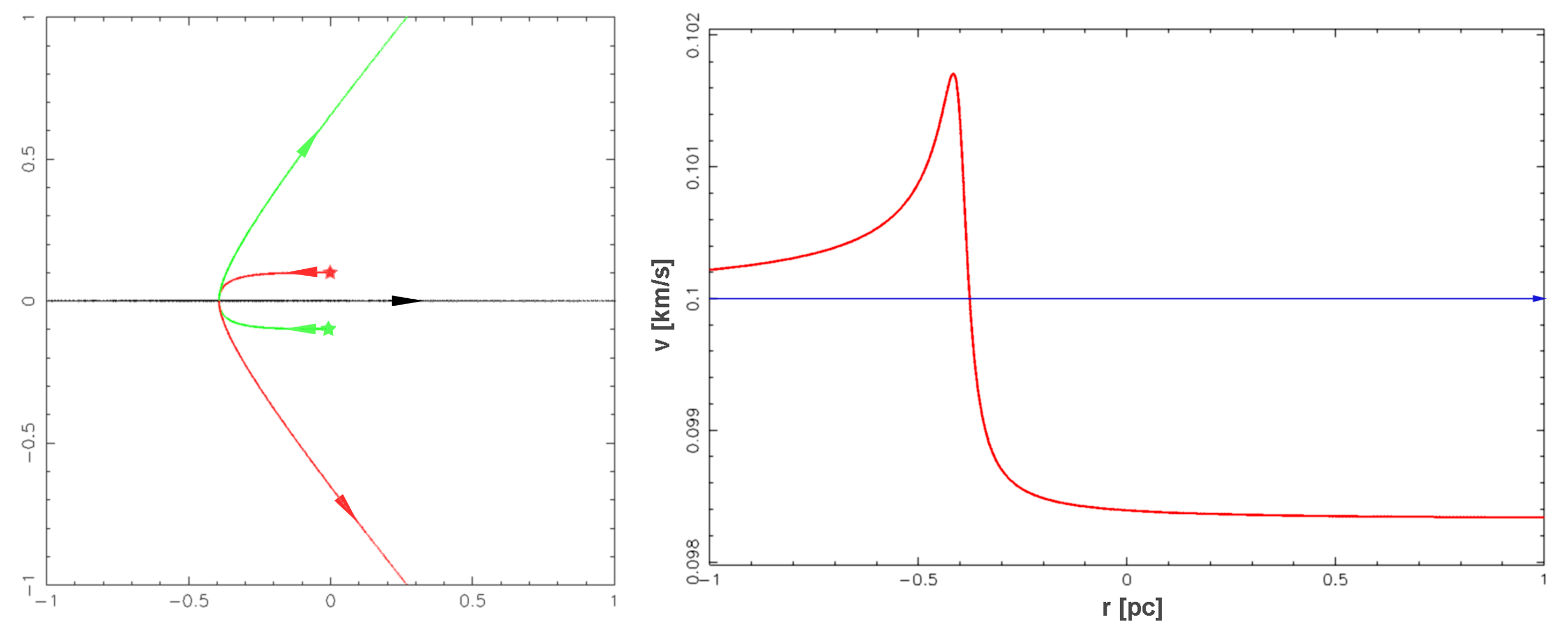
?figurename? 62: The result of the simulation. A large body (with the mass of 200 M_⊙, straight black line) moves in the direction of the $x$-axis (with the velocity of only 100 m$/$s – this and the other unrealistic values have been chosen only to make the picture more illustrative in a linear and uniform scale) and encounters a pair of stars (2 M_⊙ each) that are initially place symmetrically with respect to its track (0.1 pc from the track). The mutual gravitational attraction of the stars is neglected. The right panel shows the development of the velocity of the large body during the closest approach. The blue line represents its original velocity, thus its path if the stars were not present.

It is clear that due to the galaxy’s gravity, the stars begin to move towards its track (meanwhile also moving towards the galaxy along the track, but let us not care for a moment). While the stars move towards the track, the attraction accumulates and they gather speed. When they cross the galaxy’s track, the galaxy starts pulling them back (at least when we speak about the perpendicular component of the velocity) and they slow down. Anyway, thanks to the fact that they cross the track after the galaxy’s passage, they spend more time in the phase where their perpendicular velocity component is increased than otherwise and finally they retain some speed in this direction. But it means they have gathered kinetic energy, what must be at the expense of the galaxy’s kinetic energy and so the speed of the galaxy must have decreased (that is the dynamical friction) – even though it has moved much faster than before during the closest approach of the encounter. In reality, the situation is a little more complex, because apart from the energy, the momentum has to be also conserved – the momentum of the galaxy has decreased and so the stars must have also a non-zero parallel component of the velocity, to maintain this component of momentum.

In accordance with the derivation of the Chandrasekhar formula, we use Eq. (93) just multiplied by two to derive the analytical formula for the change of the galaxy’s velocity. For the impact parameter $b$ we obviously put the original distance between the stars and the galaxy’s track. Our numerical tests for various values of parameters (masses, initial velocity of the galaxy, impact parameter) show that the analytical results obtained this way tend to overestimate the decrease in the velocity, typically by about 15 per cent.

It could be anticipated that the numerical and analytical results will differ, as the analytical formula counts with two separated encounters from infinity to infinity. In such a case the galaxy follows a curved trajectory and thus its interaction with the star is slightly different than when both encounters happen at the same time and the galaxy is forced to stay on a straight line. Let us remark that we have tested the model by removing one of the stars and then the results for the change of the parallel component of the velocity differ from the prediction in fractions of per mille.

In reality, the situation is even more complex, there are many stars in the game and they also mutually interact and undergo the influence of all the surrounding stars that do not take part in the dynamical friction directly.

?appendixname? E Our method

In Ebrová (2007) we have introduced our method to calculate the dynamical friction in restricted $N$-body simulations during the radial merger. In this section we remind the reader of its characteristics and derivation as introduced in the master thesis.

E.1 Avoiding some approximations

The Chandrasekhar formula contains two kinds of inaccuracies. The first of them is the principal one, namely the fact that the change in the parallel component of the velocity from any individual star is added instantaneously at the point of the closest approach (of the secondary galaxy) to it. We have already shown that it is not too wrong, but what is worse, the influence of the star is taken to be such as if the galaxy passed it from infinity to infinity and there was nothing in the universe but the star and the galaxy. Sects. D.2–D.4 for details.

The second source of inaccuracy lies in all the approximation that have been done when passing from Eq. (94) to Eq. (98). These will concern us in this section, leaving aside the assumptions of the Maxwellian velocity distribution and the negligence of the masses of the stars compared to that of the secondary galaxy, that led us from Eq. (98) to Eq. (100), which we use in the simulations and keeping the “principal inaccuracy” mentioned above.

The first approximations that allowed us to integrate Eq. (94) over the plane of the impact parameter was the assumed homogeneity of the star field, i.e. that the distribution function does not depend on position. Then we have taken the Coulomb logarithm to be independent of velocity of the stars $\mathbf{v}_{m}$ (it obviously isn’t, but it varies slowly) and this has allowed us to simplify the $\mathbf{v}_{m}$-integral and given a suitable choice of the distribution function we could even carry out the integration (see Sect. D.2). Both steps are only approximate even in the simple case of the spherical galaxy with the Plummer profile, as both the density – Eq. (74) and the velocity dispersion – Eq. (80) of the Plummer sphere do depend on the radius.

If we wish to avoid these simplification, we have to turn back to Eq. (94) and put in e.g. the Maxwellian distribution, Eq. (99), for $f(\mathbf{v}_{m},b,\varphi)$, together with putting $n_{0}m=\rho$, where $\rho$ is the density of the primary at a given point – keeping in mind that the radius $r$ (the distance of a point from the center of the primary galaxy) on which the formulae depend is a function of $b$, $\varphi$ and in fact also of the direction of motion of the braked body (the secondary galaxy). When dealing with the radial mergers, this direction points towards the center of the primary galaxy and $r$ becomes a particularly simple function of $b$:

$$r=\sqrt{d^{2}+b^{2}},$$ (102)

where $d$ is (also in the following) the distance between the centers of the primary and the secondary galaxy. There is no $\varphi$-dependence in the radial case and the integration gives a trivial factor of $2\pi$. For simplicity, we put the Eq. (80) for the velocity dispersion, as the friction is essentially negligible for both the simple and the cut-off dispersion in the areas where they significantly differ (see Fig. 43). Furthermore, during the multiple passages that occur in the simulations (where the friction becomes significant) the secondary galaxy does not reach these areas at all. Using Eq. (80) for the cut-off velocity dispersion would thus unnecessarily complicate the already complex formulae.

Putting all this together, we get

$$\frac{\mathrm{d}\mathbf{v}_{M\parallel}}{\mathrm{d}t} = \frac{3^{5/2}\varepsilon_{\mathrm{p}}^{2}}{(\pi G)^{3/2}M_{\mathrm{p}}^{1/2}M_{\mathrm{s}}}\intop\intop\frac{\mid\mathbf{v}_{m}-\mathbf{v}_{M}\mid(\mathbf{v}_{m}-\mathbf{v}_{M})}{(b^{2}+d^{2}+\varepsilon_{\mathrm{p}}^{2})^{7/4}}\times$$ (103)

$$\times\left[1+\frac{b^{2}(\mathbf{v}_{m}-\mathbf{v}_{M})^{4}}{G^{2}M_{\mathrm{s}}^{2}}\right]^{-1}\mathrm{\exp\left[-\frac{3\mathbf{v}_{\mathit{m}}}{\mathit{GM_{\mathrm{p}}}}\sqrt{\mathit{b}^{2}+\mathit{d}^{2}+\varepsilon_{\mathrm{p}}^{2}}\right]}b\mathrm{d}b\,\mathbf{\mathrm{d^{3}}v}_{m},$$

where the meaning of the variables is the same as when we derived the Chandrasekhar formula in Sect. D.2. The indexes $p$ and $s$ again stand for the parameters of the primary and the secondary galaxy, respectively.

First, we shift the integration variable to $\mathbf{v}_{m}^{\prime}=\mathbf{v}_{m}-\mathbf{v}_{M}$ and immediately rename it back $\mathbf{v}_{m}^{\prime}\rightarrow\mathbf{v}_{m}$. We then perform the scalar product with the unit vector $\mathbf{v}_{M}/v_{M}$ on both sides, getting the projection of the friction acceleration to the direction of the velocity of the secondary galaxy. This is by symmetry its only nonzero component in the radial case and it will be advantageous to deal with a scalar-valued integral. The negative value means that the friction acts in the direction opposite to the motion of the braked body, what is the only feasible situation in any setup with an isotropic velocity distribution in the primary galaxy.

Transforming to the spherical coordinates (taking the $z$-axis parallel with the velocity of the secondary galaxy), we have $\mathbf{v}_{m}\cdot\mathbf{v}_{M}=v_{m}v_{M}\cos\theta$ and again no dependence on the azimuthal angle, leaving us with the obligatory factor of $2\pi$. The $\theta$-integral then can be carried out in the form that could be with some effort put on mere three lines:

$$\frac{\mathrm{d}\mathbf{v}_{M\parallel}}{\mathrm{d}t}\cdot\frac{\mathbf{v}_{M}}{v_{M}}=\frac{\sqrt{3\,M_{\mathrm{p}}}G^{3/2}M_{\mathrm{s}}\varepsilon_{\mathrm{p}}^{2}}{2\sqrt{\pi}v_{M}^{2}}\intop_{0}^{\sqrt{R^{2}-d^{2}}}\intop_{0}^{\infty}\frac{b\mathrm{d}b\,v_{m}^{2}\mathrm{d}v_{m}}{\left(\varepsilon_{\mathrm{p}}^{2}+d^{2}+b^{2}\right)^{11/4}\left(G^{2}M_{\mathrm{s}}^{2}+b^{2}v_{m}^{4}\right)}\times$$ (104)

$\times$[$\mathrm{e}^{-3\,\frac{\sqrt{\varepsilon_{\mathrm{p}}^{2}+d^{2}+b^{2}}\left(v_{m}-v_{M}\right)^{2}}{GM_{\mathrm{p}}}}\left(\mathrm{G}M_{\mathrm{p}}-6\,v_{m}v_{M}\sqrt{\varepsilon_{\mathrm{p}}^{2}+d^{2}+b^{2}}\right)-$

$-\mathrm{e}^{-3\,\frac{\sqrt{\varepsilon_{\mathrm{p}}^{2}+d^{2}+b^{2}}\left(v_{M}+v_{m}\right)^{2}}{GM_{\mathrm{p}}}}\left(\mathrm{G}M_{\mathrm{p}}+6\,v_{m}v_{M}\sqrt{\varepsilon_{\mathrm{p}}^{2}+d^{2}+b^{2}}\right)$] ,

where $R$ is the considered cut-off of the primary galaxy. We cannot proceed analytically with the integration (not even in one of the variables), instead we have solved it numerically in Maple for chosen values of the parameters.

We have come to a formula for the dynamical friction Eq. (104) that is physically more accurate than the Chandrasekhar formula, but it is valid only for a radially moving body in the Plummer sphere. It is also only more accurate in the sense of avoiding the approximation used between Eq. (98) and Eq. (100) but it is still built atop the “principal inaccuracies” described above.

?figurename? 63: The value of the integrand (including all the constants) from Eq. (104) in the dependence on the integration variables (the impact parameter and the relative velocity between the secondary galaxy and the stars) for the standard set of parameters (see Sect. 17.5) and the distance of the braked body (the secondary galaxy) from the center of the primary of 70 kpc. The velocity of the body is taken to be 0.2 kpc$/$Myr (1 kpc$/$Myr $\doteq$ 1000 km$/$s, see Appendix A). This value is also indicated in the graph by a red marker – it not surprising to find it near the peak, because there is a strong contribution from the stars that are in rest with respect to the center of the primary galaxy, as the Maxwellian distribution peaks in zero.

The reader who considers a formula to be the best figure can enjoy Eq. (104) and who considers a figure to be the best formula can explore Fig. 63, where the integrand of Eq. (104) is shown in dependence of both integration variables for a chosen set of parameters. It is clear that far most of the acceleration comes from a close neighborhood of the braked body both in the plane of the impact parameter and the velocity space. However, the maximum of the integrand does not exactly coincide with the actual speed of the body, as there is no reason for it to be so, but it is very close.

For a primary galaxy made of two Plummer spheres – one for the luminous component and one for the dark matter halo – the equivalent of Eq. (104) becomes much more complicated. It can be obtain in much the same manner as described in this chapter, only using Eq. (83) instead of Eq. (80) for the velocity dispersion. But the angular integration is not possible to analytically, and the resulting three-dimensional integral cannot be written in a couple of lines’ worth of space. A numerical solution is necessary for specific values of parameters.

E.2 Back to Chandrasekhar formula

We have examined how the braking force according to Eq. (104) differs from that calculated using the Chandrasekhar formula. The Coulomb logarithm is in some sense a free parameter of the formula, thus we have adjusted it to maximize the agreement between the two methods of calculation of the friction. For further details, see Ebrová (2007).

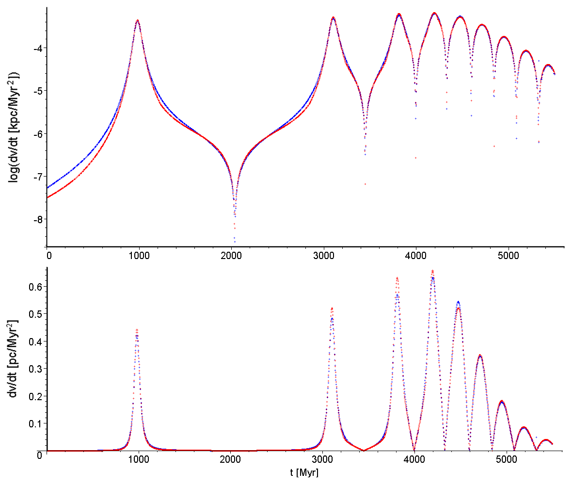
?figurename? 64: The logarithmic and linear plots of the time dependence of the dynamical friction for multiple passages of the secondary galaxy for the standard set of parameters (Sect. 17.5), using $b_{\mathrm{max}}=10$ kpc together with the lower limit of the Coulomb logarithm $\ln\Lambda_{\mathrm{crit}}=2$. Red values are computed in the model, blue values are numerical solution of Eq. (104).

Using a constant value of the Coulomb logarithm we did not obtain a good agreement between the friction calculated using the Chandrasekhar formula and using our method. The best option seems to be to calculate the value of the Coulomb logarithm in every step from the actual value of the velocity of the secondary galaxy. The $V_{0}$ in the definition Eq. (96) for $\Lambda$ is the difference between the velocities of the stars and the secondary galaxy. As the stellar velocities are isotropic, the average value is just the velocity of the secondary galaxy with respect to the center of the primary.

There is a uncertainty in the parameter $b_{\mathrm{max}}$ in the same equation – it should be theoretically equal to the distance between the center of the secondary and the outer boundary of the primary measured in the plane perpendicular to the motion of the secondary. But Eq. (100) assumes a homogeneous field of stars across all this distance, what is obviously not true. As the plane of the impact parameter is the plane perpendicular to the radial motion of the secondary galaxy, the density of the primary galaxy is always the highest in its center and decreases outwards. Thus it may seem that the $b_{\mathrm{max}}$ should be smaller than the normal distance to the edge of the primary galaxy, but the approximation of the $V_{0}$ with the velocity of the galaxy and other circumstances make the situation more complex. The value of $b_{\mathrm{max}}$ must be chosen in a trial-and-error method for the chosen parameters of collision so that the magnitude of the friction agrees best with the numerical solution of the integral Eq. (104).

The adaptive version of the Coulomb logarithm with a suitable chosen $b_{\mathrm{max}}$ fits nicely in the high velocity regime. The problem appears when the satellite gets close to its apocenter and also mainly in the late parts of the merger when the velocity of the satellite is much lower than during its first passage through the center of the primary galaxy. Here the adaptive version of the Coulomb logarithm with the chosen $b_{\mathrm{max}}$ significantly underestimates the friction when compared with the numerical solution of the integral Eq. (104). So we use the adaptive Coulomb logarithm until its value drops under a certain limit $\ln\Lambda_{\mathrm{crit}}$, then we put this limit for the Coulomb logarithm instead. With this modification of the Chandrasekhar formula, we can achieve a reasonable agreement, see Fig. 64. $b_{\mathrm{max}}$ and the lower limit for the Coulomb logarithm are free parameters and they depend on the parameters of the radial merger – the initial mutual velocity of the galaxies, their masses and Plummer radii.

E.3 Incorporation of the friction in the simulation

The question of incorporation of the dynamical friction in the simulations of the shell formation is tricky. In a fully self-consistent simulation, the dynamical friction would be automatically included, but such a simulation would be extremely demanding on resources – for the friction to be really well simulated, the number of particles of primary galaxy should not be several orders of magnitude smaller than the true amount of stars in the galaxies. Joining the stars in a smaller amount of more massive objects systematically overcounts the friction. Peñarrubia et al. (2004) remarked that Prugniel and Combes (1992); Wahde and Donner (1996) have indeed shown that the dynamical friction is artificially increased if the particle number is small. Using the analytical formula for the friction is not devoid of problems, but in some respects it could be more accurate than some of the self-consistent simulations.

On the other hand, the number of the particles of the secondary is an important quantity for the visibility of the shells in the simulations. And for the large number of required test particles $(\sim 10^{6})$ that represent just the secondary galaxy, even our “simple” simulations take hours of computation on a contemporary desktop computer. Furthermore, to explore the parameter space we have to run a lot of simulations, so we can really use a handy (semi-)analytical formula. We can easily add the acceleration calculated by Eq. (104) into the equation of motion of the galaxies.

It is worth mentioning that we departed in two aspects from the potential that we chose to model the merging galaxies. We assumed Maxwell velocity distribution, Eq. (99). This is not exactly true for the Plummer sphere, but the difference is small and the true velocity distribution in real galaxies is not known, so we cannot do much better, or say exactly how big mistake do we make.

The secondary galaxy is here treated as a point mass what artificially increases the friction, because the extended character of the galaxy softens the force (Sect. 17.2). Specially the stars with a small impact parameter with respect to the center of the secondary galaxy fly straight through it and their effect is significantly reduced compared to the Chandrasekhar formula for the point mass. The overestimation of the dynamical friction is not a crucial problem as we want to estimate how much the shell system is influenced by it – we can assume that the reality is not worse than our results and we get the upper bound on the effect.

?appendixname? F Tidal radius

For starters, let us remind the reader of the derivation of the tidal radius, as presented in Ebrová (2007). The tidal forces acting on an object are often derived using the following picture: A massive body (secondary galaxy) as a whole follows the force acting on it in its center of mass. But the force acting on outer parts of the body is different, as it is at different distances of the source (the primary galaxy). If this difference is larger than the binding force with the secondary for a given star, it is stripped off.

The tidal radius $r_{\mathrm{tidal}}$ is then defined as the distance (from the center of the secondary), where the difference of the force of the primary from its force in the center of mass of the secondary is just equal to the force from the secondary:

$$F_{\mathrm{p}}(d-r_{\mathrm{tidal}})-F_{\mathrm{p}}(d)=F_{\mathrm{s}}(r_{\mathrm{tidal}}),$$ (105)

where $d$ is the separation between the centers of the galaxies and $F_{\mathrm{p}}(r)$ and $F_{\mathrm{s}}(r)$ is the force from the primary and the secondary for a given test particle (its mass is immediately canceled out from the equation).

For two point-like bodies (with masses $M_{\mathrm{p}}$ and $M_{\mathrm{s}}$), we can write Eq. (105) as:

$$\frac{G\,M_{\mathrm{p}}}{d^{2}(1-r_{\mathrm{tidal}}/d)^{2}}-\frac{G\,M_{\mathrm{p}}}{d^{2}}=\frac{G\,M_{\mathrm{s}}}{r_{\mathrm{tidal}}^{2}}.$$ (106)

Assuming further $r_{\mathrm{tidal}}\ll d$ we can use the Taylor expansion $(1-x)^{-2}\cong 1+2x$ for $x=r_{\mathrm{tidal}}/d$ as it is then a small quantity. under this assumption we get a simple formula for the tidal radius:

$$r_{\mathrm{tidal}}=d\sqrt[3]{\frac{M_{\mathrm{s}}}{2\,M_{\mathrm{p}}}}.$$ (107)

However, for two point masses we can get an exact result for the tidal radius. Not making any approximation in Eq. (106) we can cast it as a fourth-order polynomial

$$X^{4}-2\,X^{3}+q\,X^{2}-2\,q\,X+q=0,$$ (108)

where $X=r_{\mathrm{tidal}}/d$ and $q=M_{\mathrm{s}}/M_{\mathrm{p}}$. A polynomial with an order less than five can be always solved. In our case, where $q$ is positive, there are two real roots, from which we take the one that gives $r_{\mathrm{tidal}}<d$ and thus $X<1$. The second real root corresponds to a point of the other side of the primary galaxy that is not of interest for us. The expression for this root does not give much insight, but an interested reader can find it in Appendix G.

?figurename? 65: Tidal radius for two point masses: the approximate solution, Eq. (107), is shown in blue, the exact solutions in red (the outer one in light red, the inner in dark red). The shows y-axis $X=r_{\mathrm{tidal}}/d$, the $x$-axis shows the secondary-to-primary mass ratio.

Eq. (105) gives the tidal radius for the particles on the line connecting the centers of the two bodies – we call it the inner tidal radius. Similarly we can write an equation for the particles on the other side of the secondary than the center of primary lies:

$$F_{\mathrm{p}}(d)-F_{\mathrm{p}}(d+r_{\mathrm{tidal}})=F_{\mathrm{s}}(r_{\mathrm{tidal}}).$$ (109)

It again leads to a fourth-order polynomial for which we can obtain the root that we call the outer tidal radius. The approximate solution Eq. (107) is the same for both equations, Eq. (105) and Eq. (109). Let us remark that the tidal radius is in any case just proportional to $d$ as there is no other scale in the problem. Fig. 65 shows the dependence of the three radii on the mass ratio of the bodies. We can see that for all relevant ratios the approximate formula is just between the inner and the outer tidal radius.

The tidal radius for a point mass is in some sense an oxymoron, as these objects have zero proportions by definition. For spherically symmetric bodies we can write Eq. (106) as

$$\frac{G\,M_{\mathrm{p}}(d-r_{\mathrm{tidal}})}{(d-r_{\mathrm{tidal}})^{2}}-\frac{G\,M_{\mathrm{p}}(d)}{d^{2}}=\frac{G\,M_{\mathrm{s}}(r_{\mathrm{tidal}})}{r_{\mathrm{tidal}}^{2}},$$ (110)

where $M(r)$ is the mass enclosed in the radius $r$. Particularly for the Plummer sphere we get this value integrating Eq. (74) over the sphere with the radius $r$:

$$M(r)=\frac{M}{(1+\varepsilon^{2}/r^{2})^{3/2}},$$ (111)

where $M$ is the overall mass of the body and $\varepsilon$ is the Plummer radius. Unfortunately this makes the equation too complex to be easily solved. Let us compare graphically the tidal radii for point masses and Plummer spheres of the same overall masses just for one particular case – Fig. 66.

The figure (or a simple thought) shows that the notion of the tidal radius in a general potential makes sense only when the force grows with the distance. Otherwise the tidal force acts in the same direction as the gravitation of the secondary and thus cannot strip off any mass. In the Plummer potential the force reaches its maximum in $\sqrt{2}\,\varepsilon/2$, so the tidal radius is not defined under this radius, whereas for the point masses it is defined everywhere.

The idea of the tidal radius is just an approximation to the complex processes during encounters of two extended bodies. It also does not define a sphere around the center of the secondary galaxy, but as we have seen, it is different for various locations, with the lowest value towards the center of the primary galaxy and the highest on the opposite side. For these reasons it is not really useful to improve its evaluation and so we have used the approximate Eq. (107) that as we have seen gives the values somewhere in the middle between the two extreme values of the tidal radius.

?figurename? 66: The outer and inner tidal radii (marked with circles) for the point masses and Plummer spheres with the secondary-to-primary mass ratio of 0.02. In the Plummer case, the Plummer radius of the primary is 0.5 of the distance between the bodies and the Plummer radius of the secondary is 0.1 of the same quantity. Blue lines (light blue for the point mass, dark blue for the Plummer sphere) show the gravitational force of the primary in arbitrary units, red lines (light red for the point mass, dark red for the Plummer sphere) show the difference between the gravitational force of the primary in a given point and its value in 1, where the center of the secondary is. The tidal radii are the points of intersection of corresponding curves.

?appendixname? G Expressions for the tidal radius

Here we give the analytical formulae for the tidal radii in the system of two point masses as discussed in Appendix F. For the inner tidal radius we have:

$$\frac{r}{d}=\frac{1}{2}+\frac{\sqrt{3}}{6}\left(\frac{\sqrt{y}}{\sqrt[6]{z}}-\sqrt{6-4\,q-\sqrt[3]{qz}-\sqrt[3]{\frac{q^{5}}{z}}+6\,\sqrt[6]{z}\sqrt{\frac{3}{y}}(q+1)}\,\right),$$ (112)

where

$$y=(3-2\,q)\sqrt[3]{z}+\sqrt[3]{qz^{2}}+q^{5/3}$$ (113)

$$z=54+q^{2}+6\,\sqrt{81+3\,q^{2}}$$ (114)

and for the outer tidal radius we get similar expressions:

$$\frac{r}{d}=\frac{1}{2}+\frac{\sqrt{3}}{6}\left(\frac{\sqrt{u}}{\sqrt[6]{v}}+\sqrt{6+4\,q-\sqrt[3]{qv}-\sqrt[3]{\frac{q^{5}}{v}}+6\,\sqrt[6]{v}\sqrt{\frac{3}{u}}(q-1)}\,\right),$$ (115)

where

$$u=(3+2\,q)\sqrt[3]{v}+\sqrt[3]{qv^{2}}+q^{5/3}$$ (116)

$$v=-54-q^{2}+6\,\sqrt{81+3\,q^{2}}$$ (117)

and in all the expressions we use

$$q=\frac{M_{\mathrm{s}}}{M_{\mathrm{p}}}.$$ (118)

?appendixname? H Videos

Several videos are also part of the electronic attachment of the thesis. Here we present their description. Information on details of the simulation process can be found in Sect. 17. The videos can be also downloaded at: pc048b.fzu.cz/$\sim$ivana/shells/phd

1. 1-shells.avi – Video from a simulation of a shell-producing radial minor merger from a perspective perpendicular to the axis of the merger. The bottom three panels show an area of $60\times 60$ kpc centered on the primary which is the zoomed part of the upper panels of size $300\times 300$ kpc. The first column shows the surface density of both the primary and the secondary galaxy, the second only the surface density of the particles originally belonging to the secondary galaxy (corresponding to the host galaxy subtraction, a technique used in processing real galaxy images). The third column shows the surface density of particles originally belonging to the secondary galaxy divided by the surface density of the primary galaxy (also corresponding to an observational technique). The parameters of the merger are the following: the mass of the primary is $3\times 10^{11}$ M_⊙ , the secondary-to-primary mass ratio is 0.02, the Plummer radius of the primary is 7.6 kpc, of the secondary 0.76 kpc. The initial relative velocity of the galaxies was equal to the escape velocity of the secondary and the separation of their centers was 90 kpc. When the centers of the galaxies pass through each other, the potential of the secondary is suddenly switched off.

2. 2-shells.mpg – Video from a simulation of a shell-producing radial minor merger used in Sect. 13. The top panel ($300\times 300$ kpc centered on primary) shows the surface density of the particles originally belonging to the secondary galaxy from a perspective perpendicular to the axis of the merger; the bottom panel shows the density of the particles originally belonging to the secondary in the space of radial velocity (vertical axis) versus galactocentric distance (horizontal axis). The potential of the host galaxy is the same as the one described in Sect. 8.1. Primary is modeled as a double Plummer sphere with respective masses $M_{*}=2\times 10^{11}$ M_⊙ and $M_{\mathrm{DM}}=1.2\times 10^{13}$ M_⊙ , and Plummer radii $\varepsilon_{*}=5$ kpc and $\varepsilon_{\mathrm{DM}}=100$ kpc for the luminous component and the dark halo, respectively. The potential of the cannibalized galaxy is chosen to be a single Plummer sphere with the total mass $M=2\times 10^{10}$ M_⊙ and Plummer radius $\varepsilon_{*}=2$ kpc. The cannibalized galaxy is released from rest at a distance of 100 kpc from the center of the host galaxy. When it reaches the center of the host galaxy in 306.4 Myr, its potential is switched off and its particles begin to oscillate freely in the host galaxy.

3. 3-projection.mpg – Video shoes the simulation from point 2 (used in Sect. 13) at the time 2.2 Gyr after the decay of the cannibalized galaxy (2.5 Gyr of the simulation time) from different perspectives. Angle of 0 degrees corresponds to the perspective perpendicular to the axis of the merger.

4. 4-friction.avi – Surface density of the particles originally belonging to the secondary galaxy from two simulation of a radial minor merger from Sect. 22.1 (run 1 – right panels and run 2 – left panels). The first column corresponds to the simulation with dynamical friction and gradual decay of the secondary; the other corresponds to the simulation without friction and with the instant disruption of the secondary near the center of the primary galaxy. The bottom panels show an area of $60\times 60$ kpc centered on the primary which is the zoomed part of the upper panels of size $300\times 300$ kpc. The video covers 8 Gyr since the release of the secondary galaxy from distance of 180 kpc from the center of the primary with the escape velocity. Both simulations were executed for the the standard set of parameters (Sect. 17.5): the mass of the primary is $3.2\times 10^{11}$ M_⊙ , the secondary-to-primary mass ratio is 0.02, the Plummer radius of the primary is 20 kpc, of the secondary 2 kpc.

5. 5-selfconsistent.avi – Video from self-consistent simulation of a radial minor merger from Sect. 22.3. The bottom panel ($400\times 400$ kpc centered on primary) shows the surface density of the particles originally belonging to the secondary galaxy from a perspective perpendicular to the axis of the merger; the top panel shows the density of the particles originally belonging to the secondary in the space of radial velocity (vertical axis) versus galactocentric distance (horizontal axis). The potential of the primary galaxy is a double Plummer sphere with respective masses $M_{*}=2\times 10^{11}$ M_⊙ and $M_{\mathrm{DM}}=8\times 10^{12}$ M_⊙ , and Plummer radii $\varepsilon_{*}=8$ kpc and $\varepsilon_{\mathrm{DM}}=20$ kpc for the luminous component and the dark halo, respectively. The potential of the secondary galaxy is chosen to be a single Plummer sphere with the total mass $M=2\times 10^{10}$ M_⊙ and Plummer radius $\varepsilon_{*}=2$ kpc. The cannibalized galaxy is released from the distance of 200 kpc from the center of the host galaxy with the initial velocity 102 km$/$s.

Videos 2–4 were made from simulated data by Miroslav Křížek.