PyFR: An Open Source Framework for Solving Advection-Diffusion Type Problems on Streaming Architectures using the Flux Reconstruction Approach

Abstract

High-order numerical methods for unstructured grids combine the superior accuracy of high-order spectral or finite difference methods with the geometric flexibility of low-order finite volume or finite element schemes. The Flux Reconstruction (FR) approach unifies various high-order schemes for unstructured grids within a single framework. Additionally, the FR approach exhibits a significant degree of element locality, and is thus able to run efficiently on modern streaming architectures, such as Graphical Processing Units (GPUs). The aforementioned properties of FR mean it offers a promising route to performing affordable, and hence industrially relevant, scale-resolving simulations of hitherto intractable unsteady flows within the vicinity of real-world engineering geometries. In this paper we present PyFR, an open-source Python based framework for solving advection-diffusion type problems on streaming architectures using the FR approach. The framework is designed to solve a range of governing systems on mixed unstructured grids containing various element types. It is also designed to target a range of hardware platforms via use of an in-built domain specific language based on the Mako templating engine. The current release of PyFR is able to solve the compressible Euler and Navier-Stokes equations on grids of quadrilateral and triangular elements in two dimensions, and hexahedral elements in three dimensions, targeting clusters of CPUs, and NVIDIA GPUs. Results are presented for various benchmark flow problems, single-node performance is discussed, and scalability of the code is demonstrated on up to 104 NVIDIA M2090 GPUs. The software is freely available under a 3-Clause New Style BSD license (see www.pyfr.org).

Keywords: High-order; Flux reconstruction; Parallel algorithms; Heterogeneous computing

Program Description

Authors

F. D. Witherden, A. M. Farrington, P. E. Vincent

Program title

PyFR v0.1.0

Licensing provisions

New Style BSD license

Programming language

Python, CUDA and C

Computer

Variable, up to and including GPU clusters

Operating system

Recent version of Linux/UNIX

RAM

Variable, from hundreds of megabytes to gigabytes

Number of processors used

Variable, code is multi-GPU and multi-CPU aware through a combination of MPI and OpenMP

External routines/libraries

Python 2.7, numpy, PyCUDA, mpi4py, SymPy, Mako

Nature of problem

Compressible Euler and Navier-Stokes equations of fluid dynamics; potential for any advection-diffusion type problem.

Solution method

High-order flux reconstruction approach suitable for curved, mixed, unstructured grids.

Unusual features

Code makes extensive use of symbolic manipulation and run-time code generation through a domain specific language.

Running time

Many small problems can be solved on a recent workstation in minutes to hours.

Nomenclature

Throughout we adopt a convention in which dummy indices on the right hand side of an expression are summed. For example $C_{ijk}=A_{ijl}B_{ilk}\equiv\sum_{l}A_{ijl}B_{ilk}$ where the limits are implied from the surrounding context. All indices are assumed to be zero-based.

Functions.
$\delta_{ij}$	Kronecker delta
$\det\bm{\mathsf{A}}$	Matrix determinant
$\dim\bm{\mathsf{A}}$	Matrix dimensions
Indices.
$e$	Element type
$n$	Element number
$\alpha$	Field variable number
$i,j,k$	Summation indices
$\rho,\sigma,\nu$	Summation indices
Domains.
$\mathbf{\Omega}$	Solution domain
$\mathbf{\Omega}_{e}$	All elements in $\mathbf{\Omega}$ of type $e$
$\hat{\mathbf{\Omega}}_{e}$	A standard element of type $e$
$\partial\hat{\mathbf{\Omega}}_{e}$	Boundary of $\hat{\mathbf{\Omega}}_{e}$
$\mathbf{\Omega}_{en}$	Element $n$ of type $e$ in $\mathbf{\Omega}$
$\left\lvert\mathbf{\Omega}_{e}\right\rvert$	Number of elements of type $e$
Expansions.
$\wp$	Polynomial order
$N_{D}$	Number of spatial dimensions
$N_{V}$	Number of field variables
$\ell_{e\rho}$	Nodal basis polynomial $\rho$ for element type $e$
$x,y,z$	Physical coordinates
$\tilde{x},\tilde{y},\tilde{z}$	Transformed coordinates
$\bm{\mathcal{M}}_{en}$	Transformed to physical mapping
Adornments and suffixes.
$\tilde{\square}$	A quantity in transformed space
$\hat{\square}$	A vector quantity of unit magnitude
$\square^{T}$	Transpose
$\square^{(u)}$	A quantity at a solution point
$\square^{(f)}$	A quantity at a flux point
$\square^{(f_{\perp})}$	A normal quantity at a flux point
Operators.
$\mathfrak{C}_{\alpha}$	Common solution at an interface
$\mathfrak{F}_{\alpha}$	Common normal flux at an interface

1 Introduction

There is an increasing desire amongst industrial practitioners of computational fluid dynamics (CFD) to undertake high-fidelity scale-resolving simulations of transient compressible flows within the vicinity of complex geometries. For example, to improve the design of next generation unmanned aerial vehicles (UAVs), there exists a need to perform simulations—at Reynolds numbers $10^{4}$–$10^{7}$ and Mach numbers $M\sim 0.1$–$1.0$—of highly separated flow over deployed spoilers/air-brakes; separated flow within serpentine intake ducts; acoustic loading in weapons bays; and flow over entire UAV configurations at off-design conditions. Unfortunately, current generation industry-standard CFD software based on first- or second-order accurate Reynolds Averaged Navier-Stokes (RANS) approaches is not well suited to performing such simulations. Henceforth, there has been significant interest in the potential of high-order accurate methods for unstructured mixed grids, and whether they can offer an efficient route to performing scale-resolving simulations within the vicinity of complex geometries. Popular examples of high-order schemes for unstructured mixed grids include the discontinuous Galerkin (DG) method, first introduced by Reed and Hill [1], and the spectral difference (SD) methods originally proposed under the moniker ‘staggered-gird Chebyshev multidomain methods’ by Kopriva and Kolias in 1996 [2] and later popularised by Sun et al. [3]. In 2007 Huynh proposed the flux reconstruction (FR) approach [4]; a unifying framework for high-order schemes for unstructured grids that incorporates both the nodal DG schemes of [5] and, at least for a linear flux function, any SD scheme. In addition to offering high-order accuracy on unstructured mixed grids, FR schemes are also compact in space, and thus when combined with explicit time marching offer a significant degree of element locality. As such, explicit high-order FR schemes are characterised by a large degree of structured computation.

Over the past two decades improvements in the arithmetic capabilities of processors have significantly outpaced advances in random access memory. Algorithms which have traditionally been compute bound—such as dense matrix-vector products—are now limited instead by the bandwidth to/from memory. This is epitomised in Figure 1. Whereas the processors of two decades ago had FLOPS-per-byte of ${\sim}0.2$ more recent chips have ratios upwards of ${\sim}4$. This disparity is not limited to just conventional CPUs. Massively parallel accelerators and co-processors such as the NVIDIA K20X and Intel Xeon Phi 5110P have ratios of $5.24$ and $3.16$, respectively.

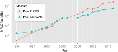
Figure 1: Trends in the peak floating point performance (double precision) and memory bandwidth of sever-class Intel processors from 1994–2013. The quotient of these two measures yields the FLOPS-per-byte of a processor. Data courtesy of Jan Treibig.

A concomitant of this disparity is that modern hardware architectures are highly dependent on a combination of high speed caches and/or shared memory to maintain throughput. However, for an algorithm to utilise these efficiently its memory access pattern must exhibit a degree of either spatial or temporal locality. To a first-order approximation the spatial locality of a method is inversely proportional to the amount of memory indirection. On an unstructured grid indirection arises whenever there is coupling between elements. This is potentially a problem for discretisations whose stencil is not compact. Coupling also arises in the context of implicit time stepping schemes. Implementations are therefore very often bound by memory bandwidth. As a secondary trend we note that the manner in which FLOPS are realised has also changed. In the early 1990s commodity CPUs were predominantly scalar with a single core of execution. However in 2013 processors with eight or more cores are not uncommon. Moreover, the cores on modern processors almost always contain vector processing units. Vector lengths up to 256-bits, which permit up to four double precision values to be operated on at once, are not uncommon. It is therefore imperative that compute-bound algorithms are amenable to both multithreading and vectorisation. A versatile means of accomplishing this is by breaking the computation down into multiple, necessarily independent, streams. By virtue of their independence these streams can be readily divided up between cores and vector lanes. This leads directly to the concept of stream processing. We will refer to architectures amenable to this form of parallelisation as streaming architectures.

A corollary of the above discussion is that compute intensive discretisations which can be formulated within the stream processing paradigm are well suited to acceleration on current—and likely future—hardware platforms. The FR approach combined with explicit time stepping is an archetypical of this.

Our objective in this paper is to present PyFR, an open-source Python based framework for solving advection-diffusion type problems on streaming architectures using the FR approach. The framework is designed to solve a range of governing systems on mixed unstructured grids containing various element types. It is also designed to target a range of hardware platforms via use of an in-built domain specific language derived from the Mako templating engine. The current release of PyFR is able to solve the compressible Euler and Navier-Stokes equations on unstructured grids of quadrilateral and triangular elements in two-dimensions, and unstructured grids of hexahedral elements in three-dimensions, targeting clusters of CPUs, and NVIDIA GPUs. The paper is structured as follows. In section 2 we provide a overview of the FR approach for advection-diffusion type problems on mixed unstructured grids. In section 3 we proceed to describe our implementation strategy, and in section 4 we present the Euler and Navier-Stokes equations, which are solved by the current release of PyFR. The framework is then validated in section 5, single-node performance is discussed in section 6, and scalability of the code is demonstrated on up to 104 NVIDIA M2090 GPUs in section 7. Finally, conclusions are drawn in section 8.

2 Flux Reconstruction

A brief overview of the FR approach for solving advection-diffusion type problems is given below. Extended presentations can be found elsewhere [4, 6, 7, 8, 9, 10, 11, 12, 13, 14].

Consider the following advection-diffusion problem inside an arbitrary domain $\mathbf{\Omega}$ in $N_{D}$ dimensions

$$\frac{\partial u_{\alpha}}{\partial t}+\bm{\nabla}\cdot\mathbf{f}_{\alpha}=0,$$ (1)

where $0\leq\alpha<N_{V}$ is the field variable index, $u_{\alpha}=u_{\alpha}(\mathbf{x},t)$ is a conserved quantity, $\mathbf{f}_{\alpha}=\mathbf{f}_{\alpha}(u,\bm{\nabla}u)$ is the flux of this conserved quantity and $\mathbf{x}=x_{i}\in\mathbb{R}^{N_{D}}$. In defining the flux we have taken $u$ in its unscripted form to refer to all of the $N_{V}$ field variables and $\bm{\nabla}u$ to be an object of length $N_{D}\times N_{V}$ consisting of the gradient of each field variable. We start by rewriting Equation 1 as a first order system

$$\frac{\partial u_{\alpha}}{\partial t}+\bm{\nabla}\cdot\mathbf{f}_{\alpha}(u,\mathbf{q}) =0,$$ (2a)

$$\mathbf{q}_{\alpha}-\bm{\nabla}u_{\alpha} =0,$$ (2b)

where $\mathbf{q}$ is an auxiliary variable. Here, as with $\bm{\nabla}u$, we have taken $\mathbf{q}$ in its unsubscripted form to refer to the gradients of all of the field variables.

Take $\mathcal{E}$ to be the set of available element types in $\mathbb{R}^{N_{D}}$. Examples include quadrilaterals and triangles in two dimensions and hexahedra, prisms, pyramids and tetrahedra in three dimensions. Consider using these various elements types to construct a conformal mesh of the domain such that

$$\mathbf{\Omega}=\bigcup_{e\in\mathcal{E}}\mathbf{\Omega}_{e}\qquad\text{and}\qquad\mathbf{\Omega}_{e}=\bigcup_{n=0}^{|\mathbf{\Omega}_{e}|-1}\mathbf{\Omega}_{en}\qquad\text{and}\qquad\bigcap_{e\in\mathcal{E}}\bigcap_{n=0}^{|\mathbf{\Omega}_{e}|-1}\mathbf{\Omega}_{en}=\emptyset,$$

where $\mathbf{\Omega}_{e}$ refers to all of the elements of type $e$ inside of the domain, $\left\lvert\mathbf{\Omega}_{e}\right\rvert$ is the number of elements of this type in the decomposition, and $n$ is an index running over these elements with $0\leq n<\left\lvert\mathbf{\Omega}_{e}\right\rvert$. Inside each element $\mathbf{\Omega}_{en}$ we require that

$$\frac{\partial u_{en\alpha}}{\partial t}+\bm{\nabla}\cdot\mathbf{f}_{en\alpha} =0,$$ (3a)

$$\mathbf{q}_{en\alpha}-\bm{\nabla}u_{en\alpha} =0.$$ (3b)

It is convenient, for reasons of both mathematical simplicity and computational efficiency, to work in a transformed space. We accomplish this by introducing, for each element type, a standard element $\mathbf{\hat{\Omega}}_{e}$ which exists in a transformed space, $\tilde{\mathbf{x}}=\tilde{x}_{i}$. Next, assume the existence of a mapping function for each element such that

$$x_{i} =\mathcal{M}_{eni}(\tilde{\mathbf{x}}), \mathbf{x} =\bm{\mathcal{M}}_{en}(\tilde{\mathbf{x}}),$$

$$\tilde{x}_{i} =\mathcal{M}^{-1}_{eni}(\mathbf{x}), \tilde{\mathbf{x}} =\bm{\mathcal{M}}^{-1}_{en}(\mathbf{x}),$$

along with the relevant Jacobian matrices

$$\bm{\mathsf{J}}_{en}=J_{enij} =\frac{\partial\mathcal{M}_{eni}}{\partial\tilde{x}_{j}}, J_{en} =\det\bm{\mathsf{J}}_{en},$$

$$\bm{\mathsf{J}}^{-1}_{en}=J^{-1}_{enij} =\frac{\partial\mathcal{M}^{-1}_{eni}}{\partial x_{j}}, J^{-1}_{en} =\det\bm{\mathsf{J}}^{-1}_{en}=\frac{1}{J_{en}}.$$

These definitions provide us with a means of transforming quantities to and from standard element space. Taking the transformed solution, flux, and gradients inside each element to be

$$\tilde{u}_{en\alpha} =\tilde{u}_{en\alpha}(\tilde{\mathbf{x}},t)=J_{en}(\tilde{\mathbf{x}})u_{en\alpha}(\bm{\mathcal{M}}_{en}(\tilde{\mathbf{x}}),t),$$ (4a)

$$\tilde{\mathbf{f}}_{en\alpha} =\tilde{\mathbf{f}}_{en\alpha}(\tilde{\mathbf{x}},t)=J_{en}(\tilde{\mathbf{x}})\bm{\mathsf{J}}^{-1}_{en}(\bm{\mathcal{M}}_{en}(\tilde{\mathbf{x}}))\mathbf{f}_{en\alpha}(\bm{\mathcal{M}}_{en}(\tilde{\mathbf{x}}),t),$$ (4b)

$$\tilde{\mathbf{q}}_{en\alpha} =\tilde{\mathbf{q}}_{en\alpha}(\tilde{\mathbf{x}},t)=\bm{\mathsf{J}}^{T}_{en}(\tilde{\mathbf{x}})\mathbf{q}_{en\alpha}(\bm{\mathcal{M}}_{en}(\tilde{\mathbf{x}}),t),$$ (4c)

and letting $\tilde{\bm{\nabla}}=\partial/\partial\tilde{x}_{i}$, it can be readily verified that

$$\frac{\partial u_{en\alpha}}{\partial t}+J^{-1}_{en}\tilde{\bm{\nabla}}\cdot\tilde{\mathbf{f}}_{en\alpha} =0,$$ (5a)

$$\tilde{\mathbf{q}}_{en\alpha}-\tilde{\bm{\nabla}}u_{en\alpha} =0,$$ (5b)

as required. We note here the decision to multiply the first equation through by a factor of $J^{-1}_{en}$. Doing so has the effect of taking $\tilde{u}_{en}\mapsto u_{en}$ which allows us to work in terms of the physical solution. This is more convenient from a computational standpoint.

We next proceed to associate a set of solution points with each standard element. For each type $e\in\mathcal{E}$ take $\set{\tilde{\mathbf{x}}^{(u)}_{e\rho}}$ to be the chosen set of points where $0\leq\rho<N^{(u)}_{e}(\wp)$. These points can then be used to construct a nodal basis set $\set{\ell^{(u)}_{e\rho}(\tilde{\mathbf{x}})}$ with the property that $\ell^{(u)}_{e\rho}(\tilde{\mathbf{x}}^{(u)}_{e\sigma})=\delta_{\rho\sigma}$. To obtain such a set we first take $\set{\psi_{e\sigma}(\tilde{\mathbf{x}})}$ to be any basis which spans a selected order $\wp$ polynomial space defined inside $\hat{\mathbf{\Omega}}_{e}$. Next we compute the elements of the generalised Vandermonde matrix $\mathcal{V}_{e\rho\sigma}=\psi_{e\rho}(\tilde{\mathbf{x}}^{(u)}_{e\sigma})$. With these a nodal basis set can be constructed as $\ell^{(u)}_{e\rho}(\tilde{\mathbf{x}})=\mathcal{V}^{-1}_{e\rho\sigma}\psi_{e\sigma}(\tilde{\mathbf{x}})$. Along with the solution points inside of each element we also define a set of flux points on $\partial\hat{\mathbf{\Omega}}_{e}$. We denote the flux points for a particular element type as $\set{\tilde{\mathbf{x}}^{(f)}_{e\rho}}$ where $0\leq\rho<N^{(f)}_{e}(\wp)$. Let the set of corresponding normalised outward-pointing normal vectors be given by $\set{\hat{\tilde{\mathbf{n}}}^{(f)}_{e\rho}}$. It is critical that each flux point pair along an interface share the same coordinates in physical space. For a pair of flux points $e\rho n$ and $e^{\prime}\rho^{\prime}n^{\prime}$ at a non-periodic interface this can be formalised as $\bm{\mathcal{M}}_{en}(\tilde{\mathbf{x}}^{(f)}_{e\rho})=\bm{\mathcal{M}}_{e^{\prime}n^{\prime}}(\tilde{\mathbf{x}}^{(f)}_{e^{\prime}\rho^{\prime}})$. A pictorial illustration of this can be seen in Figure 2.

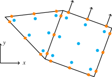
Figure 2: Solution points (blue circles) and flux points (orange squares) for a triangle and quadrangle in physical space. For the top edge of the quadrangle the normal vectors have been plotted. Observe how the flux points at the interface between the two elements are co-located.

The first step in the FR approach is to go from the discontinuous solution at the solution points to the discontinuous solution at the flux points

$$u^{(f)}_{e\sigma n\alpha}=u^{(u)}_{e\rho n\alpha}\ell^{(u)}_{e\rho}(\tilde{\mathbf{x}}^{(f)}_{e\sigma}),$$ (6)

where $u^{(u)}_{e\rho n\alpha}$ is an approximate solution of field variable $\alpha$ inside of the $n$th element of type $e$ at solution point $\tilde{\mathbf{x}}^{(u)}_{e\rho}$. This can then be used to compute a common solution

$$\mathfrak{C}^{\vphantom{(f)}}_{\vphantom{\widetilde{e\rho n}\alpha}\alpha}u^{(f)}_{\vphantom{\widetilde{e\rho n}\alpha}e\rho n\alpha}=\mathfrak{C}^{\vphantom{(f)}}_{\vphantom{\widetilde{e\rho n}\alpha}\alpha}u^{(f)}_{\widetilde{e\rho n}\alpha}=\mathfrak{C}^{\vphantom{(f)}}_{\vphantom{\widetilde{e\rho n}\alpha}\alpha}(u^{(f)}_{\vphantom{\widetilde{e\rho n}\alpha}e\rho n\alpha},u^{(f)}_{\widetilde{e\rho n}\alpha}),$$ (7)

where $\mathfrak{C}_{\alpha}(u_{L},u_{R})$ is a scalar function that given two values at a point returns a common value. Here we have taken $\widetilde{e\rho n}$ to be the element type, flux point number and element number of the adjoining point at the interface. Since grids in FR are permitted to be unstructured the relationship between $e\rho n$ and $\widetilde{e\rho n}$ is indirect. This necessitates the use of a lookup table. As the common solution function is permitted to perform upwinding or downwinding of the solution it is in general the case that $\mathfrak{C}^{\vphantom{(f)}}_{\vphantom{\widetilde{e\rho n}\alpha}\alpha}(u^{(f)}_{\vphantom{\widetilde{e\rho n}\alpha}e\rho n\alpha},u^{(f)}_{\widetilde{e\rho n}\alpha})\neq\mathfrak{C}^{\vphantom{(f)}}_{\vphantom{\widetilde{e\rho n}\alpha}\alpha}(u^{(f)}_{\widetilde{e\rho n}\alpha},u^{(f)}_{\vphantom{\widetilde{e\rho n}\alpha}e\rho n\alpha})$. Hence, it is important that each flux point pair only be visited once with the same common solution value assigned to both $\mathfrak{C}^{\vphantom{(f)}}_{\vphantom{\widetilde{e\rho n}\alpha}\alpha}u^{(f)}_{\vphantom{\widetilde{e\rho n}\alpha}e\rho n\alpha}$ and $\mathfrak{C}^{\vphantom{(f)}}_{\vphantom{\widetilde{e\rho n}\alpha}\alpha}u^{(f)}_{\widetilde{e\rho n}\alpha}$.

Further, associated with each flux point is a vector correction function $\mathbf{g}^{(f)}_{e\rho}(\tilde{\mathbf{x}})$ constrained such that

$$\hat{\tilde{\mathbf{n}}}^{(f)}_{e\sigma}\cdot\mathbf{g}^{(f)}_{e\rho}(\tilde{\mathbf{x}}^{(f)}_{e\sigma})=\delta_{\rho\sigma},$$ (8)

with a divergence that sits in the same polynomial space as the solution. Using these fields we can express the solution to Equation 5b as

$$\tilde{\mathbf{q}}^{(u)}_{e\sigma n\alpha}=\bigg{[}\hat{\tilde{\mathbf{n}}}^{(f)}_{e\rho}\cdot\tilde{\bm{\nabla}}\cdot\mathbf{g}^{(f)}_{e\rho}(\tilde{\mathbf{x}})\left\{\mathfrak{C}^{\vphantom{(f)}}_{\alpha}u^{(f)}_{e\rho n\alpha}-u^{(f)}_{e\rho n\alpha}\right\}+u^{(u)}_{e\nu n\alpha}\tilde{\bm{\nabla}}\ell^{(u)}_{e\nu}(\tilde{\mathbf{x}})\bigg{]}_{\tilde{\mathbf{x}}=\tilde{\mathbf{x}}^{(u)}_{e\sigma}},$$ (9)

where the term inside the curly brackets is the ‘jump’ at the interface and the final term is an order $\wp-1$ approximation of the gradient obtained by differentiating the discontinuous solution polynomial. Following the approaches of Kopriva [15] and Sun et al. [3] we can now compute physical gradients as

$$\mathbf{q}^{(u)}_{e\sigma n\alpha} =\bm{\mathsf{J}}^{-T\,(u)}_{e\sigma n}\tilde{\mathbf{q}}^{(u)}_{e\sigma n\alpha},$$ (10)

$$\mathbf{q}^{(f)}_{e\sigma n\alpha} =\ell^{(u)}_{e\rho}(\tilde{\mathbf{x}}^{(f)}_{e\sigma})\mathbf{q}^{(u)}_{e\rho n\alpha},$$ (11)

where $\bm{\mathsf{J}}^{-T\,(u)}_{e\sigma n}=\bm{\mathsf{J}}^{-T}_{en}(\tilde{\mathbf{x}}^{(u)}_{e\sigma})$. Having solved the auxiliary equation we are now able to evaluate the transformed flux

$$\tilde{\mathbf{f}}^{(u)}_{e\rho n\alpha}=J^{(u)}_{e\rho n}\bm{\mathsf{J}}^{-1\,(u)}_{e\rho n}\mathbf{f}_{\alpha}(u^{(u)}_{e\rho n},\mathbf{q}^{(u)}_{e\rho n}),$$ (12)

where $J^{(u)}_{e\rho n}=\det\bm{\mathsf{J}}_{en}(\tilde{\mathbf{x}}^{(u)}_{e\rho})$. This can be seen to be a collocation projection of the flux. With this it is possible to compute the normal transformed flux at each of the flux points

$$\tilde{f}^{(f_{\perp})}_{e\sigma n\alpha}=\ell^{(u)}_{e\rho}(\tilde{\mathbf{x}}^{(f)}_{e\sigma})\hat{\tilde{\mathbf{n}}}^{(f)}_{e\sigma}\cdot\tilde{\mathbf{f}}^{(u)}_{e\rho n\alpha}.$$ (13)

Considering the physical normals at the flux points we see that

$$\mathbf{n}^{(f)}_{e\sigma n}=n^{(f)}_{e\sigma n}\hat{\mathbf{n}}^{(f)}_{e\sigma n}=\bm{\mathsf{J}}^{-T\,(f)}_{e\sigma n}\hat{\tilde{\mathbf{n}}}^{(f)}_{e\sigma},$$ (14)

which is the outward facing normal vector in physical space where $n^{(f)}_{e\sigma n}>0$ is defined as the magnitude. As the interfaces between two elements conform we must have $\hat{\mathbf{n}}^{(f)}_{\vphantom{\widetilde{e\sigma n}}e\sigma n}=-\hat{\mathbf{n}}^{(f)}_{\widetilde{e\sigma n}}$. With these definitions we are now in a position to specify an expression for the common normal flux at a flux point pair as

$$\mathfrak{F}^{\vphantom{(f)}}_{\vphantom{\widetilde{e\sigma n}}\alpha}f^{(f_{\perp})}_{\vphantom{\widetilde{e\sigma n}}e\sigma n\alpha}=-\mathfrak{F}^{\vphantom{(f)}}_{\vphantom{\widetilde{e\sigma n}}\alpha}f^{(f_{\perp})}_{\widetilde{e\sigma n}\alpha}=\mathfrak{F}^{\vphantom{(f)}}_{\vphantom{\widetilde{e\sigma n}}\alpha}(u^{(f)}_{\vphantom{\widetilde{e\sigma n}}e\sigma n},u^{(f)}_{\widetilde{e\sigma n}},\mathbf{q}^{(f)}_{\vphantom{\widetilde{e\sigma n}}e\sigma n},\mathbf{q}^{(f)}_{\widetilde{e\sigma n}},\hat{\mathbf{n}}^{(f)}_{\vphantom{\widetilde{e\sigma n}}e\sigma n}).$$ (15)

The relationship $\mathfrak{F}^{\vphantom{(f)}}_{\vphantom{\widetilde{e\sigma n}}\alpha}f^{(f_{\perp})}_{\vphantom{\widetilde{e\sigma n}}e\sigma n\alpha}=-\mathfrak{F}^{\vphantom{(f)}}_{\vphantom{\widetilde{e\sigma n}}\alpha}f^{(f_{\perp})}_{\widetilde{e\sigma n}\alpha}$ arises from the desire for the resulting numerical scheme to be conservative; a net outward flux from one element must be balanced by a corresponding inward flux on the adjoining element. It follows that that $\mathfrak{F}_{\alpha}(u_{L},u_{R},\mathbf{q}_{L},\mathbf{q}_{R},\hat{\mathbf{n}}_{L})=-\mathfrak{F}_{\alpha}(u_{R},u_{L},\mathbf{q}_{R},\mathbf{q}_{L},-\hat{\mathbf{n}}_{L})$. The common normal fluxes in Equation 15 can now be taken into transformed space via

$$\mathfrak{F}^{\vphantom{(f_{\perp})}}_{\alpha}\tilde{f}^{(f_{\perp})}_{e\sigma n\alpha} =J^{(f)}_{e\sigma n}n^{(f)}_{e\sigma n}\mathfrak{F}_{\alpha}f^{(f_{\perp})}_{e\sigma n\alpha},$$ (16)

$$\mathfrak{F}^{\vphantom{(f_{\perp})}}_{\vphantom{\widetilde{e\sigma n}}\alpha}\tilde{f}^{(f_{\perp})}_{\widetilde{e\sigma n}\alpha} =J^{(f)}_{\widetilde{e\sigma n}}n^{(f)}_{\widetilde{e\sigma n}}\mathfrak{F}^{\vphantom{(f_{\perp})}}_{\vphantom{\widetilde{e\sigma n}}\alpha}f^{(f_{\perp})}_{\widetilde{e\sigma n}\alpha},$$ (17)

where $J^{(f)}_{e\sigma n}=\det\bm{\mathsf{J}}_{en}(\tilde{\mathbf{x}}^{(f)}_{e\sigma})$.

It is now possible to compute an approximation for the divergence of the continuous flux. The procedure is directly analogous to the one used to calculate the transformed gradient in Equation 9

$$(\tilde{\bm{\nabla}}\cdot\tilde{\mathbf{f}})^{(u)}_{e\rho n\alpha}=\bigg{[}\tilde{\bm{\nabla}}\cdot\mathbf{g}^{(f)}_{e\sigma}(\tilde{\mathbf{x}})\left\{\mathfrak{F}^{\vphantom{(f)}}_{\alpha}\tilde{f}^{(f_{\perp})}_{e\sigma n\alpha}-\tilde{f}^{(f_{\perp})}_{e\sigma n\alpha}\right\}+\tilde{\mathbf{f}}^{(u)}_{e\nu n\alpha}\cdot\tilde{\bm{\nabla}}\ell^{(u)}_{e\nu}(\tilde{\mathbf{x}})\bigg{]}_{\tilde{\mathbf{x}}=\tilde{\mathbf{x}}^{(u)}_{e\rho}},$$ (18)

which can then be used to obtain a semi-discretised form of the governing system

$$\frac{\partial u^{(u)}_{e\rho n\alpha}}{\partial t}=-J^{-1\,(u)}_{e\rho n}(\tilde{\bm{\nabla}}\cdot\tilde{\mathbf{f}})^{(u)}_{e\rho n\alpha},$$ (19)

where $J^{-1\,(u)}_{e\rho n}=\det\bm{\mathsf{J}}^{-1}_{en}(\tilde{\mathbf{x}}^{(u)}_{e\rho})=1/J^{(u)}_{e\rho n}$.

This semi-discretised form is simply a system of ordinary differential equations in $t$ and can be solved using one of a number of schemes, e.g. a classical fourth order Runge-Kutta (RK4) scheme.

3 Implementation

3.1 Overview

PyFR is a Python based implementation of the FR approach described in section section 2. It is designed to be compact, efficient, and platform portable. Key functionality is summarised in table Table 1.

Table 1: Key functionality of PyFR.

Dimensions	2D, 3D
Elements	Triangles, Quadrilaterals, Hexahedra
Spatial orders	Arbitrary
Time steppers	Euler, RK4, DOPRI5
Precisions	Single, Double
Platforms	CPUs via C/OpenMP, Nvidia GPUs via CUDA
Communication	MPI
Governing Systems	Euler, Compressible Navier-Stokes

The majority of operations within an FR step can be cast in terms of matrix-matrix multiplications, as detailed in Appendix A. All remaining operations (e.g. flux evaluations) are point-wise, concerning themselves with either a single solution point inside of an element or two collocating flux points at an interface. Hence, in broad terms, there are five salient aspects of an FR implementation, specifically i.) definition of the constant operator matrices detailed in Appendix A, ii.) specification of the state matrices detailed in Appendix A, iii.) implementation of matrix multiply kernels, iv.) implementation of point-wise kernels, and finally v.) handling of distributed memory parallelism and scheduling of kernel invocations. Details regarding how each of the above were achieved in PyFR are presented below.

3.2 Definition of Constant Operator Matrices

Setup of the seven constant operator matrices detailed in Appendix A requires evaluation of various polynomial expressions, and their derivatives, at solution/flux points within each type of standard element. Although conceptually simple, such operations can be cumbersome to code. To keep the codebase compact PyFR makes extensive use of symbolic manipulation via SymPy [16], which brings computer algebra facilities similar to those found in Maple and Mathematica to Python. SymPy has built-in support for most common polynomials and can readily evaluate such expressions to arbitrary precision. Efficiency of the setup phase is not critical, since the operations are only performed once at start-up. Since efficiency is not critical, platform portability is effectively achieved by running such operations on the host CPU in all cases.

3.3 Specification of State Matrices

In specifying the state matrices detailed in Appendix A there is a degree of freedom regarding how the field variables of each element are packed along a row. The packing of field variables can be characterised by considering the distance, $\Delta j$ (in columns) between two subsequent field variables for a given element. The case of $\Delta j=1$ corresponds to the array of structures (AoS) packing whereas the choice of $\Delta j=\left\lvert\mathbf{\Omega}_{e}\right\rvert$ leads to the structure of arrays (SoA) packing. A hybrid approach wherein $\Delta j=k$ with $k$ being constant results in the AoSoA($k$) approach. An implementation is free to chose between any of these counting patterns so long as it is consistent. For simplicity PyFR uses the SoA packing order across all platforms.

3.4 Matrix Multiplication Kernels

PyFR defers matrix multiplication to the GEMM family of sub-routies provided a suitable Basic Linear Algebra Subprograms (BLAS) library. BLAS is available for virtually all platforms and optimised versions are often maintained by the hardware vendors themselves (e.g. cuBLAS for Nvidia GPUs). This approach greatly facilitates development of efficient and platform portable code. We note, however, that the matrix sizes encountered in PyFR are not necessarily optimal from a GEMM perspective. Specifically, GEMM is optimised for the multiplication of large square matrices, whereas the constant operator matrixes in PyFR are ‘small and square’ with $10$–$100$ rows/columns, and the state matrices are ‘short and fat’ with $10$–$100$ rows and $10\,000$–$100\,000$ columns. Moreover, we note that the constant operator matrices are know a priori, and do not change in time. This a priori knowledge could, in theory, be leveraged to design bespoke matrix multiply kernels that are more efficient than GEMM. Development of such bespoke kernels will be a topic of future research - with results easily integrated into PyFR as an optional replacement for GEMM.

3.5 Point-Wise Kernels

Point-wise kernels are specified using a domain specific language implemented in PyFR atop of the Mako templating engine [17]. The templated kernels are then interpreted at runtime, converted to low-level code, compiled, linked and loaded. Currently the templating engine can generate C/OpenMP to target CPUs, and CUDA (via the PyCUDA wrapper [18]) to target Nvidia GPUs. Use of a domain specific language avoids implementation of each point-wise kernel for each target platform; keeping the codebase compact and platform portable. Runtime code generation also means it is possible to instruct the compiler to emit binaries which are optimised for the current hardware architecture. Such optimisations can result in anything up to a fourfold improvement in performance when compared with architectural defaults.

As an example of a point-wise kernel we consider the evaluation of the right hand side of Equation 19, which reads $-J^{-1\,(u)}_{e\rho n}(\tilde{\bm{\nabla}}\cdot\tilde{\mathbf{f}})^{(u)}_{e\rho n\alpha}$. The operation consists of a point-wise multiplication between the negative reciprocal of the Jacobian and the transformed divergence of the flux at each solution point. Figure 3 shows how such a kernel can be expressed in the domain specific language of PyFR. There are several points of note. Firstly, the kernel is purely scalar in nature. This is by design; in PyFR point-wise kernels need only prescribe the point-wise operation to be applied. Important choices such as how to vectorise a given operation or how to gather data from memory are all delegated to templating engine. Secondly, we note it is possible to utilise Python when generating the main body of kernels. This capability is showcased on lines four, five and six where it is used to unroll a for loop over each of the field variables. Finally, we also highlight the use of an abstract data type fpdtype_t for floating point variables which permits a single set of kernels to be used for both single and double precision operation. Generated CUDA source for this kernel can be seen in Figure 4, and the equivalent C kernel can be found in Figure 5.

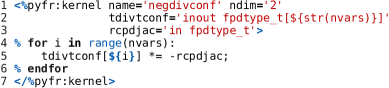
Figure 3: An example of an extrinsic kernel in PyFR. The template variable nvars is taken to be the number of field variables, $N_{v}$. The kernel arguments tdivtconf and rcpdjac correspond to $\tilde{\bm{\nabla}}\cdot\tilde{\mathbf{f}}$ and $J^{-1}$ respectively with the operation being performed in-place.

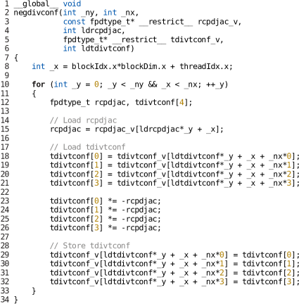
Figure 4: Generated CUDA source for the template in Figure 3 for when $N_{V}=4$.

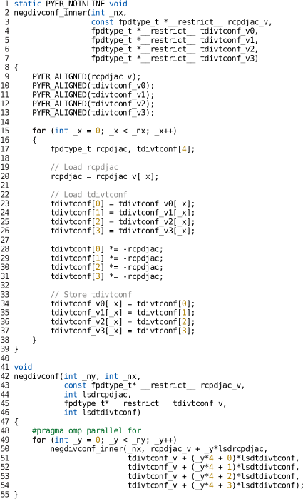
Figure 5: Generated OpenMP annotated C source code for the template in Figure 3 for when $N_{V}=4$. The somewhat unconventional structure is necessary to ensure that the kernel is properly vectorised across a range of compilers.

3.6 Distributed Memory Parallelism and Scheduling

PyFR is capable of operating on heigh performance computing clusters utilising distributed memory parallelism. This is accomplished through the Message Passing Interface (MPI). All MPI functionality is implemented at the Python level through the mpi4py [19] wrapper. To enhance the scalability of the code care has been taken to ensure that all requests are persistent, point-to-point and non-blocking. Further, the format of data that is shared between ranks has been made backend independent. It is therefore possible to deploy PyFR on heterogeneous clusters consisting of both conventional CPUs and accelerators.

The arrangement of kernel calls required to solve an advection-diffusion problem can be seen in Figure 6. Our primary objective when scheduling kernels was to maximise the potential for overlapping communication with computation. In order to help achieve this the common interface solution, $\mathfrak{C}_{\alpha}$, and common interface flux, $\mathfrak{F}_{\alpha}$, kernels have been broken apart into two separate kernels; suffixed in the figure by int and mpi. PyFR is therefore able to perform a significant degree of rank-local computation while the relevant ghost states are being exchanged.

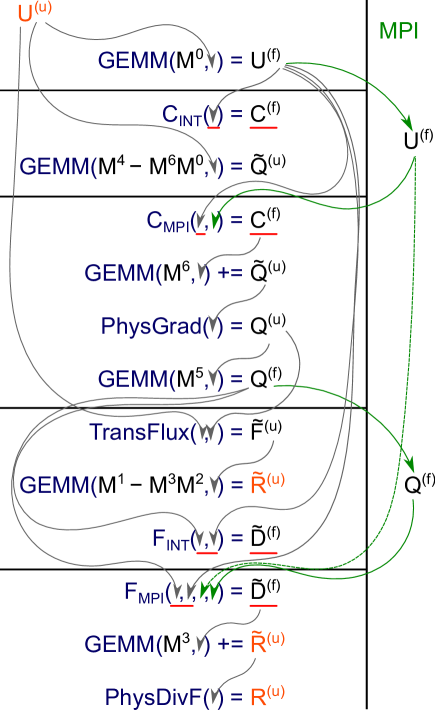
Figure 6: Flow diagram showing the stages required to compute $-\bm{\nabla}\cdot\mathbf{f}$. Symbols correspond to those of Appendix A. For simplicity arguments referencing constant data have been omitted. Memory indirection is indicated by red underlines. Synchronisation points are signified by black horizontal lines. Dotted lines correspond to data reuse.

Our secondary objective when scheduling kernels was to minimise the amount of temporary storage required during the evaluation of $-\bm{\nabla}\cdot\mathbf{f}$. Such optimisations are critical within the context of accelerators which often have an order of magnitude less memory than a contemporary platform. In order to help achieve this $\bm{\mathsf{U}}^{(u)}$, $\tilde{\bm{\mathsf{R}}}^{(u)}$, and $\bm{\mathsf{R}}^{(u)}$ are allowed to alias. By permitting the same storage location to be used for both the inputted solution and the outputted flux divergence it is possible to reduce the storage requirements of the RK schemes. Another opportunity for memory reuse is in the transformed flux function where the incoming gradients, $\bm{\mathsf{Q}}^{(u)}$, can be overwritten with the transformed flux, $\tilde{\bm{\mathsf{F}}}^{(u)}$. A similar approach can be used in the common interface flux function whereby $\bm{\mathsf{U}}^{(f)}$ can updated in-place with the entires of $\tilde{\bm{\mathsf{D}}}^{(f)}$ which holds the transformed common normal flux. Moreover, $\bm{\mathsf{C}}^{(f)}$ is also able to utilise the same storage as the somewhat larger $\bm{\mathsf{Q}}^{(f)}$ array. These optimisations allow PyFR to process over $100\,000$ curved, unstructured, hexahedral elements at $\wp=3$ inside of a $5\,\text{GiB}$ memory footprint.

4 Governing Systems

4.1 Overview

PyFR is a framework for solving various advection-diffusion type problems. In the current release of PyFR two specific governing systems can be solved, specifically the Euler equations for inviscid compressible flow, and the compressible Navier-Stokes equations for viscous compressible flow. Details regarding both are given below.

4.2 Euler Equations

Using the framework introduced in section 2 the three dimensional Euler equations can be expressed in conservative form as

$$u=\begin{Bmatrix}\rho\\ \rho v_{x}\\ \rho v_{y}\\ \rho v_{z}\\ E\end{Bmatrix},\qquad\mathbf{f}=\mathbf{f}^{(\mathrm{inv})}=\begin{Bmatrix}\rho v_{x}&\rho v_{y}&\rho v_{z}\\ \rho v_{x}^{2}+p&\rho v_{y}v_{x}&\rho v_{z}v_{x}\\ \rho v_{x}v_{y}&\rho v_{y}^{2}+p&\rho v_{z}v_{y}\\ \rho v_{x}v_{z}&\rho v_{y}v_{z}&\rho v_{z}^{2}+p\\ v_{x}(E+p)&v_{y}(E+p)&v_{z}(E+p)\end{Bmatrix},$$ (20)

with $u$ and $\mathbf{f}$ together satisfying Equation 1. In the above $\rho$ is the mass density of the fluid, $\mathbf{v}=(v_{x},v_{y},v_{z})^{T}$ is the fluid velocity vector, $E$ is the total energy per unit volume and $p$ is the pressure. For a perfect gas the pressure and total energy can be related by the ideal gas law

$$E=\frac{p}{\gamma-1}+\frac{1}{2}\rho\|\mathbf{v}\|^{2},$$ (21)

with $\gamma=C_{p}/C_{v}$.

With the fluxes specified all that remains is to prescribe a method for computing the common normal flux, $\mathfrak{F}_{\alpha}$, at interfaces as defined in Equation 15. This can be accomplished using an approximate Riemann solver for the Euler equations. There exist a variety of such solvers as detailed in [20]. A description of those implemented in PyFR can be found in Appendix B.

4.3 Compressible Navier-Stokes Equations

The compressible Navier-Stokes equations can be viewed as an extension of the Euler equations via the inclusion of viscous terms. Within the framework outlined above the flux now takes the form of $\mathbf{f}=\mathbf{f}^{(\text{inv})}-\mathbf{f}^{(\text{vis})}$ where

$$\mathbf{f}^{(\mathrm{vis})}=\begin{Bmatrix}0&0&0\\ \mathcal{T}_{xx}&\mathcal{T}_{yx}&\mathcal{T}_{zx}\\ \mathcal{T}_{xy}&\mathcal{T}_{yy}&\mathcal{T}_{zy}\\ \mathcal{T}_{xz}&\mathcal{T}_{yz}&\mathcal{T}_{zz}\\ v_{i}\mathcal{T}_{ix}+\Delta\partial_{x}T&v_{i}\mathcal{T}_{iy}+\Delta\partial_{y}T&v_{i}\mathcal{T}_{iz}+\Delta\partial_{z}T\end{Bmatrix}.$$ (22)

In the above we have defined $\Delta=\mu C_{p}/P_{r}$ where $\mu$ is the dynamic viscosity and $P_{r}$ is the Prandtl number. The components of the stress-energy tensor are given by

$$\mathcal{T}_{ij}=\mu(\partial_{i}v_{j}+\partial_{j}v_{i})-\frac{2}{3}\mu\delta_{ij}\bm{\nabla}\cdot\mathbf{v}.$$ (23)

Using the ideal gas law the temperature can be expressed as

$$T=\frac{1}{C_{v}}\frac{1}{\gamma-1}\frac{p}{\rho},$$ (24)

with partial derivatives thereof being given according to the quotient rule.

Since the Navier-Stokes equations are an advection-diffusion type system it is necessary to both compute a common solution ($\mathfrak{C}_{\alpha}$ of Equation 7) at element boundaries and augment the inviscid Riemann solver to handle the viscous part of the flux. A popular approach is the LDG method as presented in [5, 13]. In this approach the common solution is given $\forall\alpha$ according to

$$\mathfrak{C}(u_{L},u_{R})=(\tfrac{1}{2}-\beta)u_{L}+(\tfrac{1}{2}+\beta)u_{R},$$ (25)

where $\beta$ controls the degree of upwinding/downwinding. The common normal interface flux is then prescribed, once again $\forall\alpha$, according to

$$\mathfrak{F}(u_{L},u_{R},\mathbf{q}_{L},\mathbf{q}_{R},\hat{\mathbf{n}}_{L})=\mathfrak{F}^{(\text{inv})}-\mathfrak{F}^{(\text{vis})},$$ (26)

where $\mathfrak{F}^{(\text{inv})}$ is a suitable inviscid Riemann solver (see Appendix B) and

$$\mathfrak{F}^{(\text{vis})}=\hat{\mathbf{n}}^{\vphantom{(\text{vis})}}_{L}\cdot\left\{(\tfrac{1}{2}+\beta)\mathbf{f}^{(\text{vis})}_{L}+(\tfrac{1}{2}-\beta)\mathbf{f}^{(\text{vis})}_{R}\right\}+\tau(u_{L}^{\vphantom{(\text{vis})}}-u_{R}^{\vphantom{(\text{vis})}}),$$ (27)

with $\tau$ being a penalty parameter, $\mathbf{f}^{(\text{vis})}_{L}=\mathbf{f}^{(\text{vis})}_{\vphantom{L}}(u^{\vphantom{(\text{vis})}}_{L},\mathbf{q}^{\vphantom{(\text{vis})}}_{L})$, and $\mathbf{f}^{(\text{vis})}_{R}=\mathbf{f}^{(\text{vis})}_{\vphantom{R}}(u^{\vphantom{(\text{vis})}}_{R},\mathbf{q}^{\vphantom{(\text{vis})}}_{R})$. We observe here that if the common solution is upwinded then the common normal flux will be downwinded. Generally, $\beta=\pm 1/2$ as this results in the numerical scheme having a compact stencil and $0\leq\tau\leq 1$.

4.3.1 Presentation in Two Dimensions

The above prescriptions of the Euler and Navier-Stokes equations are valid for the case of $N_{D}=3$. The two dimensional formulation can be recovered by deleting the fourth rows in the definitions of $u$, $\mathbf{f}^{(\text{inv})}$ and $\mathbf{f}^{(\text{vis})}$ along with the third columns of $\mathbf{f}^{(\text{inv})}$ and $\mathbf{f}^{(\text{vis})}$. Vectors are now two dimensional with the velocity being given by $\mathbf{v}=(v_{x},v_{y})^{T}$.

5 Validation

5.1 Euler Equations: Euler Vortex Super Accuracy

Various authors [4, 10] have shown FR schemes exhibit so-called ‘super accuracy’ (an order of accuracy greater than the expected $\wp+1$). To confirm PyFR can achieve super accuracy for the Euler equations a square domain $\mathbf{\Omega}=[-20,20]^{2}$ was decomposed into four structured quad meshes with spacings of $h=1/3$, $h=2/7$, $h=1/4$, and $h=2/9$. Initial conditions were taken to be those of an isentropic Euler vortex in a free-stream

$$\rho(\mathbf{x},t=0) =\left\{1-\frac{S^{2}M^{2}(\gamma-1)\exp 2f}{8\pi^{2}}\right\}^{\frac{1}{\gamma-1}},$$ (28)

$$\mathbf{v}(\mathbf{x},t=0) =\frac{Sy\exp{f}}{2\pi R}\hat{\mathbf{x}}+\left\{1-\frac{Sx\exp{f}}{2\pi R}\right\}\hat{\mathbf{y}},$$ (29)

$$p(\mathbf{x},t=0) =\frac{\rho^{\gamma}}{\gamma M^{2}},$$ (30)

where $f=(1-x^{2}-y^{2})/2R^{2}$, $S=13.5$ is the strength of the vortex, $M=0.4$ is the free-stream Mach number, and $R=1.5$ is the radius. All meshes were configured with periodic boundary conditions along boundaries of constant $x$. Along boundaries of constant $y$ the dynamical variables were fixed according to

$$\rho(\mathbf{x}=x\hat{\mathbf{x}}\pm 20\hat{\mathbf{y}},t) =1,$$

$$\mathbf{v}(\mathbf{x}=x\hat{\mathbf{x}}\pm 20\hat{\mathbf{y}},t) =\hat{\mathbf{y}},$$

$$p(\mathbf{x}=x\hat{\mathbf{x}}\pm 20\hat{\mathbf{y}},t) =\frac{1}{\gamma M^{2}},$$

which are simply the limiting values of the initial conditions. Strictly speaking these conditions, on account of the periodicity, result in the modelling of an infinite array of coupled vortices. The impact of this is mitigated by the observation that the exponentially decaying vortex has a characteristic radius which is far smaller than the extent of the domain. Neglecting these effects the analytic solution of the system is a time $t$ is simply a translation of the initial conditions.

Using the analytical solution we can define an $L^{2}$ error as

$$\sigma(t)^{2}=\int_{-2}^{2}\int_{-2}^{2}\Bigl{[}\rho^{\delta}(\mathbf{x}+\Delta_{y}(t)\hat{\mathbf{y}},t)-\rho(\mathbf{x},t=0)\Bigr{]}^{2}\,\mathrm{d}^{2}\mathbf{x},$$ (31)

where $\rho^{\delta}(\mathbf{x},t)$ is the numerical mass density, $\rho(\mathbf{x},t=0)$ the analytic mass density, and $\Delta_{y}(t)$ is the ordinate corresponding to the centre of the vortex at a time $t$ and accounts for the fact that the vortex is translating in a free stream velocity of unity in the $y$ direction. Restricting the region of consideration to a small box centred around the origin serves to further mitigate against the effects of vortices coupling together. The initial mass density along with the $[-2,-2]\times[2,2]$ region used to evaluate the error can be seen in Figure 7. At times, $t_{c}$, when the vortex is centred on the box the error can be readily computed by integrating over each element inside the box and summing the residuals

$$\sigma(t_{c})^{2}=\iint_{\hat{\mathbf{\Omega}}_{e}}\Bigl{[}\rho^{\delta}_{i}(\tilde{\mathbf{x}},t_{c})-\rho(\bm{\mathcal{M}}_{i}(\tilde{\mathbf{x}}),0)\Bigr{]}^{2}J_{i}(\tilde{\mathbf{x}})\,\mathrm{d}^{2}\tilde{\mathbf{x}},$$ (32)

where, $\rho^{\delta}_{i}(\tilde{\mathbf{x}},t_{c})$ is the approximate mass density inside of the $i$th element, and $J_{i}(\tilde{\mathbf{x}})$ the associated Jacobian. These integrals can be approximated by applying Gaussian quadrature

$$\sigma(t_{c})^{2} \approx J_{i}(\tilde{\mathbf{x}}_{j})\Bigl{[}\rho^{\delta}_{i}(\tilde{\mathbf{x}}_{j},t_{c})-\rho(\bm{\mathcal{M}}_{i}(\tilde{\mathbf{x}}_{j}),0)\Bigr{]}^{2}\omega_{j}$$ (33)

$$=\frac{h^{2}}{4}\Bigl{[}\rho^{\delta}_{i}(\tilde{\mathbf{x}}_{j},t_{c})-\rho(\bm{\mathcal{M}}_{i}(\tilde{\mathbf{x}}_{j}),0)\Bigr{]}^{2}\omega_{j},$$

where $\set{\tilde{\mathbf{x}}_{j}}$ are abscissa and $\set{\omega_{j}}$ the weights of a rule determined for integration inside of a standard quadrilateral. So long as the rule used is of a suitable strength then this will be a very good approximation of the true $L^{2}$ error.

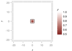
Figure 7: Initial density profile for the vortex in $\mathbf{\Omega}$. The black box shows the region where the error is calculated.

Following [10] the initial conditions were laid onto the mesh using a collocation projection with $\wp=3$. The simulation was then run with three different flux reconstruction schemes: DG, SD, and HU as defined in [10]. Solution points were placed at a tensor product construction of Gauss-Legendre quadrature points. Common interface fluxes were computed using a Rusanov Riemann solver. To advance the solutions in time a classical fourth order Runge-Kutta method (RK4) was used. The time step was taken to be $\Delta t=0.00125$ with $t=0..1800$ with solutions written out to disk every $32\,000$ steps. The order of accuracy of the scheme at a particular time can be determined by plotting $\log\sigma$ against $\log h$ and performing a least-squares fit through the four data points. The order is given by the gradient of the fit. A plot of order of accuracy against time for the three schemes can be seen in Figure 8. We note that the order of accuracy changes as a function of time. This is due to the fact that the error is actually of the form $\sigma(t)=\sigma_{\text{p}}+\sigma_{\text{so}}(t)$ where $\sigma_{\text{p}}$ is a constant projection error and $\sigma_{\text{so}}$ is a time-dependent spatial operator error. The projection error arises as a consequence of the forth order collocation projection of the initial conditions onto the mesh. Over time the spatial operator error grows in magnitude and eventually dominates. Only when $\sigma_{\text{so}}(t)\gg\sigma_{\text{p}}$ can the true order of the method be observed. The results here can be seen to be in excellent agreement with those of [10].

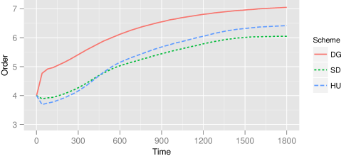
Figure 8: Spatial super accuracy observed for a $\wp=3$ simulation using DG, SD and HU as defined in [10].

5.2 Compressible Navier-Stokes Equations: Couette Flow

Consider the case in which two parallel plates of infinite extent are separated by a distance $H$ in the $y$ direction. We treat both plates as isothermal walls at a temperature $T_{w}$ and permit the top plate to move at a velocity $v_{w}$ in the $x$ direction with respect to the bottom plate. For simplicity we shall take the ordinate of the bottom plate as zero. In the case of a constant viscosity $\mu$ the Navier-Stokes equations admit an analytical solution in which

$$\rho(\phi) =\frac{\gamma}{\gamma-1}\frac{2p}{2C_{p}T_{w}+P_{r}v_{w}^{2}\phi(1-\phi)},$$ (34)

$$\mathbf{v}(\phi) =v_{w}\phi\hat{\mathbf{x}},$$ (35)

$$p =p_{c},$$ (36)

where $\phi=y/H$ and $p_{c}$ is a constant pressure. The total energy is given by the ideal gas law of Equation 21. On a finite domain the Couette flow problem can be modelled through the imposition of periodic boundary conditions. For a two dimensional mesh periodicity is enforced in $x$ whereas for three dimensional meshes it is enforced in both $x$ and $z$. To validate the Navier-Stokes solver in PyFR we take $\gamma=1.4$, $P_{r}=0.72$, $\mu=0.417$, $C_{p}=$1005\text{\,}\mathrm{J}\text{\,}{\mathrm{K}}^{-1}$$, $H=$1\text{\,}\mathrm{m}$$, $T_{w}=$300\text{\,}\mathrm{K}$$, $p_{c}=$1\text{\times}{10}^{5}\text{\,}\mathrm{Pa}$$, and $v_{w}=$69.445\text{\,}\mathrm{m}\text{\,}{\mathrm{s}}^{-1}$$. These values correspond to a Mach number of 0.2 and a Reynolds number of 200. The plates were modelled as no-slip isothermal walls as detailed in subsection C.4 of Appendix C. A plot of the resulting energy profile can be seen in Figure 9. Constant initial conditions are taken as $\rho=\big{\langle}\,\rho(\phi)\,\big{\rangle}$, $\mathbf{v}=v_{w}\hat{\mathbf{x}}$, and $p=p_{c}$. Using the analytical solution we again define an $L^{2}$ error as

$$\sigma(t)^{2} =\int_{\mathbf{\Omega}}\left[E^{\delta}(\mathbf{x},t)-E(\mathbf{x})\right]^{2}\,\mathrm{d}^{N_{D}}\mathbf{x}$$ (37)

$$=\int_{\mathbf{\Omega}_{ei}}\left[E^{\delta}_{ei}(\tilde{\mathbf{x}},t)-E(\bm{\mathcal{M}}_{ei}(\tilde{\mathbf{x}}))\right]^{2}J_{ei}(\tilde{\mathbf{x}})\,\mathrm{d}^{N_{D}}\tilde{\mathbf{x}}$$ (38)

$$\approx\left[E^{\delta}_{ei}(\tilde{\mathbf{x}}_{ej},t)-E(\bm{\mathcal{M}}_{ei}(\tilde{\mathbf{x}}_{ej}))\right]^{2}J_{ei}(\tilde{\mathbf{x}}_{ej})\omega_{ej},$$ (39)

where $\mathbf{\Omega}$ is the computational domain, $E^{\delta}(\mathbf{x},t)$ is the numerical total energy, and $E(\mathbf{x})$ the analytic total energy. In the third step we have approximated each integral by a quadrature rule with abscissa $\set{\tilde{\mathbf{x}}_{ej}}$ and weights $\set{\omega_{ej}}$ inside of an element type $e$. Couette flow is a steady state problem and so in the limit of $t\rightarrow\infty$ the numerical total energy should converge to a solution. Starting from a constant initial condition the $L^{2}$ error was computed every $0.1$ time units. The simulation was said to have converged when $\sigma(t)/\sigma(t+0.1)\leq 1.01$ where $\sigma$ is the $L^{2}$ error. We will denote the time at which this occurs by $t_{\infty}$.

Once the system has converged for a range of meshes it is possible to compute the order of accuracy of the scheme. For a given $\wp$ this is the slope (plus or minus a standard error) of a linear least squares fit of $\log h\sim\log\sigma(t_{\infty})$ where $h$ is an approximation of the characteristic grid spacing. The expected order of accuracy is $\wp+1$. In all simulations inviscid fluxes were computed using the Rusanov approach and the LDG parameters were taken to be $\beta=1/2$ and $\tau=0.1$. All simulations were performed with DG correction functions and at double precision. Inside tensor product elements Gauss-Legendre solution and flux points were employed. Triangular elements utilised Williams-Shunn solution points and Gauss-Legendre flux points.

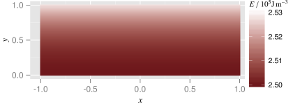
Figure 9: Converged steady state energy profile for the two dimensional Couette flow problem.

Two dimensional unstructured mixed mesh.

For the two dimensional test cases the computational domain was taken to be $[-1,1]\times[0,1]$. This domain was then meshed with both triangles and quadrilaterals at four different refinement levels. The Couette flow problem described above was then solved on each of these meshes. Experimental $L^{2}$ errors and orders of accuracy can be seen in Table 2. We note that in all cases the expected order of accuracy was obtained.

(a)

(b)

(c)

(d)

Figure 10: Unstructured mixed element meshes used for the two dimensional Couette flow problem.

Table 2: $L^{2}$ energy error and orders of accuracy for the Couette flow problem on four mixed meshes. The mesh spacing was approximated as $h\sim N_{E}^{-1/2}$ where $N_{E}$ is the total number of elements in the mesh.

		$\sigma(t_{\infty})\,/\,$\mathrm{J}\text{\,}{\mathrm{m}}^{-3}$$
Tris	Quads	$\wp=1$	$\wp=2$	$\wp=3$	$\wp=4$
2	8	$1.26\times 10^{2}$	$5.77\times 10^{-1}$	$5.54\times 10^{-3}$	$6.62\times 10^{-5}$
6	22	$3.56\times 10^{1}$	$1.40\times 10^{-1}$	$6.72\times 10^{-4}$	$3.91\times 10^{-6}$
10	37	$2.08\times 10^{1}$	$4.35\times 10^{-2}$	$2.54\times 10^{-4}$	$8.16\times 10^{-7}$
16	56	$1.46\times 10^{1}$	$3.52\times 10^{-2}$	$1.09\times 10^{-4}$	$4.62\times 10^{-7}$
Order		$2.21\pm 0.12$	$2.99\pm 0.32$	$3.97\pm 0.05$	$5.20\pm 0.38$

Three dimensional extruded hexahedral mesh.

For this three dimensional case the computational domain was taken to be $[-1,1]\times[0,1]\times[0,1]$. Meshes were constructed through first generating a series of unstructured quadrilateral meshes in the $x$-$y$ plane. A three layer extrusion was then performed on this meshes to yield a series of hexahedral meshes. Experimental $L^{2}$ errors and orders of accuracy for these meshes can be seen in Table 3.

Table 3: $L^{2}$ energy errors and orders of accuracy for the Couette flow problem on three extruded hexahedral meshes. On account of the extrusion $h\sim N^{-1/2}_{E}$ where $N_{E}$ is the total number of elements in the mesh.

	$\sigma(t_{\infty})\,/\,$\mathrm{J}\text{\,}{\mathrm{m}}^{-3}$$
Hexes	$\wp=1$	$\wp=2$	$\wp=3$
78	$3.35\times 10^{1}$	$5.91\times 10^{-2}$	$7.28\times 10^{-4}$
195	$1.23\times 10^{1}$	$1.87\times 10^{-2}$	$1.15\times 10^{-4}$
405	$6.15\times 10^{0}$	$5.49\times 10^{-3}$	$2.72\times 10^{-5}$
Order	$2.06\pm 0.08$	$2.87\pm 0.24$	$3.99\pm 0.03$

Three dimensional unstructured hexahedral mesh.

As a further test a domain of dimension $[0,1]^{3}$ was considered. This domain was meshed using completely unstructured hexahedra. Three levels of refinement were used resulting in meshes with 96, 536 and 1004 elements. A cutaway of the most refined mesh can be seen in Figure 11. Experimental $L^{2}$ errors and the resulting orders of accuracy are presented in Table 4. Despite the fully unstructured nature of the mesh the expected order of accuracy was again obtained in all cases. We do, however, note the higher standard errors associated with these results.

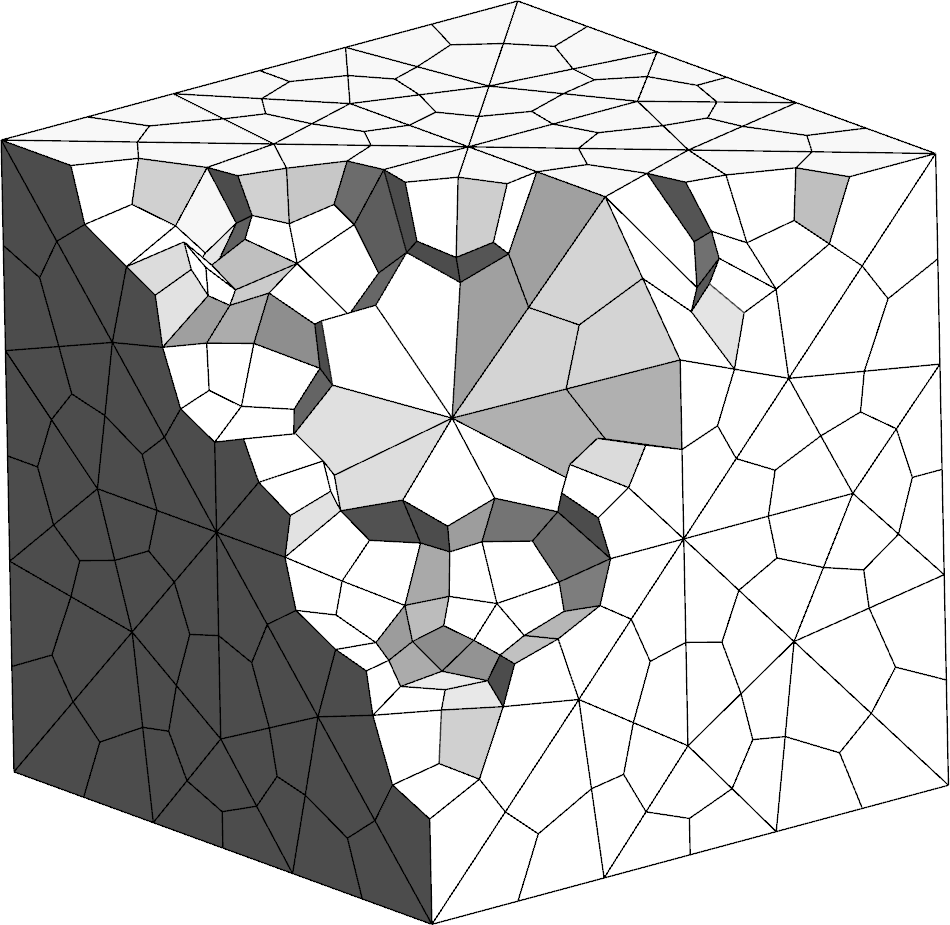
Figure 11: Cutaway of the unstructured hexahedral mesh with 1004 elements.

Table 4: $L^{2}$ energy errors and orders of accuracy for the Couette flow problem on three unstructured hexahedral meshes. Mesh spacing was taken as $h\sim N^{-1/3}_{E}$ where $N_{E}$ is the total number of elements in the mesh.

	$\sigma(t_{\infty})\,/\,$\mathrm{J}\text{\,}{\mathrm{m}}^{-3}$$
Hexes	$\wp=1$	$\wp=2$	$\wp=3$
96	$1.91\times 10^{1}$	$4.32\times 10^{-2}$	$5.83\times 10^{-4}$
536	$8.20\times 10^{0}$	$9.11\times 10^{-3}$	$6.89\times 10^{-5}$
1004	$3.82\times 10^{0}$	$3.22\times 10^{-3}$	$2.04\times 10^{-5}$
Order	$1.93\pm 0.46$	$3.19\pm 0.48$	$4.16\pm 0.44$

5.3 Compressible Navier-Stokes Equations: Flow Over a Cylinder

In order to demonstrate the ability of PyFR to solve the unsteady Navier-Stokes equations flow over a cylinder at Reynolds number 3900 and Mach number $M=0.2$ was simulated. A cylinder of radius $1/2$ was placed at $(0,0)$ inside of a domain of dimension $[-18,30]\times[-10,10]\times[0,3.2]$. This domain was then meshed in the $x$-$y$ plane with 4661 quadratically curved quadrilateral elements. Next, this grid was extruded along the $z$-axis to yield a total of 46610 hexahedra. The grid, which can be seen in Figure 12, was partitioned into four pieces. Along surfaces of $y=\pm 10$ and $x=-18$ the inflow boundary condition of subsection C.2 in Appendix C was imposed. Along the surface of $x=30$ the outflow condition of subsection C.3 in Appendix C was used. Periodic conditions were imposed in the $z$ direction. On the surface of the cylinder the no-slip isothermal wall condition of subsection C.4 in Appendix C was imposed. The free-stream conditions were taken to be $\rho=1$, $\mathbf{v}=\hat{\mathbf{x}}$, and $p=1/\gamma M^{2}$. These were also used as the initial conditions for the simulation. DG correction functions were used with the LDG parameters being $\beta=1/2$ and $\tau=0.1$. The ratio of specific heats was taken as $\gamma=1.4$ and the Prandtl number as $P_{r}=0.72$.

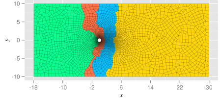
Figure 12: Cross section in the $x$-$y$ plane of the cylinder mesh. Colours indicate the partition to which the elements belong.

The simulation was run with $\wp=4$ with four NVIDIA K20c GPUs. It contained some $29\times 10^{6}$ degrees of freedom. Isosurfaces of density captured after the turbulent wake had fully developed can be seen in Figure 13.

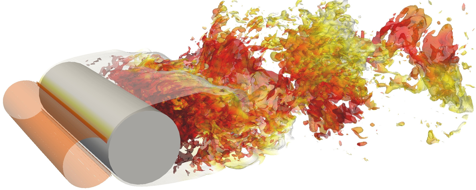
Figure 13: Isosurfaces of density around the cylinder.

6 Single Node Performance

The single node performance of PyFR has been evaluated on an NVIDIA M2090 GPU. This accelerator has a theoretical peak double precision floating point performance of $665\,\text{GFLOP/s}$, and when ECC is disabled the theoretical peak memory bandwidth is $177\,\text{GB/s}$. As points of reference we observe that cuBLAS (CUDA 5.5) is able to obtain $407\,\text{GFLOP/s}$ when multiplying a pair of $4096\times 4096$ matrices on this hardware, and the maximum device bandwidth obtainable by the bandwidth test application included with the CUDA SDK is $138.9\,\text{GiB/s}$ when ECC is disabled. We shall refer to these values as realisable peaks.

To conduct the evaluation a fully periodic cuboidal domain was meshed with $50\,176$ hexahedral elements. The double precision Navier-Stokes solver of PyFR was then run on this mesh at orders $\wp=2,3,4$ with $\beta=1/2$. In conducting the analysis kernels were grouped into one of three categories: matrix multiplications (DGEMM), point-wise kernels with direct memory access patterns (PD) and point-wise kernels with some level of indirect memory access (PI). Indirection arises in the computation of $\mathfrak{C}_{\alpha}$ in Equation 7 and $\mathfrak{F}_{\alpha}$ in Equation 15 and occurs as a consequence of the unstructured nature of PyFR. The resulting breakdowns of wall-clock time, memory bandwidth and floating point operations can be seen in Table 5. It is clear that he majority of floating point operations are concentrated inside the calls to DGEMM with the point-wise operations are heavily memory bandwidth bound. Of this bandwidth some ${\sim}15\%$ was ascribed to register spillage above and beyond that which can be absorbed by the L1 cache.

Table 5: Single GPU performance of PyFR for the Navier-Stokes equations when run on an NVIDIA M2090 with ECC disabled. As the memory bandwidth requirements of DGEMM are dependent on the accumulation strategy adopted by the implementation these values have been omitted.

		Order
		$\wp=2$	$\wp=3$	$\wp=4$
Wall time / %
	DGEMM	$55.7$	$66.2$	$81.4$
	PD	$24.9$	$21.5$	$12.8$
	PI	$19.4$	$12.3$	$5.8$
Bandwidth / GiB/s
	PD	$125.5$	$125.0$	$124.8$
	PI	$124.8$	$124.3$	$124.2$
Arithmetic / GFLOP/s
	DGEMM	$205.3$	$368.1$	$305.4$
	PD	$0.7$	$0.7$	$0.7$
	PI	$0.9$	$0.8$	$0.9$

The high fraction of peak bandwidth obtained by the indirect kernels can be attributed to three factors. Firstly, the constant data required for calculations at ????, such as $\hat{\mathbf{n}}^{(f)}_{e\sigma n}$ and $J^{(f)}_{e\sigma n}n^{(f)}_{e\sigma n}$, is ordered to ensure direct (coalesced) access. Secondly, at start-up PyFR attempts to determine an iteration ordering over the various flux-point pairs that will minimise the number of cache misses.

Many of the memory accesses are therefore are near-coalesced. Thirdly and finally we highlight the impressive latency-hiding capabilities of the CUDA programming model.

In line with expectations the proportion of time spent performing matrix-matrix multiplications increases as a function of order. When going from $\wp=2$ to $\wp=3$ a significant portion of the additional compute is offset by the improved performance of cuBLAS. However, when $\wp=4$ the performance of these kernels in absolute terms can be seen to regress slightly. This contributes to the greatly increased fraction of wall-clock time spent inside of these kernels. Nevertheless, the achieved rate of $305.4\text{GFLOP/s}$ is still over $75\%$ of the realisable peak. Also in line with expectations is the invariance of the arithmetic performance of the point-wise kernels with respect to order. As the order is varied all that changes is the number of points to be processed with the operation itself remaining identical.

7 Scalability

The scalability of PyFR has been evaluated on the Emerald GPU cluster. It is housed at the STFC Rutherford Appleton Laboratory and based around 60 HP SL390 nodes with three NVIDIA M2090 GPUs and 24 HP SL390 nodes with eight NVIDIA M2090 GPUs. Nodes are connected by QDR InfiniBand.

For simplicity all runs herein were performed on the eight GPU nodes. As a starting point a domain of dimension $[-16,16]\times[-16,16]\times[0,1.75]$ was meshed isotropically with $N_{E}=114\,688$ structured hexahedral elements. The mesh was configured with completely periodic boundary conditions. When run with the Navier-Stokes solver in PyFR with $\wp=3$ the mesh gives a working set of ${\sim}4720\,\text{MiB}$. This is sufficient to 90% load an M2090 which when ECC is enabled has ${\sim}5250\,\text{MiB}$ memory available to the user. When examining the scalability of a code there are two commonly used metrics. The first of these is weak scalability in which the size of the target problem is increased in proportion to the number of ranks $N$ with $N_{E}\propto N$. For a code with perfect weak scalability the runtime should remain unchanged as more ranks are added. The second metric is strong scalability wherein the problem size is fixed and the speedup compared to a single rank is assessed. Perfect strong scalability implies that the runtime scales as $1/N$.

For the domain outlined above weak scalability was evaluated by increasing the dimensions of the domain according to $[-16,16]\times N[-16,16]\times[0,1.75]$. This extension permitted the domain to be trivially decomposed along the $y$-axis. The resulting runtimes for $1\leq N\leq 104$ can be seen in Table 6. We note that in the $N=104$ case that the simulation consisted of some $3.8\times 10^{9}$ degrees of freedom with a working set of ${\sim}485\,\text{GiB}$.

Table 6: Weak scalability of PyFR for the Navier-Stokes equations with $\wp=3$. Runtime is normalised with respect to a single NVIDIA M2090 GPU.

# M2090s	1	2	4	8	16	32	64	104
Runtime	1.00	1.00	1.01	1.01	1.01	1.01	1.01	1.01

To study the strong scalability the initial domain was partitioned along the $x$- and $y$-axes. Each partition contained exactly $N_{E}/N$s. The resulting speedups for $1\leq N\leq 32$ can be seen in Table 7. Up to eight GPUs scalability can be seen to be near perfect. Beyond this the relationship begins to break down. When $N=32$ an improvement of 26 can be observed. However, in this case each GPU is loaded to less than 3% and so the result is to be expected.

Table 7: Strong scalability of PyFR for the Navier-Stokes equations with $\wp=3$. The speedup is relative to a single NVIDIA M2090 GPU.

# M2090s	1	2	4	8	16	32
Speedup	1.00	2.03	3.96	7.48	14.07	26.18

8 Conclusions

In this paper we have described PyFR, an open source Python based framework for solving advection-diffusion type problems on streaming architectures. The structure and ethos of PyFR has been explained including our methodology for targeting multiple hardware platforms. We have shown that PyFR exhibits spatial super accuracy when solving the 2D Euler equations and the expected order of accuracy when solving Couette flow problem on a range of grids in 2D and 3D. Qualitative results for unsteady 3D viscous flow problems on curved grids have also been presented. Performance of PyFR has been validated on an NVIDIA M2090 GPU in three dimensions. It has been shown that the compute bound kernels are able to obtain between $50\%$ and $90\%$ of realisable peak FLOP/s whereas the bandwidth bound point-wise kernels are, across the board, able to obtain in excess of $89\%$ realisable peak bandwidth. The scalability of PyFR has been demonstrated in the strong sense up to 32 NVIDIA M2090s and in the weak sense up to 104 NVIDIA M2090s when solving the 3D Navier-Stokes equations.

Appendix A Matrix Representation

It is possible to cast the majority of operations in an FR step as matrix-matrix multiplications of the form

$$\bm{\mathsf{C}}\leftarrow c_{1}\bm{\mathsf{A}}\bm{\mathsf{B}}+c_{2}\bm{\mathsf{C}},$$ (40)

where $c_{1,2}\in\mathbb{R}$ are constants, $\bm{\mathsf{A}}$ is a constant operator matrix, and $\bm{\mathsf{B}}$ and $\bm{\mathsf{C}}$ are state matrices. To accomplish this we start by introducing the following constant operator matrix

$$\big{(}\bm{\mathsf{M}}^{0}_{e}\big{)}_{\sigma\rho} =\ell^{(u)}_{e\rho}(\tilde{\mathbf{x}}^{(f)}_{e\sigma}), \dim\bm{\mathsf{M}}^{0}_{e} =N_{e}^{(f)}\times N_{e}^{(u)},$$

and the following state matrices

$$\big{(}\bm{\mathsf{U}}^{(u)}_{e}\big{)}_{\rho(n\alpha)} =u^{(u)}_{e\rho n\alpha}, \dim\bm{\mathsf{U}}^{(u)}_{e} =N_{e}^{(u)}\times N_{V}|\mathbf{\Omega}_{e}|,$$

$$\big{(}\bm{\mathsf{U}}^{(f)}_{e}\big{)}_{\sigma(n\alpha)} =u^{(f)}_{e\sigma n\alpha}, \dim\bm{\mathsf{U}}^{(f)}_{e} =N_{e}^{(f)}\times N_{V}|\mathbf{\Omega}_{e}|.$$

In specifying the state matrices there is a degree of freedom associated with how the $N_{V}$ field variables for each element are packed along a row of the matrix, with the possible packing choices being discussed in subsection 3.3. Using these matrices we are able to reformulate Equation 6 as

$$\bm{\mathsf{U}}^{(f)}_{e}=\bm{\mathsf{M}}^{0}_{e}\bm{\mathsf{U}}^{(u)}_{e}.$$ (41)

In order to apply a similar procedure to Equation 9 we let

$$\big{(}\bm{\mathsf{M}}^{4}_{e}\big{)}_{\rho\sigma} =\big{[}\tilde{\bm{\nabla}}\ell^{(u)}_{e\rho}(\tilde{\mathbf{x}})\big{]}_{\tilde{\mathbf{x}}=\tilde{\mathbf{x}}^{(u)}_{e\sigma}}, \dim\bm{\mathsf{M}}^{4}_{e}, =N_{D}N_{e}^{(u)}\times N_{e}^{(u)},$$

$$\big{(}\bm{\mathsf{M}}^{6}_{e}\big{)}_{\rho\sigma} =\big{[}\hat{\tilde{\mathbf{n}}}^{(f)}_{e\rho}\cdot\tilde{\bm{\nabla}}\cdot\mathbf{g}^{(f)}_{e\rho}(\tilde{\mathbf{x}})\big{]}_{\tilde{\mathbf{x}}=\tilde{\mathbf{x}}^{(f)}_{e\sigma}}, \dim\bm{\mathsf{M}}^{6}_{e}, =N_{D}N_{e}^{(u)}\times N_{e}^{f},$$

$$\big{(}\bm{\mathsf{C}}^{(f)}_{e}\big{)}_{\rho(n\alpha)} =\mathfrak{C}_{\alpha}u^{(f)}_{e\rho n\alpha}, \dim\bm{\mathsf{C}}^{(f)}_{e} =N^{(f)}_{e}\times N_{V}\left\lvert\mathbf{\Omega}_{e}\right\rvert,$$

$$\big{(}\tilde{\bm{\mathsf{Q}}}^{(u)}_{e}\big{)}_{\sigma(n\alpha)} =\tilde{\mathbf{q}}^{(u)}_{e\sigma n\alpha}, \dim\tilde{\bm{\mathsf{Q}}}^{(u)}_{e} =N_{D}N^{(u)}_{e}\times N_{V}\left\lvert\mathbf{\Omega}_{e}\right\rvert,$$

Here it is important to qualify assignments of the form $\bm{\mathsf{A}}_{ij}=\mathbf{x}$ where $\mathbf{x}$ is a $N_{D}$ component vector. As above there is a degree of freedom associated with the packing. With the benefit of foresight we take the stride between subsequent elements of $\mathbf{x}$ in a matrix column to be either $\Delta i=N^{(u)}_{e}$ or $\Delta i=N^{(f)}_{e}$ depending on the context. With these matrices Equation 9 reduces to

$$\tilde{\bm{\mathsf{Q}}}^{(u)}_{e} =\bm{\mathsf{M}}^{6}_{e}\big{\{}\bm{\mathsf{C}}^{(f)}_{e}-\bm{\mathsf{U}}^{(f)}_{e}\big{\}}+\bm{\mathsf{M}}^{4}_{e}\bm{\mathsf{U}}^{(u)}_{e}$$ (42)

$$=\bm{\mathsf{M}}^{6}_{e}\big{\{}\bm{\mathsf{C}}^{(f)}_{e}-\bm{\mathsf{M}}^{0}_{e}\bm{\mathsf{U}}^{(u)}_{e}\big{\}}+\bm{\mathsf{M}}^{4}_{e}\bm{\mathsf{U}}^{(u)}_{e}$$

$$=\bm{\mathsf{M}}^{6}_{e}\bm{\mathsf{C}}^{(f)}_{e}+\big{\{}\bm{\mathsf{M}}^{4}_{e}-\bm{\mathsf{M}}^{6}_{e}\bm{\mathsf{M}}^{0}_{e}\big{\}}\bm{\mathsf{U}}^{(u)}_{e}.$$

Applying the procedure to Equation 11 we take

$$\bm{\mathsf{M}}^{5}_{e} =\operatorname{diag}(\bm{\mathsf{M}}^{0}_{e},\ldots,\bm{\mathsf{M}}^{0}_{e}) \dim{\bm{\mathsf{M}}^{5}_{e}} =N_{D}N^{(f)}_{e}\times N_{D}N^{(u)}_{e},$$

$$\big{(}\bm{\mathsf{Q}}^{(u)}_{e}\big{)}_{\sigma(n\alpha)} =\mathbf{q}^{(u)}_{e\sigma n\alpha}, \dim{\bm{\mathsf{Q}}^{(u)}_{e}} =N_{D}N^{(u)}_{e}\times N_{V}\left\lvert\mathbf{\Omega}_{e}\right\rvert,$$

$$\big{(}\bm{\mathsf{Q}}^{(f)}_{e}\big{)}_{\sigma(n\alpha)} =\mathbf{q}^{(f)}_{e\sigma n\alpha}, \dim{\bm{\mathsf{Q}}^{(f)}_{e}} =N_{D}N^{(f)}_{e}\times N_{V}\left\lvert\mathbf{\Omega}_{e}\right\rvert,$$

hence

$$\bm{\mathsf{Q}}^{(f)}_{e}=\bm{\mathsf{M}}^{5}_{e}\bm{\mathsf{Q}}^{(u)}_{e},$$ (43)

where we note the block diagonal structure of $\bm{\mathsf{M}}^{5}_{e}$. This is a direct consequence of the above choices for $\Delta i$. Finally, to rewrite Equation 18 we write

$$\big{(}\bm{\mathsf{M}}^{1}_{e}\big{)}_{\rho\sigma} =\big{[}\tilde{\bm{\nabla}}\ell^{(u)}_{e\rho}(\tilde{\mathbf{x}})\big{]}^{T}_{\tilde{\mathbf{x}}=\tilde{\mathbf{x}}^{(u)}_{e\sigma}}, \dim\bm{\mathsf{M}}^{1}_{e} =N^{(u)}_{e}\times N_{D}N^{(u)}_{e},$$

$$\big{(}\bm{\mathsf{M}}^{2}_{e}\big{)}_{\rho\sigma} =\big{[}\ell^{(u)}_{e\rho}(\tilde{\mathbf{x}}^{(f)}_{e\sigma})\hat{\tilde{\mathbf{n}}}^{(f)}_{e\sigma}\big{]}^{T}, \dim\bm{\mathsf{M}}^{2}_{e} =N^{(f)}_{e}\times N_{D}N^{(u)}_{e},$$

$$\big{(}\bm{\mathsf{M}}^{3}_{e}\big{)}_{\rho\sigma} =\big{[}\tilde{\bm{\nabla}}\cdot\mathbf{g}^{(f)}_{e\sigma}(\tilde{\mathbf{x}})\big{]}_{\tilde{\mathbf{x}}=\tilde{\mathbf{x}}^{(u)}_{e\rho}}, \dim\bm{\mathsf{M}}^{3}_{e} =N^{(u)}_{e}\times N^{(f)}_{e},$$

$$\big{(}\tilde{\bm{\mathsf{D}}}^{(f)}_{e}\big{)}_{\sigma(n\alpha)} =\mathfrak{F}^{\vphantom{(f_{\perp})}}_{\alpha}\tilde{f}^{(f_{\perp})}_{e\sigma n\alpha}, \dim\tilde{\bm{\mathsf{D}}}^{(f)}_{e} =N^{(f)}_{e}\times N_{V}\left\lvert\mathbf{\Omega}_{e}\right\rvert,$$

$$\big{(}\tilde{\bm{\mathsf{F}}}^{(u)}_{e}\big{)}_{\rho(n\alpha)} =\tilde{\mathbf{f}}^{(u)}_{e\rho n\alpha}, \dim\tilde{\bm{\mathsf{F}}}^{(u)}_{e} =N_{D}N^{(u)}_{e}\times N_{V}\left\lvert\mathbf{\Omega}_{e}\right\rvert,$$

$$\big{(}\tilde{\bm{\mathsf{R}}}^{(u)}_{e}\big{)}_{\rho(n\alpha)} =(\tilde{\bm{\nabla}}\cdot\tilde{\mathbf{f}})^{(u)}_{e\rho n\alpha}, \dim\tilde{\bm{\mathsf{R}}}^{(u)}_{e} =N_{e}^{(u)}\times N_{V}\left\lvert\mathbf{\Omega}_{e}\right\rvert,$$

and after substitution of Equation 13 for $\tilde{f}^{(f_{\perp})}_{e\sigma n\alpha}$ obtain

$$\tilde{\bm{\mathsf{R}}}^{(u)}_{e} =\bm{\mathsf{M}}^{3}_{e}\big{\{}\tilde{\bm{\mathsf{D}}}^{(f)}_{e}-\bm{\mathsf{M}}^{2}_{e}\tilde{\bm{\mathsf{F}}}^{(u)}_{e}\big{\}}+\bm{\mathsf{M}}^{1}_{e}\tilde{\bm{\mathsf{F}}}^{(u)}_{e}$$ (44)

$$=\bm{\mathsf{M}}^{3}_{e}\tilde{\bm{\mathsf{D}}}^{(f)}_{e}+\big{\{}\bm{\mathsf{M}}^{1}_{e}-\bm{\mathsf{M}}^{3}_{e}\bm{\mathsf{M}}^{2}_{e}\big{\}}\tilde{\bm{\mathsf{F}}}^{(u)}_{e}.$$

Appendix B Approximate Riemann Solvers

B.1 Overview

In the following section we take $u_{L}$ and $u_{R}$ to be the two discontinuous solution states at an interface and $\hat{\mathbf{n}}_{L}$ to be the normal vector associated with the first state. For convenience we take $\mathbf{f}^{(\text{inv})}_{L}=\mathbf{f}^{(\text{inv})}_{\vphantom{L}}(u^{\vphantom{(\text{inv})}}_{L})$, and $\mathbf{f}^{(\text{inv})}_{R}=\mathbf{f}^{(\text{inv})}_{\vphantom{R}}(u^{\vphantom{(\text{inv})}}_{R})$ with inviscid fluxes being prescribed by Equation 20.

B.2 Rusanov

Also known as the local Lax-Friedrichs method a Rusanov type Riemann solver imposes inviscid numerical interface fluxes according to

$$\mathfrak{F}^{(\text{inv})}=\frac{\hat{\mathbf{n}}_{L}}{2}\cdot\left\{\mathbf{f}^{(\text{inv})}_{L}+\mathbf{f}^{(\text{inv})}_{R}\right\}+\frac{s}{2}(u_{L}-u_{R}),$$ (45)

where $s$ is an estimate of the maximum wave speed

$$s=\sqrt{\frac{\gamma(p_{L}+p_{R})}{\rho_{L}+\rho_{R}}}+\frac{1}{2}\big{|}\hat{\mathbf{n}}_{L}\cdot(\mathbf{v}_{L}+\mathbf{v}_{R})\big{|}.$$ (46)

Appendix C Boundary Conditions

C.1 Overview

To incorporate boundary conditions into the FR approach we introduce a set of boundary interface types $b\in\mathcal{B}$. At a boundary interface there is only a single flux point: that which belongs to the element whose edge/face is on the boundary. Associated with each boundary type are a pair of functions $\mathfrak{C}^{(b)}_{\alpha}(u_{L})$ and $\mathfrak{F}^{(b)}_{\alpha}(u_{L},\mathbf{q}_{L},\hat{\mathbf{n}}_{L})$ where $u_{L}$, $\mathbf{q}_{L}$, and $\hat{\mathbf{n}}_{L}$ are the solution, solution gradient and unit normals at the relevant flux point. These functions prescribe the common solutions and normal fluxes, respectively.

Instead of directly imposing solutions and normal fluxes it is oftentimes more convenient for a boundary to instead provide ghost states. In its simplest formulation $\mathfrak{C}^{(b)}_{\alpha}=\mathfrak{C}_{\alpha}(u_{L},\mathfrak{B}^{(b)}u_{L})$ and $\mathfrak{F}^{(b)}_{\alpha}=\mathfrak{F}_{\alpha}(u_{L},\mathfrak{B}^{(b)}u_{L},\mathbf{q}_{L},\mathfrak{B}^{(b)}\mathbf{q}_{L},\hat{\mathbf{n}}_{L})$ where $\mathfrak{B}^{(b)}u_{L}$ is the ghost solution state and $\mathfrak{B}^{(b)}\mathbf{q}_{L}$ is the ghost solution gradient. It is straightforward to extend this prescription to allow for the provisioning of different ghost solution states for $\mathfrak{C}_{\alpha}$ and $\mathfrak{F}_{\alpha}$ and to permit $\mathfrak{B}^{(b)}\mathbf{q}_{L}$ to be a function of $u_{L}$ in addition to $\mathbf{q}_{L}$.

C.2 Supersonic Inflow

The supersonic inflow condition is parameterised by a free-stream density $\rho_{f}$, velocity $\mathbf{v}_{f}$, and pressure $p_{f}$.

$$\mathcal{B}^{(\text{inv})}u_{L}=\mathcal{B}^{(\text{ldg})}u_{L} =\begin{Bmatrix}\rho_{f}\\ \rho_{f}\mathbf{v}_{f}\\ p_{f}/(\gamma-1)+\frac{\rho_{f}}{2}\|\mathbf{v}_{f}\|^{2}\end{Bmatrix},$$ (47)

$$\mathcal{B}^{(\text{ldg})}\mathbf{q}_{L} =0,$$ (48)

C.3 Subsonic Outflow

Subsonic outflow boundaries are parameterised by a free-stream pressure $p_{f}$.

$$\mathcal{B}^{(\text{inv})}u_{L}=\mathcal{B}^{(\text{ldg})}u_{L} =\begin{Bmatrix}\rho_{L}\\ \rho_{L}\mathbf{v}_{L}\\ p_{f}/(\gamma-1)+\frac{\rho_{L}}{2}\|\mathbf{v}_{L}\|^{2}\end{Bmatrix},$$ (49)

$$\mathcal{B}^{(\text{ldg})}\mathbf{q}_{L} =0,$$ (50)

C.4 No-slip Isothermal Wall

The no-slip isothermal wall condition depends on the wall temperature $C_{p}T_{w}$ and the wall velocity $\mathbf{v}_{w}$. Usually $\mathbf{v}_{w}=0$.

$$\mathcal{B}^{(\text{inv})}u_{L} =\rho_{L}\begin{Bmatrix}1\\ 2\mathbf{v}_{w}-\mathbf{v}_{L}\\ C_{p}T_{w}/\gamma+\frac{1}{2}\left\lVert 2\mathbf{v}_{w}-\mathbf{v}_{L}\right\rVert^{2}\end{Bmatrix},$$ (51)

$$\mathcal{B}^{(\text{ldg})}u_{L} =\rho_{L}\begin{Bmatrix}1\\ \mathbf{v}_{w}\\ C_{p}T_{w}/\gamma+\frac{1}{2}\left\lVert\mathbf{v}_{w}\right\rVert^{2}\end{Bmatrix},$$ (52)

$$\mathcal{B}^{(\text{ldg})}\mathbf{q}_{L} =\mathbf{q}_{L},$$ (53)

References

- [1] WH Reed and TR Hill. Triangular mesh methods for the neutron transport equation. Technical Report LA-UR-73-479, Los Alamos Scientific Laboratory, 1973.
- [2] David A Kopriva and John H Kolias. A conservative staggered-grid Chebyshev multidomain method for compressible flows. Journal of computational physics, 125(1):244–261, 1996.
- [3] Yuzhi Sun, Zhi Jian Wang, and Yen Liu. High-order multidomain spectral difference method for the Navier-Stokes equations on unstructured hexahedral grids. Communications in Computational Physics, 2(2):310–333, 2007.
- [4] HT Huynh. A flux reconstruction approach to high-order schemes including discontinuous Galerkin methods. AIAA paper, 4079:2007, 2007.
- [5] Jan S Hesthaven and Tim Warburton. Nodal discontinuous Galerkin methods: algorithms, analysis, and applications, volume 54. Springer Verlag New York, 2008.
- [6] PE Vincent, P Castonguay, and A Jameson. A new class of high-order energy stable flux reconstruction schemes. Journal of Scientific Computing, 47(1):50–72, 2011.
- [7] P Castonguay, PE Vincent, and A Jameson. A new class of high-order energy stable flux reconstruction schemes for triangular elements. Journal of Scientific Computing, 2011.
- [8] Patrice Castonguay, PE Vincent, and Antony Jameson. Application of high-order energy stable flux reconstruction schemes to the Euler equations. In 49th AIAA Aerospace Sciences Meeting, volume 686, 2011.
- [9] A Jameson, PE Vincent, and P Castonguay. On the non-linear stability of flux reconstruction schemes. Journal of Scientific Computing, 50(2):434–445, 2011.
- [10] PE Vincent, P Castonguay, and A Jameson. Insights from von Neumann analysis of high-order flux reconstruction schemes. Journal of Computational Physics, 230(22):8134–8154, 2011.
- [11] Patrice Castonguay, Peter E Vincent, and Antony Jameson. A new class of high-order energy stable flux reconstruction schemes for triangular elements. Journal of Scientific Computing, 51(1):224–256, 2012.
- [12] DM Williams, P Castonguay, PE Vincent, and A Jameson. Energy stable flux reconstruction schemes for advection-diffusion problems on triangles. Journal of Computational Physics, 2013.
- [13] P Castonguay, DM Williams, PE Vincent, and A Jameson. Energy stable flux reconstruction schemes for advection-diffusion problems. Computer Methods in Applied Mechanics and Engineering, 2013.
- [14] D.M. Williams and A. Jameson. Energy stable flux reconstruction schemes for advection-diffusion problems on tetrahedra. Journal of Scientific Computing, pages 1–39, 2013.
- [15] David A Kopriva. A staggered-grid multidomain spectral method for the compressible navier–stokes equations. Journal of Computational Physics, 143(1):125–158, 1998.
- [16] SymPy Development Team. Sympy: Python library for symbolic mathematics, 2013.
- [17] Michael Bayer. Mako: Templates for python, 2013.
- [18] Andreas Klöckner, Nicolas Pinto, Yunsup Lee, Bryan Catanzaro, Paul Ivanov, and Ahmed Fasih. Pycuda and pyopencl: A scripting-based approach to gpu run-time code generation. Parallel Comput., 38(3):157–174, 2012.
- [19] Lisandro Dalcin. mpi4py: Mpi for python, 2013.
- [20] Eleuterio F Toro. Riemann solvers and numerical methods for fluid dynamics: a practical introduction. Springer, 2009.